it 507 lecture 1 part 2 - ipfwlin/it-507/it-507-2016-spring/1-lecture/it-507... · book 1:...
TRANSCRIPT
1
P. Lin IT 507 - Lecture 1 Part 2 1
IT 507 Measurement & Evaluation in Industry & Tech
TECH 646 Analysis of Research in Industry & Technology
Lecture 1, Part 2A Core Course for Purdue University M.S. in Technology Degree
Program
Industrial Technology/Manufacturing
and
IT and Advanced Computer Applications Tracks
Indiana University-Purdue University Fort Wayne
Paul I. Lin, Professor of Electrical and Computer Engineering Technology
http://www.etcs.ipfw.edu/~lin
Lecture note based on the text books:Book 1: Montgomerry, D. C., and Runger, G. C., Applied Statistics and
Probability for Engineers (6th Edition), Wiley, ISBN 978-1-118-53971-2
Book 2: Cooper, D.R., & Schindler, P.S., Business Research Methods (11th edition), 2011, McGraw-Hill/Irwin, ISBN 978-0-07-337370-6
P. Lin IT 507 - Lecture 1 Part 2 2
IT 507
Lecture 1 – Part 2
Book 2: Applied Statistics and Probability for
Engineers, 5th Edition, 2011, by D.C. Montgomery and
G. C. Runger, from Wiley
Chapter 1: The Roles of Statistics
• Engineering/Scientific Method
• Reasoning Methods
• An Example: Engineering Design with Comparison
Experiments
Beginning Statistics
Chapter 9. Tests of Hypothesis for a Single Sample
Minitab 1.6 Related
2
P. Lin IT 507 - Lecture 1 Part 2 3
The Roles of Statistics
Industry Technology research
Business research
Engineering
Quality Control, Statistical Process Control:
Manufacturing and Production
Other Fields: Medical, Healthcare, etc.,
P. Lin IT 507 - Lecture 1 Part 2 4
Engineering and Scientific Methods
1. Develop a clear and concise description of the
problem
2. Identify important factors
3. Propose a model, State any limitations or
assumptions
4. Conduct experiments, Collect data to test or
validate the tentative model
5. Refine the model based on the observed data
6. Manipulate/Refine the model
7. Conduct an appropriate experiment to confirm the
proposed solution: Effective & Efficient
8. Draw Conclusions or Make Recommendation

3
P. Lin IT 507 - Lecture 1 Part 2 5
Engineering and Scientific Methods (cont.)
P. Lin IT 507 - Lecture 1 Part 2 6
Reasoning Methods

4
P. Lin IT 507 - Lecture 1 Part 2 7
An Example: Engineering Design with a
Comparison Experiment
Problem Statement – Variability, pp. 3-4 (Book 1)
A Nylon connector, with minimum a pull-force of
12.75 pounds, to be housed in an automotive
engine application is in the design phase. The
design engineer asks for a design with a wall
thickness of 2/32 inch and 8 prototypes for
experiment. The pull-force measurement, in lb,
is as follows: 12.6, 12.9, 13.4, 12.3, 13.6, 13.5,
12.6, 13.1.
P. Lin IT 507 - Lecture 1 Part 2 8
An Example: Engineering Design with a
Comparison Experiment
Problem Statement – Variability, pp. 3-4 (Book 1)
A random variable X represent a measurement, which is
represented using the model:
X = μ + ε
where μ is a constant and ε is a random disturbance.
The actual measurements X exhibit variability. We need to
describe, quantify, and ultimately reduce variability.

5
P. Lin IT 507 - Lecture 1 Part 2 9
An Example: Engineering Design with a
Comparison Experiment
Problem Statement
Wanting to know if the mean pull-off force of this
2/32-inch design exceeds the required maximum
load of 12.75 lb to be encountered in it’s expected
application.
Sample – 8 measurements of eight connectors
Population – connectors that will be in the products
that are sold to customers
P. Lin IT 507 - Lecture 1 Part 2 10
7 Step Process for Hypothesis Testing
6) Minitab 17: Enter 8 measured
pull-force data
Display Dot Plot diagram
• Graph => Dotplot =>select One Y
(Simple)
• Click OK button to see the next
dialog box
• Enter C1 into the Graph Variable
text box
• Then click OK button to see the Dot
Plot
13.613.413.213.012.812.612.4
Pulloff332
Dotplot of Pulloff332
6
P. Lin IT 507 - Lecture 1 Part 2 11
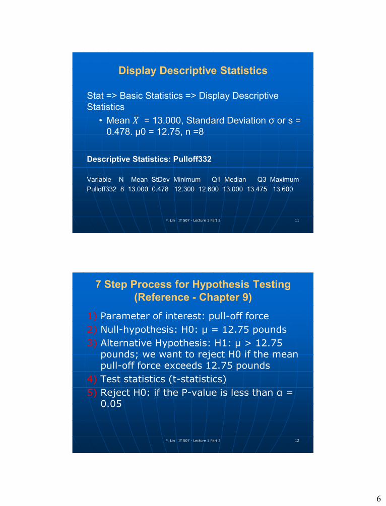
Display Descriptive Statistics
Stat => Basic Statistics => Display Descriptive
Statistics
• Mean 𝑋 = 13.000, Standard Deviation σ or s =
0.478. µ0 = 12.75, n =8
Descriptive Statistics: Pulloff332
Variable N Mean StDev Minimum Q1 Median Q3 Maximum
Pulloff332 8 13.000 0.478 12.300 12.600 13.000 13.475 13.600
P. Lin IT 507 - Lecture 1 Part 2 12
7 Step Process for Hypothesis Testing
(Reference - Chapter 9)
1) Parameter of interest: pull-off force
2) Null-hypothesis: H0: µ = 12.75 pounds
3) Alternative Hypothesis: H1: µ > 12.75 pounds; we want to reject H0 if the mean pull-off force exceeds 12.75 pounds
4) Test statistics (t-statistics)
5) Reject H0: if the P-value is less than α = 0.05
7
P. Lin IT 507 - Lecture 1 Part 2 13
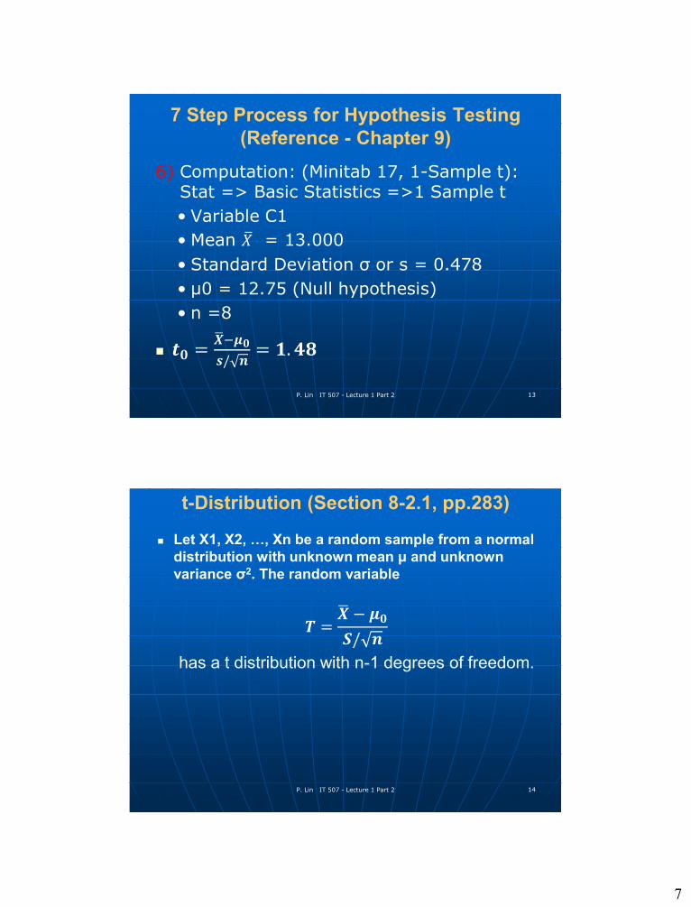
7 Step Process for Hypothesis Testing
(Reference - Chapter 9)
6) Computation: (Minitab 17, 1-Sample t): Stat => Basic Statistics =>1 Sample t
• Variable C1
• Mean 𝑋 = 13.000
• Standard Deviation σ or s = 0.478
• µ0 = 12.75 (Null hypothesis)
• n =8
𝒕𝟎 = 𝑿−𝝁𝟎
𝒔/ 𝒏= 𝟏. 𝟒𝟖
P. Lin IT 507 - Lecture 1 Part 2 14
t-Distribution (Section 8-2.1, pp.283)
Let X1, X2, …, Xn be a random sample from a normal
distribution with unknown mean μ and unknown
variance σ2. The random variable
𝑻 = 𝑿 − 𝝁𝟎
𝑺/ 𝒏
has a t distribution with n-1 degrees of freedom.

8
P. Lin IT 507 - Lecture 1 Part 2 15
Minitab 17 – 1-Sample tMinitab 17, 1-Sample t
StatGuide – One-Sample t (Summary)
The one-sample t-confidence interval and test
procedures are used to make inferences about a
population mean (μ ), based on data from a random
sample.
Suppose you have a sample of hole sizes from a drill
press and you want to determine if the machine is
drilling the correct size hole. Or, you may have a
sample of pizza delivery times and wish to
determine if you are beating your competitors
advertised delivery time of 30 minutes.
P. Lin IT 507 - Lecture 1 Part 2 16
Minitab 17 – 1-Sample tMinitab 17, 1-Sample t
StatGuide – One-Sample t (Summary)
Use one-sample t-procedures when you do not know
the standard deviation of the population (σ ). If you
know s, you can use the one-sample z-confidence
interval and test procedures instead.
To use the one-sample t-procedures, your sample
should also be normally distributed . If your sample
data do not appear to be normally distributed, you
should consider using an appropriate nonparametric
procedure .

9
P. Lin IT 507 - Lecture 1 Part 2 17
7 Step Process for Hypothesis Testing
(Reference - Chapter 9)
6) Computation: (Minitab 17, 1-
Sample t) Stat => Basic Statistics => 1 Sample t
Enter C1 into the Sample in Column dialog
box
CHECK the Perform hypothesis test and
enter 12.75 as Hypothesized mean, then
click OK
One-Sample T: Pulloff332
Test of mu = 12.75 vs > 12.75
95% Lower
Variable N Mean StDev SE Mean Bound T P
Pulloff332 8 13.000 0.478 0.169 12.680 1.48 0.091
P. Lin IT 507 - Lecture 1 Part 2 18
7 Step Process for Hypothesis Testing
6) Testing the Assumption of
Normality (Minitab 17) Stat => Basic Statistics => Normality
Test
Enter the following setting, as shown,
then click OK
14.013.513.012.512.0
99
95
90
80
70
60
50
40
30
20
10
5
1
Pulloff332
Pe
rce
nt
Mean 13
StDev 0.4781
N 8
AD 0.268
P-Value 0.576
Probability Plot of Pulloff332Normal

10
P. Lin IT 507 - Lecture 1 Part 2 19
7 Step Process for Hypothesis Testing
7) Conclusion (Ref. page 332-334, Book 1)
From Appendix A Table V (page 745, for a t-distribution
with 7 degrees of freedom (n -1=8-1), that t0 = 1.48 falls
between two values, 1.415 for which α = 0.1, and 1.895,
for which α = 0.05.
Because this is a one-tailed test, we know that the
Probability value or P-value is between those two values,
that is, 0.05 < P < 0.1.
Since P = 0.091 > 0.05, we do not have sufficient
evidence to reject H0 and conclude that the mean pull-
off force does not exceed 12.75 pounds
P. Lin IT 507 - Lecture 1 Part 2 20
Minitab – Glossary (Alpha α)
Used in hypothesis testing, alpha (a ) is the
maximum acceptable level of risk for rejecting a true
null hypothesis (type I error) and is expressed as a
probability ranging between 0 and 1. Alpha is
frequently referred to as the level of significance.
You should set a before beginning the analysis then
compare p-values to a to determine significance:
· If your p-value is less than or equal to the a-level,
reject the null hypothesis in favor of the alternative
hypothesis.
· If your p-value is greater than the a-level, fail to
reject the null hypothesis.
11
P. Lin IT 507 - Lecture 1 Part 2 21
Minitab – Glossary (Alpha α)
The most commonly used a-level is 0.05. At this
level, your chance of finding an effect that does not
really exist is only 5%. The smaller the a value, the
less likely you are to incorrectly reject the null
hypothesis. However, a smaller value for a also
means a decreased chance of detecting an effect if
one truly exists (lower power).
P. Lin IT 507 - Lecture 1 Part 2 22
Minitab – Glossary (p-value)
Determines the appropriateness of rejecting the null
hypothesis in a hypothesis test. P-values range
from 0 to 1. The p-value is the probability of
obtaining a test statistic that is at least as extreme
as the calculated value if the null hypothesis is true.
Before conducting any analyses, determine your
alpha (a) level. A commonly used value is 0.05. If the
p-value of a test statistic is less than your alpha, you
reject the null hypothesis.
12
P. Lin IT 507 - Lecture 1 Part 2 23
Minitab – Glossary (p-value)
Because of their fundamental role in hypothesis
testing, p-values are used in many areas of statistics
including basic statistics, linear models, reliability,
and multivariate analysis among many others. The
key is to understand what the null and alternative
hypotheses represent in each test and then use the
p-value to aid in your decision to reject the null.