iterative solvers for the maxwell–stefan diffusion ... · we consider a simplified...

Geiser, Cogent Mathematics (2015), 2: 1092913http://dx.doi.org/10.1080/23311835.2015.1092913

APPLIED & INTERDISCIPLINARY MATHEMATICS | RESEARCH ARTICLE

Iterative solvers for the Maxwell–Stefan diffusion equations: Methods and applications in plasma and particle transportJürgen Geiser1*

Abstract: In this paper, we are motivated to discuss a model based on a local ther-modynamic equilibrium, weakly ionized plasma-mixture model used for medical and technical applications in etching processes. For studying the model, we consider a simplified model based on the Maxwell–Stefan model, which describes multicompo-nent diffusive fluxes in the gas mixture. The MS model is more adequate to describe complex mixtures without dominating background species. Based on additional condi-tions to the fluxes, we obtain an irreducible and quasi-positive diffusion matrix. Such problems result in nonlinear diffusion equations, which are more delicate to solve as simpler standard diffusion equations with Fickian’s approach. Here, we propose an ef-ficient explicit time-discretization method, which is embedded to a fast iterative solver for the nonlinearities. Such a combination of coupling discretization and solver meth-ods allows to simulate the delicate nonlinear differential equations more effectively. We present the efficiency and accuracy of the iterative solvers for some first ternary component gaseous mixtures and discuss the details of the numerical methods.

Subject: Applied Mathematics; Mathematics Statistics; Science

Keywords: Maxwell–Stefan approach; plasma model; multicomponent mixture; explicit discretization schemes; iterative schemes

AMS subject classifications: 35K25; 35K20; 74S10; 70G65

*Corresponding author: Jürgen Geiser, The Institute of Theoretical Electrical Engineering, Ruhr University of Bochum, Universitätsstrasse 150, D-44801 Bochum, GermanyE-mail: [email protected]

Reviewing editor:Yong Hong Wu, Curtin University of Technology, Australia

Additional information is available at the end of the article

ABOUT THE AUTHORJürgen Geiser (http://homepage.ruhr-uni-bochum.de/Juergen.Geiser/), researcher and lecturer at the Ruhr-University of Bochum, Germany, has been involved in teaching and research projects and has collaborated with engineering and physicist groups on numerical modeling of technical and physical models. The research activity refers to the mathematical modeling, numerics, and analysis of transport and flow problems in engineering applications, e.g. groundwater modeling and plasma modelling. He is a specialist in multiscale solvers and iterative solvers and most of the topics of the special issue. Moreover, Juergen Geiser is the author of scientific books and editor of various scientific journals, and thus able to manage the editorial activity.

PUBLIC INTEREST STATEMENTA multicomponent model based on the Stefan–Maxwell approach is presented. Iterative solver approaches are used to solve the nonlinear modelling problem.

Received: 04 March 2015Accepted: 06 September 2015Published: 07 October 2015

© 2015 The Author(s). This open access article is distributed under a Creative Commons Attribution (CC-BY) 4.0 license.

of 16

http://crossmark.crossref.org/dialog/?doi=10.1080/23311835.2015.1092913&domain=pdf&date_stamp=2015-10-07

mailto:[email protected]


http://homepage.ruhr-uni-bochum.de/Juergen.Geiser/

http://homepage.ruhr-uni-bochum.de/Juergen.Geiser/

http://creativecommons.org/licenses/by/4.0/

of 16


1. IntroductionWe are motivated to understand the gaseous mixtures of a normal pressure and room temperature plasma. The understanding of normal pressure and room temperature plasma applications is impor-tant for applications in medical and technical processes. Since many years, the increasing impor-tance of plasma chemistry based on the multicomponent plasma is a key factor in understanding the gaseous mixture processes (see for low pressure plasma Senega & Brinkmann, 2006 and for atmospheric pressure regimes Tanaka, 2004).

We consider a simplified Maxwell–Stefan diffusion (MSD) equation to model the gaseous mixture of multicomponent plasma. Here, we consider of a macroscopic model, while the limits to apply to a kinetic (microscopic) model are discussed in Boudin, Grec, and Salvarani (2015). While the most clas-sical description of the diffusion goes back to the Fickian’s approach (see Fick, 1995), we apply the modern description of the multicomponent diffusion based on the Maxwell–Stefan’s approach (see Maxwell, 1867). The novel approach considers a more detailed description of the flux and concentra-tion, which are indeed not only proportionally coupled as in the simplified Fickian’s approach. Here, we deal with an inter-species force balance, which allows to model cross-effects, e.g. the so-called reverse diffusion (uphill diffusion in the direction of the gradients).

Such a more detailed modeling results in irreducible and quasi-positive diffusion matrices, which can be reduced by transforming with reductions or with Perron–Frobenius theorems to the solvable partial differential equations (see Bothe, 2011). The obtained system of nonlinear partial differential equations is delicate to solve with standard discretization and solver methods. Therefore, we have taken into account effective linearization methods, e.g. iterative fix-point schemes, to overcome the nonlinearities. Alternative methods exist and are explained in Böttcher (2010) and Spille-Kohoff, Preuß, and Böttcher (2012). Here, they reduce the MSD equation and solve it explicitly, but such methods are restricted to ternary or quaternary systems. Further multicomponent approaches with MSD equations are discussed for only stationary problems, while the solver methods embed the nonlinear MSD approaches into the finite volume discretization schemes (see Peerenboom, van Boxtel, Janssen, & van Dijk, 2014). Such approximations lack with respect to solve nonstationary problems.

The paper is outlined as follows.

In Section 2, we present our mathematical model. A possible reduced model for the further approximations is derived in Section 3. In Section 4, we discuss the underlying numerical schemes. The first numerical results are presented in Section 5. In the contents, that are given in Section 6, we summarize our results.

2. Mathematical modelFor the full plasma model, we assume that the neutral particles can be described as the fluid dynamical model, where the elastic collision defines the dynamics and few inelastic collisions are, among other reasons, responsible for the chemical reactions.

To describe the individual mass densities, as well as the global momentum and the global energy as the dynamical conservation quantities of the system, corresponding conservation equations are derived from Boltzmann equations.

The individual character of each species is considered by mass conservation equations and the so-called difference equations.

The extension of the nonmixtured multicomponent transport model (Senega & Brinkmann, 2006) is done with respect to the collision integrals related to the right-hind side sources of the conserva-tion laws.

of 16


The conservation laws of the neutral elements are given as

where �s : density of species i, � =∑N

i=1 �i, u : velocity, and ∗

tot : total energy of the neutral particles.

Further, the variable Q(s)n is the collision term of the mass conservation equation, Q(e)

m is the collision term of the momentum conservation equation, and Q(e)

is the collision term of the energy conserva-tion equation.

We derive the collision term with respect to the Chapmen–Enskog method (see Chapman & Cowling, 1990) and achieve for the first derivatives the following results:

where i = 1,… ,ns, Fi is an external force per unit mass (see Boltzmann equation); further, the diffu-sion velocity is given as:

where ∑N

i=1 di = 0,

where xi =ns

n is the molar fraction of species i.

We have an additional constraint based on the mass fraction of each species:

where yi is the mass fraction of species i and Ri is the net production rate of species i due to the reactions.

�

�t�s +

�

�r⋅ �sus = msQ

(s)n ,

�

�t�u +

�

�r⋅

(P∗ + �uu

)= −Q(e)

m ,

�

�t∗

tot +�

�r⋅

(∗

totu + q∗ + P∗ ⋅ u

)= −Q(e)

,

(1)msQ

(s)n = −∇ ⋅ (�i

∑j=0

�j

i),

(2)Q(e)m = −

ns∑i=1

�iFi ,

(3)Q(e)

= −

ns∑i=1

�i�Fi(� +∑j=0

V(j)

i),

(4)�0

i = 0,

(5)�1

i = −

N∑j=1

Dij(dj + kTjΔT

T),

(6)di = ∇xi + xi∇p

p−

�i

�Fi ,

(7)di = di − yi

∑j

d∗

j ,

(8)�

�tyi + ∇yi = Ri(y1,… , yN),

of 16


Remark 1 The full model problem considers a fully coupled system of conservation laws and Maxwell–Stefan equations. Each equation is coupled such that the gaseous mixture influences the transport equations and vice versa. In the following, we decouple the equations system and con-sider only the delicate Maxwell–Stefan equations.

3. Simplified model with Maxwell–Stefan diffusion equationsWe discuss in the following a multicomponent gaseous mixture with three species (ternary mixture). The model problem is discussed in the experiments of Duncan and Toor (1962).

Here, they studied an ideal gaseous mixture of the following components:

(1) Hydrogen (H2, first species),

(2) Nitrogen (N2, second species), and

(3) Carbon dioxide (CO2, third species).

The Maxwell–Stefan equations are given for the three species as (see also Boudin, Grec, & Salvarani, 2012):

where the domain is given as Ω ∈ IRd,d ∈ IN+ with �i ∈ C

2.

For such ternary mixture, we can rewrite the three differential Equations (9) and (11 and 12) with the help of the zero-condition (10) into two differential equations, given as:

where � =(

1

D12

−1

D13

) and � =

(1

D12

−1

D23

).

Further, we have the relations:

(1) Third mole fraction: �3= 1 − �

1− �

2,

(2) Third molar flux: N3= −N

1− N

2.

(9)�t�i + ∇ ⋅ Ni = 0, 1 ≤ i ≤ 3,

(10)3∑j=1

Nj = 0,

(11)�2N1− �

1N2

D12

+�3N1− �

1N3

D13

= −∇�1,

(12)�1N2− �

2N1

D12

+�3N2− �

2N3

D23

= −∇�2,

(13)�t�i + ∇ ⋅ Ni = 0, 1 ≤ i ≤ 2,

(14)1

D13

N1+ �N

1�2− �N

2�1= −∇�

1,

(15)1

D23

N2− �N

1�2+ �N

2�1= −∇�

2,

of 16


4. Numerical methodsIn the following, we discuss the numerical methods which are based on iterative schemes with embedded explicit discretization schemes (see also Geiser, 2015, in press). We apply the following methods:

(1) Iterative scheme in time (global linearization with matrix method),

(2) Iterative scheme in time (local linearization with Richardson’s method).

For spatial discretization, we apply finite volume or finite difference methods. The underlying time discretization is based on a first-order explicit Euler method.

4.1. Iterative scheme in time (global linearization with matrix method)We solve the iterative scheme:

for j = 0,… , J , where �n1= (�n

1,0,… , �n

1,J)T, �

n2= (�n

2,0,… , �n

2,J)T and IJ ∈ IR

J+1× IR

J+1, Nn1= (Nn

1,0,… ,Nn

1,J)T, Nn

2= (Nn

2,0,… ,Nn

2,J)T and IJ ∈ IR

J+1× IR

J+1, where n = 0, 1, 2,… ,Nend and Nend are the number of time steps, i.d. Nend = T∕Δt.

The matrices are given as:

meaning that the diagonal entries given for the scale case in Equation (13) and the outer diagonal entries are zero.

The explicit form with time discretization is given as:

(16)�n+11

= �n1− Δt D

+Nn1,

(17)�n+12

= �n2− Δt D

+Nn2,

(18)(A B

C D

)(Nn+11

Nn+12

)=

(−D

−�n+11

−D−�n+12

),

(19)A,B,C,D ∈ IRJ+1

× IRJ+1,

(20)Aj, j =1

D13

+ ��2,j , j = 0… , J,

(21)Bj, j = −��1, j , j = 0… , J,

(22)Cj, j = −��2,j , j = 0… , J,

(23)Dj, j =1

D23

+ ��1,j , j = 0… , J,

(24)Ai, j = Bi,j = Ci,j = Di,j = 0, i, j = 0… , J, i ≠ J,

of 16


of 16


4.2. Iterative scheme in time (local linearization with Richardson’s methodWe solve the iterative scheme given in the Richardson iterative scheme:

for j = 0,… , J , where �n1= (�n

1,0,… , �n

1,J)T, �

n2= (�n

2,0,… , �n

2,J)T and IJ ∈ IR

J+1× IR

J+1, Nn1= (Nn

1,0,… ,Nn

1,J)T, Nn

2= (Nn

2,0,… ,Nn

2,J)T and IJ ∈ IR

J+1× IR

J+1, where n = 0, 1, 2,… ,Nend and Nend are the number of time steps, i.d. Nend = T∕Δt.

Further, k = 1, 2,… ,K is the iteration index where �n+1,01

= (�n1,0,… , �n

1,J)T, �n+1,0

2= (�n

2,0,… , �n

2,J)T,

and IJ ∈ IRJ+1

× IRJ+1 is the start solution given with the solution at t = tn.

The matrices are given as:

(47)�n+1,k

1= �

n1− Δt D

+Nn+11,

(48)�n+1,k

2= �

n2− Δt D

+Nn+12,

(49)(An+1,k−1 Bn+1,k−1

Cn+1,k−1 Dn+1,k−1

)(Nn+11

Nn+12

)=

(−D

−�n+1,k−1

1

−D−�n+1,k−1

2

),

(50)An+1,k−1,Bn+1,k−1,Cn+1,k−1,Dn+1,k−1 ∈ IRJ+1 × IRJ+1,

(51)An+1,k−1j,j

=1

D13

+ ��n+1,k−1

2,j, j = 0… , J,

(52)Bn+1,k−1j,j

= −��n+1,k−1

1,j, j = 0… , J,

(53)Cn+1,k−1j,j

= −��n+1,k−1

2,j, j = 0… , J,

(54)Dn+1,k−1j,j

=1

D23

+ ��n+1,k−1

1,j, j = 0… , J,

(55)An+1,i−1i,j

= Bn+1,i−1i,j

= Cn+1,i−1i,j

= Dn+1,i−1i,j

= 0, i, j = 0… , J, i ≠ J,

of 16


meaning that the diagonal entries given for the scale case in Equation (95) and the outer diagonal entries are zero.

The explicit form with time discretization is given as:

of 16


5. Numerical experimentsIn the following, we concentrate on the following three-component system, which is given as:

where the domain is given as Ω ∈ IRd,d ∈ IN+ with �i ∈ C

2.

The parameters and the initial and boundary conditions are given as:

(1) D12

= D13

= 0.833 (means � = 0) and D23

= 0.168 (Uphill diffusion, semi-degenerated Duncan and Toor experiment),

(78)�t�i + �xNi = 0, 1 ≤ i ≤ 3,

(79)3∑j=1

Nj = 0,

(80)�2N1− �

1N2

D12

+�3N1− �

1N3

D13

= −�x�1,

(81)�1N2− �

2N1

D12

+�3N2− �

2N3

D23

= −�x�2,

of 16


(2) D12

= 0.0833,D13

= 0.680 and D23

= 0.168 (asymptotic behavior, Duncan and Toor experi-ment (see Duncan & Toor, 1962)),

(3) J = 140 (spatial grid points),

(4) The time step restriction for the explicit method is given as: Δt ≤ (Δx)2

2max{D12,D13,D23},

(5) The spatial domain is Ω = [0, 1], the time-domain [0, T] = [0, 1],

(6) The initial conditions are:

(i) Uphill example

(ii) Diffusion example (Asymptotic behavior)

(7) The boundary conditions are of no-flux type:

We could reduce to a simpler model problem as:

where � =(

1

D12

−1

D13

), � =

(1

D12

−1

D23

).

We rewrite into:

and we have

(82)𝜉in1(x) =

⎧⎪⎨⎪⎩

0.8 if 0 ≤ x < 0.25,

1.6(0.75 − x) if 0.25 ≤ x < 0.75,

0.0 if 0.75 ≤ x ≤ 1.0,

(83)�in2(x) = 0.2, for all x ∈ Ω = [0, 1].

(84)�in1(x) =

{0.8 if 0 ≤ x ∈ 0.5,

0.0 else,

(85)�in2(x) = 0.2, for all x ∈ Ω = [0, 1].

(86)N1= N

2= N

3= 0, on �Ω × [0, 1].

(87)�t�i + �x ⋅ Ni = 0, 1 ≤ i ≤ 2,

(88)1

D13

N1+ �N

1�2− �N

2�1= −�x�1,

(89)1

D23

N2− �N

1�2+ �N

2�1= −�x�2,

(90)�t�1 + �x ⋅ N1 = 0,

(91)�t�2 + �x ⋅ N2 = 0,

(92)

( 1

D13

+ ��2

−��1

−��2

1

D23

+ ��1

)(N1

N2

)=

(−�x�1−�x�2

),

(93)�t�1 + �x ⋅ N1 = 0,

of 16


The next step is to apply the semi-discretization of the partial differential operator ��x

.

We apply the first differential operator in Equations (93) and (94) as an forward upwind scheme given as

and the second differential operator in Equation (95) as an backward upwind scheme given as

5.1. Experiments with the iterative scheme in time (global linearization)In the first experiments, we test the first iterative scheme (iterative scheme in time (global linearization)).

We test the different experiments (uphill and diffusion examples) and obtain the results as shown in Figure 1 for the uphill example.

Remark 2 In Figure 1, we obtain a typical complex mixture, without dominating background gas. While the concentration �

1 increases and �

3 decreases, the important concentration �

2 decreases and

increases around the value 0.2. Such a behavior cannot be produced with simple standard Fickian’s approach and here it is important to deal with the MS approach.

The concentration and their fluxes are given in Figure 2.

(94)�t�2 + �x ⋅ N2 = 0,

(95)(N1

N2

)=

D13D23

1 + �D13�2+ �D

23�1

( 1

D23

+ ��1

��1

��2

1

D13

+ ��2

)(−�x�1−�x�2

).

(96)�

�x= D

+=

1

Δx⋅

⎛⎜⎜⎜⎜⎜⎝

−1 0 … 0

1 −1 0 … 0

⋮ ⋱ ⋱ ⋱ ⋮

0 1 −1 0

0 … 0 1 −1

⎞⎟⎟⎟⎟⎟⎠

∈ IR(J+1)×(J+1)

,

(97)�

�x= D

−=

1

Δx⋅

⎛⎜⎜⎜⎜⎜⎝

−1 1 0 … 0

0 −1 1 0 …

⋮ ⋱ ⋱ ⋱ ⋱

0 … 0 −1 1

0 … 0 −1

⎞⎟⎟⎟⎟⎟⎠

∈ IR(J+1)×(J+1)

.

Figure 1. Results of the mole fraction (concentration) �

1, �

2

and �3.

0 0.2 0.4 0.6 0.8 10

0.1

0.2

0.3

0.4

0.5

0.6

0.7

0.8

t

x=0.72

1

2

3

of 16


Remark 3 In Figure 2, we obtain a fine resolved behavior of the important second species �2. Here,

we see detailed the oscillatory behavior of the flux N2 and the concentration gradient −�x�2 in the

time interval t = [0, 1]. For the next time interval t = [1, 2], we obtained a stabilized behavior of the complex mixture. Here, it is important to resolve the nonlinearity very accurately for unstable initiali-zation of the complex mixture.

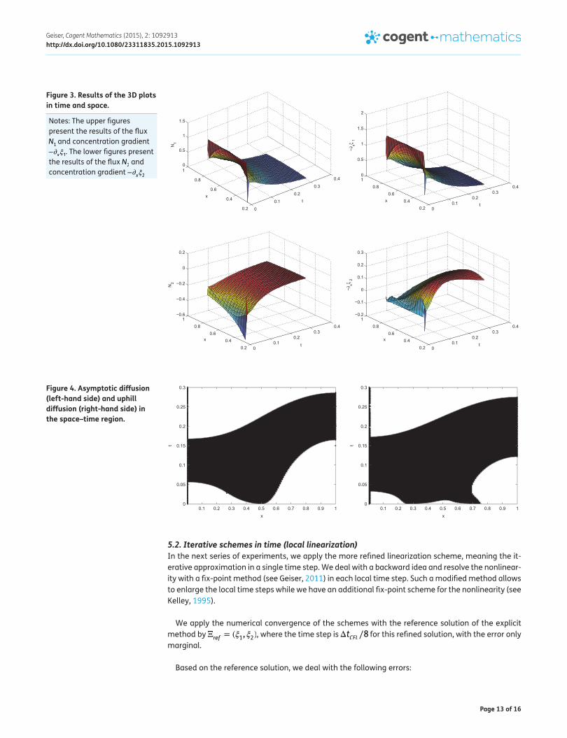
The full plots in time and space of the concentrations and their fluxes are given in Figure 3.

The space–time regions where −N2�x�2 ≥ 0 for the uphill diffusion and asymptotic diffusion, giv-en in Figure 4.

Remark 4 In Figure 3, we present the delicate unstable behavior of the mixture around time scale t = [0, 1] and the spatial scale x = [0, 1] in a 3D plot with the first and second concentration. The steep gradients of the concentrations have to be resolved with a very fine time step. We also obtain the same delicate results of the initialization process in Figure 4. Here, we present the space–time regions for the uphill and asymptotic diffusions. In both experiments, we see that we have a back-flow of the mixture, meaning the second concentration �

2 has both decreasing and increasing gradi-

ents. For both experiments, we resolve the initial process with fine time steps.

Remark 5 In the first numerical method, we apply global linearization based on the time steps. Meaning, we deal with an explicit time discretization that solves the linearized equation forward. All effects are resolved by taking into account the CFL condition. Therefore, we achieve better results with finer time steps, e.g. ΔtCFl∕8, such that the global linearization, via the time step, is important for our first numerical method.

Figure 2. Concentration and flux of iterative scheme in time (global linearization).

0 0.2 0.4 0.6 0.8 10

0.2

0.4

0.6

0.8

1

1.2

1.4

t

N1

x=0.72

0 0.2 0.4 0.6 0.8 10

0.2

0.4

0.6

0.8

1

1.2

1.4

1.6

t

−x

1

x=0.72

0 0.2 0.4 0.6 0.8 1−0.25

−0.2

−0.15

−0.1

−0.05

0

0.05

0.1

t

N2

x=0.72

0 0.2 0.4 0.6 0.8 1−0.02

0

0.02

0.04

0.06

0.08

0.1

0.12

t

−x

2

x=0.72

Notes: The upper figures present the results of the flux N1 and concentration gradient

−�x�1. The lower figures present the results of flux N

2 and

concentration gradient −�x�2.

of 16


5.2. Iterative schemes in time (local linearization)In the next series of experiments, we apply the more refined linearization scheme, meaning the it-erative approximation in a single time step. We deal with a backward idea and resolve the nonlinear-ity with a fix-point method (see Geiser, 2011) in each local time step. Such a modified method allows to enlarge the local time steps while we have an additional fix-point scheme for the nonlinearity (see Kelley, 1995).

We apply the numerical convergence of the schemes with the reference solution of the explicit method by Ξref = (�

1, �2), where the time step is ΔtCFL∕8 for this refined solution, with the error only

marginal.

Based on the reference solution, we deal with the following errors:

Figure 3. Results of the 3D plots in time and space.

0

0.1

0.2

0.3

0.4

0.2

0.4

0.6

0.8

10

0.5

1

1.5

tx

N1

00.1

0.20.3

0.4

0.20.4

0.60.8

10

0.5

1

1.5

2

tx

−x

10

0.10.2

0.30.4

0.20.4

0.60.8

1−0.6

−0.4

−0.2

0

0.2

tx

N2

00.1

0.20.3

0.4

0.20.4

0.60.8

1−0.2

−0.1

0

0.1

0.2

0.3

tx

−x

2

Figure 4. Asymptotic diffusion (left-hand side) and uphill diffusion (right-hand side) in the space–time region.

x

t

0.1 0.2 0.3 0.4 0.5 0.6 0.7 0.8 0.9 10

0.05

0.1

0.15

0.2

0.25

0.3

x

t

0.1 0.2 0.3 0.4 0.5 0.6 0.7 0.8 0.9 10

0.05

0.1

0.15

0.2

0.25

0.3

Notes: The upper figures present the results of the flux N1 and concentration gradient

−�x�1. The lower figures present the results of the flux N

2 and

concentration gradient −�x�2

of 16


where method, J is the Richardson method (second method, see Section 4.1) with J iterative steps and Δt = ΔtCFL,ΔtCFL∕2,ΔtCFL∕4.

Further, method, expl is the explicit method (first method, see Section 4.2) with Δt = ΔtCFL,ΔtCFL∕2,ΔtCFL∕4.

We apply different versions of time steps and iterative steps and a reference solution is obtained with a fine time step Δt = ΔtCFL∕4. We see improvements in Figure 5 and the errors in Figure 6.

Remark 6 In Figure 5, we compare a reference solution (first method) with fine time steps with flex-ible time step and iterative step solutions (second method). We obtain some accurate solutions with the second method with more larger time steps and more iterative steps. Based on the large time steps, the computational time decreases and additional number of more iterative cycles did not in-fluence the amount of computational work.

Remark 7 In Figure 6, we present the L1 errors of the second method (local linearization) compared

with the reference solution (first method with very fine time steps). Here, we see the benefit of large time steps with N = 100 and K = 800, meaning we have only 100 time steps and 800 iterative steps, which are not expensive. Therefore, we could gain the same results as with many small time steps N = 80000 and only one iterative step K = 1, such that the relaxation method benefits with the itera-tive cycles and we could enlarge the time steps. We obtain the same accurate results for larger time

(98)EL

1,Δx(t) = ∫

Ω

|Ξmethod,J,Δx(x, t) − Ξref (x, t)| dx

= Δx

N∑i=1

|Ξmethod,J,Δx(xi , t) − Ξref (xi , t)|,

Figure 6. Errors of the different time step and iterative step solutions of the second method (left-hand side: error with the reference solution at the full time interval t ∈ [0, 1.4] and right-hand side: error with the reference solutions at the initial time interval t ∈ [0, 0.1]).

0 0.2 0.4 0.6 0.8 1 1.2 1.40

0.002

0.004

0.006

0.008

0.01

0.012

t

Err L1

x=0.72

N=80000 K=1N=10000 K=8N=1000 K=80N=100 K=800

0 0.02 0.04 0.06 0.08 0.10

0.002

0.004

0.006

0.008

0.01

0.012

t

Err L1

x=0.72

N=80000 K=1N=10000 K=8N=1000 K=80N=100 K=800

Figure 5. Solutions of different time steps and iterative steps of the Richardson method (left-hand side: concentration �

1 and

right-hand side: concentration �2).

0 0.2 0.4 0.6 0.8 1 1.2 1.40

0.05

0.1

0.15

0.2

0.25

0.3

0.35

0.4

t

1

x=0.72

cfl/4N=80000 K=1N=10000 K=8N=1000 K=80N=100 K=800

0 0.2 0.4 0.6 0.8 1 1.2 1.40.155

0.16

0.165

0.17

0.175

0.18

0.185

0.19

0.195

0.2

0.205

t

2

x=0.72

cfl/4N=80000 K=1N=10000 K=8N=1000 K=80N=100 K=800

of 16


steps, instead of a computational intensive fine resolution with small time steps. Such a novel treat-ment with a local linearization and additional iterative cycles reduces the computational amount of the novel second scheme.

Remark 8 The second method applies a linear linearization based on the iterative approaches in each single time step. The spatial and time discretizations are embedded into the iterative solver method. We have the benefit of relaxation in each local time step with the high resolution of the spatial and timescales. Therefore, we see a more accurate solution also with larger time steps than in the global linearization method.

6. Conclusions and discussionWe present a fluid model based on a delicate mixture of components. Such a model can be resolved by a MSD equation, while we can embed the complex mixture processes. The underlying problems for such a more delicate diffusion matrix are discussed. Based on a delicate nonlinear partial differential equation, which has to be reduced to a solvable linearized partial differential equation, we have to discuss two linearization approaches. The first approach deals with a global linearization, which can be controlled by the time steps. The second approach deals with a local linearization and applies an iterative scheme. Such a novel approach is more flexible and can be controlled by the time steps and additionally with the iterative steps. Therefore, we obtain the same accuracy with much more larger time steps and moderate iterative steps and reduce the computational amount. For the first test ex-amples, we achieve more accurate results for a new local linearized scheme and optimize their com-putational amount with larger time steps. In future, we concentrate on numerical convergence analysis of the local linearization schemes and generalize our results to real-life applications.

FundingThe author has received no direct funding for this research.

Author detailsJürgen Geiser1

E-mail: [email protected] ID: http://orcid.org/0000-0003-1093-00011 The Institute of Theoretical Electrical Engineering, Ruhr

University of Bochum, Universitätsstrasse 150, D-44801 Bochum, Germany.

Citation informationCite this article as: Iterative solvers for the Maxwell–Stefan diffusion equations: Methods and applications in plasma and particle transport, Jürgen Geiser, Cogent Mathematics (2015), 2: 1092913.

ReferencesBothe, D. (2011). On the Maxwell--Stefan approach to

multicomponent diffusion. Parabolic Problems, Progress in Nonlinear Differential Equations and Their Applications, 80, 81–93. doi:10.1007/978-3-0348-0075-4_5

Böttcher, K. (2010). Numerical solution of a multicomponent species transport problem combining diffusion and fluid flow as engineering benchmark. International Journal of Heat and Mass Transfer, 53, 231–240. doi:10.1016/j.ijheatmasstransfer.2009.09.038

Boudin, L., Grec, B., & Salvarani, F. (2012). A mathematical and numerical analysis of the Maxwell-Stefan diffusion equations. Discrete and Continuous Dynamical Systems Series B, 17, 1427–1440.

Boudin, L., Grec, B., & Salvarani, F. (2015). The Maxwell--Stefan diffusion limit for a kinetic model of mixtures. Acta Applicandae Mathematicae, 136, 79–90. doi:10.1007/s10440-014-9886-z

Chapman, S., & Cowling, Th. G. (1990). The mathematical theory of non-uniform gases: An account of the kinetic theory of viscosity, thermal conduction, and diffusion in gases. Cambridge: Cambridge University Press.

Duncan, J. B., & Toor, H. L. (1962). An experimental study of three component gas diffusion. AIChE Journal, 8, 38–41. doi:10.1002/aic.690080112

Fick, A. (1995). On liquid diffusion. Journal of Membrane Science, 100, 33–38. doi:10.1016/0376-7388(94)00230-V

Geiser, J. (2011). Iterative splitting methods for differential equations. Boca Raton, FL: CRC-Press.

Geiser, J. (2015). Numerical methods of the Maxwell--Stefan diffusion equations and applications in plasma and particle transport. arxiv:1501.05792. Retrieved from http://arxiv.org/abs/1501.05792

Geiser, J. (in press). Multicomponent and multiscale systems: Theory, methods, and applications in engineering. New York, NY: Springer International.

Kelley, C. T. (1995). Iterative methods for linear and nonlinear equations. Philadelphia, PA: SIAM.

Maxwell, J. C. (1867). On the dynamical theory of gases. Philosophical Transactions of the Royal Society, 157, 49–88. Retrieved from http://www.jstor.org/stable/108968?seq=1#page_scan_tab_contents

Peerenboom, K., van Boxtel, J., Janssen, J., & van Dijk, J. (2014). A conservative multicomponent diffusion algorithm for ambipolar plasma flows in local thermodynamic equilibrium. Journal of Physics D: Applied Physics, 47, 425202. doi:10.1088/0022-3727/47/42/425202

Senega, T. K., & Brinkmann, R. P. (2006). A multi-component transport model for non-equilibrium low-temperature low-pressure plasmas. Journal of Physics D: Applied Physics, 39, 1606–1618. doi:10.1088/0022-3727/39/8/020

Spille-Kohoff, A., Preuß, E., & Böttcher, K. (2012). Numerical solution of multi-component species transport in gases at any total number of components. International Journal of Heat and Mass Transfer, 55, 5373–5377. doi:10.1016/j.ijheatmasstransfer.2012.05.040

Tanaka, Y. (2004). Two-temperature chemically non-equilibrium modelling of high-power Ar-N2 inductively coupled plasmas at atmospheric pressure. Journal of Physics D: Applied Physics, 37, 1190–1205. doi:10.1088/0022-3727/37/8/007


http://orcid.org/0000-0003-1093-0001

http://dx.doi.org/10.1007/978-3-0348-0075-4_5

http://dx.doi.org/10.1016/j.ijheatmasstransfer.2009.09.038


http://dx.doi.org/10.1007/s10440-014-9886-z

http://dx.doi.org/10.1007/s10440-014-9886-z

http://dx.doi.org/10.1002/aic.690080112

http://dx.doi.org/10.1016/0376-7388(94)00230-V

http://arxiv.org/abs/1501.05792

http://www.jstor.org/stable/108968?seq=1#page_scan_tab_contents

http://www.jstor.org/stable/108968?seq=1#page_scan_tab_contents

http://dx.doi.org/10.1088/0022-3727/47/42/425202

http://dx.doi.org/10.1088/0022-3727/39/8/020



http://dx.doi.org/10.1088/0022-3727/37/8/007

of 16


© 2015 The Author(s). This open access article is distributed under a Creative Commons Attribution (CC-BY) 4.0 license.You are free to: Share — copy and redistribute the material in any medium or format Adapt — remix, transform, and build upon the material for any purpose, even commercially.The licensor cannot revoke these freedoms as long as you follow the license terms.

Under the following terms:Attribution — You must give appropriate credit, provide a link to the license, and indicate if changes were made. You may do so in any reasonable manner, but not in any way that suggests the licensor endorses you or your use. No additional restrictions You may not apply legal terms or technological measures that legally restrict others from doing anything the license permits.

Cogent Mathematics (ISSN: 2331-1835) is published by Cogent OA, part of Taylor & Francis Group. Publishing with Cogent OA ensures:• Immediate, universal access to your article on publication• High visibility and discoverability via the Cogent OA website as well as Taylor & Francis Online• Download and citation statistics for your article• Rapid online publication• Input from, and dialog with, expert editors and editorial boards• Retention of full copyright of your article• Guaranteed legacy preservation of your article• Discounts and waivers for authors in developing regionsSubmit your manuscript to a Cogent OA journal at www.CogentOA.com

iterative solvers for the maxwell–stefan diffusion ... · we consider a simplified...

Documents