the maxwell-stefan equations - james c. sutherland 12: drag coefﬁcient for drag that particle...

The Maxwell-Stefan Equations

ChEn 6603

1Friday, February 4, 2011

Outline

Diffusion in “ideal,” binary systems• Particle dynamics

• Maxwell-Stefan equations

• Fick’s Law

Diffusion in “ideal” multicomponent systems• Example: Stefan tube

• Matrix form of the Maxwell-Stefan equations

• Fick’s Law for multicomponent systems

• Reference velocities again


Particle DynamicsConservation of momentum:

m1(u1 − uf1) + m2(u2 − uf2) = 0

Conservation of kinetic energy (elastic collision):

m1(u21 − u2

f1) + m2(u22 − u2

f2) = 0

Solve for final particle velocities:

Sum of forces acting on particles of type “1” per unit volume

Rate of change of momentum of

particles of type “1” per unit volume

Momentum exchanged per

collision between “1” and “2”

Rate of 1-2 collisions per unit volume

×∝∝u1 − u2 x1x2

Momentum exchanged in a collision:m1(u1 − uf1) = m1u1 −

m1

m1 + m2(u1(m1 −m2) + 2m2u2) ,

=2m1m2(u1 − u2)

m1 + m2.

uf1 =u1(m1 −m2) + 2m2u2

m1 + m2,

uf2 =u2(m2 −m1) + 2m1u1

m1 + m2

u1

u2

m2

m1

T&K §2.1.1-2.1.2

For molecules, inelastic collisions are known by

another name ... what is it?


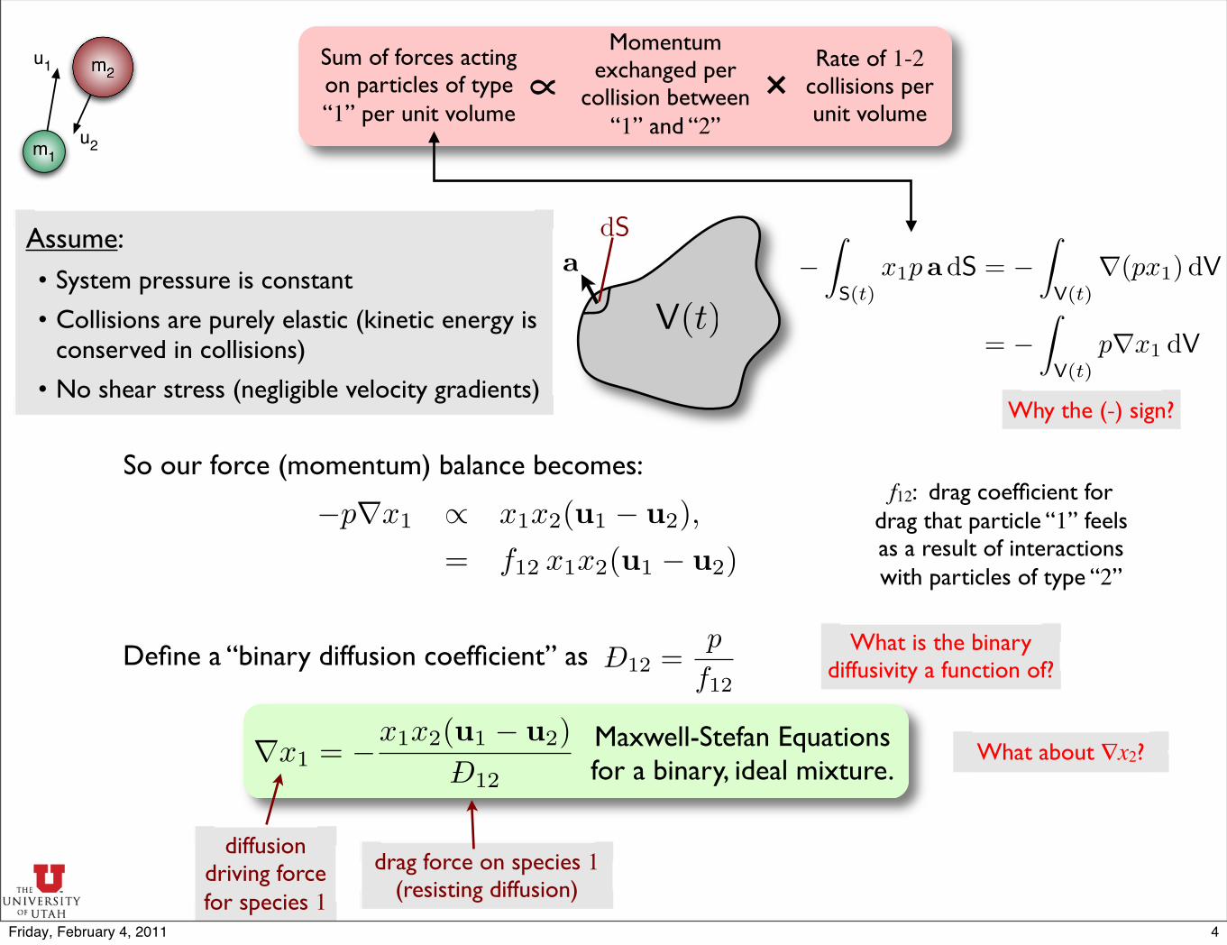
f12: drag coefficient for drag that particle “1” feels as a result of interactions with particles of type “2”

Maxwell-Stefan Equations for a binary, ideal mixture.

u1

u2

m2

m1

adS

V(t)

Assume:• System pressure is constant

• Collisions are purely elastic (kinetic energy is conserved in collisions)

• No shear stress (negligible velocity gradients)

So our force (momentum) balance becomes:

Define a “binary diffusion coefficient” as What is the binary diffusivity a function of?

What about ∇x2?

D12 =p

f12

∇x1 = −x1x2(u1 − u2)D12

Why the (-) sign?

−p∇x1 ∝ x1x2(u1 − u2),= f12 x1x2(u1 − u2)

Sum of forces acting on particles of type “1” per unit volume

Momentum exchanged per

collision between “1” and “2”

Rate of 1-2 collisions per unit volume

×∝

diffusion driving force for species 1

drag force on species 1 (resisting diffusion)

−�

S(t)x1pa dS = −

�

V(t)∇(px1) dV

= −�

V(t)p∇x1 dV


∇x1 = −x1x2(u1 − u2)D12

Fick’s Law - Binary Ideal System

Maxwell-Stefan equations for a binary, ideal system at constant pressure.

J1 = −ctD12∇x1

∇x1 = −x2N1 − x1N2

ctD12

= −x2J1 − x1J2

ctD12

∇x1 = − J1

ctD12

Fick’s law for a binary, ideal system at constant pressure

can you show this?


Re-Cap

Đ12 can be interpreted as an inverse drag coefficient. Đ12 = Đ21 (symmetric due to momentum conservation) Đ12 depends on the characteristics of species 1 and 2 (molecule shapes, etc.), but not on their relative compositions. Đ12 may depend on temperature and pressure.We call Đ12 the “Maxwell-Stefan” diffusivity or “Binary” diffusivity.

There are no “1-1” interactions here - Đ11 is not defined.


Multicomponent Systemsu1

u2

m2

m1

u3

m3

What about i=j?

Ternary system: must consider 1-2, 1-3, and 2-3 interactions.

Multicomponent system: must consider i-j interactions.

in general...

Ni = xicui Ji = Ni − xicuRecall:

di = ∇xi

(so far)

Assumptions:• Constant Pressure

• Ideal mixture (elastic collisions)‣ Conservation of translational energy.

‣ Where else could the energy go?

∇x1 = −x1x2(u1 − u2)D12

− x1x3(u1 − u3)D13

∇x1 = −x1x2(u1 − u2)D12

Binary system:

T&K §2.1.3-2.1.4

∇x2 = −x1x2(u2 − u1)D12

− x2x3(u2 − u3)D23

∇xi = −n�

j=1j �=i

xixj(ui − uj)

Ðijdi = −

n�

j=1j �=i

xixj(ui − uj)

Ðij

di = −n�

j �=i

xjNi − xiNj

cDij,

= −n�

j �=i

xjJi − xiJj

cDij


Example: Stefan Tube

∂cxi

∂t=

∂ci

∂t= −∇ · Ni

∂ρωi

∂t=

∂ρi

∂t= −∇ · ni,

At steady state (1D),

Species balance equations (no reaction):

T&K Example 2.1.1

Acetone (1), Methanol (2), Air (3)

Given: Đij, xi(z=0), xi(z=ℓ)

Find xi(z)

Air

LiquidMixture

z = �

z = 0

From the Maxwell-Stefan equations:

Convection-diffusion balance...

D12 = 8.48 mm2/sD13 = 13.72 mm2/sD23 = 19.91 mm2/s

x1(z=0)=0.319, x2(z=0)=0.528

ni = αi

Ni = βi

dxi

dz= −

n�

j �=i

xjNi − xiNj

ctÐij


1

�

dxi

dη=

n�

j=1j �=i

xiNj − xjNi

ctÐij,

= xi

n�

j �=i

Nj

ctÐij− xnNi

ctÐin−

n−1�

j �=i

xjNi

ctÐij

Eliminate xn by substituting:

We need to eliminate xn from the equation so that we have unknowns x1 ... xn-1.

xn = 1−n−1�

j=1

= 1− xi −n−1�

j �=i

xj

move l over.

Normalized coordinate:

η ≡ z

�,

d

dz=

d

dη

dη

dz=

1

�

d

dηMaxwell-Stefan

Equations

Split the first summation term and rearrange a bit, collecting terms on xi, xj.

A semi-analytic solution

almost there...

dxi

dz= −

n�

j �=i

xjNi − xiNj

ctÐij

1

�

dxi

dη= xi

n�

j �=i

Nj

ctÐij− Ni

ctÐin

1− xi −n−1�

j �=1

xj

−n−1�

j �=i

xjNi

ctÐij,

= xi

Ni

ctÐin+

n�

j �=i

Nj

ctÐij

− Ni

ctÐin+

n−1�

j �=i

�Ni

ctÐin− Ni

ctÐij

�xj ,

dxi

dη= =

Ni

ctÐin/�+

n�

j �=i

Nj

ctÐij/�

� �� Φii

xi +n−1�

j �=i

�Ni

ctÐin/�− Ni

ctÐij/�

�

� �� Φij

xj −Ni

ctÐin/�� φi


Analytic solution (assuming Ni are all constant)

see T&K §8.3 and Appendix B

Matrix exponential!exp[Φ] ≠ [exp(Φij)]!In Matlab, use “expm”

(x) =�exp [[Φ] η]

�(x0) +

�[exp [[Φ] η]]− [I]

��Φ�−1

(φ)

1. Guess Ni

2. Calculate [Φ], (φ)3. Calculate (x) at η=1 (z=l)

4. If (xl) matches the known boundary condition, we are done. Otherwise return to step 1.

Algorithm:Note: we could also solve the

equations numerically in step 3 and eliminate step 2 (work straight from

the original Maxwell-Stefan equations)

d (x)

dη= [Φ] (x) + (φ)

A system of linear ODEs with constant coefficients

(ct, Nj are constant)

Note: if we had not eliminated the “nth” equation, we could not form the inverses required here.

Later in the course, we will show another way of getting Ni.

dxi

dη=

Ni

ctÐin/�+

n�

j �=i

Nj

ctÐij/�

� �� Φii

xi+n−1�

j �=i

�Ni

ctÐin/�− Ni

ctÐij/�

�

� �� Φij

xj −Ni

ctÐin/�� φi

Φii =Ni

ctÐin/�+

n�

k �=i

Nk

ctÐik/�,

Φij = Ni

�1

ctÐin/�− 1

ctÐij/�

�,

φi = − Ni

ctÐin/�


Matrix Form of Maxwell-Stefan Equations

n�

i=1

di = 0Easily shown for the

case we have addressed thus far, di = ∇xi.

T&K §2.1.5

For a binary system, we have:

∇x1 = −x2N1 − x1N2

ctD12,

∇x2 = −x1N2 − x2N1

ctD21

Show that these sum to zero.

Jn = −n−1�

j=1

Jj = −Ji −n−1�

j=1j �=i

Jj

Only n-1 of these equations are independent.

Eliminate Jn from the set of n equations ⇒ n-1 equations.

Split the summation into individual terms.

Recall that we don’t have a Đii term!

Isolate the nth diffusive flux.

eliminated the nth diffusive flux

Gather Ji and Jj terms

Define diagonal and off-diagonal matrix entries.

di = −n�

j �=i

xjNi − xiNj

cDij,

= −n�

j �=i

xjJi − xiJj

cDijdi = −

n�

j �=i

xjJi − xiJj

ctDij,

ctdi = −Ji

n�

j=1j �=i

xj

Dij+ xi

n�

j=1j �=i

Jj

Dij,

= −Ji

n�

j=1j �=i

xj

Dij+ xi

n−1�

j=1j �=i

Jj

Dij+ xi

Jn

Din,

= −Ji

n�

j=1j �=i

xj

Dij+ xi

n−1�

j=1j �=i

Jj

Dij− xi

Din

Ji +n−1�

j=1j �=i

Jj

,

= −Ji

xi

Din+

n�

j=1j �=i

xj

Dij

+ xi

n−1�

j=1j �=i

�1

Dij− 1

Din

�Jj ,

= −BiiJi −n−1�

j �=i

BijJj


Bii =xi

Din+

n�

j �=i

xj

Dij,

Bij = −xi

�1

Dij− 1

Din

�ct(d) = −[B](J)

Note: we can write this in n-dimensional form, but then [B]-1 cannot be formed.

ct

d1

d2...

dn−1

= −

B1,1 B1,2 · · · B1,n−1

B2,1 B2,2 · · · B2,n−1...

.... . .

...Bn−1,1 Bn−1,2 · · · Bn−1,n−1

J1

J2...

Jn−1

ctdi = −Ji

xi

Din+

n�

j=1j �=i

xj

Dij

+ xi

n−1�

j=1j �=i

�1

Dij− 1

Din

�Jj ,

= −BiiJi −n−1�

j �=i

BijJj

n-1 dimensional matrix form:

n-1 dimensional form of the Maxwell-Stefan

equations


Fick’s Law

ct(d) = −[B](J)

Maxwell-Stefan Equations(matrix form)

Fick’s Law(matrix form)

(J) = −ct[B]−1(d)= −ct[D](∇x)

Some Observations:For an ideal gas mixture, the Ðij are largely independent of composition (but are functions of T and p), while the Dij are complicated functions of composition.The Fickian diffusion coefficients (Dij) may be negative, while Ðij ≥ 0.The binary diffusivity matrix is symmetric (Đij = Đji) but the Fickian diffusivity matrix is not symmetric (Dij ≠ Dji).Note that Ðii never enter in to any expression, and have no physical meaning. However, the Fickian Dii enter directly into the expression for the fluxes, and represent the proportionality constant between the driving force and the diffusion flux for the ith component.Ðij are independent of reference frame. Dij is for a molar-averaged velocity reference frame.

T&K §3.2

so far,di = ∇xi.


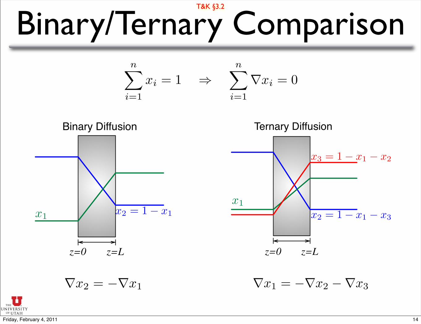
Binary/Ternary Comparison

∇x2 = −∇x1 ∇x1 = −∇x2 −∇x3

z=0 z=L

Binary Diffusion

x2 = 1− x1x1

z=0 z=L

Ternary Diffusion

x3 = 1− x1 − x2

x2 = 1− x1 − x3

x1

n�

i=1

xi = 1 ⇒n�

i=1

∇xi = 0

T&K §3.2


Fick's

Law

Ternary Diffusion

"normal"

diffusion

−∇x1

J1

Diffusion Regimes

J1 = −ctD∇x1 J1 = −ctD11∇x1 − ctD12∇x2,

J2 = −ctD21∇x1 − ctD22∇x2.

Fick's

Law

Ternary Diffusion

"normal"

diffusion

−∇x1

J1

osmotic

diffusion

Fick's

Law

Ternary Diffusion

"normal"

diffusion

−∇x1

J1

reverse

diffusion

osmotic

diffusion

Fick's

Law

Ternary Diffusion

"normal"

diffusion

−∇x1

J1

reverse

diffusion

osmotic

diffusiondiffusion

barrier

(J) = −ct[D](∇x)Fi

ck's

Law

D12

Binary DiffusionJ1

−∇x1


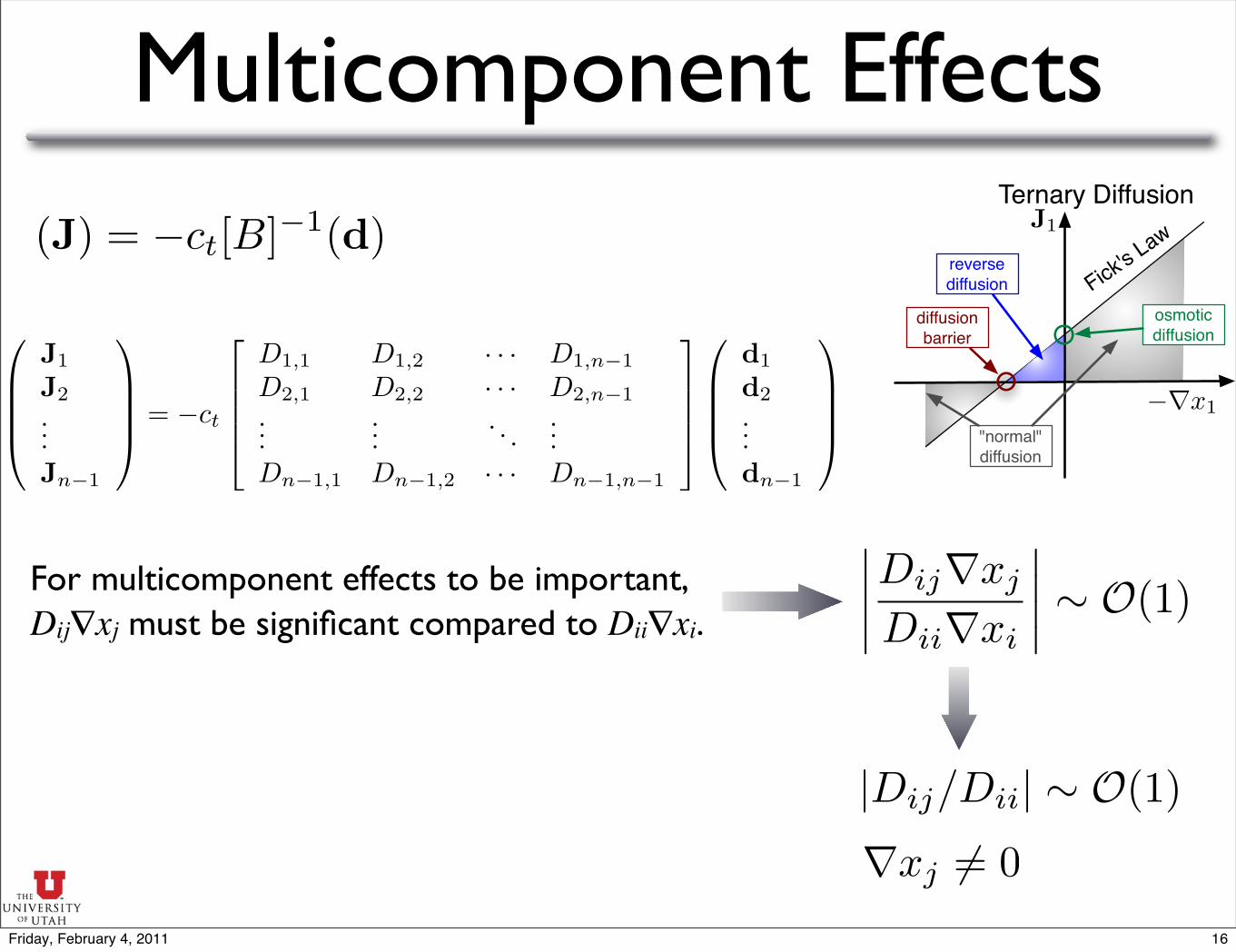
Multicomponent Effects

Fick's

Law

Ternary Diffusion

"normal"

diffusion

−∇x1

J1

reverse

diffusion

osmotic

diffusiondiffusion

barrier

J1

J2...Jn−1

= −ct

D1,1 D1,2 · · · D1,n−1

D2,1 D2,2 · · · D2,n−1...

.... . .

...Dn−1,1 Dn−1,2 · · · Dn−1,n−1

d1

d2...dn−1

(J) = −ct[B]−1(d)

For multicomponent effects to be important, Dij∇xj must be significant compared to Dii∇xi.

��Dij∇xj

Dii∇xi

�� ∼ O(1)

|Dij/Dii| ∼ O(1)

∇xj �= 016Friday, February 4, 2011

Fick’s Law & Reference VelocitiesHow do we write Fick’s law in other reference frames?

(J) = −c[D](∇x)

Mass diffusive flux relative to a mass-averaged velocity.

Molar diffusive flux relative to a molar-averaged velocity.

Molar diffusive flux relative to a volume-averaged velocity.

Option 1: Start with GMS equations and write them for the desired diffusive flux and driving force. Then invert to find the appropriate definition for [D].

Option 2: Given [D], define an appropriate transformation to obtain [D°] or [DV].

T&K §3.2.4, 1.2.1

(j) = −ρt[D◦](∇ω)

(JV ) = −[DV ](∇c)

[D◦] = [Buo]−1[ω][x]−1[D][x][ω]−1[Buo]= [Bou][ω][x]−1[D][x][ω]−1[Bou]−1

Buoik = δik − ωi

�xk

ωk− xn

ωn

�

Bouik = δik − ωi

�1− ωnxk

xnωk

�

BV uik = δik −

xi

V̄t

�V̄k − V̄n

�

BuVik = δik − xi

�1− V̄k

V̄n

�[DV ] = [BV u][D][BV u]−1

= [BV u][D][BuV ]


T&K Example 3.2.1Given [DV] for the system acetone (1), benzene (2),

and methanol (3), calculate [D].

V̄1 = 74.1× 10−6 m3

mol

V̄2 = 89.4× 10−6 m3

mol

V̄3 = 40.7× 10−6 m3

mol

V̄1 = 74.1 ! 10"6 m3

mol

V̄2 = 89.4 ! 10"6 m3

mol,

V̄3 = 40.7 ! 10"6 m3

mol

x1 x2 DV11 DV

12 DV21 DV

22

0.350 0.302 3.819 0.420 -0.561 2.133

0.766 0.114 4.440 0.721 -0.834 2.680

0.533 0.790 4.472 0.962 -0.480 2.569

0.400 0.500 4.434 1.866 -0.816 1.668

0.299 0.150 3.192 0.277 -0.191 2.368

0.206 0.548 3.513 0.665 -0.602 1.948

0.102 0.795 3.502 1.204 -1.130 1.124

0.120 0.132 3.115 0.138 -0.227 2.235

0.150 0.298 3.050 0.150 -0.269 2.250

1

(J) = −c[D](∇x) (j) = −ρt[D◦](∇ω) (JV ) = −[DV ](∇c)

[DV ] = [BV u][D][BV u]−1

= [BV u][D][BuV ]

Diffusivities in units of 10-9 m2/s

T&K §3.2.3-3.2.4


the maxwell-stefan equations - james c. sutherland 12: drag coefﬁcient for drag that particle...

Documents