it’s where you work: increases in earnings dispersion...
TRANSCRIPT

DI
SC
US
SI
ON
P
AP
ER
S
ER
IE
S
Forschungsinstitut zur Zukunft der ArbeitInstitute for the Study of Labor
It’s Where You Work: Increases in Earnings Dispersion across Establishments and Individuals in the U.S.
IZA DP No. 8437
August 2014
Erling BarthAlex BrysonJames C. DavisRichard Freeman

It’s Where You Work: Increases in Earnings Dispersion across
Establishments and Individuals in the U.S.
Erling Barth Institute for Social Research, ESOP, University of Oslo, NBER and IZA
Alex Bryson
National Institute of Economic and Social Research, CEP, LSE and IZA
James C. Davis U.S. Census Bureau, BRDC and NBER
Richard Freeman
Harvard University, NBER, CEP, LSE and IZA
Discussion Paper No. 8437 August 2014
IZA
P.O. Box 7240 53072 Bonn
Germany
Phone: +49-228-3894-0 Fax: +49-228-3894-180
E-mail: [email protected]
Any opinions expressed here are those of the author(s) and not those of IZA. Research published in this series may include views on policy, but the institute itself takes no institutional policy positions. The IZA research network is committed to the IZA Guiding Principles of Research Integrity. The Institute for the Study of Labor (IZA) in Bonn is a local and virtual international research center and a place of communication between science, politics and business. IZA is an independent nonprofit organization supported by Deutsche Post Foundation. The center is associated with the University of Bonn and offers a stimulating research environment through its international network, workshops and conferences, data service, project support, research visits and doctoral program. IZA engages in (i) original and internationally competitive research in all fields of labor economics, (ii) development of policy concepts, and (iii) dissemination of research results and concepts to the interested public. IZA Discussion Papers often represent preliminary work and are circulated to encourage discussion. Citation of such a paper should account for its provisional character. A revised version may be available directly from the author.

IZA Discussion Paper No. 8437 August 2014
ABSTRACT
It’s Where You Work: Increases in Earnings Dispersion across Establishments and Individuals in the U.S.*
This paper links data on establishments and individuals to analyze the role of establishments in the increase in inequality that has become a central topic in economic analysis and policy debate. It decomposes changes in the variance of log earnings among individuals into the part due to changes in earnings among establishments and the part due to changes in earnings within-establishments and finds that much of the 1970s-2010s increase in earnings inequality results from increased dispersion of the earnings among the establishments where individuals work. It also shows that the divergence of establishment earnings occurred within and across industries and was associated with increased variance of revenues per worker. Our results direct attention to the fundamental role of establishment-level pay setting and economic adjustments in earnings inequality. JEL Classification: J3, J31, D3 Keywords: earnings, earnings inequality, productivity Corresponding author: Alex Bryson National Institute of Economic and Social Research 2 Dean Trench Street London, SW1P 3HE United Kingdom E-mail: [email protected]
* We have benefited from support from the Labor and Worklife Program at Harvard University, NBER and from the Norwegian Research Council (project 173591/S20, Barth and Bryson). Opinions and conclusions expressed herein are those of the authors and do not necessarily represent the views of the U.S. Census Bureau. Results have been reviewed to ensure that no confidential information is disclosed.
2
The defining feature of the distribution of US earnings from the mid 1970s through the
2000s is the huge increase in inequality. Analysis of individual earnings show that inequality
increased among workers with different observed measures of skill such as education, age, and
occupation and that earnings increased more at higher percentiles than lower percentiles of the
earnings distribution even among workers with the same measured skill.1
This paper examines earnings inequality along a dimension that previous research has
largely ignored: the establishments that employ the worker. Viewing inequality through an
establishment lens, we find that most of the increased variance in earnings among individuals is
associated with increased variance of average earnings among the establishments where they
work. Our findings direct attention to the role of establishment and firm pay setting and labor
market adjustments by place of work in the rising tide of inequality.2
To analyze the effect of establishment earnings on the trend increase in inequality, we
combine several data sets: the March Current Population Surveys (CPS) files that record annual
earnings and weeks worked of individual workers; the Census Bureau's Longitudinal Business
Data Base (LBD), which is the longitudinal version of the Census business register with data on
establishment payroll and employment3; the Longitudinal Employer-Household Dynamics data
(LEHD) which contains data on the earnings of millions of workers and their place of work from
unemployment insurance files. We link the LBD and LEHD through establishment identifiers to
decompose the inequality of earnings among workers into the part that occurs between
1 See eg Autor, Katz and Kearney (2008) and Lemieux (2006). 2 Previous work on the employers’ role in wage setting include Groschen (1991), Davis and Haltiwanger (1991), Abowd et al (1999), Hellerstein et al (1999), Lane et al (2007), and Gruetter and LaLive (2009) following the early works on inter-industry wage differentials, Bell and Freeman (1991), Dickens and Katz (1987), Krueger and Summers (1998 ) and Gibbons and Katz (1992). Lazear and Shaw (2009) made the observation that across firm differences appeared to be growing over time for a significant number of countries, as for instance seen in the contribution on Sweden by Nordström Skans, Edin and Holmlund (2009) in their volume. Card et al (2013) find a growing contribution of plant heterogeneity in wages in Germany between 1985 and 2009. 3 See Jarmin and Miranda (2002).

3
establishments and the part that occurs within establishments. Since the LEHD data does not
include exact information on individuals’ education, we link individuals on the LEHD to their
responses on the 1990 and 2000 Census long-form sample and 1986-98 March CPS files to
determine workers' years of schooling4.
Section one of the paper estimates the contribution of changes in the dispersion of
average earnings across establishments to the rise in inequality. Section two connects the
distribution of establishment earnings to returns to measured skill and to the sorting of workers
by skill among establishments. Section three estimates the contribution of establishment earnings
to the growth of earnings at each percentile of the earnings distribution and to the increased gap
between top earners and other workers. Section four assesses the pathways behind the widening
distribution of establishment level earnings.
Section 1: Earnings among establishments and earnings inequality among workers
Analysis of the link between growing earnings inequality among workers and changes in
the distribution of earnings among establishments requires earnings data for individuals and
establishments and links between individual and establishment earnings. We measure individual
earnings by weekly earnings (annual earnings/ weeks worked) from the internal Census version
of the March CPS files5, and use the variance of ln weekly earnings as our measure of inequality.
The internal Census CPS has higher top codes for income and thus more accurate earnings at the
top of the distribution than publicly available files6. We measure establishment earnings by
4 Eductional codes are transformed to grade levels using Jaeger (1997) and subsequent adaptations 5 The pattern of change in ln weekly earnings resembles the pattern in the widely studied ln hourly earnings from the CPS Outgoing Rotation group files. Lemieux (2006) compares CPS-based inequality measures. 6 We use the internal Census March Current Population Survey from survey years 1978-2009 to obtain observations of weekly wages from 1977-2008. All samples include workers of age 16-64 with more than 5 hours per week last year, more than 12 weeks worked last year, and whose class of work in their longest job last year was private or government wage/salary employment. Students, agricultural employment, public administration and armed forces

4
annual earnings per worker (payroll before deductions/number of employees) in the LBD and
use the variance of ln annual earnings per worker to measure inequality7.
Panel A of Figure 1 displays estimates of the variance of ln weekly earnings for
individuals from the March CPS and the variance of ln annual earnings among establishments
from the LBD. The top line shows a substantial increase in the variance of March CPS earnings
that is comparable to increases found in other CPS-based earnings data. The middle line gives
the variance of ln average earnings among establishments, weighted by establishment
employment for comparability with the CPS variance for individuals. The variance of
establishment earnings lies below the variance of individual earnings because the establishment
variance excludes variation within establishments while the variance of individual earnings
includes the variance among establishments as well as within establishments. The bottom line
gives the residual variance from regression estimates of ln earnings on the worker characteristics
specified in the table note. Reflecting the role of human capital and demographic factors in
earnings, the residual variance lies below the unadjusted variance among individuals and below
the variance of establishment earnings as well.
are excluded. Weekly earnings are calculated as annual earnings divided by the weeks worked in the prior year. Gross earnings include wages, salaries, overtime, tips and commissions. Allocated earnings observations are excluded using the earnings allocation flags. Final weights are used in all calculations. Observations with a real wage below half the minimum wage level in 1982 were excluded. 7 The data follow the definition of salaries and wages used for calculating the federal withholding tax. They report the gross earnings paid in the calendar year to employees at the establishment prior to such deductions as employees’ social security contributions, withholding taxes, group insurance premiums, union dues, and savings bonds. Included in gross earnings are all forms of compensation such as salaries, wages, commissions, dismissal pay, paid bonuses, vacation and sick leave pay, and the cash equivalent of compensation paid in kind. Salaries of officers of the establishment, if a corporation, are included. Payments to proprietors or partners, if an unincorporated concern, are excluded. Salaries and wages do not include supplementary labor costs such as employer’s Social Security contributions and other legally required expenditures or payments for voluntary programs. The definition of payrolls is identical to that recommended to all Federal statistical agencies by the Office of Management and Budget. Wages are converted to constant 2002 dollars using the Consumer Price Index. Establishments are excluded that have an average wage less than half the yearly equivalent of the 1982 minimum wage of $3.35 an hour (CPI deflated) for a 40 hour week. Establishments with over 100,000 employees are also excluded, as from observation these are generally firm level or miscoded records, and we are not aware of a U.S. establishment that large. One issue with our wage measure is that payroll is reported annually, and employment is reported for the week of March 12. The establishment wage can be affected by significant changes in establishment employment within the year.

5
To focus attention on the similarity in changes among the three measures, figure 1B
displays the variances scaled at 0 in 1977. The 1977-2009 increase for individual earnings is
0.170 ln points. The increase in the earnings equation residuals is 0.147 ln points. These
estimates imply that 86% (0.147 points/0.170 points) of the overall trend is due to the residuals
while 14% is associated with the observables.8 The variance of establishment earnings increased
by the same 0.147 points as the variance of residuals. Thus, if we take the increased variance in
establishment earnings and the 0.023 point increase in the variance due to observable worker
attributes we get the entire increase in the variance of individual earnings. The exact accounting
is happenstance, but the calculation demonstrates our main finding: that increased variance of
establishment earnings is a major pathway of inequality9.
Given that the variances in figure 1 come from different earnings series the analysis falls
short of an ANOVA decomposition of the trend increase in inequality into its between-
establishment and within-establishment components. An ANOVA requires a single earnings
series with identifiers for individuals and establishments, which the LBD and CPS do not have.
The absence of data on the earnings of workers in establishments manifests itself in our estimate
of the variance of establishment earnings. We use the variance of the ln average establishment
earnings instead of the variance of the average ln worker earnings in an establishment
appropriate to a complete variance decomposition.
How much does this distort the calculations? To estimate the magnitude of the distortion
we applied Aitchison and Brown's (1962, p. 8) formula for the difference between the variance of
ln average establishment earnings and the variance of the average of ln earnings when data are
8 Age and education explain most of the 14% of the increased variance due to observable worker attributes. 9 See Davis and Haltiwanger (1991) and Dunne et al (2004) for early observations of this in manufacturing.

6
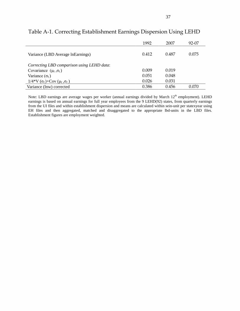
distributed log-normally10. Appendix Table A-1 estimates the differences in the two variances
and finds only modest differences in the levels of the variances and virtually identical changes in
the variances over time. As long as the log-normal assumption holds, using the variance of ln
average earnings rather than the variance of the average ln of earnings for the establishment
variance does not substantively distort the figure 1 results.
LEHD earnings
But the LEHD allows us to do better. It allows for us to link earnings to workers and to
the establishments where they work11 which is necessary to decompose the variance of ln
earnings into its between and within establishment components arithmetically. For this analysis,
we measure individual earnings by yearly earnings for workers employed in all four quarters of a
year from 1992 to 2007 in the nine states that provide such information.12
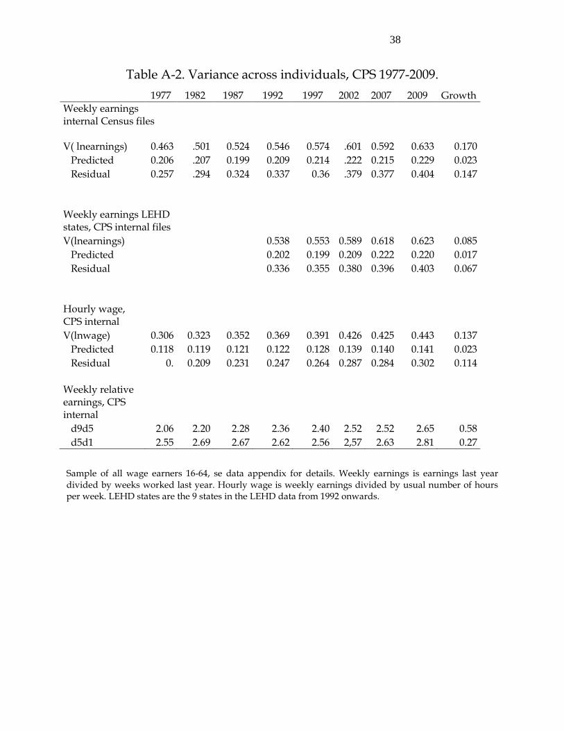
To see if the LEHD earnings are representative of the US we compared the variance of ln
yearly LEHD earnings to the variance of ln March CPS weekly earnings for the nine states. We
obtained similar levels of variance and nearly identical changes in variances.13 We then
compared the CPS variance of ln earnings in the nine states to the variance for the whole country
10 In the Appendix, we use LEHD data to adjust the variance of ln average establishment earnings to approximate the variance of the ln of average earnings using: ln E(w)= μf + σf
2/2, where μf is is σf2 is the within-
establishment variance of ln earnings. The 1992-2007 variance increase is 0.070 (adjusted) and 0.075 (unadjusted). 11 The LEHD and LBD link identifies the firm that employs workers and the establishment in which they work when firms have one establishment in a locality. When firms have multiple establishments in a locality the Census uses a probabilistic worker assignment to estimate the establishment in which the worker was employed. We use the Census's probabilistic assignment to identify the establishment location of all workers. See Abowd et al (2002, 2003, and 2007) for details and methods regarding the use of LEHD data. 12 The nine states are: California, Colorado, Idaho, Illinois, Maryland, North Carolina, Oregon, Washington, and Wisconsin. They cover nearly half of US employment. The LEHD data cover the last and first quarters of 1991 and 2008, but seasonality creates comparability problems with the annual data. 13 The LEHD variance for 1992 is 0.506 and 0.588 for 2007 (table 1). The CPS-based variance for the same states is 0.538 in 1992 and 0.618 in 2007. The increases in the LEHD-based variance (0.082) and CPS-based variance (0.080) are also nearly identical.

7
and also found similar levels and nearly identical changes.14 Thus, analysis of the LEHD should
generalize to the entire country.15
Given these assurances, we decompose the LEHD earnings into their within and between
establishment components and calculated changes in the components over time. Denote lnwip as
the ln earnings of individual i in establishment p; Elnwip as the mean ln earnings for workers in
establishment p; Vw as the within component of variance, and Vb as the between component. The
variance decomposition of ln earnings is:
(1) V(ln wip) = Vw+ Vb = V(ln wip – Elnwip) + V(Elnwip),
Table 1 records the decomposition in the nine LEHD states from 1992 to 2007. In 1992
and 2007 ln earnings varied more within establishments than between establishments. But the
increase in the between-establishment variance (0.056) is over twice the increase in the within-
establishment variance (0.027), so that the between component accounts for 67.5% of the
increased variance among all workers16. While the 67.5% estimate falls short of the 87%
estimated establishment share found in figure 1, it is further evidence of the importance of
increased inequality among establishments in the increased inequality among US workers.
Stayers
The longitudinal nature of the LEHD allows us to estimate the relation between the
dispersion in average establishment earnings and dispersion in individual earnings in another
way. This is by decomposing the change in the variance of ln earnings for a select group of 14 Appendix Table A-1b gives a CPS-based variance of ln earnings for the US of 0.546 in 1992 and 0.633 in 2009. The CPS-based variance for our nine states is 0.538 in 1992 and 0.623 in 2009. The 1992-2007 change for the US (.087) is almost identical to that for the nine LEHD states (.085). 15 We also examined the pattern of change in other states that the LEHD covered over shorter periods and found similar results to those in our sample of states. 16 The calculation is 0.056 points/0.083 points = 67%. The results are similar if we take earnings for the larger sample of workers who appear in at least a single quarter (the 2nd quarter of the year in our calculation). They are also similar for 22 states that appear in the data for a shorter time period. See appendix table A-2.

8
workers – those who stay in the same establishment one year to the next. Analysis of changes in
inequality among stayers holds fixed the time invariant unobservable and observable
characteristics of both workers and establishments. It pins down the impact of the widening
establishment earnings on individual earnings in a way that sidesteps complications due to the
connections between earnings, labor mobility, exit and entry of establishments, and matching of
workers and establishments.
To see how data on stayers illuminates the role of establishments, consider two
establishments, all of whose workers are stayers. In this case, inequality of worker earnings
could increase because of: increased earnings differentials between the establishments, with
unchanged relative earnings within establishments; increased relative earnings within
establishments, with unchanged differentials between establishments; or some mixture of
between and within-establishment changes. The decomposition for stayers arithmetically
measures the between establishment and within establishment effects on stayers inequality.
Line 1 of Table 2 gives our estimates of the change in variance of ln earnings for stayers
from year t-1 to t over specified periods. Since workers who stay at an establishment differ from
one year to the next we maximize the number of persons in the computation by using a rolling
sample. We calculated ln earnings for stayers in years t-1 and t, computed the variance in both
years and then took the change in variances from t-1 to t to measure the change in inequality. We
repeated the calculation for year t to t+1 and so forth. The 0.013 in the column labeled 1992 to
1997 sums the change in the variance of ln earnings for stayers from 1992-93 to 1996-97. The
0.024 in the 1997-2002 column sums the change in variance from 1997-98 to 2001-02. And so
forth. The estimates show moderate increases in variance in 1992-97 and 1997-02 followed by a
larger increase in 2002-07. Over the entire period the change in variance was 0.061 ln points.

9
How much of the changed variance among stayers is associated with changes in earnings
among establishments? The line “changes in between-establishment variance” estimates the
changed variance of the average ln earnings among establishments. These estimates are the sum
of the changed variance of establishment level ln earnings of stayers from one year to the next
over the specified period. They attribute all of the increased variance among stayers from 1992 to
1997 to the increased between-establishment variance (0.013 points/0.013 points) and attribute
smaller but still dominant shares of the increased variance in ensuing periods to the increase in
variance among establishments. For the whole period, the change in variance due to the changed
variance among establishments of 0.048 points is 79% of the 0.061 total increase in variance.
The remaining 21% is the contribution of changes in within-establishment variance.
The bottom part of table 2 summarizes analogous variance decompositions for all
employees. Changes in variance are larger for all employees than for stayers because all
employees are a more heterogeneous group that includes workers who move from one
establishment to another or between employment and non-employment. The variance among all
workers increases by 0.083 points, of which two-thirds (0.056/0.083) is between establishments.
Dividing the change in total variance for stayers by the change for all employees shows that the
stayers account for nearly three quarters of the increased overall variance. This reflects the fact
that most workers stay in the same job from one year to the next. While exit and entry of
establishments and movement of workers among establishments and between work and non-
work contribute to the variance, the increased variance among stayers due to changing
establishment differentials is the main driver of the trend in variance for all workers.

10
Section 2: Worker characteristics and establishment premium.
Most studies of earnings inequality focus on the contribution of increased returns to
observable characteristics such as education or age. To examine the interaction between
establishment earnings and the returns to skill and sorting of workers by skill among
establishments in the rising trend in inequality requires a valid measure of years of schooling,
which the LEHD does not provide. To obtain a measure of schooling for individuals we matched
the LEHD records to the 1990 and 2000 Census long forms and 1986-1998 March CPS files to
obtain Census or CPS years of schooling to add to the LEHD.17 We then estimated the following
extension of the standard ln earnings equation each year from 1992 to 2007:
(2) lnwip= xip b + φ p(i) + uip, with E(uip |xip, φp) = 0
In this equation xip is a vector of worker characteristics (years of schooling, experience
(Mincer), and its square, dummy variables for non-white and gender) for worker i in
establishment p. We interact the independent variables with gender to allow for male-female
differences. By omitting establishment subscripts on the b coefficient, we impose equal within-
establishment returns to characteristics and place any within-establishment heterogeneity in
returns into the error term.
Our extension of the standard ln earnings model is the vector of dummy variables φp(i)
for the establishment where the individual works. We impose equal establishment effects on
workers by omitting the individual subscript from establishment dummy variables but write the
vector as a function of i to highlight that all workers in an establishment share the same
establishment effect. This specification puts individual heterogeneity in the establishment effect,
17 The long form is distributed to approximately 15 percent of the US population every decennial. The combination
of Census long form and the CPS allows us to match 18% of the LEHD sample with those files and thus obtain valid education measures for a large number of workers. To maximize the sample with education data we match to the 2000 Census, then to the 1990 Census, and finally add information from the CPS 86-98 sample.

11
(which reflects the quality of the individual and establishment match) into the error term.
Taking the variance of (2) we decompose the variance of ln earnings into the part due to
variance of skills among workers, the variance of earnings among establishments, the covariance
between them, and the variance in the error term. To simplify the algebra, denote a worker's skill
as s (= xb, a composite that depends on worker attributes weighted by the estimated b
coefficients linking attributes to earnings) and denote V(φ) as the variance of the establishment's
effect on wages. This yields:
(3) V(ln w) = V(s) + V(φ) + 2 cov(s, φ) + V(u)
Taking S as the establishment’s average level of observable skills, we define ρ = cov(s,
S)/V(s) to measure the similarity of skills in an establishment. The ρ coefficient is Kremer and
Maskin's (1996) index of worker-worker segregation by skill across establishments. When
establishments hire workers randomly by skill, ρ = 0. When workers are perfectly sorted with
workers having similar skills, ρ = 1. We define ρφ= cov(s, φ)/V(s) to measure the extent to
which skills are related to the establishment's effect on earnings. The ρφ coefficient measures the
extent to which skill attributes are associated with the establishment effect. When firms hire
workers by skill level independently of the establishment earnings factor, ρφ = 0.
Given these definitions, the between-establishment variance divides into a part due to
sorting of workers and a part due to “pure” variation of earnings among establishments:
(4) Vb= V(s) ( ρ + 2 ρφ ) + V(φ).
where V(s) (ρ + 2 ρφ) term reflects the contribution of both forms of sorting of skills to between-
establishment variance; and where V(φ) is the variance of the establishment effect for workers
with similar measured skills independent of variation in the distribution of skills among
establishments.
12
Similarly, we decompose the within establishment part of the variance Vw into:
(5) Vw = V(s)(1- ρ) + V(u).
When establishments employ workers with the same skill, ρ = 1 and the variance of skills
contributes nothing to within-establishment variance. When establishments hire workers
irrespective of skill, ρ = 0, and the variance in the skill distribution contributes to the within-
establishment variance only.
Table 3 gives our decomposition of earnings in the matched LEHD-Census sample. The
Var(lnw) row records the variance of ln earnings. The variances for the matched sample are
similar to the Table 1 variances for the entire LEHD, with a slightly higher increase.18 The
similarity shows that the matching preserved the pattern of change in dispersion on which we
focus.
The row “skills: Var(s)” shows that the variance of skills, conditional on establishment
effects, had a negligible effect on the trend in variance. Since the education premium was
widening (Goldin and Katz, 2008), something else in the skill index must have offset its effect on
the variance. As we shall see, that something else is a fall in male/female earnings differences.
The estimated sorting coefficients examine the extent to which sorting of workers
increased. Worker-worker sorting (ρ) increased by a slight 1.3 percentage points over the 15 year
period. Worker-establishment sorting, ρφ, increased by a larger 6.5 percentage points, as
establishments with high earnings increasingly loaded up on high skill workers. But because the
sorting effect depends on the variance of skills, V(s), which fell slightly, sorting has little impact
in the decomposition.
What dominates the increased variance of establishment-level earnings is the increased
divergence of earnings among establishments. This contributes 0.057 points, or 65 percent, of the 18 An increase of 0.088 in Table 3 compared to 0.083 in Table 1

13
increased variance. In turn, the decomposition of the between-establishment effect shows that the
increased variance in the establishment effect, φp., accounts for the vast bulk (.049/.057 = 86
percent) of the increase in the between establishment variance.
Finally, the decomposition of the within establishment variance at the bottom of the table
shows that the within-establishment increase resulted largely from increased variance of the
residual in the equation – that is, to greater variance among workers with similar skills within
establishments – rather than from changes in the within-establishment skill composition.
The surprisingly small (and negative) effect of the variance of skills on the change in
dispersion of earnings both within and between establishments merits attention in light of large
increases in the estimated coefficient on education, which adds to the variance of earnings. To
understand what lies behind the small estimated skill effect, we decomposed the variance of
March CPS earnings yearly from 1977 to 2011 and calculated the contribution of worker
attributes to the overall increase in variance.
Figure 2 gives the results of this decomposition. The line for years of schooling shows
that schooling increased the variance of ln earnings as the return on years of schooling increased.
But the line for gender shows a large decline in the variance of ln earnings associated with
gender.19 From 1977 to 2011 the schooling measure added 0.07 points to the variance while the
gender measure reduced the variance by 0.06 points. Over the 1992-2007 period the more
modest upward trend in variance due to schooling is partially offset by declines in variance due
to gender, age, and the covariances as well.
19 In this calculation we included the covariance of gender with age. We made similar calculations for the matched LEHD data and obtained similar results. In that data set, adding establishment effects reduces the estimated educational wage differentials by about 20 percent, reflecting a positive sorting of high educated workers towards high paying establishments.

14
Section 3 The widening percentile distribution of earnings
Studies that focus on the entire distribution of earnings have documented that percentage
changes in earnings were larger in the higher percentiles of the distribution and were especially
large for top earners – the upper 10% or 1%, depending on the study.20
To see how establishment differentials affect changes in earnings by percentile in the
earnings distribution, we calculated LEHD percentile earnings distributions for individuals in
1992 and 2007. We assigned to each person the establishment effects of their workplace and
calculated the mean of establishment effect21 for all individuals at a given percentile. If the
distribution of earnings in 1992 had 1,000 workers at the 10th percentile, the establishment effect
for the 10th percentile would be the average of the establishment effects for the 1,000 workers.
Similarly, if the distribution of earnings in 2007 had 1,500 workers at the 10th percentile (due to
the increased work force), the establishment effect for the 10th percentile would be the average of
the establishment effects for those workers. Given these estimates, we then calculated the
increase in the average establishment effects by percentile between 1992 and 2007. If
establishment earnings were important in altering the distribution of earnings, the pattern of
change in the establishment earnings by percentile should mimic the pattern changes in the actual
earnings of workers in the percentiles.
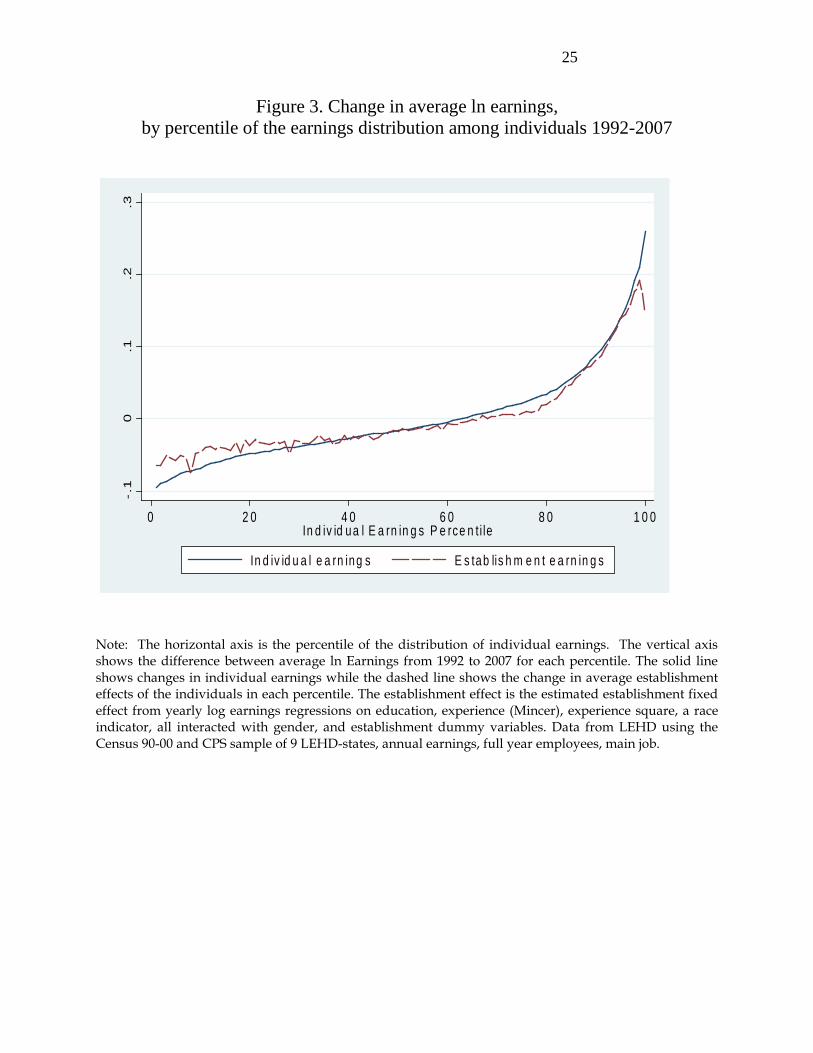
Figure 3 shows that this is the case. The dotted line gives the changes in the average
establishment effect for workers by percentile. The changes in establishment effects increase
with the percentiles of the distribution. To see how this meshes with the changes in earnings of
individuals at each percentile, we calculated the average ln earnings of individuals percentile by
percentile in 1992 and 2007 and the difference between these percentile averages. We then
20 Lemieux 2008; Alvaredo, Atkinson, Pikkety and Saez, 2013. 21 The regression includes years of schooling, experience and experience squared, a race dummy, all interacted with gender in addition to an establishment fixed effect.

15
subtracted the average change in ln earnings for all individuals from each percentiles' change. We
did this to better display similarities and differences between changes for individuals and
changes for establishment effects which, by construction average to zero with negative as well as
positive effects. Subtracting the change in the mean for individual earnings preserves relative
changes while putting individual changes in similar units as the establishment changes.
The solid line in figure 3 shows these changes. The pattern of changes for individual
earnings and for establishment effects closely mirror each other. Establishment effects have
larger increases than individual earnings at the lower end of the distribution and smaller
increases than individual earnings at the top percentiles. These differences reflect the fact that the
earnings distribution is ordered by individuals, whose changes will be influenced by their
circumstances as well as by establishment effects – individuals low in the distribution will have
negative shocks and those high in the distribution will have positive shocks. But the deviations
are modest. Changes in earnings at the establishment where people work dominate the pattern of
higher increases in earnings at higher percentiles of the distribution.
Top earners
Finally, given widespread attention to the increased relative rewards to workers at the top
of the earnings distribution, we examined the extent to which the advantage at the top increased
because earnings at the establishments at which they work increased relative to earnings at other
establishments. We divided the LEHD sample into top earners – defined as those in the upper
5% of the distribution of the nine states – and the remaining 95% . We computed the 1992-2007
increase in the ln earnings difference between the top 5% and the 95% and the impact that
increase had on earnings inequality for all workers. We then estimated the change in earnings at
16
the places where the top 5% worked relative to the 95% and the impact that had on the difference
between the 5% and the 95%.
Table 4 shows that the increased advantage of the 5% accounts for 40% of the increase in
the variance of ln earnings measures of inequality and that the divergence of establishment
earnings underlies much of the increased advantage of top earners. Line 1 records the variance
of ln earnings and change in variance for all workers in 1992 and 2007. Lines 2 and 3 estimate
the ln mean earnings and changes in ln means for the top 5% and the remaining 95%. Line 4
gives the differences in the means. The earnings advantage of the top 5% over the 95%
increased by 0.208 ln points. Line 5 uses the variance formula in the table note to calculate the
impact of the earnings gap to the total variance in each year and of the increase in the gap to the
increased variance for all workers. It gives the 40% figure cited above for the effect of the
changed gap on the total increase in variance between 1992 and 2007.22
The remainder of the table assesses the role of changes in establishment differentials on
the 0.208 increased advantage of the top 5%. Lines 6 and 7 estimate the establishment effects for
the 5% and for the 95%. The estimates follow the procedure in the figure 3 calculations just
described: they average the establishment effects from the LEHD earnings regression for all
persons in the relevant groups.23 Note that per the figure 3 discussion, the establishment effects
are scaled around zero, which places them on a different metric than the mean earnings in lines
2-4. But the changes over time are comparable. Line 8 shows that the change in the
establishment effects for the top 5% vs the 95% was 0.174. This is 84% of the change between
the mean earnings of two groups in line 4. Given that 40% of the increased variance of ln
22 The 60% of the rest of the increase in variance is due largely to increased variance in ln earnings among the 95% is associated with the widening of establishment effects in their establishments. 23 They come from the same regression of ln earnings of individuals on years of schooling, experience and experience squared, a race dummy, interacted with gender and the key vector of establishment dummies that yields the establishment effect.

17
earnings is associated with the pulling away of the top 5% versus others, the implication is that
33% (0.84 x 40%) of the increased variance of ln earnings is attributable to increased gap
between the average earnings in the establishments where the top 5% work and the average
earnings in the establishments where others work.
In sum, changes in the distribution of earnings among establishments have a huge
footprint on the change in earnings along the entire earnings distribution and on the increased
advantage of top earners compared to other workers. The question that naturally arises next is
“what forces have moved establishments further apart from each other in earnings space?”
Section 4. Pathways for the widening earnings structure among establishments
To assess the factors associated with the widening dispersion of establishment earnings
we shift the dependent variable of concern from the earnings of individuals to the average
earnings of establishments. To see what establishment-level factors might contribute to the
establishment average earnings we regressed ln average yearly earnings in establishments on
establishment attributes using the following equation:
(6) ln wp= Gp a +Ip b+ cln Ep + dMUp + e ln Efp + f lnNP + φ p
where wp is the average annual earnings in an establishment in year t from the LBD. The vector
φ p measures establishment mean earnings net of the other variables in the regression. It differs
from the establishment effects examined in sections 1-3, mainly because it does not contain
controls for skills as data on skills is not available in the LBD.
G is vector of 537 dummy variables for the geographic area in which an establishment
locates: for urban areas, it is the metropolitan area (PMSA), and for rural establishments outside
of PMSA's it is the BEA economic area.

18
I is vector for the industry in which the establishment's production fits according to the
NSAIC code, which we vary from the one (9 groups) to four digit level (277 groups)
The next set of variables reflect the size of the employing business: E is the number of
employees in the establishment, MU is a dummy for whether the establishment is a multi-unit
part of a larger firm; for those that are multi-unit Ef is employment in the firm and NP is the
number of establishments (NP) in the firm.
Table 5 summarizes the results. Each line represents a model in which we include
industry dummy variables from one digit to four digits with the final line adding employment
size variables as well. The 2007 calculations show that neither geography nor size of the
employing business contributes much to the variance in that year. What matters are industry,
whose contribution rises from 20 to 49 percent when going from one to two digit industries, then
increases modestly with additional industrial detail; and establishment effects, which represent
42 percent of the variance with detailed industry codes and employment and covariances.24
The decomposition of the change in variance from 1992 to 2007 shows that industry and
establishment also dominate changes over time. Two digit industry dummies provide
considerable information about changes in establishment earnings, but there remains
considerable variance in the changes among establishments within two digit industries. Even
with detailed four digit industry dummies, the estimated φ p vector shows substantial widening in
the distribution of earnings among establishments.
24 From 1977 to 2007 the mean number of employees in establishments increased from 18.4 to 20.0 but the standard deviation fell from 150 to 140. The mean number of employees in MU firms increased from 251.6 to 374.5, driven by increases in establishments per firm from 5.8 to 9.4; but the MU share of employment held fixed at 54%. (Based on LBD computations for 3,685,505 establishments in 1977 and 6,196,382 establishments in 2007).

19
Establishment Earnings and labor productivity
Was the increased dispersion of earnings among establishments accompanied by
increased dispersion of other measures of establishment performance or was the earnings
distribution unique in its widening?
It would be strange if earnings was the only variable that diverged among establishments.
Divergence of earnings due to the labor market factors would presumably lead establishments
with increasing wages to substitute other factors for labor – capital or innovative technology –
and raise labor productivity. At the other end of the scale, establishments with low productivity
are likely to better survive in a world where they can hire workers at wages far below average
than if wages are concentrated near the average.25 Efficiency wage models focused on the
motivational impact of wages also suggest that wages and productivity are likely to increase or
decrease together. From the productivity side, establishments in markets with inherent
heterogeneity in workplace productivity26 due to differences in the introduction of new
technology or other supply shocks or that face differential changes in product demand are likely
to see productivity increases spilling over to wages through “rent-sharing” behavior. Whatever
the causal mechanism, we expect rising dispersion in earnings to be associated with rising
dispersion of labor productivity.
As a first foray into the relation between changes in productivity and changes in
establishment earnings, we examined the link between the variance of ln revenues per worker
among establishments and the variance of ln earnings. Revenues per worker are far from an
ideal indicator of productivity but have the virtue of focusing on the flow of funds that is likely
25 Grout 1984, Moene and Wallerstein 1999, and Acemoglu 2003 examine how earnings differentials and rent sharing affects incentives to invest and implement new technology. Freeman and Kleiner (2005) show how different wage setting policies influenced the exit pattern of plants in the declining shoe industry. 26 See eg Melitz 2003, Klette and Kortum (2004), Bender et al (2008), Faggio et al (2007) and Comin et al 2009.

20
to bound labor payrolls. To estimate establishment revenues per worker, we obtained data from
the US Census Bureau's Economic Census files, which are based on quinquennial censuses of
establishments in every year with an ending of 2 or 7. 27 The upper panel of Table 6 shows the
variance of ln revenues per worker in one digit private sector industries every five years from
1977 to 2007. The lower panel of the table gives the corresponding variance of ln earnings
among establishments from the LBD. The variances of ln revenues per worker are much larger
than the variances of ln yearly earnings -- 2-3 times larger for all sectors – and increased twice as
much as the variances of ln earnings (0.311 versus 0.156). For whatever reason, in the period
under study, establishments moved further apart in revenue per worker than they did in earnings.
Rent-sharing and other non-competitive models of wage determination posit that
exogenous changes in revenues/profits change wages in the same direction28. Following this
logic we examine the link between wages and revenues using the following model:
(7) lnwpir = a + bln Rpir + c ln AW ir + d sI + vpir
where Rpir is revenue per worker in establishment p, industry i and region r, AWir is the average
wage of industry i in region r, an indicator of alternative wages that would affect wpir in the
establishment and region through supply conditions, and sI is a composite observable skills
measure at detailed industry level.29
Table 7 presents the results from estimating equation (7) on a panel of establishments for
five year intervals from 1977 to 2007. The key coefficient in the regression is the b parameter
that links revenues per worker to earnings. Given the fact that variance of revenues per worker
27 http://factfinder2.census.gov/faces/nav/jsf/pages/programs .xhtml?program=econ 28 See eg Arai (2003), Martins (2009), Dobbelaaere and Mairesse (2008) and Card et al (2013) for empirical evidence. 29 The skills measure is the average predicted xb from the section 1 equations using the yearly CPS files, where x includes education, experience and its square, all interacted with gender. We averaged the skill measure by detailed industry using the definition of ind50 from the IPUMs to match each year to sic3 and naics4. See data appendix.

21
increased at about twice the variance of earnings, an estimated b of around 0.7 would attribute
most of the increased variance of ln earnings to the increased variance of revenues per worker.30
None of our estimated models give such a large rent sharing parameter. The OLS model in
column 1 has a rent sharing parameter of 0.386. Addition of establishment fixed effects in
column 2 (so that the analysis links within establishment earnings to within-establishment
revenues per worker) drops the rent-sharing parameter to 0.324. The instrumental variable
estimate in column 3, which deals with the endogeneity of revenues per worker by the Card,
Devicienti, and Maida (2010) method of taking revenues outside of the region of the observed
establishment as the instrument, gives an estimate of 0.163. The identifying restriction in this
analysis is that, conditional on average earnings in the industry and region, higher revenues per
worker in the industry outside the region affects earnings solely through establishment revenues.
With an impact on earnings of 0.163 the increased revenue per worker adds about 5-6% to the
variance of earnings among establishments31 and thus falls far short of explaining the increased
variance of establishment effects and increased inequality of individual earnings. Factors beyond
demand-driven rent-sharing would seem to be needed to account for the divergence of
establishments in earnings space.
5. Conclusion
The distribution of earnings across establishments widened markedly during the 1970s-
2000s period of increasing inequality of individual earnings. Using several data sets and
modeling procedures we find that the widening of the establishment earnings distribution
30 The variance (var) decomposition of (7) links Δ var ln earnings to b2 Δ var ln revenues per worker, all else the same. With Δ var ln revenues per worker about twice the magnitude of Δ var ln earnings, b~.7 would give the b2 ~ ½ necessary for the changed variance in revenues to account for the changed variance in earnings 31 Assuming that the variance of revenues per worker increased by twice the increased variance in ln earnings the
contribution of the increase in revenues per workers would be (.163)2 (2) = .054

22
underlies much of the increase in inequality. The widening establishment distribution accounted
for most of the increased variance of ln earnings among workers, most tellingly accounting for
79 percent of the increase among stayers – workers who continued from one year to the next in
the same establishments. It also accounted for most of the pattern of larger increases in earnings
among workers higher in the earnings distribution and for most of the increased gap between
earners in the upper 5% and others. The distribution of ln revenues per worker also widened
over the period though our demand-driven rent-sharing model did not add much to the change in
variance of earnings.
In short, the pattern of change in pay and potentially other economic outcomes in the
establishments where people work has been a major factor in the much-heralded increase in
inequality. We have shown that establishments matter but have only scratched the surface of
analyzing the economics that have pulled establishments apart in earnings space. Our results
suggest the value of renewed analysis of establishment pay setting and hiring policies on the
demand side and on establishment-level mobility on the supply side, and on factors beyond
establishment demand shocks, such as productivity shocks associated with the introduction of
innovative products or processes, in producing the divergence of establishment earnings. The
huge role of establishment factors in the trend rise in inequality documented in this study is a
signpost to pay attention to the places where people work as well as to their skills in studies of
inequality.

23
Figure 1. Variance of ln(earnings) individuals and establishments, 1977-2009
Panel A: Actual Variances
.2.3
.4.5
.6
1 9 7 7 1 9 8 2 1 9 8 7 1 9 9 2 1 9 9 8 2 0 0 2 2 0 0 7ye a r
Ind iv id u a l ln ( W ) , C P S E s ta b l. ln (a v g W ), L B DInd iv id u a l re s id u a l w a g e , C P S
Panel B: Variances Scaled at zero in 1977
0.0
5.1
.15
.2
1 9 7 7 1 9 8 2 1 9 8 7 1 9 9 2 1 99 7 2 0 0 2 2 0 0 7ye a r
In d iv id ua l ln (W ) C P S E s ta b lis h m e n t ln (a v g .W ) L B DR e s id u a l W a g e C P S
Note: The variance of ln(weekly earnings) calculated over individuals from the Current Population Surveys (CPS-March) and over establishments’ average wages from the Longitudinal Business Register Data (LBD) (employment weighted). CPS residual wage is calculated from yearly regressions of individual ln(weekly earnings) on years of education, experience (Mincer), experience squared, and a race dummy, all interacted with gender. See data appendix for details and table A1 for CPS results for the LEHD states, weekly versus hourly earnings, and for measures of relative wages (d9/d5 and d5/d1). LBD data are detailed further below.

24
Figure 2. Variance decomposition of ln(earnings) from CPS,1977-2011 based on estimated impacts of individual characteristics from yearly regressions
0
.05
.1
1 9 7 7 1 9 8 2 1 98 7 1 9 9 2 1 9 9 7 2 00 2 2 0 0 7ye a r
E d u ca t io n G en d e rE x p e r ie nc e N on -w h it eC o v a r ia n ce s
Note: Calculated from yearly regressions of individual ln(weekly earnings) on years of education, experience, experience squared, and a non-white dummy, all interacted with gender. Each component consists of the sum of the gender specific terms. The “Gender” line includes the gender dummy and the covariance between age and gender, and the line labelled “Covariances” summarizes the remaining covariance terms.
25
Figure 3. Change in average ln earnings, by percentile of the earnings distribution among individuals 1992-2007
-.1
0.1
.2.3
0 2 0 4 0 6 0 8 0 1 0 0In d iv id ua l E a rn in g s P e rce n t i le
In d iv id u a l e a rn ing s E s tab lis h m e n t e a rn in g s
Note: The horizontal axis is the percentile of the distribution of individual earnings. The vertical axis shows the difference between average ln Earnings from 1992 to 2007 for each percentile. The solid line shows changes in individual earnings while the dashed line shows the change in average establishment effects of the individuals in each percentile. The establishment effect is the estimated establishment fixed effect from yearly log earnings regressions on education, experience (Mincer), experience square, a race indicator, all interacted with gender, and establishment dummy variables. Data from LEHD using the Census 90-00 and CPS sample of 9 LEHD-states, annual earnings, full year employees, main job.

26
Table 1. Level and Changes in Variance in Ln Earnings Between and Within Establishments, 9 LEHD states 1992-2007
1992 2007 Growth Variance across individuals, total 0.480 0.563 0.083 Between establishments 0.219 0.275 0.056 Within establishments 0.260 0.287 0.027 # of individuals (millions) 19.0 26.0 # of establishments (millions) 1.33 1.81 Note: The 9 LEHD states are: California, Colorado, Idaho, Illinois, Maryland, North Carolina, Oregon, Washington, and Wisconsin. Annual earnings, full year employees, main job. Results for quarterly earnings for all individuals observed at the employer in the 2nd quarter, as well as figures including 22 states for shorter periods of time, show similar patterns and are available from the authors on request.

27
Table 2. Growth in variance components within and between establishments. Stayers and all employees, LEHD data 1992-2007
Period of Change 1992-1997 1997- 2002 2002- 2007 1992- 2007 Stayers Change in Var(lnearnings) 0.013 0.011 0.037 0.061 Change in Between variance 0.013 0.008 0.027 0.048 Change in within variance 0.001 0.003 0.009 0.013
All employees Var(lnearnings) 0.023 0.020 0.040 0.083 Between 0.015 0.012 0.029 0.056 Within 0.007 0.009 0.011 0.027 Note: The table shows the accumulated growth in the variance of ln(earnings) each five years from 1992. The first panel shows the accumulated change calculated on year-to-year stayers only, the second shows growth for all.

28
Table 3. Variance Decomposition of LEHD Earnings with Individual Characteristics
1992 1997 2002 2007 92-07 Change
Share of Change
All: Var(lnw) 0.457 0.478 0.500 0.545 0.088 1.00 Skills: Var (s) 0.108 0.101 0.101 0.101 -0.007 -0.08 Worker-worker: ρ 0.344 0.340 0.345 0.357 0.013 Worker-estab.: ρ φ 0.233 0.242 0.258 0.297 0.065 Var between 0.235 0.246 0.259 0.292 0.057 0.65 Estab effect: V(φ) 0.147 0.162 0.172 0.196 0.049 0.56 Skills contrib: V(s)*ρ 0.037 0.035 0.035 0.036 -0.001 -0.01 Match contrib.: V(s)*2ρφ 0.050 0.049 0.052 0.060 0.010 0.11 Var within 0.223 0.232 0.241 0.253 0.031 0.35 Within residual: V(u) 0.152 0.165 0.174 0.189 0.037 0.42 Skills contrib.: V(s)(1-ρ) 0.071 0.067 0.066 0.065 -0.006 -0.07 # of individuals (millions) 3.9 4.2 4.3 4.3 # of establish. (millions) 0.7 0.8 0.8 0.8 ` Note: Estimated on the matched Census LEDH sample, including Decennial 1990, 2000, and the CPS sample from the 9 LEHD states (see table 1). Skills (s=Xβ) includes experience (Mincer), experience sq., years of education, and a non-white dummy, interacted with gender. Employer identification is employer-state-id-unit (sein-unit). Earnings is obtained from the LEHD data, annual earnings, full year employees, main job while education, age and race are obtained from the Census-long-form and CPS.

29
Table 4: Effect of Increase in Top 5% Earners/Other Earners Gap to Inequality and of Increased Establishment Differentials on Top 5% /other earners gap
Contribution of Earnings Gap between upper to Variance
1992 2007 Change
1. Variance of ln Earnings, all workers 0.480 0.563 0.083 2. Mean, ln earnings, upper 5% 7.843 8.142 0.299 3 Mean, ln earnings lower 95% 6.261 6.352 0.191 4. Difference in Means ( (2)-(3) ) 1.582 1.790 0.208 5. Contribution of Difference in Means to Variance
0.119 0.152 0.033 (40% of row 1)
Impact of Establishment effects
6. Establishment effects, 95th percentile 0.465 0.630 0.165 7. Establishment effects, below 95th percentile -0.024 -0.033 -0.009 8. Difference in Estab. Effects ( (6)-(7) ) 0.489 0.663 0.174 (84% of row 4) Note: Data from the 9 LEHD states 1992-2007. The contribution of the difference in means follows arithmetically from decomposing the variances of ln earnings into differences in the means between the two groups and the variances within the groups. If E(5%) is the mean ln earnings of the top 5% and E(95%) is the mean ln earnings of the remaining 95% and V(5%)is the variance of ln earnings within the top 5% and V(95%) is the variance of ln earnings within the remaining 95%, the variance of ln earnings for all workers V decomposes into (.95)(.05) (E5% - E95%)2 + 0.95 V(95%) +.05(V(5%).

30
Table 5 Variance and Growth in Variance Decompositions
Establishment level earnings Different industry detail. Dependent variable: ln(establishment wage). LBD data. Level 2007 Geo Indus Establ. 2*Cov(I;G) Empl 2*Cov(E;I,G) 1 dgt Ind (sic) 0.05 0.20 0.75 0.00 2 dgt Ind 0.04 0.49 0.52 0.01 3 dgt Ind 0.04 0.49 0.46 0.01 4 dgt Ind 0.04 0.52 0.43 0.01 4 dgt + Empl 0.03 0.52 0.42 0.01 -0.01 0.03 Change 77-07 Geo Indus Establ. 2*Cov(I;G) Empl 2*Cov(E;I.G) 1 dgt Ind (sic) 0.04 0.23 0.72 0.00 2 dgt Ind 0.03 0.49 0.43 0.01 3 dgt Ind 0.03 0.49 0.44 0.01 4 dgt Ind 0.03 0.52 0.41 0.01 4 dgt + Empl 0.03 0.52 0.40 0.04 0.00 0.01 Note: The table shows the share of variance (change in variance) attributed to the various factors, based on regression analysis of ln(establishment average wage). Geography is defined as PMSA and outside of the PSMA’s, BLS working area within state is used. The number of geographic units is 537. The number of digits refers to SIC – classification (after 1998, industries are classified according to NAICS, 6, 4,3,2,1 digits). Employment includes establishment size, firm size, the number of establishments of the firm and a dummy for multi unit firm. The establishment factor is the residual from each regression, and is thus not allowed to covary with the other factors.

31
Table 6. Variance of Revenues Per Worker and Earnings Per Worker, 1977-2007
1977 1982 1987 1992 1997 2002 2007 Change, 77-07
Var ln revenues per worker
All sectors 0.954 0.965 0.949 1.020 1.113 1.126 1.265 0.311 Mng. Util. Transp. 0.421 0.463 0.670 0.821 0.860 0.827 0.967 0.546 Manufacturing 0.593 0.633 0.638 0.656 0.686 0.646 0.742 0.149 Trade 1.135 1.129 1.115 1.165 1.228 1.207 1.280 0.145 FIRE 0.911 0.917 1.222 1.075 1.244 1.190 1.432 0.521 Personal services 0.444 0.426 0.471 0.459 0.531 0.565 0.593 0.149 Business Services 0.878 0.852 0.914 0.923 1.083 1.089 1.116 0.238 Communication 0.444 0.430 0.522 0.748 0.718 0.736 0.854 0.410 Health, Educ. Soc. 0.316 0.559 0.390 0.402 0.448 0.567 0.534 0.218 Var. ln earnings All sectors 0.332 0.362 0.412 0.413 0.443 0.446 0.488 0.156 Mng. Util. Transp. 0.302 0.317 0.328 0.327 0.323 0.313 0.316 0.014 Manufacturing 0.187 0.204 0.220 0.218 0.234 0.226 0.239 0.052 Trade 0.340 0.353 0.388 0.390 0.415 0.413 0.423 0.083 FIRE 0.202 0.303 0.433 0.447 0.467 0.516 0.579 0.377 Personal services 0.364 0.386 0.408 0.296 0.321 0.338 0.370 0.006 Business Services 0.478 0.506 0.551 0.547 0.581 0.582 0.634 0.156 Communication 0.214 0.269 0.299 0.355 0.383 0.474 0.485 0.271 Healt, Educ. Soc. 0.247 0.229 0.262 0.249 0.249 0.236 0.270 0.023
Note: ln Revenues per worker taken from the Economic Census. ln Earnings is taken from the Longitudinal Business Data base. Figures for all sectors from the Economic Census are based on the sectors available in the table every census year. The economic census expanded in scope over the 1977-2002 period but the business register and LBD covered all industries throughout. As a check, we calculated the variance of revenues per worker restricted to industries where in each year total industry employment in the economic census is greater or equal 90% of total industry employment in the LBD. The variance trend is very similar, where for 1977 the variance is 0.945, for 1982 0.965, 1987 0.991, 1992 1.036, and 1997 1.111. where the difference is calculated from the first available year in the table

32
Table 7 Establishment wage regressions Dependent variable: ln(establishment wage)
OLS
Fixed estab eff.
Fixed estab eff IV specification
ln(Sales/Employees) 0.386 0.324 0.163 (0.000) (0.000) (0,002) Skills in industry: ln(Predicted industry wage) 0.553 0.051 0.062 (0.001) (0.002) (0,002) Alternative wage: ln(Industryxregion average) 0.343 0.113 0.131 (0.001) (0.001) (0.002) 1 digit Industry controls Y - - Fixed establishment effects - Y Y 7188373 7188373 7057563 Note: The model is estimated on a panel of establishments from 1977 to 2007, quinquennial observations from the Economic Census. The models include controls for observation year and establishment age. Predicted industry wage is calculated from an ln earnings equation including years of education, experience, expeience squared, interacted with gender, averaged at the industry level using yearly CPS data. Instrumental variable (IV) specifications use industry revenue per worker, averaged over all regions except own region, as instrument for revenue per worker.

33
References Abowd, John, John Haltiwanger, Julia Lane, Kevin L. McKinney, and Kristin Sandusky (2007), “Technology and the Demand for Skill: An analysis of within and between firm differences,” NBER Working Paper 13043, April 2007. Abowd, John M., Bryce E. Stephens & Lars Vilhuber & Fredrik Andersson & Kevin L. McKinney & Marc Roemer & Simon Woodcock, (2002). "The LEHD Infrastructure Files and the Creation of the Quarterly Workforce Indicators," Longitudinal Employer-Household Dynamics Technical Papers 2002-05, Center for Economic Studies, U.S. Census Bureau Abowd, John M., Paul A. Lengermann, and Kevin L. McKinney (2003), “The Measurement of Human Capital in the U.S. Economy,” U.S. Census Bureau, Technical Paper TP-2002-09, March 2003. Abowd, John M., Francis Kramarz and David N. Margolis, (1999) "High Wage Workers and High Wage Firms," Econometrica, Econometric Society, vol. 67(2), pages 251-334, March. Acemoglu, Daron (2003) “Labor- and Caøpital-Augmenting Technical Change” Journal of European Economic Association . Vol(1):1-37. Alvaredo, Facundo & Anthony B. Atkinson & Thomas Piketty & Emmanuel Saez, 2013. "The Top 1 Percent in International and Historical Perspective," Journal of Economic Perspectives, American Economic Association, vol. 27(3), pages 3-20, Summer Andersson, Fredrik, Clair Brown, Benjamin Campbell, Hyowook Chiang, and Yooki Park (2008), “The Effects of HRM Practices and R&D Investment on Worker Productivity,” in S. Bender, J. Lane, K.L. Shaw, F. Andersson, and T. von Wachter (eds.) The Analysis of Firms and Employees: Quantitative and Qualitative Approaches, University of Chicago Press. Arai, Mahmood, (2003) “Wages, Profits and Capital Intensity: Evidence from Matched Worker-Firm Data”, Journal of Labor Economics, vol 21, 2003. Autor, David H., Lawrence F. Katz, and Melissa S. Kearney (2008), “Trends in U.S. Wage Inequality: Revising the Revisionists,” Review of Economics and Statistics, 90(2), pages 300-323. Bell, Linda and Richard Freeman (1991) The causes of rising interindustry wage dispersion in the United States Industrial and Labor Relations Review, 1991, vol. 44, issue 2, pages 275-287 Bender, Stefan, Julia Lane, Kathryn Shaw, Fredrik Andersson and Till von Wachter , eds. (2008) The Analysis of Firms and Employees, Quantitative and Qualitative Approaches, The University of Chicago Press. Card, David, Fransisco Devicienti, Agata Maida (2010), “Rent-sharing, holdup, and wages: Evidence from matched panel data”. NBER working paper 16192.
34
Card, David , Jörg Heining and Patrick Kline (2013), "Workplace Heterogeneity and the Rise of West German Wage Inequality," The Quarterly Journal of Economics, Oxford University Press, vol. 128(3), pages 967-1015. Comin, Diego, Erica L. Groshen, Bess Rabin (2006) “Turbulent Firms, Trubulent Wages?” NBER Working paper #12032. Davis, Steve J. and John Haltiwanger (1991), “Earnings dispersion between and within U.S. Manufacturing Establishments, 1963-86,” Brookings Papers on Economic Activity, Brookings Institution Press, vol.1991, pages 115-180. Dobbelaaere, Sabien and Jacques Mairesse (2008) “Micro-evidence on rent sharing from different perspectives”, working paper, CREST. Dunne, Timothy, Lucia Foster, John Haltiwanger, and Kenneth R. Troske (2004) “Wage and Productivity Dispersion in U.S. Manufacturing: The role of computer investment.” Journal of Labor Economics, University of Chicago Press, vol. 22(2), pages 397-430 Dickens, William T., and Lawrence F. Katz, "Inter-Industry Wage Differences and Industry Characteristics", in Lang, Kevin, and Jonathan Leonard, Unemployment and the Structure of Labor Markets (Oxford, UK: Basil Blackwell, 1987) Faggio, Giulia, Salvanes, Kjell and Van Reenen, John (2007) “The Evolution of Inequality in Productivity and Wages: Panel Data Evidence”, NBER Working Paper #13351 Foster, Lucia, Haltiwanger, John and Krizan, C. J. (2002) “The Link Between Aggregate and Micro Productivity Growth: Evidence from Retail Trade”, NBER Working Paper #9120 Freeman, Richard B., and Kleiner, Morris M. (2005) “The Last American Shoe Manufacturers. Decreasing Productivity and Increasing Profits in the Shift from Piece Rates to Continuous Flow Production”, Industrial Relations, Vol. 44, No. 2, pp. 307-330 Gibbons, Robert and Larry Katz (1992): Does Unmeasured Ability Explain Interindustry Wage Differentials?, Review of Economic Studies 59: 515-535. Goldin, Claudia and Lawrence Katz (2008), “The Race between Education and Technology” Harvard University Press Groschen, Erica (1991): “Sources of Intra-Industry Wage Dispersion: How Much Do Employers Matter?”, Quarterly Journal of Economics 106: 869-884. Grout, P. (1984). Investment and wages in the absence of binding contracts: a Nash bargaining approach. Econometrica 52, 449–60. Gruetter M and R. LaLive. (2009) “The Importance of Firms in Wage Setting,” Labour Economics 16(2), 149-60

35
Haltiwanger, John C., Lane, Julia I., and Speltzer, James R. (2007) "Wages, Productivity, and the Dynamic Interaction of Businesses and Workers”, Labour Economics, vol. 14(3), pages 575-602 Hellerstein, Judith K., David Neumark, and Kenneth R. Troske (1999), “Wages, Productivity, and Worker Characteristics: Evidence from Establishment-Level Production Functions and Wage Equations,” Journal of Labor Economics, 178(3):409-446. Jaeger, David A. (1997) “Reconciling educational attainment questions in the CPS and the census“ Monthly Labor Review August 1997: 36-40. Jarmin, Ron and Miranda, Javier (2002) The Longitudinal Business Database, 02-17, Center for Economic Studies, U.S. Census Bureau Klette, Tor Jakob and Samuel Kortum, 2004."Innovating Firms and Aggregate Innovation," Journal of Political Economy, University of Chicago Press, vol. 112(5), pages 986-1018, October. Krueger, Alan B., and Lawrence, H. Summers 1988. “Efficiency Wages and the Inter-Industry Wage Structure.” Econometrica 56(2): 259–94. Lane, Julia I., Laurie A. Salmon, and James R. Spletzer (2007), “Establishment wage differentials,” Monthly Labor Review, 130(4):3-17 Lazear, Edward and Kathryn Shaw, eds. (2009) The Structure of Wages: An International Comparison, The University of Chicago Press, Lemieux, Thomas (2008) "The changing nature of wage inequality," Journal of Population Economics, Springer, vol. 21(1), pages 21-48, January. Lemieux, Thomas (2006) “Increasing Residual Wage Inequality: Composition Effects, Noisy Data, or Rising Demand for Skill?” American Economic Review vol 96(3):461-498 Mairesse, Jacques and Nathalie Greenan “Using Employee Level Data in a Firm Level Econometric Study” NBER Working Paper No. 7028 March 1999 Margolis, David N. & Salvanes, Kjell G., 2001. "Do Firms Really Share Rents with Their Workers?," IZA Discussion Papers 330, Institute for the Study of Labor (IZA Martins, Pedro (2009) "Rent sharing before and after the wage bill," Applied Economics, vol. 41(17), pages 2133-2151 Melitz, Marc J. (2003) "The Impact of Trade on Intra-Industry Reallocations and Aggregate Industry Productivity," Econometrica, Econometric Society, vol. 71(6), pages 1695-1725, November. Moene, Karl Ove and Michael Wallerstein (1997) “Pay Inequality” Journal of Labor

36
Economics,Vol 15(3):403-30. Nordstöm Skans, Oskar, Per-Anders Edin and Bertil Holmlund (2009) “Wage Dispersion Wtihin and Between Plants: Sweden 1985-2000” in Lazear E P and K L Shaw (eds) The Structure of Wages: An international Comparison. University of Chicago Press.
37
Table A-1. Correcting Establishment Earnings Dispersion Using LEHD
1992 2007 92-07 Variance (LBD Average lnEarnings) 0.412 0.487 0.075 Correcting LBD comparison using LEHD data: Covariance (μf ,σf ) 0.009 0.019 Variance (σf ) 0.051 0.048 1/4*V (σf )+Cov (μf ,σf ) 0.026 0.031 Variance (lnw) corrected 0.386 0.456 0.070 Note: LBD earnings are average wages per worker (annual earnings divided by March 12th employment). LEHD earnings is based on annual earnings for full year employees from the 9 LEHD(92) states, from quarterly earnings from the UI files and within establishment dispersion and means are calculated within sein-unit per statexyear using EH files and then aggregated, matched and disaggregated to the appropriate lbd-units in the LBD files. Establishment figures are employment weighted.
38
Table A-2. Variance across individuals, CPS 1977-2009. 1977 1982 1987 1992 1997 2002 2007 2009 Growth Weekly earnings internal Census files
V( lnearnings) 0.463
.501 0.524 0.546 0.574
.601 0.592 0.633 0.170 Predicted 0.206 .207 0.199 0.209 0.214 .222 0.215 0.229 0.023 Residual 0.257 .294 0.324 0.337 0.36 .379 0.377 0.404 0.147 Weekly earnings LEHD states, CPS internal files V(lnearnings) 0.538 0.553 0.589 0.618 0.623 0.085 Predicted 0.202 0.199 0.209 0.222 0.220 0.017 Residual 0.336 0.355 0.380 0.396 0.403 0.067 Hourly wage, CPS internal V(lnwage) 0.306 0.323 0.352 0.369 0.391 0.426 0.425 0.443 0.137 Predicted 0.118 0.119 0.121 0.122 0.128 0.139 0.140 0.141 0.023 Residual 0. 0.209 0.231 0.247 0.264 0.287 0.284 0.302 0.114 Weekly relative earnings, CPS internal d9d5 2.06 2.20 2.28 2.36 2.40 2.52 2.52 2.65 0.58 d5d1 2.55 2.69 2.67 2.62 2.56 2,57 2.63 2.81 0.27 Sample of all wage earners 16-64, se data appendix for details. Weekly earnings is earnings last year divided by weeks worked last year. Hourly wage is weekly earnings divided by usual number of hours per week. LEHD states are the 9 states in the LEHD data from 1992 onwards.