jackass actions 20140114 for website
DESCRIPTION
Jackass ACTIONS 20140114 for WebsiteTRANSCRIPT
AAccttiioonn
SSeeccttiioonn

2
Introduction
This Action Section is a supplement to the book Jackass
Investing. In this section I present specific trading strategies
that exploit many of the behaviors engaged in by people who
gamble their money by believing in – and placing their money
on – the myths exposed in the book. Then in the Action Section
for the final myth, “Myth #20 – There is No Free Lunch,” I
show how you can combine these trading strategies into a “Free
Lunch” portfolio. As you learned in the book, a Free Lunch
portfolio is one that produces both greater returns and less risk
than conventional portfolios.
The trading strategies presented in this section vary in
complexity and the commitment required by you to capture
their returns. While the returns from some of them can be
captured simply by investing in mutual funds or ETFs that are
managed pursuant to the trading strategies, others require you
to actively monitor and potentially trade them on a day-to-day
basis.
Because of this varying complexity and my interest in making
the book and this Action Section beneficial to all investors, I
present two categories of Free Lunch portfolios. These are the
“Regular” Free Lunch portfolio that incorporates all of the
trading strategies, and the “Simplified” Free Lunch portfolio
that eliminates the trading strategies that require day-to-day
monitoring.
The trading strategies presented in this section are by no
means intended to be comprehensive. But they do represent a
good cross-section of strategies that can be employed to better
diversify your portfolio across multiple return drivers. This
process results in true portfolio diversification (in contrast with
the “illusory” diversification preached by conventional financial

Action – Introduction 3
wisdom), and is the basis for the creation of your Free Lunch
portfolio.
Despite the fact that I present the historical performance of
many of these trading strategies, either in this section or in the
myth, that performance is often hypothetical, in that no single
account may have traded pursuant to each strategy or during
the period for which its performance is displayed. While many
of the trading strategies were developed prior to the start of
their displayed performance, others were developed more
recently and their historical performance is solely the result of
back-testing. Because of this the disclaimer that PAST
PERFORMANCE IS NOT INDICATIVE OF FUTURE
PERFORMANCE, which you see displayed on virtually all
investment marketing materials, holds true for each of these
trading strategies, as it does for any investment.

Contents
Introduction ........................................................................................................ 2
Action – Myth #1 Stocks Provide an Intrinsic Return ................................. 5
Action – Myth #3 You Can’t Time the Market .......................................... 19
Action – Myth #4 “Passive” Investing Beats “Active” Investing .............. 27
Action – Myth #6 Buy Low, Sell High ......................................................... 34
Action – Myth #7 It’s Bad to Chase Performance ...................................... 45
Action – Myth #8 Trading is Gambling – Investing is Safer ..................... 50
Action – Myth #10 Short Selling is Destabilizing and Risky ...................... 53
Action – Myth #11 Commodity Trading is Risky........................................ 57
Action – Myth #12 Futures Trading is Risky .............................................. 59
Action – Myth #14 Government Regulations Protect Investors ................ 64
Action – Myth #15 The Largest Investors Hold All the Cards................... 67
Action – Myth #16 Allocate a Small Amount to Foreign Stocks ................ 70
Action – Myth #20 There is No Free Lunch ................................................ 76

5
Action – Myth #1
We saw in Myth #1 how people’s sentiment towards buying and
selling stocks, rather than actual corporate performance,
dominates short-term stock performance. The trading strategy
I present here is designed to capitalize on this return driver.
The strategy buys the stocks of good companies when they are
being shunned by others and attempts to ride prices higher as
sentiment improves. Best yet, the strategy is time-tested with
more than a decade of actual market performance. Because this
trading strategy generally produces portfolios that contain less
than 10 stocks, it is suitable for both small and large portfolios.
Discovering Piotroski
In 2001 I launched a market neutral equity fund that held a
portfolio of about 100 U.S. exchange traded stocks each long
and short and also utilized a variety of trading strategies. One
of the strategies we employed was an adaptation of a trading
strategy developed by Joseph Piotroski, at the time an
accounting professor at the University of Chicago Graduate
School of Business. Piotroski’s strategy combined value
measures, such as price to book ratio, with financial
performance, such as profitability and cash flow. Not only did
Piotroski’s trading strategy perform well when tested against
historical stock market data, it has continue to perform well in
real-time since its release to the public more than ten years
ago. Let’s take a look.
Piotroski Performance
Piotroski tested his strategy across 21 years of historical data
(1976 – 1996). In that back-testing Piotroski’s strategy
outperformed the market by an average of 13.4% per year.
Those results, of course, had the benefit of hindsight. Meaning
that the strategy had been developed to perform well on that
6 Jackass Investing – Action for Myth #1
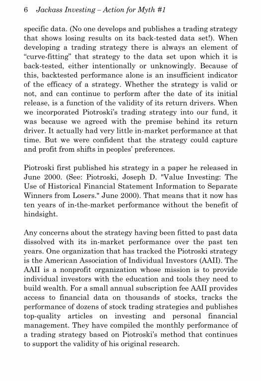
specific data. (No one develops and publishes a trading strategy
that shows losing results on its back-tested data set!). When
developing a trading strategy there is always an element of
“curve-fitting” that strategy to the data set upon which it is
back-tested, either intentionally or unknowingly. Because of
this, backtested performance alone is an insufficient indicator
of the efficacy of a strategy. Whether the strategy is valid or
not, and can continue to perform after the date of its initial
release, is a function of the validity of its return drivers. When
we incorporated Piotroski’s trading strategy into our fund, it
was because we agreed with the premise behind its return
driver. It actually had very little in-market performance at that
time. But we were confident that the strategy could capture
and profit from shifts in peoples’ preferences.
Piotroski first published his strategy in a paper he released in
June 2000. (See: Piotroski, Joseph D. "Value Investing: The
Use of Historical Financial Statement Information to Separate
Winners from Losers." June 2000). That means that it now has
ten years of in-the-market performance without the benefit of
hindsight.
Any concerns about the strategy having been fitted to past data
dissolved with its in-market performance over the past ten
years. One organization that has tracked the Piotroski strategy
is the American Association of Individual Investors (AAII). The
AAII is a nonprofit organization whose mission is to provide
individual investors with the education and tools they need to
build wealth. For a small annual subscription fee AAII provides
access to financial data on thousands of stocks, tracks the
performance of dozens of stock trading strategies and publishes
top-quality articles on investing and personal financial
management. They have compiled the monthly performance of
a trading strategy based on Piotroski’s method that continues
to support the validity of his original research.

Action – Myth #1 7
Impressively, from January 2001 through year-end 2009 the
strategy produced a 29% average annualized return. As I
prepared to publish this book its performance virtually
exploded, bringing the average annual return to 48% by the
end of 2010. The strategy produced these returns at a time
when most people were merely trying to avoid substantial
losses. This performance helps to confirm the research that
shows that sentiment is a key driver of short-term stock
performance.
Figure 1 and Figure 2 display the performance of this strategy
beginning January 2001 (subsequent to its publication). The
returns include a cost of 4% each year to account for the
transaction costs that could have been incurred in actual
trading.
Note 1-1: As of January 2011, transaction costs are assumed to
be 0.50% per transaction.

8 Jackass Investing – Action for Myth #1
Growth in $1,000
Allocated to Piotroski Trading Strategy On January 1, 2001
Piotroski-based Trading Strategy Annual Returns
Figure 1. Source: AAII.com
$0
$10,000
$20,000
$30,000
$40,000
$50,000
$60,000
Dec
-00
Dec
-01
Dec
-02
Dec
-03
Dec
-04
Dec
-05
Dec
-06
Dec
-07
Dec
-08
Dec
-09
Dec
-10
2001 92.65% 2006 -19.14%
2002 -19.25% 2007 -5.24%
2003 145.20% 2008 27.61%
2004 75.60% 2009 71.62%
2005 -12.16% 2010 413.02%
Figure 2. Source: AAII.com

Action – Myth #1 9
Piotroski Method - Concept
The Piotroski trading strategy first identifies stocks that are
trading at a low price relative to their book value. This often
occurs because these companies have recently had poor
historical performance and suffer from analyst neglect.
Analysts typically prefer to track “glamour” companies with
strong positive momentum. As a result, there is very little
information regarding these companies’ future prospects being
released in the marketplace.
Piotroski’s strategy then looks at the fundamentals of each
company to determine its future earnings potential. This
information is readily available simply by looking at its balance
sheet and income statement. He assigns points to each
fundamental measure to create what he calls an F_SCORE for
each stock. He chose nine fundamental signals that attempt to
measure various dimensions of each firm's financial condition.
Based on each signal's realization, he assigned a "1" for "good"
signals about firm performance or a "0" for a "bad" signal. The
sum of those signals, ranging from 0 to 9, is the firm's overall
fundamental signal. These nine signals measured three areas
of a firm's financial condition: profitability, financial liquidity,
and operating efficiency. The higher the score, the greater the
likelihood the firm will earn positive future returns.
The tested results, plus the results earned after the strategy
was published in 2000, support Piotroski’s initial intuition that
certain stocks could be mispriced. This may seem obvious to
you. But it wasn’t obvious to academics, who for years were
taught that markets were efficient and that simple trading
strategies were incapable of earning returns in excess of
market averages. What may have begun as academic research
10 Jackass Investing – Action for Myth #1
for Piotroski resulted in a trading strategy that you can use to
make money trading stocks.
What Piotroski has done, by starting with low price-to-book
value stocks, is identify those that have been given up on by
people He then identifies companies with fundamentally solid
financial metrics. These are his signals that indicate a healthy
company. As a result, once people also start to realize these
downtrodden companies are healthy, they begin to buy the
stock at depressed prices. In this way Piotroski has “stacked
the deck” to capture the primary return driver that powers
stock returns in the short-term, which is peoples’ enthusiasm
for stocks. In this case their enthusiasm for particular stocks.
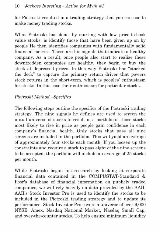
Piotroski Method –Specifics
The following steps outline the specifics of the Piotroski trading
strategy. The nine signals he defines are used to screen the
initial universe of stocks to result in a portfolio of those stocks
most likely to rise in price as people gain confidence in each
company’s financial health. Only stocks that pass all nine
screens are included in the portfolio. This will yield an average
of approximately four stocks each month. If you loosen up the
constraints and require a stock to pass eight of the nine screens
to be accepted, the portfolio will include an average of 25 stocks
per month.
While Piotroski began his research by looking at corporate
financial data contained in the COMPUSTAT-Standard &
Poor's database of financial information on publicly traded
companies, we will rely heavily on data provided by the AAII.
AAII's Stock Investor Pro is used to identify the stocks to be
included in the Piotroski trading strategy and to update its
performance. Stock Investor Pro covers a universe of over 9,000
NYSE, Amex, Nasdaq National Market, Nasdaq Small Cap,
and over-the-counter stocks. To help ensure minimum liquidity

Action – Myth #1 11
and financial reporting standards over-the-counter bulletin
board stocks and ADRs were excluded.
You can learn more about the American Association of
Individual Investors at www.aaii.com. The following
description of the Piotroski trading strategy is derived from the
description published by AAII. AAII runs the screens for the
end of each month and generally publishes the results in the
middle of the following month.
Piotroski first limited his universe to the bottom 20% of stocks
according to their price-to-book value ratio. Price-to-book value
was a favorite measure of value investors such as Benjamin
Graham and his disciples who sought companies with a share
price below their book value per share. In the short-run the
market can overreact to information and push prices away
from their true value. Because of this, measures such as price-
to-book-value ratio help to identify which stocks may be truly
undervalued.
Valuation levels of stocks vary over time, often dramatically
from bear market bottoms to bull market tops. During the
depths of a bear market, many firms can be found selling for a
price-to-book ratio less than one. In the latter stages of a bull
market, few companies other than troubled firms sell for less
than book value per share.
Piotroski found that most stocks trading with an extremely low
price-to-book-value were either neglected or financially
troubled firms. Small, thinly traded stocks are rarely followed
by analysts. The flow of information is limited for these stocks
and can lead to mispriced stocks. Analysts typically ignore
these stocks and tend to focus on stocks with general interest.
This points out another “feature” of the Piotroski trading
strategy. Most of the stocks selected by the initial price-to-book

12 Jackass Investing – Action for Myth #1
value screen are low capitalization stocks. This does not pose a
problem for most individuals, but may limit investment by the
larger mutual funds and hedge funds, as they may not be able
to invest large amounts in many of the selected stocks. As
described in Myth #15 – The Largest Investors Hold All the
Cards, this ability to buy and sell small capitalization stocks is
an investment advantage held by smaller individuals over
large institutional investors.
Once the price-to-book screen has identified the 20% of stocks
that are most undervalued, Piotroski’s 9-point ranking system
comes into play. Profitability, financial leverage, liquidity, and
operating efficiency are examined using popular ratios and
basic financial elements that are easy to use and interpret.
Stocks that pass all nine screens are included in the portfolio.
Minimum Profitability
Piotroski awarded up to four points for profitability: one for
positive return on assets, one for an improvement in return on
assets over the last year, one for positive cash flow from
operations, and one if cash flow from operations exceeds net
income. These are simple test that are easy to measure.
Because the requirements are minimal, there is no need to
worry about industry, market, or time specific comparisons.
1. Return on Assets. Piotroski defined return on assets
(ROA) as net income before extraordinary items for the
fiscal year preceding the analysis divided by total assets
at the beginning of the fiscal year. AAII’s Stock Investor
Pro deviates by using net income after extraordinary
items in its calculation. ROA examines the return
generated by the assets of the firm. Piotroski did not
look for high levels of ROA, only a positive figure. While
the screen may not seem to be very restrictive, he found
that over 40% of the low price-to-book-value stocks had
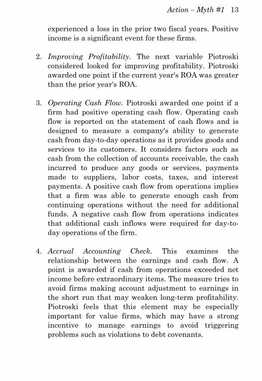
Action – Myth #1 13
experienced a loss in the prior two fiscal years. Positive
income is a significant event for these firms.
2. Improving Profitability. The next variable Piotroski
considered looked for improving profitability. Piotroski
awarded one point if the current year's ROA was greater
than the prior year's ROA.
3. Operating Cash Flow. Piotroski awarded one point if a
firm had positive operating cash flow. Operating cash
flow is reported on the statement of cash flows and is
designed to measure a company's ability to generate
cash from day-to-day operations as it provides goods and
services to its customers. It considers factors such as
cash from the collection of accounts receivable, the cash
incurred to produce any goods or services, payments
made to suppliers, labor costs, taxes, and interest
payments. A positive cash flow from operations implies
that a firm was able to generate enough cash from
continuing operations without the need for additional
funds. A negative cash flow from operations indicates
that additional cash inflows were required for day-to-
day operations of the firm.
4. Accrual Accounting Check. This examines the
relationship between the earnings and cash flow. A
point is awarded if cash from operations exceeded net
income before extraordinary items. The measure tries to
avoid firms making account adjustment to earnings in
the short run that may weaken long-term profitability.
Piotroski feels that this element may be especially
important for value firms, which may have a strong
incentive to manage earnings to avoid triggering
problems such as violations to debt covenants.

14 Jackass Investing – Action for Myth #1
In AAII’s Stock Investor Pro, Income after taxes
represents income before extraordinary items so the
screen looks for firms with cash from operations greater
than income after taxes for the most recent fiscal year.
5. Financial Leverage. Piotroski awards one point if a
company’s ratio of debt to total assets declined in the
past year, He defined debt to total assets as total long-
term debt plus the current portion of long-term debt
divided by average total assets. The higher the figure
the greater the financial risk. Judicious use of debt
allows a company to expand operations and leverage the
investment of shareholders provided that the firm can
earn a higher return than the cost of debt. Normally,
the more stable the cash flow of a firm, the greater
financial risk a company can assume. However, a
company must meet the rules (covenants) along with
the interest payments of its debt or risk bankruptcy and
complete loss of control of the firm. By raising
additional external capital, a financially distressed firm
is signaling that it is unable to generate sufficient
internal cash flow. An increase in long-term debt will
place additional constraints on the financial flexibility of
a firm, and will likely come at great cost.
6. Liquidity. To judge liquidity, a company earns one point
if its current ratio at the end of its most recent fiscal
year increased compared to the prior fiscal year.
Liquidity ratios examine how easily the firm could meet
its short-term obligations, while financial risk ratios
examine a company's ability to meet all liability
obligations and the impact of these liabilities on the
balance sheet structure.
The current ratio compares the level of the most liquid
assets (current assets) against that of the shortest

Action – Myth #1 15
maturity liabilities (current liabilities). It is computed
by dividing current assets by current liabilities. A high
current ratio indicates high level of liquidity and less
risk of financial trouble. Too high a ratio may point to
unnecessary investment in current assets or failure to
collect receivables or a bloated inventory, all negatively
affecting earnings. Too low a ratio implies illiquidity
and the potential for being unable to meet current
liabilities and random shocks that may temporarily
reduce the inflow of cash.
Piotroski assumed that an improvement in the current
ratio is good signal regarding a company's ability to
service its current debt obligations. He also indicated in
a footnote that the decline in current ratio was only
significant if the current ratio is near one.
7. Equity. The final capital structure element awards one
point if the firm did not issue common stock over the
last year. Similar in concept to an increase in long-term
debt, financially distressed companies that raise
external capital could be indicating that they are unable
to generate sufficient internal cash flow to meet their
obligations. Additionally, issuing stock while its stock
price is depressed (low price-to-book) highlights the
weak financial condition of the company.
We screen for stocks that have maintained or reduced
the number of outstanding shares during their last
fiscal year.
8. Gross Profit Margin. Companies gain one point for
showing an increase in their gross margin. Long-term
investors buy shares of a company with the expectation
that the company will produce a growing future stream
of cash. Profits point to the company's long-term growth

16 Jackass Investing – Action for Myth #1
and staying power. Gross profit margin reflects the
firm's basic pricing decisions and its material costs.
Computed by dividing gross income (sales minus cost of
goods sold) by sales for the same time period. The
greater the margin and the more stable the margin over
time, the greater the company's expected profitability.
Trends should be closely followed because they
generally signal changes in market competition.
Piotroski zeroed in on improving gross profit margin
because it serves as an immediate signal of an
improvement in production costs, inventory costs, or
increase in the sale's price of the company's product or
service.
9. Asset Turnover. The final element in Piotroski's
financial scoring system adds a point if asset turnover
for the latest fiscal year is greater than the prior year's
turnover.
Asset turnover (total sales divided by beginning period
total assets) measures how well the company's assets
have generated sales. Industries differ dramatically in
asset turnover, so comparison to firms in similar
industries is crucial. Too high a ratio relative to other
firms may indicate insufficient assets for future growth
and sales generation, while too low an asset turnover
figure points to redundant or low productivity assets.
An increase in the asset turnover signifies greater
productivity from the asset base and possibly greater
sales levels.

Action – Myth #1 17
Summary of the Stock Screens used in the Piotroski Trading
Strategy
At the start of each month run the following stock screens. The
stocks that make it through all of the screens constitute the
Piotroski portfolio for that month. Select stocks for which:
First, The price-to-book ratio ranks in the lowest 20% of the
entire AAII Stock Investor Pro database, then:
The return on assets for the last fiscal year (Y1) is
positive
Cash from operations for the last fiscal year (Y1) is
positive
The return on assets ratio for the last fiscal year (Y1) is
greater than the return on assets ratio for the fiscal
year two years ago (Y2)
Cash from operations for the last fiscal year (Y1) is
greater than income after taxes for the last fiscal year
(Y1)
The long-term debt to assets ratio for the last fiscal year
(Y1) is less than the long-term debt to assets ratio for
the fiscal year two years ago (Y2)
The current ratio for the last fiscal year (Y1) is greater
than the current ratio for the fiscal year two years ago
(Y2)
The average shares outstanding for the last fiscal year
(Y1) is less than or equal to the average number of
shares outstanding for the fiscal year two years ago (Y2)

18 Jackass Investing – Action for Myth #1
The gross margin for the last fiscal year (Y1) is greater
than the gross margin for the fiscal year two years ago
(Y2)
The asset turnover for the last fiscal year (Y1) is greater
than the asset turnover for the fiscal year two years ago
(Y2)
You can track the portfolio and performance of the Piotroski
trading strategy by becoming a member of AAII, which I highly
recommend, at www.AAII.com.

19
Action – Myth #3
In addition to providing you with a usable trading strategy,
this section shows how:
1. a hypothesis/concept (fading the sentiment of the most
aggressive retail investors) leads to
2. collection of the data relevant to identifying the
sentiment extremes, which leads to
3. a study that indicates the valid basis for a trading
strategy, that leads to
4. development of the actual trading strategy to exploit the
initial hypothesis
Once this process is understood, it can be expanded to produce
dozens of trading strategies that exploit numerous, unrelated
return drivers. This is the approach my firm, Brandywine
Asset Management, first developed almost 30 years ago and
continues to employ today.
The majority of people do not employ a systematic process
when they invest their money. As a result, they react
emotionally to every market move or geopolitical event. The
result, as shown in the DALBAR studies, is that they
dramatically underperform the average performances of the
mutual funds and ETFs in which they invest. This provides us
with a great opportunity to outperform those same funds.
Because the majority of people are so consistent at mis-timing
the market, we can use them as our George Costanza indicator
and do the opposite.
There are numerous measures of market sentiment. Some are
quite direct. Others esoteric. In 1996 my trading was
highlighted in an article in the financial weekly Barron’s after I
captured sizable profits from the grain market rally that

20 Jackass Investing – Action for Myth #3
spring. In the same article was the following comment
regarding the timing indicator used by another trader. “[Trader
name] has developed his own set of indicators such as the
number of dental operations performed on pets. They were up
100% last year, indicating a jump in the spending of disposable
income. Ergo, inflation.”
This trader clearly did not employ the K-I-S-S (Keep It Simple
Stupid) method! There were certainly more direct ways to
measure investor sentiment than dental operations performed
on pets. Unfortunately, a couple of years after this article was
published the trader lost substantial money in the Asian
markets, resulting in a total loss for him and the people who
entrusted their money to him.
I prefer to employ more direct measures of investor sentiment.
Some of these investor sentiment measures are based on direct
surveys of market participants. These include the surveys
conducted by Investors Intelligence (II) and the American
Association of Individual Investors (AAII). II surveys over one
hundred independent market newsletters and records each
advisor’s stance on the U.S. stock market as bullish, bearish or
correction. They have applied a consistent approach to their
record-keeping since they began the survey in 1963.
Interestingly, when the founder of Investors Intelligence, AW
Cohen, first developed the survey he expected that the best
time to be long the market would be when most advisors were
bullish. As we all know now, this proved to be exactly opposite
the truth. The majority of advisors are almost always wrong at
market turning points. The Investors Intelligence website is
located at: http://www.investorsintelligence.com/.
I already introduced you to the AAII. The AAII states that they
“arm individual investors with the education and tools they
need to build wealth.” One of the tools they provide is a weekly
measure of the percentage of individuals who are bullish,

Action – Myth #3 21
bearish or neutral on the stock market in the short-term. The
AAII also surveys people on the percentage of their assets they
have allocated to stocks, bonds and cash.
One of the more recent measures has been developed by
TrimTabs Investment Research. TrimTabs is an investment
research firm focused on equity market liquidity. They develop
quantitative trading models that incorporate supply and
demand factors, rather than the conventional price or earnings
data.
TrimTab’s research confirms what we learned in Myth #3,
people are poor market timers and in particular, people who
place money in leveraged stock market ETFs are “impressively
wrong in both directions.”
According to TrimTabs’ model (developed by Vincent Deluard),
in the week following inflows into leveraged U.S. equity ETFs,
the market falls by an annualized 13.7% and in the week
following outflows the market rises by an annualized 10.3%.
This creates an opportunity to develop a trading strategy based
specifically on the inability of people to successfully time the
market.
The Sentiment Strategy - Concept
Based on the TrimTabs study, I developed a sentiment-based
trading strategy that takes both long and short directional
positions in the U.S. stock market, depending on whether
people are aggressively selling or buying stocks (through
ETFs), respectively. In keeping with what we learned in Myth
#3, the strategy does the opposite of what most people are
doing. It buys the SPDR S&P 500 ETF (SPY) when people are
bearish and buys the ProShares Short S&P 500 ETF (SH)
(which attempts to produce the inverse of the S&P 500 index
each day) when people are bullish.

22 Jackass Investing – Action for Myth #3
The Sentiment Strategy - Performance
Because most inverse and leveraged ETFs began trading in the
mid 2000s, flows in these ETFs started being meaningful in
2006. Because (as you’ll see in the strategy specifics section)
the strategy requires one year of data before it can start
trading, I started the track record in January 2007. This gives
us four full years of performance data, including the financial
crisis. I did not include interest income for the 74% of the time
that the strategy is out of the market. Figure 3 and Figure 4
display the performance of the sentiment strategy compared
with a long position held in the S&P 500 Index.
The sentiment strategy beat the S&P 500 by about 95% in the
four years ending in 2010. What is more impressive is that the
sentiment strategy achieved this performance by being
invested only 26% of the time. In other words, the sentiment
strategy trades very little, but it trades very well. The
sentiment strategy achieved a positive rate of return in 75% of
the months. As you can see in the chart in Figure 4, the
sentiment strategy achieves most of its gains during sharp
market sell-offs - when investors are most emotional and more
prone to mistakes. As a result, the sentiment strategy is a
great edge against the passive long positions of your portfolio.
All you need to trade this strategy are the guts to go against
the crowds in times of intense market stress.

Action – Myth #3 23
Performance of the Sentiment Strategy
Relative to SPY (Spiders)
Performance of the Sentiment Strategy Relative to SPY (Spiders)
SPY SENTIMENT
(SPIDERS) STRATEGY
YEARS 4.0 4.0
AVERAGE ANNUAL RETURN -0.96% 17.11%
ANNUALIZED VOLATILITY 19.60% 17.52%
MAXIMUM DRAWDOWN -55.19% -10.82%
% PROFITABLE MONTHS 56% 75%
% PROFITABLE ROLLING 12 MONTHS 43% 100%
% PROFITABLE YEARS 75% 100%
TIME IN MARKET 100.00% 26.22%
Figure 3
Figure 4

24 Jackass Investing – Action for Myth #3
Sentiment Strategy ETF Listing
Figure 5
Action – Myth #3 25
Sentiment Strategy – Specifics:
Here are the specific trading rules of the strategy:
1. Determine level of bullishness or bearishness of
investors in leveraged ETFs.
Figure 5 shows the current ETF Listing for the
Sentiment Strategy.
Bloomberg and other data providers report ETF share
data on a daily basis. For Bloomberg users, just type:
FASSO Index HP <Enter> to access the historical
shares outstanding of FAS (Direxion Financial Bull 3X).
Yahoo! Finance also reports the latest available data by
ticker.
Flow is measured as change in shares multiplied by
price. Of course, flows need to be adjusted by the
leverage used in the ETF. For example, inflows and
outflows to/from an ETF that attempts to return two
times the daily return of the S&P 500 (such as the
ProShares Ultra S&P 500 ETF or “SSO”) will get two
times the weighting of those that flow into or out of a
single leveraged ETF (such as SPY). Inflows into inverse
ETFs are counted as outflows (from stocks). The
resultant total we will call the “Daily Money Flow”
(DMF).
2. Each day calculate the average of the past ten (10) days
DMF. This is the “10dDMF.” Convert the 10dDMF into
a normalized score using its rolling 100-day mean and
standard deviation. Normalized score is calculated by
subtracting the mean from an observation and dividing

26 Jackass Investing – Action for Myth #3
the result by the historical standard deviation. A
normalized score of 2.0 would imply that flows are two
standard deviations greater than the historical mean
(note that for normally distributed variables, such
occurrences happen about 2.5% of the time).
If the normalized score of 10dDMF is below -1.75 (which
indicates very negative sentiment), buy SPY. If the
normalized score of 10dDMF is above 1.75 (which
indicates ebullient sentiment), buy SH (ProShares Short
S&P 500)
3. Hold the position for 5 days. If the buying/selling
criteria remain in effect, the 5-day hold period resets
with each day the normalized score exceeds the
threshold. Also, if the normalized score falls within the
threshold and then exceeds the threshold again during
the hold period, a new entry signal is issued, and the 5-
day hold period begins again.
Note 3-1: Results shown in this Action Section are slightly
different than the results shown in the book due to
adjustments in the strategy algorithm and the ETF list.
Note 3-2: Transaction costs are assumed to be 0.10% per
transaction.

27
Action – Myth #4
In Myth #4 I discussed that fact that the major stock market
indexes were not created with the goal of maximizing returns,
but with the goal of being representative. In addition, they
allocate to their constituent stocks in a way that creates quirky
biases in their portfolios. Because of this there are better
alternatives for you to get broad stock market exposure than to
place your money into the most popular stock index funds, such
as those that track the S&P 500 Index. Prior to 2005 your only
option would have been to create your own “actively passive”
index fund, a significant undertaking. But today you can put
money into one of the many new index funds that have been
created with the intent of “performing,” rather than simply
being “representative.”
Index Innovation
There have been numerous studies conducted that show that
by focusing on some basic attributes; certain stocks may
outperform others over time. For example, in Myth #1 we saw
that the primary driver of stock returns long-term was
corporate earnings growth. And in Myth #4 I referenced a
study that established that higher dividend payout ratios (the
percentage of a company’s earnings that are paid to
shareholders as dividends) leads to higher earnings growth.
While you can develop your own stock selection methods to
attempt to identify such stocks for inclusion in your portfolio,
only the largest accounts will be able to diversify across the
hundreds of stocks necessary to obtain true index-like
diversification. Fortunately others have done this for us. Since
2005, many new indexes have been created with the goal of
systematically maximizing returns by following a clearly-
defined set of rules, while still following a (reasonably) low-
turnover approach. We now have a selection of “performance”
(my term) index funds based on these new indexes that can
28 Jackass Investing – Action for Myth #4
serve as an alternative to the “representative” index funds such
as those based on the S&P 500.
Performance index funds can be classified into three primary
categories. These are Equal-Weighted, Fundamental and
Efficient. Equal-Weighted indexes are described by their
classification. The stocks in these indexes are held in equal
allocations, so that a 1% move in any stock has the same
impact on the index as a 1% move in any of the other stocks.
Fundamental indexes allocate to each stock in the index based
on factors such as each company’s earnings, dividend growth,
positive changes in analyst recommendations, buying of shares
by company insiders or book value. Efficient indexes weight
each stock in the index based on quantitative information such
as expected returns, correlations and volatilities.
The major index providers, such as S&P and FTSE, have
jumped on the Performance index bandwagon. In 2002 S&P
launched an equal-weighted version of its S&P 500 Index. In
2005 FTSE teamed with Research Affiliates LLC to create a
series of fundamental indexes and later with EDHEC to create
a series of efficient indexes. As the FTSE EDHEC indexes were
only developed in 2010, there are not yet any ETFs trading
pursuant to their methodologies. However, there are a number
of ETFs trading pursuant to equal-weighted and fundamental
indexes. The equal-weighted indexes are based on the
traditional Representative indexes such as the S&P 500 and
the Russell indexes. They allocate to the same stocks as those
in the indexes but on an equal-weighted basis. The
fundamental indexes may start out by looking at the stocks
that make up one of the Representative indexes, but they
ultimately select only the subset of those stocks that exhibit
the characteristics that have been found to be predictive of
future share price appreciation.
Action – Myth #4 29
In this Action I present the performance of four Performance
ETFs; one that is equal-weighted, the Rydex S&P 500 Equal
Weight ETF (RSP); and three based on fundamental indexes;
the PowerShares FTSE RAFI U.S. 1000 ETF (PRF), the
Vanguard Dividend Appreciation ETF (VIG), and the
Guggenheim Insider ETF (NFO). These funds can serve as
replacements for the typical index fund(s) that people
incorporate in their portfolios.
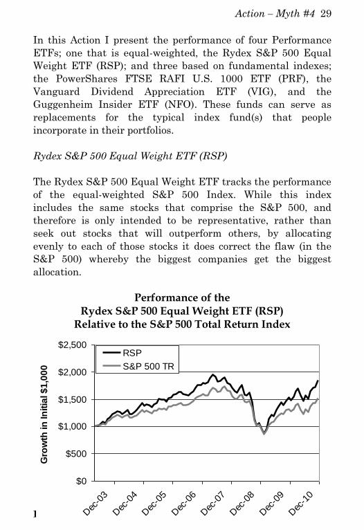
Rydex S&P 500 Equal Weight ETF (RSP)
The Rydex S&P 500 Equal Weight ETF tracks the performance
of the equal-weighted S&P 500 Index. While this index
includes the same stocks that comprise the S&P 500, and
therefore is only intended to be representative, rather than
seek out stocks that will outperform others, by allocating
evenly to each of those stocks it does correct the flaw (in the
S&P 500) whereby the biggest companies get the biggest
allocation.
Performance of the Rydex S&P 500 Equal Weight ETF (RSP)
Relative to the S&P 500 Total Return Index
Figure 6
$0
$500
$1,000
$1,500
$2,000
$2,500
Dec
-10
Dec
-09
Dec
-08
Dec
-07
Dec
-06
Dec
-05
Dec
-04
Dec
-03
Gro
wth
in
In
itia
l $
1,0
00
RSP
S&P 500 TR
30 Jackass Investing – Action for Myth #4
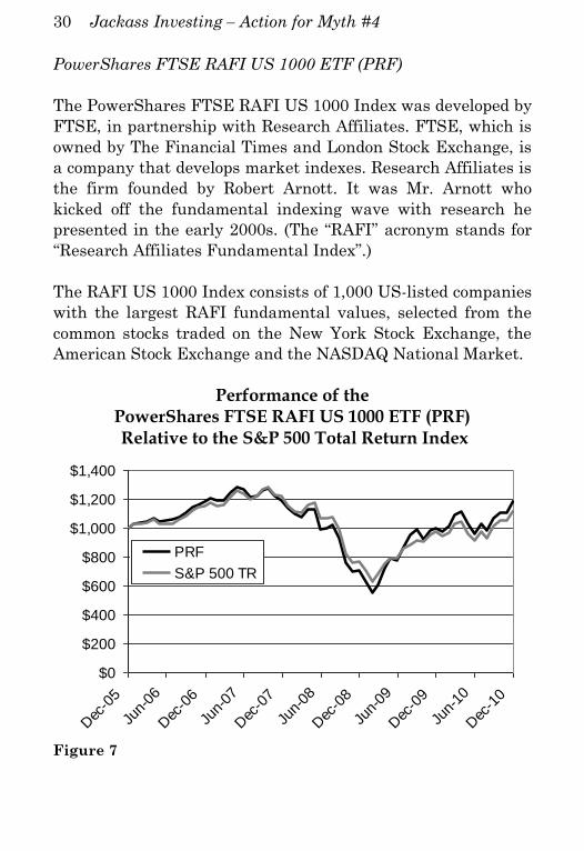
PowerShares FTSE RAFI US 1000 ETF (PRF)
The PowerShares FTSE RAFI US 1000 Index was developed by
FTSE, in partnership with Research Affiliates. FTSE, which is
owned by The Financial Times and London Stock Exchange, is
a company that develops market indexes. Research Affiliates is
the firm founded by Robert Arnott. It was Mr. Arnott who
kicked off the fundamental indexing wave with research he
presented in the early 2000s. (The “RAFI” acronym stands for
“Research Affiliates Fundamental Index”.)
The RAFI US 1000 Index consists of 1,000 US-listed companies
with the largest RAFI fundamental values, selected from the
common stocks traded on the New York Stock Exchange, the
American Stock Exchange and the NASDAQ National Market.
Performance of the PowerShares FTSE RAFI US 1000 ETF (PRF) Relative to the S&P 500 Total Return Index
Figure 7
$0
$200
$400
$600
$800
$1,000
$1,200
$1,400
Dec
-05
Jun-
06
Dec
-06
Jun-
07
Dec
-07
Jun-
08
Dec
-08
Jun-
09
Dec
-09
Jun-
10
Dec
-10
PRF
S&P 500 TR

Action – Myth #4 31
Vanguard Dividend Appreciation ETF (VIG)
This Vanguard ETF is managed by Vanguard and tracks the
Mergent Dividend Achievers Index. The Mergent Dividend
Achievers Index follows U.S. listed companies that have
consistently increased their annual regular dividends for at
least the past ten consecutive years and have met certain
liquidity screens. (Mergent is a provider of financial data that
also develops and licenses equity and fixed income indexes
based on its proprietary investment methodologies.)
Performance of the Vanguard Dividend Appreciation ETF (VIG) Relative to the S&P 500 Total Return Index
Figure 8
$0
$200
$400
$600
$800
$1,000
$1,200
$1,400
Dec
-10
Jun-
10
Dec
-09
Jun-
09
Dec
-08
Jun-
08
Dec
-07
Jun-
07
Dec
-06
Jun-
06
VIG
S&P 500 TR

32 Jackass Investing – Action for Myth #4
Guggenheim Insider ETF (NFO)
The Guggenheim Insider ETF tracks the performance of the
Sabrient Insider Sentiment Index.1 This is an index of
approximately 100 stocks that are selected (out of
approximately 6,000 eligible securities) to be purchased
because company insiders have been active buyers of the stock
and earnings expectations have increased. Stocks selected
pursuant to these factors have shown to produce above-average
returns in more than a decade of back-testing. Although there
are other funds based on fundamental factors that could also be
selected to serve as Performance indexes in your portfolio, I am
presenting NFO for two primary reasons. First, I believe in the
power of legal “insider information” as a predictor of a stock’s
price, and second, the fund now has more than four years of
actual in-market performance. Many of the other
fundamentally-based ETFs are more recently formed.
Performance of the Guggenheim Insider ETF (NFO)
Relative to the S&P 500 Total Return Index
Figure 9
$0
$200
$400
$600
$800
$1,000
$1,200
$1,400
$1,600
Dec-
10
Dec-
09
Dec-
08
Dec-
07
Dec-
06
NFO
S&P 500 TR

Action – Myth #4 33
1Joshua Anderson, “The Sabrient Insider Sentiment Index,”
Sabrient (October 20, 2006).
34
Action – Myth #6
Buy low, sell high is a great concept that fails in its
implementation. As I showed in both Myth #6 – Buy Low, Sell
High and Myth #7 – It’s Bad to Chase Performance, the
opposite approach is what actually works.
One such “opposite” stock trading strategy was developed by
William O’Neil, the founder of Investor’s Business Daily. Mr.
O’Neil developed his strategy by looking at the characteristics
exhibited by the best performing stocks prior to them posting
their large gains. He identified seven key indicators for
inclusion in this trading strategy. These indicators form the
mnemonic – CAN SLIM – that spells out the name of the
trading strategy. Because this trading strategy generally
produces portfolios that contain less than 10 stocks, it is
suitable for small portfolios.
The CAN SLIM concepts were first published by Mr. O’Neil in
1988 in the first edition of his best-selling book, How to Make
Money in Stocks. The book is now in its fourth printing. (See:
O’Neil, William J. "How to make Money in Stocks: A Winning
System in Good Times or Bad." 1988.) The AAII developed and
tracks a version of the CAN SLIM strategy and ranks it among
the leading stock trading strategies over the past ten years.
Over their entire test period, from January 1998 through
December 2010, the CAN SLIM trading strategy produced a
23% average annualized return. I have adjusted the returns to
include a cost of 4% each year to account for the transaction
costs that could have been incurred in actual trading. Figure 10
and Figure 11 present this performance.
Note 6-1: As of January 2011, transaction costs are assumed to
be 0.50% per transaction.

Action – Myth #6 35
Growth in $1,000 Allocated to CAN SLIM Trading Strategy
on January 1, 1998
CAN SLIM Trading Strategy Annual Returns
The CAN SLIM Strategy
The AAII has developed a systematic process for trading CAN
SLIM based on their interpretation of the strategy as described
by William O’Neil. The following description, which details the
criteria underlying each letter in the CAN SLIM mnemonic, is
derived from this interpretation. A description of each letter in
Figure 10. Source: AAII.com
Figure 11. Source AAII.com
$0
$2,000
$4,000
$6,000
$8,000
$10,000
$12,000
$14,000
$16,000
$18,000
$20,000
Dec
-97
Dec
-98
Dec
-99
Dec
-00
Dec
-01
Dec
-02
Dec
-03
Dec
-04
Dec
-05
Dec
-06
Dec
-07
Dec
-08
Dec
-09
Dec
-10
1998 23.15% 2005 19.28%
1999 31.23% 2006 24.53%
2000 32.73% 2007 25.50%
2001 48.74% 2008 -14.07%
2002 15.80% 2009 89.81%
2003 72.29% 2010 -27.31%
2004 -7.64%

36 Jackass Investing – Action for Myth #6
the acronym is followed at the end of this Action by a list of the
specific criteria underlying the AAII interpretation of the CAN
SLIM trading strategy.
C = Current Quarterly Earnings per Share: How Much Is
Enough?
The CAN SLIM approach focuses on companies with proven
records of earnings growth but that are still in a stage of
earnings acceleration. O'Neil's study of winning stocks
highlights the strong quarterly earnings per share of the
securities prior to their significant price run-ups.
When screening for quarterly earning increases, it is
important to compare a quarter to its equivalent quarter
last year – i.e., this year's second quarter compared to last
year's second quarter. Many firms have seasonal earnings
patterns and comparing similar quarters eliminates any
bias arising from this seasonality.
O'Neil recommends looking for stocks with a minimum
increase in quarterly earnings of 18% to 20% over the same
quarterly period one year ago. When examining a
percentage change it is not only important to check the
figures for unusually small base numbers that may distort
the percentage change figures, but it is also important to
check if any of the numbers in the calculation are negative.
A change in sign, as in a negative to a positive, requires
special consideration and may result in misleading
screening results. When screening on user-defined fields
such as custom growth rates, you may find it useful to
include some secondary or qualifying criterion to help
ensure proper screening results. In the CAN SLIM screen,
positive earnings for the current quarter are required to
help make the results of the growth rate calculation more
meaningful.

Action – Myth #6 37
Whenever you are working with earnings, the issue of how
to handle extraordinary earnings comes into play. One-time
events can distort the actual trend in earnings and make
company performance look better or worse than a
comparison against a firm without special events. O'Neil
recommends excluding these non-recurring items from the
analysis. The AAII screen examines growth in earnings
from continuing operations only.
So the first two screening filters that make up the trading
strategy are:
a. quarterly growth rate greater than or equal to
20%; and
b. positive earnings per share from continuing
operations for the current quarter.
A = Annual Earnings Increases: Look for Meaningful
Growth
Beyond looking for strong quarterly growth, O'Neil likes to
see an increasing rate of growth. An increasing growth rate
in quarterly earnings per share is so important in the CAN
SLIM system that O'Neil warns shareholders to consider
selling holdings of those companies that show a slowing
rate of growth two quarters in row. This screen specifies
that the growth rate from the quarter one year ago to the
latest quarter be higher than the previous quarter's
increase from its counterpart one year prior. Basically, the
current quarter's growth over the past 12-month period
must be better than the previous quarter's growth over the
past 12-month period.
In addition, the winning stocks in O'Neil's study had a
steady and significant record of annual earnings in addition

38 Jackass Investing – Action for Myth #6
to a strong record of current earnings. The CAN SLIM
system tries to identify the strong companies leading the
current market cycle.
The primary screen for annual earning increases that
O'Neil uses is increasing earnings per share in each of the
last five years. In applying this screen, we specify that
earnings per share from continuing operations be higher for
each year when compared against the previous year. To
help guard against any recent reversal in trend, a criterion
is included requiring that the earnings over the last 12
months be greater than or equal to earnings from the latest
fiscal year. This group of criteria proved to be the most
stringent independent filter.
O'Neil also recommends screening for companies showing a
strong annual growth rate of 25% or 50% over the last five
years. The winning companies in O'Neil's study had a
median growth rate of 21%. O'Neil specifies a minimum
annual growth rate of 25% in earnings per share from
continuing operations over the last five years. This criterion
proved to be the second most restrictive screen when used
independently.
N = New Products, New Management, New Highs: Buying
at the Right Time
O'Neil feels that a stock needs a catalyst to start a strong
price advance. In his study of winning stocks, he found that
95% of the winning stocks had some sort of fundamental
spark to push the company ahead of the pack. This catalyst
can be a new product or service, a new management team
after a period of lackluster performance or even a structural
change in a company's industry, such as a new technology.
Action – Myth #6 39
These are very few qualitative factors that lend themselves
to inclusion in a fully systematic trading strategy. However,
the existence of a catalyst is often reflected as a jump in the
stock price. O’Neill recognizes this as well and emphasizes
that investors should pursue stocks showing strong upward
price movements. O'Neil says that stocks that seem too
high-priced and risky most often go even higher, while
stocks that seem cheap often go even lower. (I agree. In
Myth #7 – It’s Bad to Chase Performance” I discuss the
existence and cause of market trends and in the next Action
present a trading strategy that you can use to profit from
them.)
O'Neil's newspaper, Investor's Business Daily, highlights
stocks within 10% of their 52-week high and this is the
criterion AAII established for their screen. Used
independently the screen allows about one-third of the
companies to pass the filter. The number of companies
passing will vary over the course of the market cycle. One
would expect many companies to pass during a strong
market expansion, while a smaller number of companies
would pass during the early stage of a bear market.
S = Supply and Demand: Small Capitalization Plus Volume
Demand
As the catalyst starts pushing the price of a company's
stock up, those firms with a smaller number of shares
outstanding should increase more quickly than those with a
large number of outstanding shares. In his study of winning
stocks, O'Neil found that 95% of the winning stocks had
fewer than 25 million shares outstanding, while the median
for the group was 4.6 million.
In a separate study of stock market winners by Marc
Reinganum, published in the September 1989 issue of the
40 Jackass Investing – Action for Myth #6
AAII Journal, the findings resulted in a similar conclusion
and established the cut-off at 20 million outstanding
shares. The Reinganum study examined the characteristics
of stocks prior to their big price increase and found that the
median figure of the stocks in the study was 5.7 million
shares, which doubled during the two years that each
winning stock was examined. This probably indicates that
firms split their shares during their big price increase.
What this also indicates is that the CAN SLIM trading
strategy lets smaller investors take advantage of their size.
Because of the small size of the companies selected by the
CAN SLIM trading strategy, the largest mutual funds are
effectively unable to trade in these stocks.
O'Neil also feels that share buybacks, which reduce the
public float of company's stock, is positive because it
reduces the supply of the company's stock while boosting
per share earnings.
O'Neil suggests that investors consider looking at the actual
"float" of the stock. The float is the number of shares in the
hands of the public – determined by subtracting the
number of shares held by management from the number of
shares outstanding. Thus AAII requires a stock to have
fewer than 20 million shares available through the float in
order to be considered. When examined independently, this
criterion proves to be the least restrictive screen.
L = Leader or Laggard: Which is Your Stock?
O'Neil is not like the patient value investor – looking for
out-of-favor companies and willing to wait for the market to
come around to his viewpoint. Rather, he prefers to scan for
rapidly growing companies that are market leaders in
rapidly expanding industries. O'Neil advocates buying
among the best two or three stocks in a group. You should

Action – Myth #6 41
be compensated for any premium you pay for these leaders
with significantly higher rates of return.
After identifying a strong industry, O'Neil warns against
avoiding the market leaders by purchasing "sympathy"
stocks that are similar but significantly cheaper when
examined by factors such as price-earnings ratios and
weaker price performance. These stocks often continue to
languish while the market leaders continue their strong
rise.
O'Neil suggests using relative strength to identify market
leaders. Relative strength compares the performance of a
stock relative to the market as a whole. Relative strength is
typically reported with a base level of zero or one – in which
case the base level represents stock performance equal to
the market index. Numbers above the base level reflect
performance above the market index, while below-market
performance can be seen with figures below the base. AAII
uses a base level of zero.
Companies are often ranked by their relative strength
performance and their percentage ranking among all stocks
is calculated to show the relative position against other
securities. Investor's Business Daily presents the
percentage ranking of stocks and O'Neil recommends only
looking for stocks with a percentage rank of 70% or better –
stocks that have performed better than 70% of all stocks.
AAII requires the 52-week relative strength to equal or
exceed 70%.
I = Institutional Sponsorship: A Little Goes a Long Way
O'Neil warns against selecting low-priced stocks with small
capitalization and no institutional ownership, because these

42 Jackass Investing – Action for Myth #6
stocks have poor liquidity and often carry a lower-grade
rating.
O'Neil feels that a stock needs a few institutional sponsors
for it to show above-market performance. Three to 10
institutional owners are suggested as a reasonable
minimum number. This number refers to actual
institutional owners of the common stock, not institutional
analysts tracking and providing earnings estimates on
stocks.
Beyond looking for a minimum number of institutional
owners, O'Neil suggests that investors look at the past
record of the institutions. The analysis of the holdings of
successful mutual funds represents a good resource for the
investor because of the widely distributed information on
mutual funds.
AAII established a screen for stocks to have at least five
institutional owners.
It is difficult to strike a balance between looking for stocks
with room to expand further and stocks that may be over-
owned. O'Neil warns that while some institutional
sponsorship is required, once everyone has jumped on the
stock it may be too late to buy into it.
M = Market Direction: How to Determine It?
The final aspect of the CAN SLIM system looks at the
overall market direction. While it does not impact the
selection of specific stocks and is not included in the version
of the CAN SLIM strategy I present here, the trend of the
overall stock market has a tremendous impact on the
performance of the individual stocks you select. O'Neil
focuses on technical measures when determining the
Action – Myth #6 43
overall direction of the marketplace and recommends that
you sell 25% of your stocks when the market peaks and
begins a major reversal.
Summary of the stock screens used in the CAN SLIM Trading
Strategy
At the start of each month run the following stock screens. The
stocks that make it through all of the screens constitute the
CAN SLIM portfolio for that month. Select stocks for which:
The growth of earnings per share from continuing
operations, as of the latest fiscal quarter (Q1) over the
same quarter one year prior (Q5), is greater than or
equal to 20%
The growth of earnings per share from continuing
operations, as of the latest fiscal quarter (Q1) over the
same quarter one year prior (Q5) is greater than the
growth of earnings per share from continuing
operations, as of the previous fiscal quarter (Q2) over
the same quarter one year prior (Q6)
Earnings per share from continuing operations for the
two most recent fiscal quarters (Q1 and Q2) is positive
Growth in earnings per share from continuing
operations over the last five years is 25% or more
Earnings per share from continuing operations has
increased over each of the last five fiscal years as well as
over the last 12 months
The current stock price is within 10% of its 52-week
high

44 Jackass Investing – Action for Myth #6
The stock's float is less than 20 million shares
The 52-week relative strength is in the top 30% of the
entire database (percent rank greater than 70)
There are at least five institutional shareholders
You can track the portfolio and performance of the CAN SLIM
trading strategy by becoming a member of the AAII, which I
highly recommend, at www.AAII.com.

45
Action – Myth #7
In Myth #7 we saw that buying-and-holding the S&P
Diversified Trends Indicator outperformed, on a risk-adjusted
basis, a buy-and-hold position in the S&P 500 TR Index. The
reason for this is two-fold. One, the S&P DTI, despite trading
in just 24 markets, is more diversified than the S&P 500 TR,
which trades in 500. That is because the markets in the S&P
DTI include interest rate markets, currencies, precious metals,
grains, livestock and other commodities. They are not all
subject to the same event risk and therefore their prices move
more independent of each other than do the 500 stocks in the
S&P 500 TR. Two, the S&P DTI is adaptive. It follows trends.
When the trend in any given market is up it is long. When the
trend is down it is short. The S&P 500 TR in contrast, naively
holds on to long positions even when the trend is clearly down.
As good as the S&P DTI is however, it does have its flaws, as
were discussed in the myth. The primary flaw is that it applies
different rules to the energy markets than it does to other
markets. This appears to be a case of “curve-fitting” the
strategy to the observed results. But there’s an easy solution to
that problem. Simply apply the strategy consistently to all
markets.
In this Action I will present what is perhaps the simplest
possible trend following strategy, even simpler than underlying
the S&P DTI. We will apply this strategy equally to all markets
in the portfolio. Because this trading strategy is applied across
30 futures markets it requires $1 million for full diversification
and is therefore suitable only for the largest accounts. Small
accounts can however, invest in the mutual funds and ETFs
presented in the Action Section for Myth #20.

46 Jackass Investing – Action for Myth #7
The “Month-end Trend Strategy”
The name of this trading strategy describes its main
characteristic: it takes long and short positions in each market
in its portfolio based on the direction of the trend indicated by
the month-end closing price of each market. Specifically, there
are two components of the ETM Diversified Trend Strategy:
1. the specifics of the trend following system to be
employed
2. the selection of, and allocation among, the markets to be
included in the portfolio
Specifics of the Trend Following System
The trend following system underlying the Month-end Trend
Strategy incorporates one of the simplest possible algorithms,
yet it is effective in capturing longer-term trends. The system
will always be long or short in each market. Here’s how it
works: At month-end we will compare the price of each market
to that market’s 250-day moving average. A moving average is
simply the average of the closing prices of that market over the
250 trading days ending at month-end. If the market price at
month-end is below the moving average we will either
maintain our short position (if already short) or reverse our
long position to a short position in that market at the close of
trading on the first trading day of the following month. If the
market price at month-end is above the 250-day moving
average we will place an order (if not already long) to go long
that market at the close of trading on the first trading day of
the following month. We apply this system to a portfolio of 30
futures markets diversified across stock indexes, interest rate
contracts, currencies, energy, metals and agricultural markets.

Action – Myth #7 47
Market Selection and Allocation
It is important to avoid the market selection bias exemplified
by the inconsistent trading of energy markets in the S&P
Diversified Trends Indicator. To maintain consistency, the
Month-end Trend Strategy will trade a diversified portfolio of
futures markets that bases its market allocations simply on the
goal of producing consistent returns across a range of market
conditions. As a result, we allocate to each market with the
intent of creating a portfolio that is balanced across all
markets, so that no single market will, over time, dominate
performance. The following markets displayed in Figure 12
have been selected to provide broad portfolio diversification:
The allocation to each market is designed to ensure that over
time, each market will have a balanced impact on the volatility
of the entire portfolio. To achieve this we allocate to each
market based on the standard deviation of the daily move in
the price of each market over the prior 250 days. For example,
if over the past 250 trading days the Euro futures contract has
Figure 12
Commodities
Currencies
Metals
Energy
Stock
IndexesInterest
Rates
U.S. 30-yr. Bond
German Bund
Long Gilt (UK)
Japanese Government Bond
Eurodollar
S&P 500
DAX 30 (Germany)
FTSE 100 (UK)
Volatility index
Crude oil
Heating Oil
RBOB Gasoline
Natural Gas
Gold
Silver
Copper
Corn Sugar
Wheat Orange Juice
Soybeans Cotton
Coffee Live Cattle
Cocoa Lean Hogs
Euro
British Pound
Japanese Yen
Aussie Dollar

48 Jackass Investing – Action for Myth #7
averaged a move of $800 from one day to the next and corn has
averaged $400, then we will trade one Euro for every two corn
contracts. That gives us the relative allocation among all
markets. Now we need to calculate the specific number of
contracts to be traded in each market. This is a function of the
amount of portfolio volatility we are willing to accept. As a
rough rule of thumb, a million dollar account trading a total of
50 contracts across all markets will produce an average annual
standard deviation of returns approximately equal to that of
the S&P 500. For the purpose of calculating the performance
displayed in Figure 13 and Figure 14, I targeted a return over
the 20 year period 1991 – 2010 that was equal to the return
earned by the S&P 500 during that period. Because the Month-
end Trend Strategy is more diversified than the S&P 500 the
back-tests show it can achieve the same annualized return of
the S&P 500 but with only 52% of the S&P 500s annualized
volatility. The diversification benefit has an even greater
impact on the maximum drawdown. While the S&P 500 lost
more than 50% of its value during the financial crisis, the Trend
Strategy (which profited during the financial crisis) suffered a
maximum drawdown over its entire 20 year history of less than
12%, while targeting the same annualized return as the S&P 500.
This is the same trend following strategy that produced the
results displayed in Figure 36 in Myth #12. While that
performance, trading just five stock index futures contracts,
outperformed the S&P 500 on a risk-adjusted basis (the return
matched that of the S&P 500 Total Return Index while the
maximum drawdown was 47% less), risk is reduced even more
when the strategy is employed across 30 markets rather than
just five.
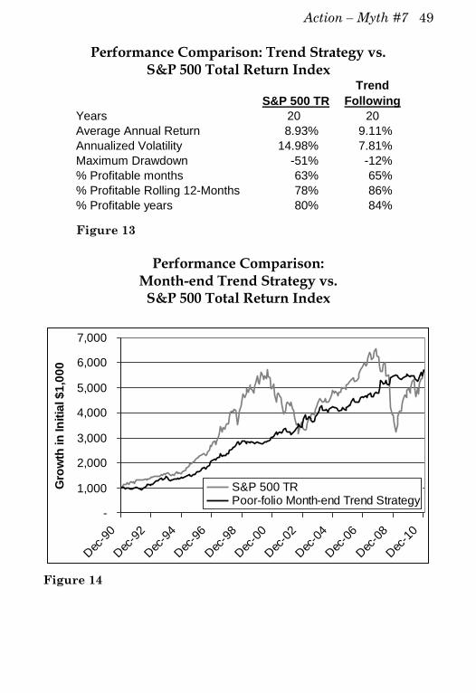
This simple trend-following strategy produced the following
back-tested returns relative to the S&P 500 Total Return Index
over the past 20 years.
Action – Myth #7 49
Performance Comparison: Trend Strategy vs. S&P 500 Total Return Index
Figure 13
Performance Comparison: Month-end Trend Strategy vs.
S&P 500 Total Return Index
Trend
Following
Years 20 20
Average Annual Return 8.93% 9.11%
Annualized Volatility 14.98% 7.81%
Maximum Drawdown -51% -12%
% Profitable months 63% 65%
% Profitable Rolling 12-Months 78% 86%
% Profitable years 80% 84%
S&P 500 TR
-
1,000
2,000
3,000
4,000
5,000
6,000
7,000
Dec
-90
Dec
-92
Dec
-94
Dec
-96
Dec
-98
Dec
-00
Dec
-02
Dec
-04
Dec
-06
Dec
-08
Dec
-10
Gro
wth
in
In
itia
l $
1,0
00
S&P 500 TRPoor-folio Month-end Trend Strategy
Figure 14

50
Action – Myth #8
In Myth #8 I showed that simply buying-and-holding stocks in
multiple industry sectors provided very little diversification
value, especially in bear markets, as the sector performances
are highly correlated with each other. But they are not
perfectly correlated and this opens up the opportunity to trade
pursuant to a disciplined strategy that attempts to identify and
allocate to the strongest sectors and avoid the weakest.
Schreiner Capital Management (SCM) is a registered
investment advisor that provides investors with active
management solutions. They have been trading client assets
pursuant to sector allocation strategies since 1989. The
strategy and performance presented here is an original sector
allocation strategy developed by SCM and differs from the
specific strategy they currently employ for their clients. Before
I present the strategy rules, let’s take a look at the
performance of the strategy relative to that of the S&P 500
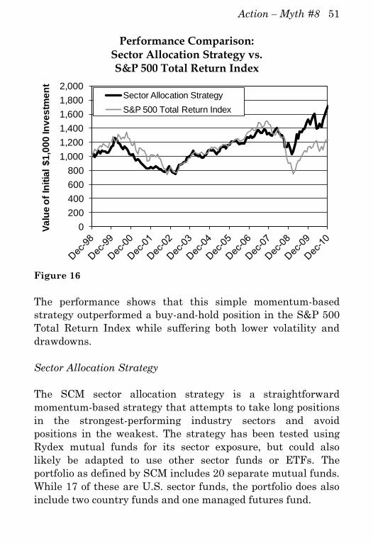
Total Return Index (Figure 15 and Figure 16).
Performance Comparison: Sector Allocation Strategy vs. S&P 500 Total Return Index
Figure 15
S&P 500 Total
Return
Sector Allocation Strategy
Years 12 12 Average Annual Return 0.21% 4.60% Annualized Volatility 16.12% 13.35% Maximum Drawdown -51% -41% % Profitable Months 56% 56% % Profitable Rolling 12-Mos. 61% 68% % Profitable Years 67% 67%
Action – Myth #8 51
Performance Comparison: Sector Allocation Strategy vs. S&P 500 Total Return Index
Figure 16
The performance shows that this simple momentum-based
strategy outperformed a buy-and-hold position in the S&P 500
Total Return Index while suffering both lower volatility and
drawdowns.
Sector Allocation Strategy
The SCM sector allocation strategy is a straightforward
momentum-based strategy that attempts to take long positions
in the strongest-performing industry sectors and avoid
positions in the weakest. The strategy has been tested using
Rydex mutual funds for its sector exposure, but could also
likely be adapted to use other sector funds or ETFs. The
portfolio as defined by SCM includes 20 separate mutual funds.
While 17 of these are U.S. sector funds, the portfolio does also
include two country funds and one managed futures fund.
0
200
400
600
800
1,000
1,200
1,400
1,600
1,800
2,000
Va
lue
of
Init
ial
$1
,00
0 In
ve
stm
en
t
Sector Allocation Strategy
S&P 500 Total Return Index

52 Jackass Investing – Action for Myth #8
These 20 Rydex mutual funds are:
Symbol Name Symbol Name
RYBIX Basic Materials RYOIX Biotechnology
RYCIX Consumer Products RYPIX Transportation
RYEIX Energy RYRIX Retailing
RYFIX Financial Services RYSIX Electronics
RYHIX Health Care RYTIX Technology
RYHRX Real Estate RYUIX Utilities
RYIIX Internet RYVIX Energy Services
RYKIX Banking RYEUX Europe 1.25x Strategy
RYLIX Leisure RYJHX Japan 2x Strategy
RYMIX Telecommunications RYMBX Commodities Strategy
Figure 17
The basic underlying rule is to buy each mutual fund, selected
from the list, when it shows a positive rate of change (ROC) in
price over the prior 42 trading days. Each fund gets a 5%
allocation of the cash allocated to this strategy. Once a position
is entered into, it is held in the strategy for a minimum of 21
trading days. Following 21 trading days, a position will then
exit if and when the ROC is negative.
Note 8-1: The strategy algorithm was adjusted for results
beginning January 2011, so results in the book may differ
slightly from the results included in the Performance Reports
on the interactive website.
Note 8-2: As of January 2011, transaction costs are assumed to
be 0.10% per transaction.
53
Action – Myth #10
As I showed in Myth #10, the ability of investors to be able to
sell stocks short provides value to the overall financial
markets. But short-selling also provides tremendous
opportunities to the short-sellers as well. First, holding short
positions in a stock portfolio can serve as a “hedge” to reduce
portfolio losses when there are sizable market sell-offs. But
short positions can also serve as a source of additional returns.
By selecting stocks of poorly run companies to sell short, the
short-seller will profit as other investors begin to recognize the
underperformance of those companies as well and sell the
stock. This collective selling will cause the stock price to fall,
enabling the original short seller to buy those stocks back at a
lower price. For decades short-selling was exclusively the
domain of hedge funds, which reduced the risk in their long
stock portfolios by also holding short stock positions. But you
can now participate as well. In recent years various mutual
funds have been formed that exploit the benefits of short-
selling.
Long-Short & Market Neutral Funds
There are two categories of funds that take both long and short
positions in stocks. One is the “long-short” fund. These funds
take short positions but may retain a long market bias. An
example is a fund that holds long stock positions valued at
100% of the portfolio’s value and short positions equal to 30% of
the portfolio’s value. This fund is 70% net long. A true “market-
neutral” fund attempts to more closely balance both long and
short positions by dollar value, as well as other sector,
capitalization and style “factors.”
There are two primary ways to participate in a long-short or
market-neutral fund. The first is to create your own. You can
do this by following a trading strategy that ranks stocks in
54 Jackass Investing – Action for Myth #10
order of their attractiveness, but instead of simply buying those
deemed most attractive; also sell short those deemed least
attractive. The Piotroski trading strategy, described in the
Action for Myth #1, is one method that can be used for this
purpose since it ranks stocks on a scale of 0 (great to short) to 9
(great to hold long). Each month rebalance the account to hold
an equal dollar amount of good stocks (such as those ranked 8
& 9) long and bad stocks (those ranked 0 & 1) short. While this
approach does result in a dollar balanced long-short fund, it
requires dozens or hundreds of positions each long and short
and sophisticated formulas in order to effectively reduce the
factor exposures. As a result, the creation of a true market
neutral fund is generally suitable only for larger portfolios.
The second way to participate is to put your money into a fund
that takes both long and short positions. When I launched my
first market neutral hedge fund in 1996 there were no mutual
funds that employed market neutral strategies. At that time
there were restrictions on short selling that essentially
prevented a mutual fund from being market neutral. That is no
longer the case today. A great source of mutual fund data is
www.morningstar.com and using their free mutual fund
screener results in a list of more than a dozen market neutral
funds. One that stands out is the JP Morgan Research Market
Neutral Fund (JMNAX). JMNAX uses fundamental analysis to
create a portfolio that is both long and short approximately 150
stocks. The fund also attempts to eliminate any factor biases by
being market-, dollar-, sector-, and style-neutral. This
neutrality is evidenced by the fund’s low 0.23 correlation to the
S&P 500. Figure 18 shows the performance of JMNAX relative
to the S&P 500 Total Return Index (since it can serve as an
alternative to a buy-and-hold position in stocks).
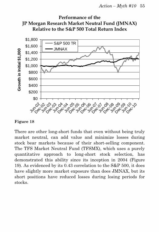
Action – Myth #10 55
Performance of the JP Morgan Research Market Neutral Fund (JMNAX)
Relative to the S&P 500 Total Return Index
There are other long-short funds that even without being truly
market neutral, can add value and minimize losses during
stock bear markets because of their short-selling component.
The TFS Market Neutral Fund (TFSMX), which uses a purely
quantitative approach to long-short stock selection, has
demonstrated this ability since its inception in 2004 (Figure
19). As evidenced by its 0.43 correlation to the S&P 500, it does
have slightly more market exposure than does JMNAX, but its
short positions have reduced losses during losing periods for
stocks.
$0
$200
$400
$600
$800
$1,000
$1,200
$1,400
$1,600
$1,800
Jun-
02
Dec
-02
Jun-
03
Dec
-03
Jun-
04
Dec
-04
Jun-
05
Dec
-05
Jun-
06
Dec
-06
Jun-
07
Dec
-07
Jun-
08
Dec
-08
Jun-
09
Dec
-09
Jun-
10
Dec
-10
Gro
wth
in
In
itia
l $
1,0
00
S&P 500 TR
JMNAX
Figure 18

56 Jackass Investing – Action for Myth #10
Performance of the TFS Market Neutral Fund (TFSMX)
Relative to the S&P 500 Total Return Index
Note: 10-1: Due to limitations on availability to new investors,
we have removed TFSMX from the portfolio. We have replaced
this market neutral constituent with TMNFX.
$0
$200
$400
$600
$800
$1,000
$1,200
$1,400
$1,600
$1,800
Dec
-04
Jun-
05
Dec
-05
Jun-
06
Dec
-06
Jun-
07
Dec
-07
Jun-
08
Dec
-08
Jun-
09
Dec
-09
Jun-
10
Dec
-10
Gro
wth
in
In
itia
l $
1,0
00
S&P 500 TR
TFSMX
Figure 19

57
Action – Myth #11
In this myth I introduced you to the term structure of
commodity futures contracts. The term structure is simply a
phrase that refers to the relationship in prices between futures
contracts that will be expiring soon and those that will not
expire for months or years to come. Because each of these
futures contract months trades at a price that is potentially
different from the other contract months, opportunities arise to
profit from these differences. One popular strategy that is
employed to capture this return driver, specifically in the
currency markets, is the “carry trade.”
The carry trade opportunity is created by the fact that interest
rates are at different levels in different countries. For example,
while the Australian one-year interest rate (how much you
would earn over the next twelve months if you purchased a
one-year Australian government note today) is at 5.75%, the
one-year Japanese interest rate is at 0.20%. This means that
an investor who borrows the equivalent of $1,000,000 in Japan
and buys a treasury note of the same value in Australia will
make $55,500 over the course of the year (person pays $2,000
in interest in Japan and earns $57,500 in interest in
Australia). The currency futures markets are priced to account
for this differential in interest rates between countries. The
futures contract for the Australian dollar one year in the future
is priced approximately 5.75% below today’s value of the
Australian dollar. This ensures that a person can’t simply buy
a one-year Australian note today, sell the Australian Dollar
futures contract (one-year forward) to hedge the currency risk
over the next year, and pocket the 5.75% risk-free. But by being
priced this way it enables a person to buy the one-year futures
contract, and, if the Australian Dollar remains at the same
level, profit from the fact that it will rise in price by 5.75% over
the next year. This is the basis for the carry trade.

58 Jackass Investing – Action for Myth #11
Many hedge funds and institutional investors frequently
engage in this carry trade. Because they have credit lines and
other means of borrowing, they may only post collateral of a
few percent of the face value of the borrowed money (certainly
less than $50,000), therefore earning more than 100% on their
invested funds.
There is of course a risk. Currency values fluctuate. If the
Japanese Yen increases in value by more than 5.55% over the
course of the year relative to the Australian Dollar, then the
entire profit is wiped out. That is because when the investor
pays back the $1,000,000 value of Japanese Yen that he
borrowed, it will actually cost 5.55% more, or $1,055,500. But
despite that risk of occasional loss, over time the carry trade
has produced positive returns.
Until recently, the use of this trading strategy has been
confined primarily to professional traders. But over the past
few years ETFs have been launched that provide people with
access to this strategy. One of those is the PowerShares DB
G10 Currency Harvest ETF (DBV). DBV seeks to track the
performance of the Deutsche Bank G10 Currency Future
Harvest Index – Excess Return, plus the U.S. short-term
interest rate. The fund compares the three-month interest
rates for each of the G10 currencies and then takes long
positions in the highest-yielding currencies and short positions
in the lowest-yielding currencies. Because this fund earns
returns from return drivers that are distinct from those that
drive the performance of most people’s portfolios, DBV can
provide portfolio diversification value.
Figure 20 shows the performance of the Deutsche Bank G10
Currency Future Harvest Index – Excess Return, starting in
1993, the first full year of its back-test, and extending through
September 2006 (reduced by 81 basis points per year to account
for the fees being charged to the ETF); and DBV since its first
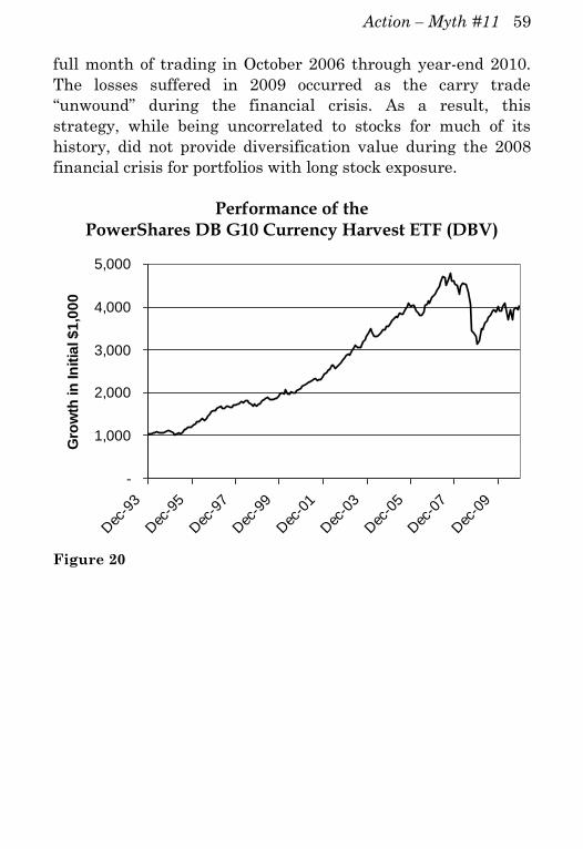
Action – Myth #11 59
full month of trading in October 2006 through year-end 2010.
The losses suffered in 2009 occurred as the carry trade
“unwound” during the financial crisis. As a result, this
strategy, while being uncorrelated to stocks for much of its
history, did not provide diversification value during the 2008
financial crisis for portfolios with long stock exposure.
Performance of the PowerShares DB G10 Currency Harvest ETF (DBV)
Figure 20
-
1,000
2,000
3,000
4,000
5,000
Dec
-93
Dec
-95
Dec
-97
Dec
-99
Dec
-01
Dec
-03
Dec
-05
Dec
-07
Dec
-09
Gro
wth
in
In
itia
l $
1,0
00

60
Action – Myth #12
We saw in Myth #12 how a diversified managed futures
portfolio, which I also refer to as “global trading,” can provide
more consistent returns with less risk than a portfolio
comprised of long positions in stocks, bonds and real estate.
This is because the commodity trading advisors (CTAs) that
trade these portfolios employ a broad range of trading
strategies to trade across hundreds of global stock index,
interest rate, energy, metals and agricultural markets. This
diversification, and the ability of CTAs to capture both up and
down market trends, is also why CTAs, in the aggregate,
produced profits during the 2008 financial crisis.
CTAs employ a wide variety of trading strategies to capture
profits from global trading. Some of the most popular methods
include:
Momentum (also called “trend following”): I discussed this in
Myth #7 – It’s Bad to Chase Performance. The propensity for
markets to trend is a key trading strategy underlying many
CTAs’ trading programs. It was the use of trend following
strategies in the currency, interest rate, stock index, energy,
metals and agricultural markets that contributed to the
substantial profits earned by CTAs during the financial crisis
of 2008.
Fundamentals: These trading strategies incorporate
fundamental market data, such as the cost-of-production data
used in the Marginal Cost of Production strategy described in
Myth #9. While this term is also used to refer to traders who
make discretionary decisions (do not follow a fully-systematic
investment process), I use it to describe systematic trading
strategies that base their trading decisions on data other than
market prices. Fundamental futures trading strategies are

Action – Myth #12 61
similar in concept to value or growth strategies used to select
stocks; with the difference being that fundamentally-based
futures strategies can be applied to raw commodities in
addition to stock indexes. This greatly expands the
diversification possibilities.
Relative Value, Yield Curves and Cross-rates: These strategies
all look at the relationship between or among two or more
markets to signal trading opportunities. A relative value
strategy may look at the prices of different futures contract
months for example, to determine that one contract should be
sold while another be purchased. Yield curve strategies may
buy long-term interest rate contracts and sell short short-term
interest rate contracts in the expectation that the yield curve
will steepen (short-term rates will rise in relation to long-term
rates). Cross-rates refer to the relationship among various
currencies. A trading strategy may buy the Euro while selling
the Japanese Yen (the currency carry trade described in Action
#11 utilizes cross-rate trading, but I’ve defined that as a
separate trading strategy). Relative value strategies are
similar in concept to market neutral strategies trading in
stocks, where some stocks are held long while other stocks are
sold short.
A key benefit of futures trading is that it allows a trader to
develop and incorporate dozens, or even hundreds, of different
trading strategies that can be applied across a hundred or more
global markets. While some CTAs specialize in a specific style
of trading (trend following being the most popular), there are
many CTAs that also diversify across both multiple trading
strategies and global markets. As a result, in creating the “Free
Lunch” portfolios that will be presented in the Action section
for Myth #20, I recommend a significant allocation to these
global trading strategies in any properly diversified portfolio.
(DISCLOSURE: although my firm, Brandywine Asset
Management, has experience trading in equities, private

62 Jackass Investing – Action for Myth #12
equity, mutual funds and ETFs, today our focus is solely on
futures trading. While we made this decision precisely because
we believe in the value futures trading can bring to a portfolio,
this focus may also create a bias in our belief in the necessity of
including managed futures in any truly diversified portfolio).
You can place money with a CTA either in an individually
managed account or fund. A managed account often requires at
least $100,000, and in many cases, more than $1,000,000 to
open. The high minimum investment level of the managed
account is required in order for the CTA to have enough assets
to fully diversify the account across a wide range of futures
markets. In contrast, managed futures funds, also called
“commodity pools,” combine peoples’ money into a single pooled
account. Unfortunately, most commodity pools are private and
limited to “Accredited Investors” only. This also means that the
funds cannot be publicly marketed; people need to “find” the
commodity pools on their own or be introduced to their
managers through a direct relationship. Most of these “private”
commodity pools also require relatively high initial
investments of $100,000 or more. However, in recent years a
number of commodity pools have publicly registered, enabling
people to make initial investments of as little as $1,000. A few
of the public funds available include:
Altegris Managed Futures Strategy O (MFTOX)
MutualHedge Futures Strategy C (MHFCX)
TFS Hedged Futures Fund (TFSHX)
Grant Park Managed Futures Strategy C (GPFCX)
Note 12-1: Due to limitations on availability to individual
investors, we have replaced MFTCX with MFTOX.

Action – Myth #12 63
In the Action section for Myth #20, I recommend a significant
allocation to these four funds or, alternatively, privately
managed accounts or funds that you can find through the
resources listed below, to provide your portfolio with valuable
global trading diversification.
Additional information on CTAs providing managed accounts
and private pools can be found at the following sources:
www.albourne.com: Albourne is a consultant, online
community and database provider to professional and private
investors.
www.autumngold.com: is a database provider specializing
in CTAs. The web site provides free access to CTA profiles and
performance information.
www.barclayhedge.com: BarclayHedge is one of the oldest
providers of CTA data, having been founded in 1985, and is the
developer of the BTOP 50 CTA index I presented in Myth #12.
In addition to its database services BarclayHedge provides
consultation to individuals and professional investors.
www.iasg.com: Institutional Advisory Services Group
assists clients in selecting CTAs that best match each client’s
risk tolerance and expected rates of return. The IASG website
provides access to a comprehensive database of CTAs and
hedge funds.
www.managedfutures.com: This is part of Altegris Group,
the manager of the Altegris Managed Futures Strategy Fund
mentioned previously. Altegris specializes in helping investors
discover and access managed futures programs and other
alternative investments. The web site contains access to a
database of CTAs.

64
Action – Myth #14
Myth #14 stresses that investors should not expect government
regulations to protect them from bad investments. I also
mention Alfred Winslow Jones and how the term “hedge fund”
was derived from the fact that he created the first fund that
“hedged” its long stock positions with offsetting short positions,
thereby creating a “hedged fund.” In this Action I will present a
description of what due diligence is and provide you with some
guidance that you should follow when evaluating an
investment opportunity.
Investment Due Diligence
Holly Miller, founder of Stone House Consulting and co-author
of the book The Top Ten Operational Risks: A Survival Guide
for Investment Management Firms and Hedge Funds, is an
expert on the practice of investment manager due diligence.
Due diligence is the process of asking about, and
understanding, the risks inherent in investing with an
investment manager or even a single investment. She has
provided the following advice regarding due diligence.
In general, the industry refers to two types of due diligence
that can be performed: investment due diligence and
operational due diligence, with the latter essentially including
everything that is not directly related to investment decision-
making. Many investors erroneously believe that each type of
due diligence can be performed independent of the other. Yet
without knowing about a manager’s approach toward
investing, it is impossible to assess whether the manager has
sufficient operational, compliance and IT infrastructure to
support the investment process. Likewise, without an
understanding of the manager’s operational processes,
investors cannot evaluate whether there are adequate controls
on the manager’s investment and trading activities.
Action – Myth #14 65
There is no single checklist that an investor can follow to
ensure he or she is asking an investment manager all the most
important questions. Depending on the answers received,
follow-up questions are often warranted. For example, if a
manager indicates they will not invest more than a specified
percentage of a portfolio in a given sector or industry, the
prudent investor will follow up by asking, “How do you monitor
that? What tools to you use? How often do you check? Do you
have a tolerance? Have you ever violated this restriction? Was
it intentional or inadvertent? How did it happen? How did you
find out you had made the error?”
Due diligence should always be performed before making an
investment. Yet ongoing due diligence is necessary to ensure
appropriate controls remain in place and that the manager has
adapted operational processes, systems and compliance
oversight based on regulatory changes, new product
introductions, staff turnover and market dynamics. At a
minimum, investors should revisit all due diligence reviews of
their managers on an annual basis and in some instances more
frequent reviews will be appropriate.
The devil is in the details and there is no easy short-cut to the
process. It is possible, though, to conduct due diligence in a way
that seeks to readily identify ‘red flags’ that would discourage
the manager from investing. Why continue to do your
homework on a manager you would avoid? Once enough red
flags are encountered, there is no need to complete an
exhaustive due diligence review. Instead, these flags signal
that it is time to move on to another potential opportunity. So
ask critical, ‘deal-breaker’ questions early in the process.
For this reason, most investors begin the due diligence process
on the investment side. If the manager’s investment approach,
philosophy and decision-making process – as well as the
manager’s track record – are insufficiently attractive, there is

66 Jackass Investing – Action for Myth #14
no point conducting any sort of operational due diligence
review.
Once a person has made the decision to pursue any investment,
they can then follow some basic Q & A guidelines. In the
United States, professional investment managers are generally
required to register either with the SEC or the CFTC
(Commodity Futures Trading Commission). These
organizations provide investors with some guidelines to follow.
You can see them at http://investor.gov/ask-questions/ and
http://www.nfa.futures.org/nfa-investor-information/index.html
67
Action – Myth #15
In June 2007, Roger Ibbotson, Zhiwu Chen and Wendy Hu
published a research paper titled “Liquidity as an Investment
Style.” In this paper they showed that less liquid stocks, those
that trade few shares relative to their earnings or shares
outstanding, outperform more liquid stocks. While you can
create your own portfolio of less liquid stocks by screening
stock databases to find those that have low trading volume
relative to their earnings and capitalization, you can now also
invest in mutual funds that do this for you.
Zebra Capital Management was founded in 2001 by Roger
Ibbotson and Zhiwu Chen and they launched a series of
products based on their Liquidity Return Strategy in 2009. In
2010 Zebra partnered with American Beacon Advisors to
launch two mutual funds based on this strategy. Those funds,
the American Beacon Large Cap Equity Fund (AZLPX) and the
American Beacon Zebra Small Cap Equity Fund (AZSPX),
began trading in June 2010. Although these two funds have
short performance histories, the research results displayed in
Myth #15, coupled with the back-tested results shown in
Figure 20 for the strategy (combining both small and large
capitalization stocks) prior to the start of trading in the mutual
funds, indicate that they could outperform the market averages
by a few percentage points per year. Because these are new
funds they also have only a few million dollars each in assets.
But if their research results is any guide, these two funds could
grow in size quite rapidly as their performance takes hold.
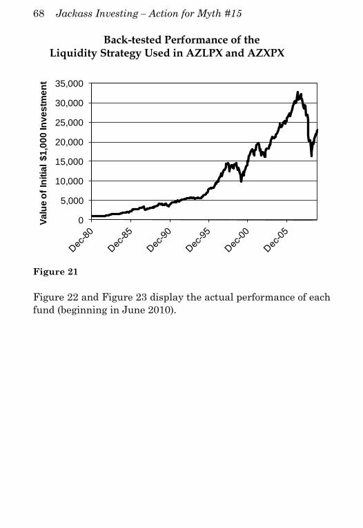
68 Jackass Investing – Action for Myth #15
Back-tested Performance of the Liquidity Strategy Used in AZLPX and AZXPX
Figure 22 and Figure 23 display the actual performance of each
fund (beginning in June 2010).
0
5,000
10,000
15,000
20,000
25,000
30,000
35,000
Va
lue
of
Init
ial
$1
,00
0 In
ve
stm
en
t
Figure 21
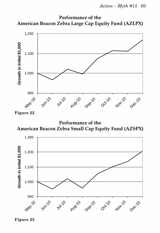
Action – Myth #15 69
Performance of the American Beacon Zebra Large Cap Equity Fund (AZLPX)
Performance of the American Beacon Zebra Small Cap Equity Fund (AZSPX)
900
1,000
1,100
1,200
1,300
May
-10
Jun-
10
Jul-1
0
Aug
-10
Sep
-10
Oct
-10
Nov
-10
Dec
-10
Gro
wth
in
In
itia
l $
1,0
00
900
1,000
1,100
1,200
May
-10
Jun-
10
Jul-1
0
Aug
-10
Sep
-10
Oct
-10
Nov
-10
Dec
-10
Gro
wth
in
In
itia
l $
1,0
00
Figure 22
Figure 23

70
Action – Myth #16
In Myth #16 I showed that simply buying-and-holding stocks
that are traded on exchanges or whose headquarters are based
in different countries provided very little diversification value,
especially in bear markets, as the country performances are
highly correlated with each other. But they are not perfectly
correlated and this opens up the opportunity to trade pursuant
to a disciplined strategy that attempts to identify and allocate
to the stocks domiciled in the strongest countries and avoid the
weakest. In Action #8 I presented a trading strategy developed
by Schreiner Capital Management (SCM), a registered
investment advisor, which followed a momentum-based
strategy of buying sector mutual funds that showed positive
price momentum. In this action I present a second strategy
developed by SCM to trade country-specific ETFs. Before I
present the strategy rules, let’s take a look at the performance
of the strategy relative to that of the MSCI All-World ex-USA
Index (Figure 24 and Figure 25). This performance has been
adjusted to reflect commissions of $0.01/share.

Action – Myth #16 71
Performance Comparison: International Allocation Strategy vs.
MSCI All-World ex-USA Index
Performance Comparison: International Allocation Strategy vs.
MSCI All-World ex-USA Index
MSCI All-World ex-USA
International Allocation Strategy
Years 11 11 Average Annual Return 1.39% 8.91% Annualized Volatility 19.21% 15.74% Maximum Drawdown -59% -33% % Profitable Months 56% 52% % Profitable Rolling 12-Mos. 62% 66% % Profitable Years 64% 64%
Figure 24. For the period January 2000 through December 2010
0
500
1,000
1,500
2,000
2,500
3,000
Va
lue
of
Init
ial
$1
,00
0 In
ve
stm
en
t
International Allocation Strategy
MSCI All -World ex-USA
Figure 25. For the period January 2000 through December 2010

72 Jackass Investing – Action for Myth #16
The performance shows that this simple momentum-based
strategy outperformed a buy-and-hold position in the MSCI All-
World ex-USA Index while suffering both lower volatility and
drawdowns.
International Allocation Strategy
The SCM International allocation strategy is a straightforward
momentum-based strategy that attempts to take long positions
in the strongest-performing country ETFs and avoid positions
in the weakest. The portfolio as defined by SCM includes 25
separate ETFs.
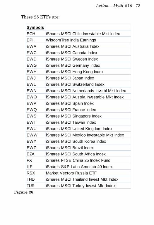
Action – Myth #16 73
Symbols
ECH iShares MSCI Chile Investable Mkt Index
EPI WisdomTree India Earnings
EWA iShares MSCI Australia Index
EWC iShares MSCI Canada Index
EWD iShares MSCI Sweden Index
EWG iShares MSCI Germany Index
EWH iShares MSCI Hong Kong Index
EWJ iShares MSCI Japan Index
EWL iShares MSCI Switzerland Index
EWN iShares MSCI Netherlands Invstbl Mkt Index
EWO iShares MSCI Austria Investable Mkt Index
EWP iShares MSCI Spain Index
EWQ iShares MSCI France Index
EWS iShares MSCI Singapore Index
EWT iShares MSCI Taiwan Index
EWU iShares MSCI United Kingdom Index
EWW iShares MSCI Mexico Investable Mkt Index
EWY iShares MSCI South Korea Index
EWZ iShares MSCI Brazil Index
EZA iShares MSCI South Africa Index
FXI iShares FTSE China 25 Index Fund
ILF iShares S&P Latin America 40 Index
RSX Market Vectors Russia ETF
THD iShares MSCI Thailand Invest Mkt Index
TUR iShares MSCI Turkey Invest Mkt Index
These 25 ETFs are:
Figure 26

74 Jackass Investing – Action for Myth #16
The basic underlying rule is to buy each ETF, selected from the
list, when it shows a positive rate of change (ROC) in price over
the prior 42 trading days. Each fund gets a 4% allocation of the
cash allocated to this strategy. Once a position is entered into it
is held in the strategy for a minimum of 21 trading days or
until the ROC turns negative.
Frontier Markets
In addition to employing a country allocation strategy, there is
one other area where a person can obtain some portfolio
diversification by placing money in stocks of other countries.
There are three levels of classification commonly used by
investment professionals to describe the status of the markets
of various countries. “Developed” countries, those such as the
United States, Germany and Japan, are well established and
very liquid. “Emerging” markets, such as Brazil, Russia and
Mexico, have lower trading activity and less well established
regulations than do the developed market countries. The final
classification, which refers to the countries with the smallest
stock market capitalizations and liquidity, are referred to as
“Frontier” markets. These include countries such as Vietnam,
Pakistan, and Jordan. Although the stock markets of frontier
markets are subject to the same emotional price moves as those
of both developed and emerging markets, they do tend to be
slightly less correlated to those markets. This is evidenced by
the 0.64 correlation of the frontier markets to the developed
markets and the 0.59 correlation of the frontier markets to the
emerging markets. In contrast, the developed markets and
emerging markets are 0.92 correlated with each other over the
same period.2 Because of this lower correlation we are
including a frontier markets mutual fund in our portfolio. This
is the Guggenheim Frontier Markets ETF (FRN). FRN has
approximately a 95% overlap with the MSCI EAFE Markets
Index.

Action – Myth #16 75
Note 16-1: The strategy algorithm was adjusted for results
beginning January 2011, so results in the book may differ
slightly from the results included in the Performance Reports
on the interactive website.
Note 16-2: As of January 2011, transaction costs are assumed
to be 0.10% per transaction.
2 Indexes and period used in the correlation calculations are
the monthly returns of the MSCI Frontier Markets Index,
MSCI Emerging Markets Index and MSCI All-World ex-USA
Index for the period June 2002 through December 2010.
76
Action – Myth #20
There is a free lunch in investing. It is the use of true portfolio
diversification. In this final (and most important) Action I will
show the specific trading strategies that combined to create the
performance of the Free Lunch portfolios presented in Myth
#20. These trading strategies, many of which have been
described in detail throughout this Action section, are based on
– and provide exposure to – more than two dozen separate
return drivers. As a result, unlike the composition of the
Conventional portfolio displayed in Myth #20, the Free Lunch
portfolios provide you with true portfolio diversification. In
order to provide model portfolios that can be used by a wide
range of investors, I have developed two types of Free Lunch
portfolios for you to select from; simplified and regular. The
only difference between the two is:
the “simplified” portfolio invests only in mutual funds
and ETFs, and does not trade them on an active basis.
the “regular” portfolio also includes individual stocks
and trades those as well as some of the ETFs.
In addition, each of the two portfolio types has the ability to
employ one of three levels of volatility:
Conservative: (this is the “regular” Free Lunch portfolio)
Moderate: “Free Lunch MR” (“MR” stands for “moderate
risk.” This portfolio matches the historical volatility of
the Conventional portfolio)
Aggressive: “Free Lunch AR” (“AR” stands for
“aggressive risk.” This portfolio matches the historical
volatility of the S&P 500)

Action – Myth #20 77
Before I describe the Free Lunch portfolios in detail, let’s take
a look at the constituents of what conventional financial
wisdom considers being portfolio diversification (Figure 27).
Conventional Portfolio Constituents
Knowing what we do now, after the facts presented in Myth
#16 – Allocate a Small Amount to Foreign Stocks,” Myth #17 –
Lower Risk by Diversifying Across Asset Classes, Myth #18 –
Diversification Failed in the 2008 Financial Crisis, and of
course Myth #20 – There is No Free Lunch, we can see that the
Conventional portfolio is a highly concentrated, non-diversified,
risky portfolio. As described in Myth #20, virtually all of its
returns are dependent on just three return drivers. In stark
contrast, the Free Lunch portfolios are much more properly
diversified, as illustrated in Figure 28.
Figure 27. The composition of the Conventional portfolio was
partially determined by looking at the allocations made by target-date
funds with approximately 20 years until retirement.
Large Cap U.S. Stocks
Mid Cap U.S. Stocks
Small Cap U.S. Stocks
Developed World Stocks
Emerging Markets Stocks
Aggregate U.S. Bonds
High Yield Bonds
Real Estate -U.S.
Cash

78 Jackass Investing – Action for Myth #20
Free Lunch Portfolio Diversification
A listing of each constituent and the percentage allocated to it
in the Free Lunch portfolios is provided in Figure 29. This table
also includes a listing of the actual investments you can make
to replicate the performance of the Free Lunch Portfolios, as
well as, if applicable, the number for the myth in which the
trading strategy underlying the investment was introduced.
You will notice that the last 18 listed trading strategies are
related to Myth #12. These are the “global trading” strategies
that can be accessed through investments in managed futures
accounts and funds. Although 18 separate return drivers are
identified, gaining exposure to these can be as simple as
investing in managed futures mutual funds (for smaller
portfolios) or private accounts (for larger portfolios). I identify
these later in this Action.
Figure 28. Use controls at bottom of frame to enlarge pie chart.
Large Cap - Static Long
Mid Cap - Static Long
Small Cap - Static Long
Developed World
Emerging Markets
Aggregate U.S. Bonds
High Yield
Real Estate - U.S.
Equal-Weighted Large Cap
Ind Corp Fundamentals
Dividend Increases
Insider Sentiment
Selective Small-cap Stocks
Selective Growth Stocks
Large Cap Liquidity
Small Cap Liquidity
Sector Timing
Market Timing - Country
Frontier Markets
Long International Bonds
Long-ShortMarket NeutralMarket Timing - Inv Sent
Credit & Equity Arbitrage
Currencies - Carry Trade
Currency - Momentum
Currency - Fundamentals
Currency - Cross-rates
Int Rates - Momentum
Int Rates - Fundamentals
Int Rates - Yield Curves
Stock Ind - Momentum
Stock Ind - Fundamentals
Stock Ind - Relative Value
Energy - Momentum
Energy - Fundamentals
Energy - Relative Value
Metals - Momentum
Metals - Fundamentals
Metals - Relative Value
Ags - Momentum
Ags - Fundamentals
Ags - Relative Value

Action – Myth #20 79
Exposure to Each Return Driver/Constituent of the Free Lunch Portfolio
Constituent Allocation Investment Myth
Cash 0.00%
Large Cap - Static Long 1.00% SPY
Mid Cap - Static Long 1.00% MDY
Small Cap - Static Long 1.00% IJR
Developed World 1.00% CWI
Emerging Markets 3.00% VWO
Aggregate U.S. Bonds 4.00% AGG
High Yield 4.00% JNK
Real Estate - U.S. 10.00% VNQ
Equal-Weighted Large Cap 1.00% RSP 4
Ind Corp Fundamentals 1.00% PRF 4
Dividend Increases 1.00% VIG 4
Insider Sentiment 1.00% NFO 4
Selective Small-cap Stocks 2.00% Piotroski Strategy 1
Selective Growth Stocks 2.00% CAN SLIM Strategy 6
Large Cap Liquidity 2.00% AZLPX 15
Small Cap Liquidity 2.00% AZSPX 15
Sector Timing 2.00% Trade Funds 8
Market Timing - International 2.00% Int'l ETF Strategy 16
Frontier Markets 3.00% FRN 16
Long International Bonds 4.00% BWX
Long-Short 5.00% TMNFX 10
Market Neutral 5.00% JMNAX.lw 10
Market Timing - Inv Sent 7.00% Trade SPY & SH 3
Credit & Equity Arbitrage 0.00% 14
Currencies - Carry Trade 3.00% DBV 11
Currency - Momentum 3.00% 12
Currency - Fundamentals 0.90% 12
Currency - Cross-rates 2.10% 12
Int Rates - Momentum 2.75% 12
Int Rates - Fundamentals 1.65% 12
Int Rates - Yield Curves 1.10% 12
Stock Ind - Momentum 2.75% 12
Stock Ind - Fundamentals 1.83% 12
Stock Ind - Relative Value 0.92% 12
Energy - Momentum 1.75% 12
Energy - Fundamentals 1.05% 12
Energy - Relative Value 0.70% 12
Metals - Momentum 2.00% 12
Metals - Fundamentals 1.20% 12
Metals - Relative Value 0.80% 12
Ags - Momentum 3.75% 12
Ags - Fundamentals 2.25% 12
Ags - Relative Value 1.50% 12
Als
o in
clu
de
d in
Co
nve
ntio
na
l p
ort
folio
Global Trading
Allocations can be made
to managed futures
accounts, private funds
or mutual funds, as
described in the
following section.
Figure 29

80 Jackass Investing – Action for Myth #20
Brief Description of the Constituents of the Free Lunch Portfolios That Are Not Separately Described in an Action
Large Cap – Static Long: SPY is an ETF that tracks the
mainstay of most people’s portfolios, a long position in the
stocks that make up the S&P 500.
Mid Cap – Static Long: MDY is an ETF that tracks the
performance of the S&P 400 Mid-cap Index.
Small Cap – Static Long: IJR is an ETF that tracks the
performance of the S&P 600 Small-cap Index.
Developed World: CWI is an ETF that tracks the performance
of the MSCI All-World (ex-USA) Index. This fund provides long
exposure to approximately 800 stocks in 22 developed countries
(such as Germany, Japan, and the U.K, but not the USA).
Emerging Markets: VWO is an ETF that tracks the
performance of the MSCI Emerging Markets Index. This fund
provides long exposure to approximately 700 stocks in 21
emerging countries (such as China, Brazil and Russia).
Aggregate U.S. Bonds: AGG is an ETF that tracks the
performance of the Barclay Aggregate Bond Index. This fund
provides exposure to more than 600 bonds.
High Yield: JNK is an ETF that tracks the performance of the
Barclay High Yield Very Liquid Index. This fund provides
exposure to approximately 200 bonds.
Real Estate – U.S.: VNQ is an ETF that tracks the performance
of the MSCI U.S. REIT Index. This fund provides exposure to
approximately 100 REITs.

Action – Myth #20 81
Description of the Constituents of the Global Trading Strategies Included in the Free Lunch Portfolios
In Action #12, I provided a brief description of the different
global trading strategies listed in the preceding table. There
are many more trading strategies that may fall outside of the
classifications listed in the table. There are also other methods
of obtaining the global trading diversification in the Free
Lunch portfolios in addition to investing with CTAs (which I
described in Action #12). But my experience with global trading
is through the use of futures contracts, which is why I
recommend managed futures as the source of global trading
diversification in the Free Lunch portfolios. The key is to make
sure that your portfolio contains a significant allocation to
trading strategies that produce returns that are independent of
each other. Managed futures (CTAs) provide this
diversification value. (DISCLOSURE: As I disclosed in Action
#12, although my firm, Brandywine Asset Management, has
experience trading in equities, private equity, mutual funds
and ETFs, today our focus is solely on managed futures
trading. While we made this decision precisely because we
believe in the value futures can bring to a portfolio, this focus
may also create a bias in our belief in the necessity of including
managed futures in any truly diversified portfolio).
Exposure to the global trading of currencies, interest rates,
stock indexes, energy, metals, and agricultural markets
described in this Action can be obtained in three different
ways. One is to identify individual funds or managers that
trade pursuant to each of the various trading strategies
represented in the global trading portion of the Free Lunch
portfolios and invest with them. The Free Lunch portfolio does
contain one such fund, DBV, which utilizes the currency carry
trading strategy described in Action #11. But there are few
other funds available to smaller investors that pursue

82 Jackass Investing – Action for Myth #20
individual global trading strategies, rendering this approach
problematic.
A second approach to gain exposure to the global trading
strategies is to establish the necessary brokerage accounts,
research and develop the strategies, and then trade them
yourself. I outlined one such “marginal cost of production”
trading strategy in Myth #9, and a simple momentum (also
called “trend following”) trading strategy in Action #7. But this
second approach is completely unrealistic for all but the most
well-capitalized and experienced investors. That is because
global trading in more than 100 markets (which is what is
represented in the Free Lunch portfolios) employing dozens of
trading strategies, is a professional pursuit. While today’s
technology allows some strategies, such as the momentum
strategy, to be executed by experienced traders on a part-time
basis, the full deployment of a diversified mix of global trading
strategies requires a full-time commitment and millions of
dollars in capital. It’s not as simple as tracking a single trading
strategy in stocks, such as the Piotroski trading strategy
described in Action #1.
A third approach, and the one I recommend for the vast
majority of investors, is to invest with one or more CTAs who
trade a broad range of global markets pursuant to a wide
variety of trading strategies. (Of course, as disclosed
previously, you must consider my bias, as this is the focus of
my firm.) There are hundreds of CTAs that in the aggregate
provide significant global trading diversification. I provide a
short list of services that provide information on these CTAs at
the end of Action #12. You can invest directly with these CTAs
in either managed accounts (generally requiring up to a million
dollars or more to obtain full diversification) or funds (which
allow substantially smaller minimum investments as they pool
your money with other investors). While most futures funds are
private (meaning they cannot be publicly advertised, but if you

Action – Myth #20 83
find them, they are often open to new investors), another option
has recently become available. As I mentioned in Myth #12,
there are mutual funds that employ the services of multiple
CTAs. For purposes of estimating the allocations to the various
global trading strategies in the Free Lunch portfolio, I assume
that the investor makes an equal allocation of 8% of their
portfolio to each of four managed futures mutual funds. These
are the MFTOX, MHFCX, TFSHX and GPFCX funds.
While this approach enables you to invest pursuant to the Free
Lunch portfolio, it is unable to be used in the Free Lunch MR
and Free Lunch AR portfolios. I will explain why, and how you
can do so, in the following section.
The Leveraged Free Lunch Portfolios
The Free Lunch MR and the Free Lunch AR portfolios hold the
same constituents as the regular Free Lunch portfolio, but with
an additional allocation to the global trading – managed
futures component. This additional allocation is made possible
without the use or cost of borrowed money. That is because
managed futures investors are able to use “notional” funds to
increase their exposure. Here’s how it works.
The typical managed futures account is required to hold cash
as a security deposit to maintain its positions. Although this is
also referred to as a “margin” requirement, it is different than
using margin to leverage a stock position. There is no
borrowing involved, nor interest required to be paid. A gold
futures contract, for example, obligates the buyer of that
contract to purchase 100 ounces of gold at a specified future
date (this is why it’s called a “futures” contract). The buyer can
sell that contract prior to that future date, thereby eliminating
the obligation to actually purchase the gold. In fact, this is
what occurs in the majority of futures transactions. Because
the buyer never actually owns the gold, only an obligation to
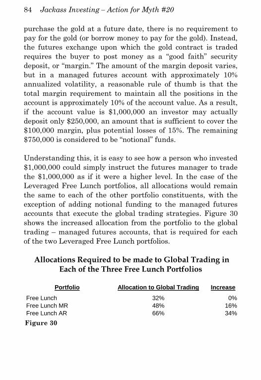
84 Jackass Investing – Action for Myth #20
purchase the gold at a future date, there is no requirement to
pay for the gold (or borrow money to pay for the gold). Instead,
the futures exchange upon which the gold contract is traded
requires the buyer to post money as a “good faith” security
deposit, or “margin.” The amount of the margin deposit varies,
but in a managed futures account with approximately 10%
annualized volatility, a reasonable rule of thumb is that the
total margin requirement to maintain all the positions in the
account is approximately 10% of the account value. As a result,
if the account value is $1,000,000 an investor may actually
deposit only $250,000, an amount that is sufficient to cover the
$100,000 margin, plus potential losses of 15%. The remaining
$750,000 is considered to be “notional” funds.
Understanding this, it is easy to see how a person who invested
$1,000,000 could simply instruct the futures manager to trade
the $1,000,000 as if it were a higher level. In the case of the
Leveraged Free Lunch portfolios, all allocations would remain
the same to each of the other portfolio constituents, with the
exception of adding notional funding to the managed futures
accounts that execute the global trading strategies. Figure 30
shows the increased allocation from the portfolio to the global
trading – managed futures accounts, that is required for each
of the two Leveraged Free Lunch portfolios.
Allocations Required to be made to Global Trading in Each of the Three Free Lunch Portfolios
Portfolio Allocation to Global Trading Increase
Free Lunch 32% 0%
Free Lunch MR 48% 16%
Free Lunch AR 66% 34%
Figure 30

Action – Myth #20 85
The investor would still maintain the same 68% allocation to
all other portfolio constituents. While investors in the Free
Lunch portfolio can use the four managed mutual funds
referenced in this Action to get their Global Trading exposure,
those funds do not allow a person to use notional funding.
Therefore, investors desiring to create one of the Leveraged
Free Lunch portfolios must do so by opening an individual
managed account, or by investing in a private managed futures
fund, that allows notional funding. Because the minimum
investment necessary for a manager to properly diversify a
managed account can exceed $1,000,000, this option is not
available to smaller investors. There are, however, a number of
managed futures funds that do provide investors with the
ability to invest substantially smaller amounts in a fund class
that is traded at a higher leverage level, thereby making those
funds suitable for inclusion in one of the Leveraged Free Lunch
portfolios.
The chart and table below illustrate the historical, back-tested
performance of the Free Lunch, Free Lunch MR and Free
Lunch AR portfolios compared with the Conventional portfolio.
The results shown in the chart and table below are based
on the portfolio compositions (constituents and weights)
outlined in the book. The historical back-tested results
of the current Free Lunch portfolio and current
Simplified Free Lunch portfolio will vary due to the
changes in the composition (constituents and weights) of
the portfolios as shown in Figure 29 and Figure 33.
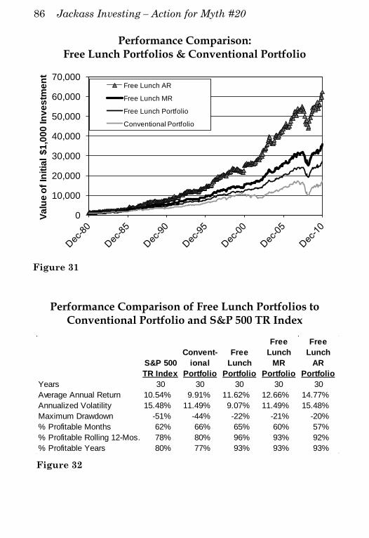
86 Jackass Investing – Action for Myth #20
Performance Comparison: Free Lunch Portfolios & Conventional Portfolio
Performance Comparison of Free Lunch Portfolios to
Conventional Portfolio and S&P 500 TR Index
0
10,000
20,000
30,000
40,000
50,000
60,000
70,000
Va
lue
of
Init
ial
$1
,00
0 In
ve
stm
en
t
Free Lunch AR
Free Lunch MR
Free Lunch Portfolio
Conventional Portfolio
S&P 500
TR Index
Convent-
ional
Portfolio
Free
Lunch
Portfolio
Free
Lunch
MR
Portfolio
Free
Lunch
AR
Portfolio
Years 30 30 30 30 30
Average Annual Return 10.54% 9.91% 11.62% 12.66% 14.77%
Annualized Volatility 15.48% 11.49% 9.07% 11.49% 15.48%
Maximum Drawdown -51% -44% -22% -21% -20%
% Profitable Months 62% 66% 65% 60% 57%
% Profitable Rolling 12-Mos. 78% 80% 96% 93% 92%
% Profitable Years 80% 77% 93% 93% 93%
Figure 31
Figure 32

Action – Myth #20 87
The Simplified Free Lunch Portfolios
Several constituents, including the five constituents of the Free
Lunch portfolios that require active trading, have been
removed from the Simplified Free Lunch portfolios in order to,
well, simplify them. The allocation made to these constituents
has been reallocated across trading strategies that provide the
most portfolio diversification value. A listing of each
constituent and the percentage allocated to it in the Simplified
Free Lunch portfolios is provided in Figure 33. Similar to the
composition of the Free Lunch portfolios displayed in Figure
29, this table also includes a listing of the actual investments
you can make to replicate the performance of the Free Lunch
Portfolios, as well as, if applicable, the number for the myth in
which the trading strategy underlying the investment was
introduced. Exposure to the 36% allocated to the global trading
can be achieved with equal 9% investments in each of four
managed futures mutual funds. These are the MFTOX,
MHFCX, TFSHX and GPFCX funds.

88 Jackass Investing – Action for Myth #20
Exposure to Each Return Driver/Constituent of the Simplified Free Lunch Portfolio
Constituent Allocation Investment Myth
Cash 0.00%
Developed World 5.00% CWI
Emerging Markets 6.00% VWO
Aggregate U.S. Bonds 7.00% AGG
Real Estate - U.S. 12.00% VNQ
Equal-Weighted Large Cap 5.00% RSP 4
Frontier Markets 6.00% FRN 16
Long International Bonds 7.00% BWX
Long-Short 6.00% TMNFX 10
Market Neutral 6.00% JMNAX.lw 10
Currencies - Carry Trade 4.00% DBV 11
Currency - Momentum 3.38% 12
Currency - Fundamentals 1.01% 12
Currency - Cross-rates 2.36% 12
Int Rates - Momentum 3.09% 12
Int Rates - Fundamentals 1.86% 12
Int Rates - Yield Curves 1.24% 12
Stock Ind - Momentum 3.09% 12
Stock Ind - Fundamentals 2.06% 12
Stock Ind - Relative Value 1.03% 12
Energy - Momentum 1.97% 12
Energy - Fundamentals 1.18% 12
Energy - Relative Value 0.79% 12
Metals - Momentum 2.25% 12
Metals - Fundamentals 1.35% 12
Metals - Relative Value 0.90% 12
Ags - Momentum 4.22% 12
Ags - Fundamentals 2.53% 12
Ags - Relative Value 1.69% 12
Als
o incl in
Conv p
ort
Global Trading
Allocations can be made
to managed futures
accounts, private funds
or mutual funds, as
previously described.
Figure 33
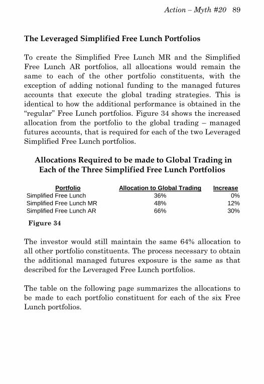
Action – Myth #20 89
The Leveraged Simplified Free Lunch Portfolios
To create the Simplified Free Lunch MR and the Simplified
Free Lunch AR portfolios, all allocations would remain the
same to each of the other portfolio constituents, with the
exception of adding notional funding to the managed futures
accounts that execute the global trading strategies. This is
identical to how the additional performance is obtained in the
“regular” Free Lunch portfolios. Figure 34 shows the increased
allocation from the portfolio to the global trading – managed
futures accounts, that is required for each of the two Leveraged
Simplified Free Lunch portfolios.
Allocations Required to be made to Global Trading in Each of the Three Simplified Free Lunch Portfolios
The investor would still maintain the same 64% allocation to
all other portfolio constituents. The process necessary to obtain
the additional managed futures exposure is the same as that
described for the Leveraged Free Lunch portfolios.
The table on the following page summarizes the allocations to
be made to each portfolio constituent for each of the six Free
Lunch portfolios.
Portfolio Allocation to Global Trading Increase
Simplified Free Lunch 36% 0%
Simplified Free Lunch MR 48% 12%
Simplified Free Lunch AR 66% 30%
Figure 34

90 Jackass Investing – Action for Myth #20
Summary of the Allocations to be Made to Each Constituent of Each Portfolio
Note to Global Trading / Managed Futures exposure in the
“MR” and “AR” portfolios:
(1) The additional exposure to global trading / managed futures
is obtained by placing an amount of cash up to that
available (the "Cash Level") in a leveraged managed futures
account or fund that provides the exposure equal to the
"Trading Level." Target returns on the Trading Level
should be 10% - 12%.
Constituent Myth Investment
Cash 0.00% 0.00% 0.00% 0.00% 0.00% 0.00%
Large Cap - Static Long SPY 1.00% 1.00% 1.00% 0.00% 0.00% 0.00%
Mid Cap - Static Long MDY 1.00% 1.00% 1.00% 0.00% 0.00% 0.00%
Small Cap - Static Long IJR 1.00% 1.00% 1.00% 0.00% 0.00% 0.00%
Developed World CWI 1.00% 1.00% 1.00% 5.00% 5.00% 5.00%
Emerging Markets VWO 3.00% 3.00% 3.00% 6.00% 6.00% 6.00%
Aggregate U.S. Bonds AGG 4.00% 4.00% 4.00% 7.00% 7.00% 7.00%
High Yield JNK 4.00% 4.00% 4.00% 0.00% 0.00% 0.00%
Real Estate - U.S. VNQ 10.00% 10.00% 10.00% 12.00% 12.00% 12.00%
Equal-Weighted Large Cap 4 RSP 1.00% 1.00% 1.00% 5.00% 5.00% 5.00%
Ind Corp Fundamentals 4 PRF 1.00% 1.00% 1.00% 0.00% 0.00% 0.00%
Dividend Increases 4 VIG 1.00% 1.00% 1.00% 0.00% 0.00% 0.00%
Insider Sentiment 4 NFO 1.00% 1.00% 1.00% 0.00% 0.00% 0.00%
Selective Small-cap Stocks 1 Piotroski Strategy 2.00% 2.00% 2.00% 0.00% 0.00% 0.00%
Selective Growth Stocks 6 CAN SLIM Strategy 2.00% 2.00% 2.00% 0.00% 0.00% 0.00%
Large Cap Liquidity 15 AZLPX 2.00% 2.00% 2.00% 0.00% 0.00% 0.00%
Small Cap Liquidity 15 AZSPX 2.00% 2.00% 2.00% 0.00% 0.00% 0.00%
Sector Timing 8 Trade Funds 2.00% 2.00% 2.00% 0.00% 0.00% 0.00%
Market Timing - International 16 Int'l ETF Strategy 2.00% 2.00% 2.00% 0.00% 0.00% 0.00%
Frontier Markets 16 FRN 3.00% 3.00% 3.00% 6.00% 6.00% 6.00%
Long International Bonds BWX 4.00% 4.00% 4.00% 7.00% 7.00% 7.00%
Long-Short 10 TMNFX 5.00% 5.00% 5.00% 6.00% 6.00% 6.00%
Market Neutral 10 JMNAX.lw 5.00% 5.00% 5.00% 6.00% 6.00% 6.00%
Market Timing - Inv Sent 3 Trade SPY & SH 7.00% 7.00% 7.00% 0.00% 0.00% 0.00%
Credit & Equity Arbitrage 14 0.00% 0.00% 0.00% 0.00% 0.00% 0.00%
Currencies - Carry Trade 11 DBV 3.00% 3.00% 3.00% 4.00% 4.00% 4.00%
12 MFTOX 8.00% 9.00%
12 MHFCX 8.00% 9.00%
12 TFSHX 8.00% 9.00%
12 GPFCX 8.00% 9.00%
Global Trading / Managed
Futures (1)
Simplified
Free
Lunch
Simplified
Free
Lunch MR
Als
o inclu
ded in
Conventional port
folio
Free
Lunch
Simplified
Free
Lunch AR
(1) Cash
Level: 32%
Trading
Level: 48%
(1) Cash
Level: 32%
Trading
Level: 66%
(1) Cash
Level: 36%
Trading
Level: 48%
(1) Cash
Level: 36%
Trading
Level: 66%
Free
Lunch MR
Free
Lunch AR
Figure 35.