jan 23, 2003computational gene finding1 sanja rogic cs department ubc
Post on 19-Dec-2015
214 views
TRANSCRIPT
Jan 23, 2003 Computational Gene Finding 1
Computational Gene Finding
Sanja RogicCS Department UBC
Jan 23, 2003 Computational Gene Finding 2
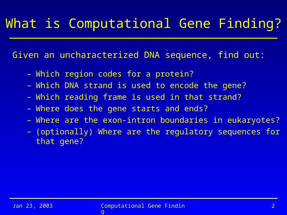
What is Computational Gene Finding?
Given an uncharacterized DNA sequence, find out:
– Which region codes for a protein?– Which DNA strand is used to encode the gene?– Which reading frame is used in that strand?– Where does the gene starts and ends?– Where are the exon-intron boundaries in eukaryotes?– (optionally) Where are the regulatory sequences for that
gene?

Jan 23, 2003 Computational Gene Finding 3
Prokaryotic Vs. Eukaryotic Gene Finding
Prokaryotes:
• small genomes 0.5 – 10·106 bp
• high coding density (>90%)• no introns
– Gene identification relatively easy, with success rate ~ 99%
Problems:
• overlapping ORFs• short genes• finding TSS and promoters
Eukaryotes:
• large genomes 107 – 1010 bp• low coding density (<50%)• intron/exon structure
– Gene identification a complex problem, gene level accuracy ~50%
Problems:• many

Jan 23, 2003 Computational Gene Finding 4
Gene Structure

Jan 23, 2003 Computational Gene Finding 5
Gene Finding: Different Approaches
• Similarity-based methods (extrinsic) - use similarity to annotated sequences:
– proteins– cDNAs– ESTs
• Comparative genomics - Aligning genomic sequences from different species
• Ab initio gene-finding (intrinsic)
• Integrated approaches

Jan 23, 2003 Computational Gene Finding 6
Similarity-based methods
• Based on sequence conservation due to functional constraints
• Use local alignment tools (Smith-Waterman algo, BLAST, FASTA) to search protein, cDNA, and EST databases
• Will not identify genes that code for proteins not already in databases (can identify ~50% new genes)
• Limits of the regions of similarity not well defined
Jan 23, 2003 Computational Gene Finding 7
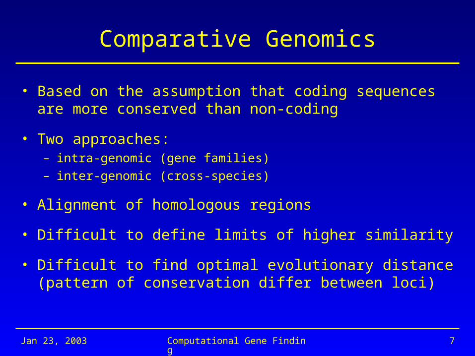
Comparative Genomics
• Based on the assumption that coding sequences are more conserved than non-coding
• Two approaches:– intra-genomic (gene families)– inter-genomic (cross-species)
• Alignment of homologous regions
• Difficult to define limits of higher similarity
• Difficult to find optimal evolutionary distance (pattern of conservation differ between loci)

Jan 23, 2003 Computational Gene Finding 8

Jan 23, 2003 Computational Gene Finding 9
Summary for Extrinsic Approaches
Strengths:
• Rely on accumulated pre-existing biological data, thus should produce biologically relevant predictions
Weaknesses:
• Limited to pre-existing biological data• Errors in databases• Difficult to find limits of similarity
Jan 23, 2003 Computational Gene Finding 10
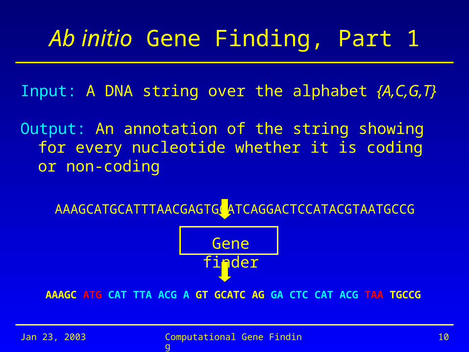
Ab initio Gene Finding, Part 1
Input: A DNA string over the alphabet {A,C,G,T}
Output: An annotation of the string showing for every nucleotide whether it is coding or non-coding
AAAGCATGCATTTAACGAGTGCATCAGGACTCCATACGTAATGCCG
AAAGC ATG CAT TTA ACG A GT GCATC AG GA CTC CAT ACG TAA TGCCG
Gene finder
Jan 23, 2003 Computational Gene Finding 11
Ab initio Gene Finding, Part 2
• Using only sequence information
• Identifying only coding exons of protein-coding genes (transcription start site, 5’ and 3’ UTRs are ignored)
• Integrates coding statistics with signal detection

Jan 23, 2003 Computational Gene Finding 12
Coding Statistics, Part 1
• Unequal usage of codons in the coding regions is a universal feature of the genomes
– uneven usage of amino acids in existing proteins– uneven usage of synonymous codons (correlates with the
abundance of corresponding tRNAs)
• We can use this feature to differentiate between coding and non-coding regions of the genome
• Coding statistics - a function that for a given DNA sequence computes a likelihood that the sequence is coding for a protein
Jan 23, 2003 Computational Gene Finding 13
Coding Statistics, Part 2
• Many different ones
– codon usage– hexamer usage– GC content– compositional bias between codon positions– nucleotide periodicity– …
Jan 23, 2003 Computational Gene Finding 14
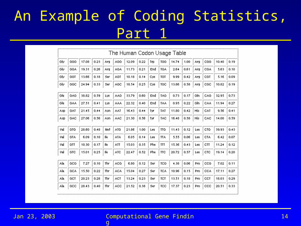
An Example of Coding Statistics, Part 1
Jan 23, 2003 Computational Gene Finding 15
An Example of Coding Statistics, Part 2
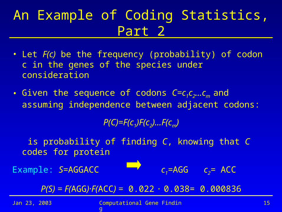
• Let F(c) be the frequency (probability) of codon c in the genes of the species under consideration
• Given the sequence of codons C=c1c2…cm and assuming independence between adjacent codons:
P(C)=F(c1)F(c2)…F(cm)
is probability of finding C, knowing that C codes for protein
Example: S=AGGACC c1=AGG c2= ACC
P(S) = F(AGG)·F(ACC) = 0.022 · 0.038= 0.000836
Jan 23, 2003 Computational Gene Finding 16
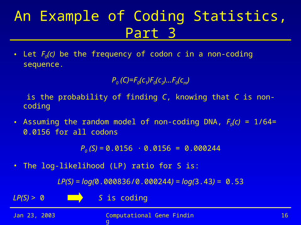
An Example of Coding Statistics, Part 3
• Let F0(c) be the frequency of codon c in a non-coding sequence.
P0 (C)=F0(c1)F0(c2)…F0(cm)
is the probability of finding C, knowing that C is non-coding
• Assuming the random model of non-coding DNA, F0(c) = 1/64= 0.0156 for all codons
P0 (S) = 0.0156 · 0.0156 = 0.000244
• The log-likelihood (LP) ratio for S is:
LP(S) = log(0.000836/0.000244) = log(3.43) = 0.53
LP(S) > 0 S is coding

Jan 23, 2003 Computational Gene Finding 17
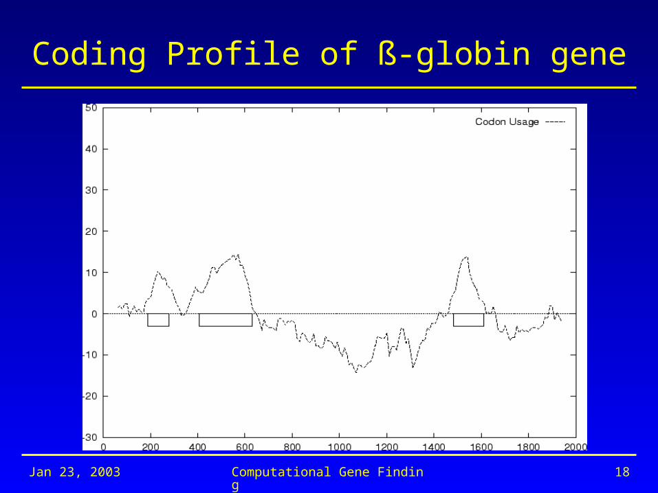
Computing Coding Statistics in Practice
• Usually, the value of coding statistics is computed using sliding windows coding profile of the sequence
• Larger windows are required to detect a clear signal (50 – 200 bp)
Jan 23, 2003 Computational Gene Finding 18
Coding Profile of ß-globin gene
Jan 23, 2003 Computational Gene Finding 19
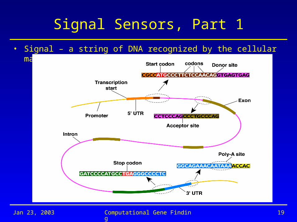
Signal Sensors, Part 1
• Signal – a string of DNA recognized by the cellular machinery
Jan 23, 2003 Computational Gene Finding 20
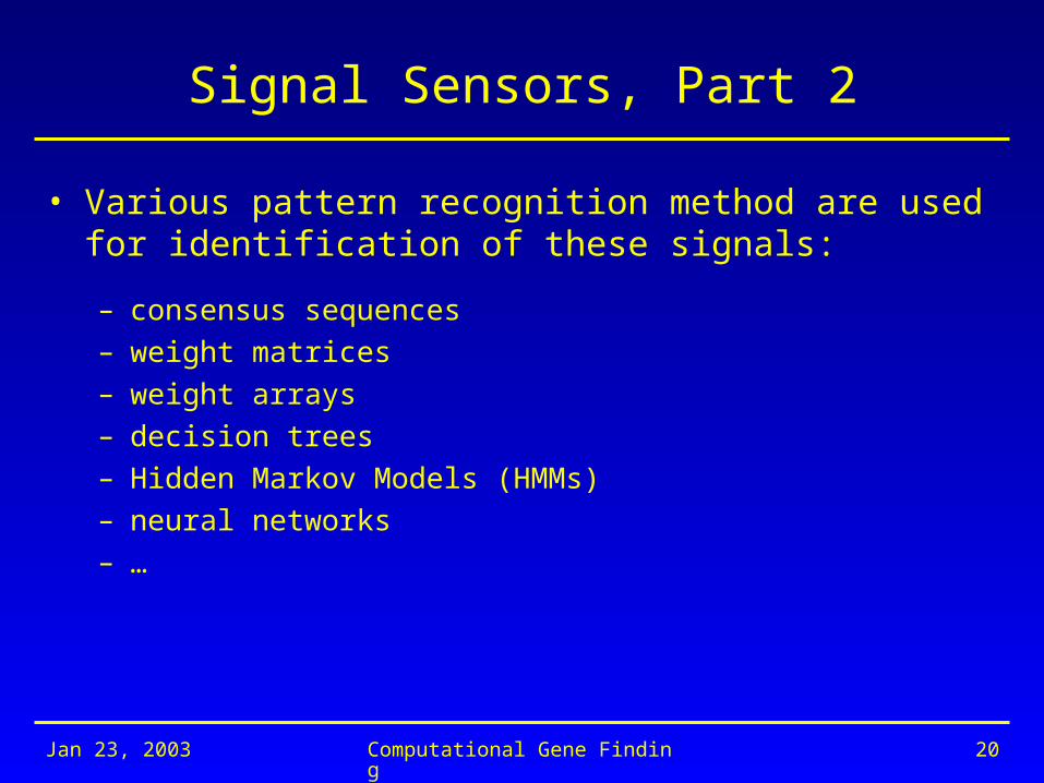
Signal Sensors, Part 2
• Various pattern recognition method are used for identification of these signals:
– consensus sequences– weight matrices– weight arrays– decision trees– Hidden Markov Models (HMMs)– neural networks– …

Jan 23, 2003 Computational Gene Finding 21
Example of Consensus Sequence
• obtained by choosing the most frequent base at each position of the multiple alignment of subsequences of interest
TACGATTATAATTATAATGATACTTATGATTATGTT
consensus sequence
consensus (IUPAC)
Leads to loss of information and can produce many false positive or false negative predictions
TATAAT
TATRNT
MELONMANGOHONEYSWEETCOOKY
MONEY
Jan 23, 2003 Computational Gene Finding 22
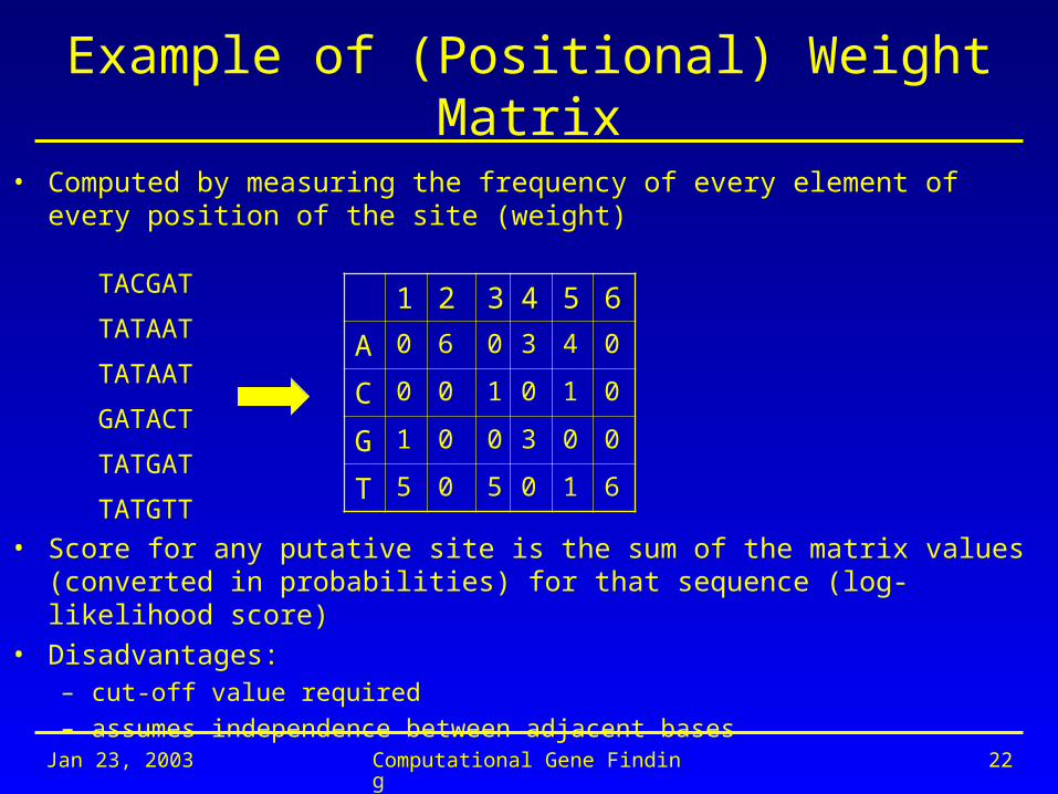
Example of (Positional) Weight Matrix
• Computed by measuring the frequency of every element of every position of the site (weight)
• Score for any putative site is the sum of the matrix values (converted in probabilities) for that sequence (log-likelihood score)
• Disadvantages: – cut-off value required– assumes independence between adjacent bases
TACGAT
TATAAT
TATAAT
GATACT
TATGAT
TATGTT
1 2 3 4 5 6
A 0 6 0 3 4 0
C 0 0 1 0 1 0
G 1 0 0 3 0 0
T 5 0 5 0 1 6

Jan 23, 2003 Computational Gene Finding 23
Example of Decision Tree
Jan 23, 2003 Computational Gene Finding 24
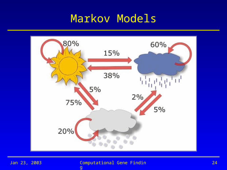
Markov Models
Jan 23, 2003 Computational Gene Finding 25
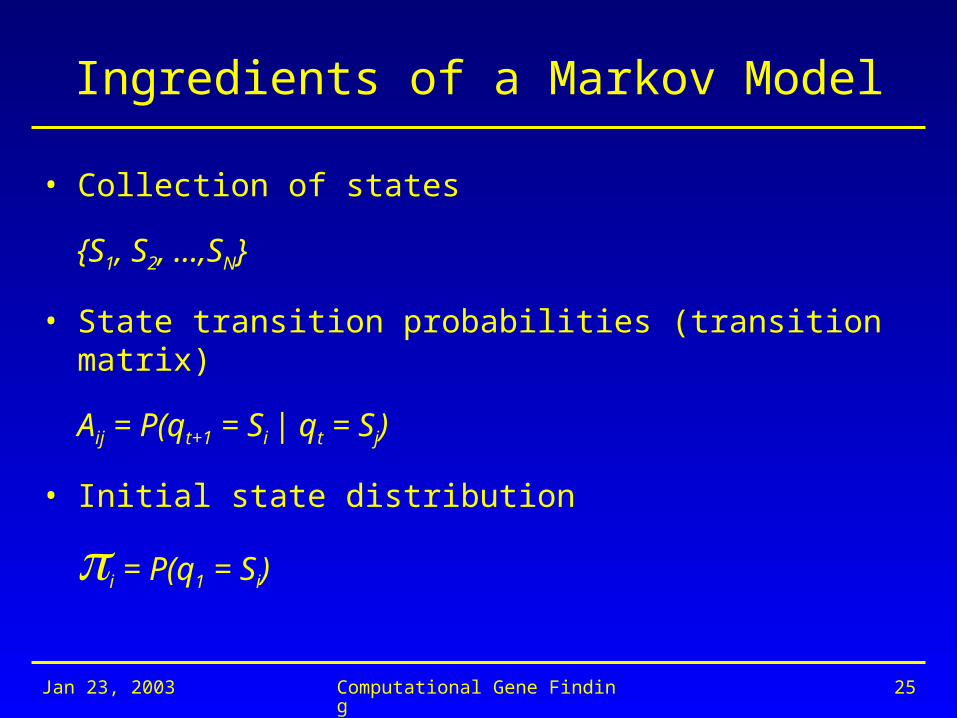
Ingredients of a Markov Model
• Collection of states
{S1, S2, …,SN}
• State transition probabilities (transition matrix)
Aij = P(qt+1 = Si | qt = Sj)
• Initial state distribution
i = P(q1 = Si)
Jan 23, 2003 Computational Gene Finding 26
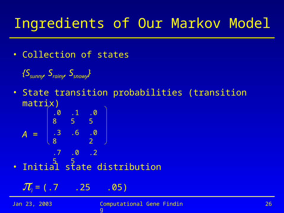
Ingredients of Our Markov Model
• Collection of states
{Ssunny, Srainy, Ssnowy}
• State transition probabilities (transition matrix)
A =
• Initial state distribution
i = (.7 .25 .05)
.08 .15 .05
.38 .6 .02
.75 .05 .2

Jan 23, 2003 Computational Gene Finding 27
Probability of a Sequence of Events
P(Ssunny) x P(Srainy | Ssunny) x P(Srainy | Srainy) x
P(Srainy | Srainy) x P(Ssnowy | Srainy) x P(Ssnowy | Ssnowy)
= 0.7 x 0.15 x 0.6 x 0.6 x 0.02 x 0.2 = 0.0001512

Jan 23, 2003 Computational Gene Finding 28
Hidden Markov Models
Jan 23, 2003 Computational Gene Finding 29
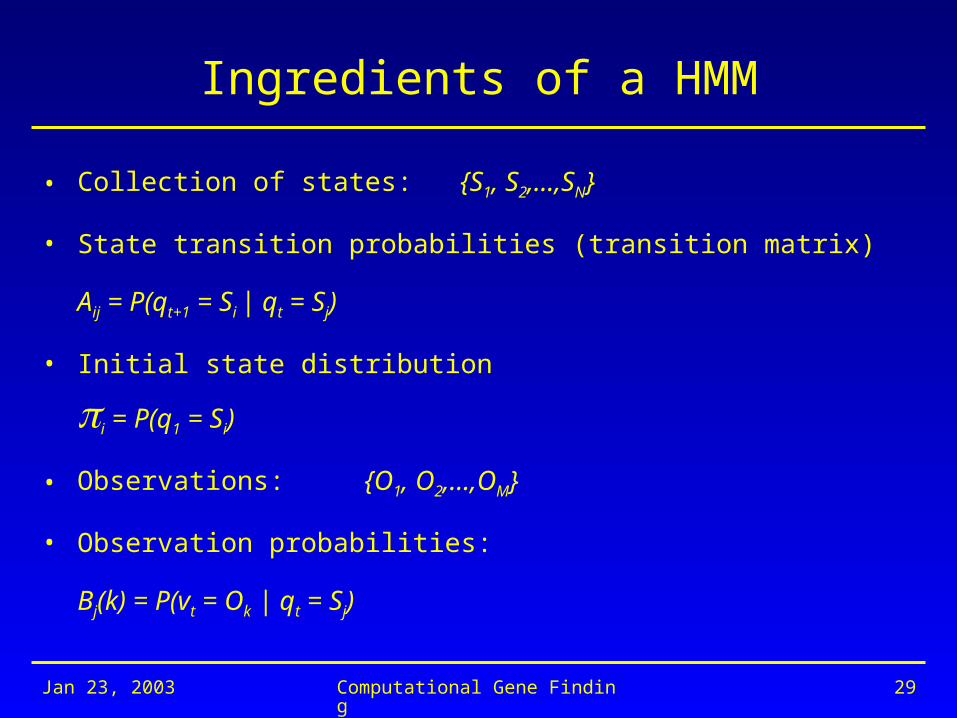
Ingredients of a HMM
• Collection of states: {S1, S2,…,SN}
• State transition probabilities (transition matrix)
Aij = P(qt+1 = Si | qt = Sj)
• Initial state distribution
i = P(q1 = Si)
• Observations: {O1, O2,…,OM}
• Observation probabilities:
Bj(k) = P(vt = Ok | qt = Sj)
Jan 23, 2003 Computational Gene Finding 30
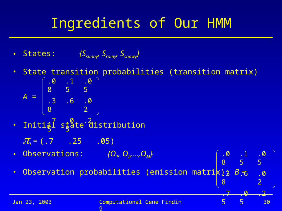
Ingredients of Our HMM
• States:{Ssunny, Srainy, Ssnowy}
• State transition probabilities (transition matrix)
A =
• Initial state distribution
i = (.7 .25 .05)
• Observations: {O1, O2,…,OM}
• Observation probabilities (emission matrix): B =
.08 .15 .05
.38 .6 .02
.75 .05 .2
.08 .15 .05
.38 .6 .02
.75 .05 .2
Jan 23, 2003 Computational Gene Finding 31
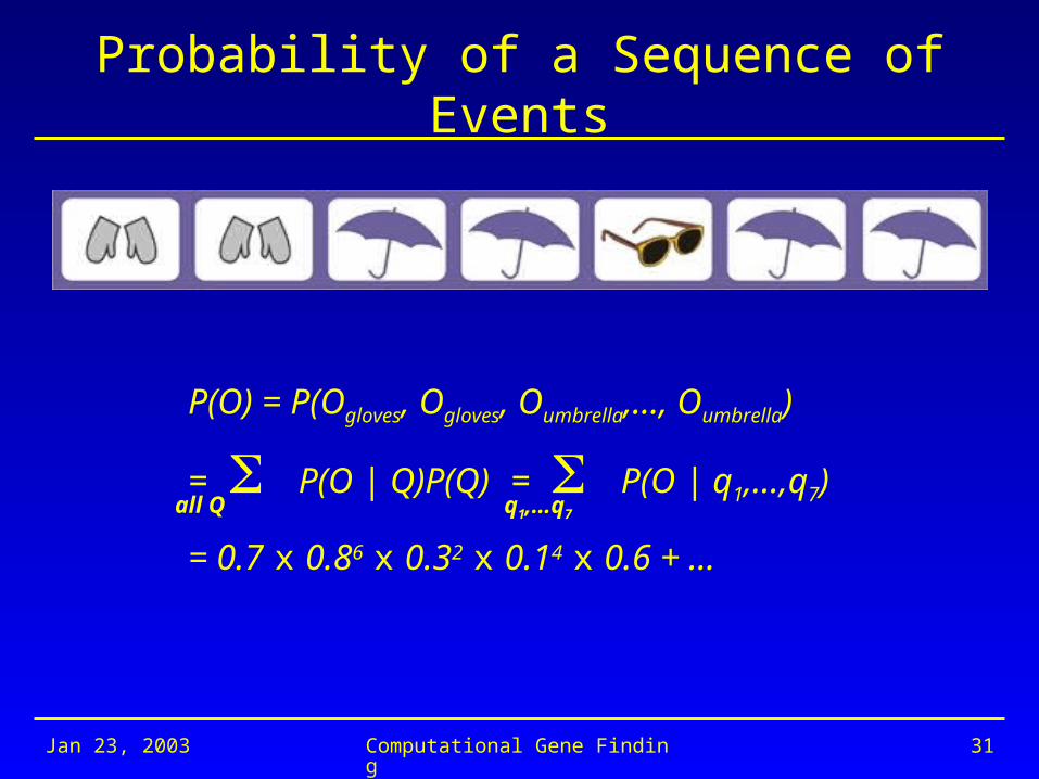
Probability of a Sequence of Events
P(O) = P(Ogloves, Ogloves, Oumbrella,…, Oumbrella)
= P(O | Q)P(Q) = P(O | q1,…,q7)
= 0.7 x 0.86 x 0.32
x 0.14 x 0.6 + …
all Q q1,…q7
Jan 23, 2003 Computational Gene Finding 32
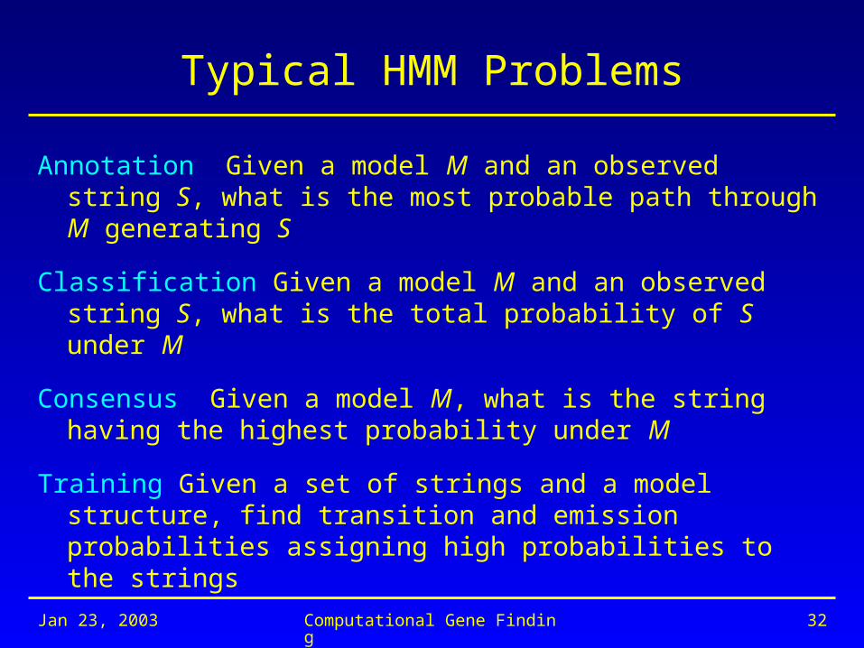
Typical HMM Problems
Annotation Given a model M and an observed string S, what is the most probable path through M generating S
Classification Given a model M and an observed string S, what is the total probability of S under M
Consensus Given a model M, what is the string having the highest probability under M
Training Given a set of strings and a model structure, find transition and emission probabilities assigning high probabilities to the strings

Jan 23, 2003 Computational Gene Finding 33
HMMs and Gene Structure
• Nucleotides {A,C,G,T} are the observables
• Different states generates generate nucleotides at different frequencies
A simple HMM for unspliced genes:
AAAGC ATG CAT TTA ACG AGA GCA CAA GGG CTC TAA TGCCG• The sequence of states is an annotation of the generated string –
each nucleotide is generated in intergenic, start/stop, coding state

Jan 23, 2003 Computational Gene Finding 34
State of the Art in Ab initio Gene Finding
• Coding statistics and signal sensors are integrated in overall gene model using
– machine learning techniques (HMMs, decision trees, neural networks)
– discriminant functions (linear, quadratic)
• Use dynamic programming (Viterbi) to find the highest scoring path through the model
• Capable of predicting:
– genes on both strands simultaneously– partial and multiple genes in a sequence– suboptimal exons

Jan 23, 2003 Computational Gene Finding 35
Examples of Gene Finders
FGENES – linear DF for content and signal sensors and DP for finding optimal combination of exons
GeneMark – HMMs enhanced with ribosomal binding site recognition
Genie – neural networks for splicing, HMMs for coding sensors, overall structure modeled by HMM
Genscan – WM, WA and decision trees as signal sensors, HMMs for content sensors, overall HMM
HMMgene – HMM trained using conditional maximum likelihood
Morgan – decision trees for exon classification, also Markov Models
MZEF – quadratic DF, predict only internal exons

Jan 23, 2003 Computational Gene Finding 36
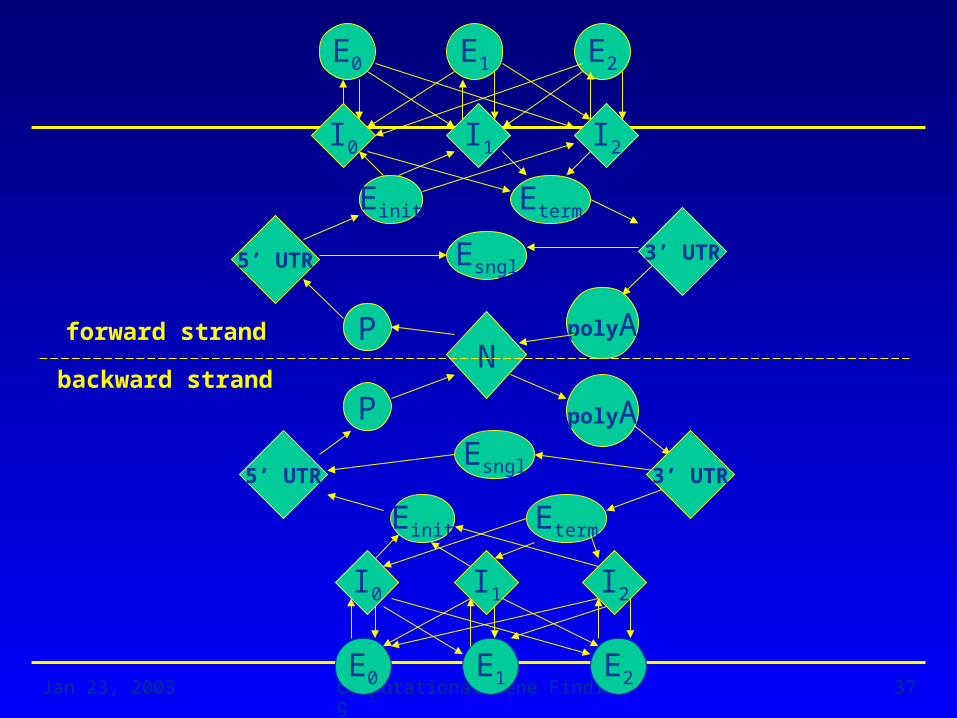
Genscan Example
• Developed by Chris Burge 1997
• One of the most accurate ab initio programs
• Uses explicit state duration HMM to model gene structure (different length distributions for exons)
• Different model parameters for regions with different GC content
37Computational Gene FindingJan 23, 2003
E0 E1 E2
E2E1E0
NP
Eterm
P
Einit
polyA
5’ UTR
I0 I1 I2
I0 I1 I2
Esngl
Esngl
Einit Eterm
forward strand
backward strand
3’ UTR
5’ UTR 3’ UTR
polyA

Jan 23, 2003 Computational Gene Finding 38
Genscan’s Architecture
• HMM’s states for exons and introns in three different phases, single exon, 5’ and 3’ UTRs, promoter region and polyA site and intergenic region
• Explicit length modeling
• HMMs for exons, introns and intergenic regions
• WM and WA for acceptor site, branch point, polyA site and promoter region
• Decision tree (maximal dependence decomposition) for donor sites

Jan 23, 2003 Computational Gene Finding 39
Ab initio Gene Finding is Difficult
• Genes are separated by large intergenic regions
• Genes are not continuous, but split in a number of (small) coding exons, separated by (larger) non-coding introns
– in humans coding sequence comprise only a few percents of the genome and an average of 5% of each gene
• Sequence signals that are essential for elucidation of a gene structure are degenerate and highly unspecific
• Alternative splicing
• Repeat elements (>50% in humans) – some contain coding regions
Jan 23, 2003 Computational Gene Finding 40
Problems with Ab initio Gene Finding
• No biological evidence
• In long genomic sequences many false positive predictions
• Prediction accuracy high, but not sufficient
Jan 23, 2003 Computational Gene Finding 41
Evaluation of Gene Finding Programs
• Calculating accuracy of programs’ predictions
• Several evaluation studies:
– Burset and Guigó, 1996 (vertebrate sequences)– Pavy et al., 1999 (Arabidopsis thaliana)– Rogic et al., 2001 (mammalian sequences)

Jan 23, 2003 Computational Gene Finding 42
Measures of Prediction Accuracy, Part 1
Nucleotide level accuracy
Sensitivity =
Specificity =
TN FPFN TN TNTPFNTP FN
REALITY
PREDICTION
number of correct exonsnumber of actual exons
number of correct exonsnumber of predicted exons

Jan 23, 2003 Computational Gene Finding 43
Measures of Prediction Accuracy, Part 2
Exon level accuracy
REALITY
PREDICTION
WRONGEXON
CORRECTEXON
MISSINGEXON
Jan 23, 2003 Computational Gene Finding 44
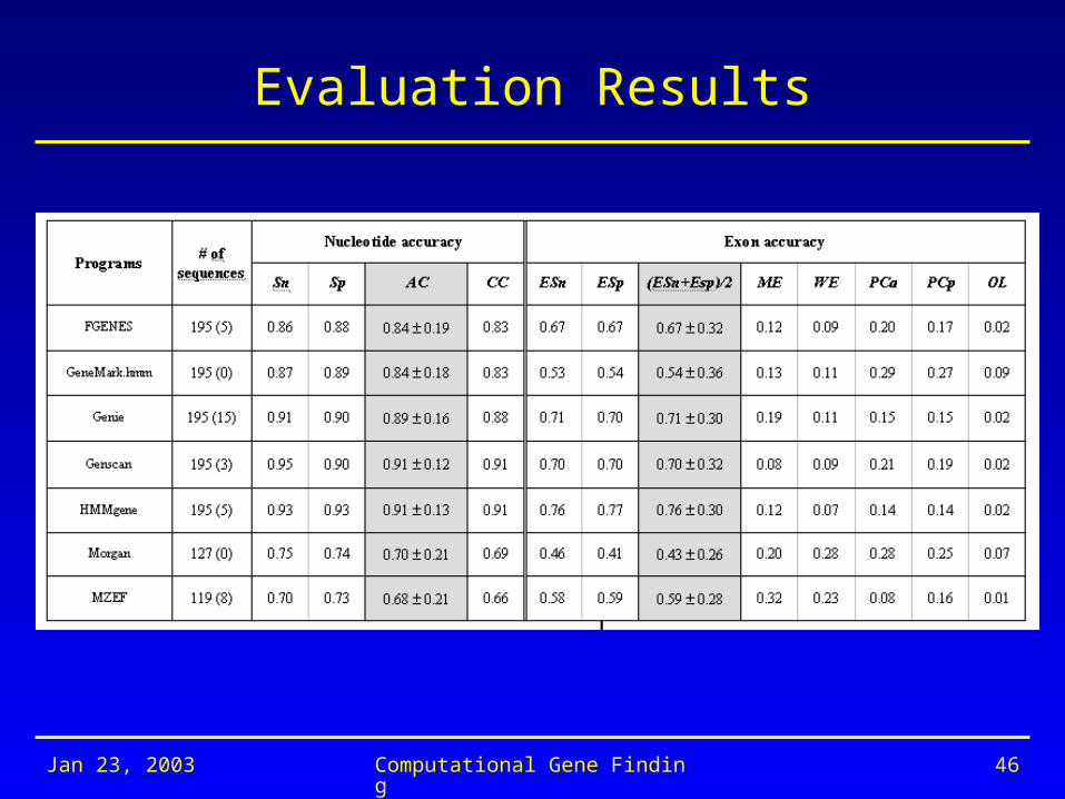
Evaluation in Rogic et al., 2001
• We developed a new dataset for this purposes – HMR195
• Characteristics of the sequences:
– human – mouse – rat origin– Relatively short DNA sequences from GenBank– one gene per sequence– sequences used for the training of the programs were
excluded

Jan 23, 2003 Computational Gene Finding 45
More About HMR195
• Filtering:
– Canonical start and stop codon– No in-frame stop codons– Canonical splice site dinucleotides AG – GT
• Redundancy filtering: similar sequences excluded
• Confirming exon locations using mRNA alignment
Jan 23, 2003 Computational Gene Finding 46
Evaluation Results

Jan 23, 2003 Computational Gene Finding 47
Additional Testing
• Accuracy as a function of sequence and prediction characteristics:
– GC content– exon length– exon type– exon type and signal – exon probabilities and scores– phylogenetic specificity
Jan 23, 2003 Computational Gene Finding 48
Integrated Approaches for Gene Finding
• Programs that integrate results of similarity searches with ab initio techniques (GenomeScan, FGENESH+, Procrustes)
• Programs that use synteny between organisms (ROSETTA, SLAM)
• Integration of programs predicting different elements of a gene (EuGène)
• Combining predictions from several gene finding programs (combination of experts)
Jan 23, 2003 Computational Gene Finding 49
Combining Programs’ Predictions
• Set of methods used and they way they are integrated differs between individual programs
• Different programs often predict different elements of an actual gene
they could complement each other yielding better prediction
Jan 23, 2003 Computational Gene Finding 50
Related Work
• This approach was suggested by several authors
• Burset and Guigó (1996)
– Investigated correlation between 9 gene-finding programs – 99% of exons predicted by all programs were correct– 1% of exons completely missed by all programs
• Murakami and Tagaki (1998)
– Five methods for combining the prediction by 4 gene-finding programs
– Nucleotide level accuracy measures improved by 3-5% in comparison with the best single

Jan 23, 2003 Computational Gene Finding 51
AND and OR Methods
exon 1
exon 2
union
intersection
Jan 23, 2003 Computational Gene Finding 52
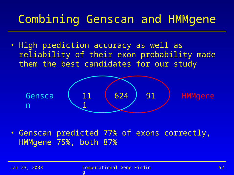
Combining Genscan and HMMgene
• High prediction accuracy as well as reliability of their exon probability made them the best candidates for our study
• Genscan predicted 77% of exons correctly, HMMgene 75%, both 87%
111 624 91Genscan HMMgene

Jan 23, 2003 Computational Gene Finding 53
Control Datasets
• Burset/Guigó dataset – 570 vertebrate genomic sequences containing exactly one multi-exon gene
• Multi-gene dataset – 22 human/murine sequences containing more than one gene
Jan 23, 2003 Computational Gene Finding 54
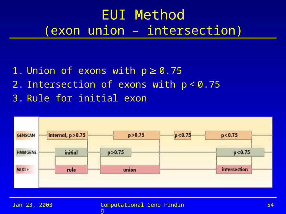
EUI Method(exon union – intersection)
1. Union of exons with p 0.752. Intersection of exons with p < 0.753. Rule for initial exon
Jan 23, 2003 Computational Gene Finding 55
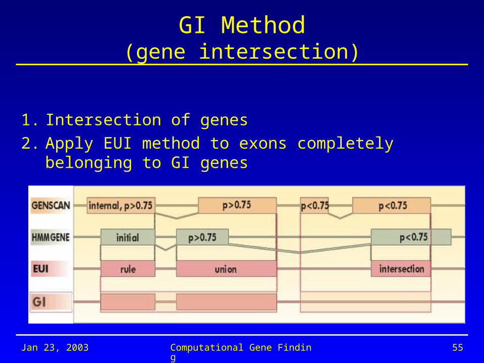
GI Method(gene intersection)
1. Intersection of genes2. Apply EUI method to exons completely belonging
to GI genes
Jan 23, 2003 Computational Gene Finding 56
EUI_frame Method(EUI with reading frame consistency)
1. Assign probabilities to GI genes. Determine position of acceptor and donor site in a reading frame.
2. GI gene with higher probability imposes the reading frame. Choose only EUI exons contained in GI genes that are in a chosen reading frame.

Jan 23, 2003 Computational Gene Finding 57
Results – HMR dataset
• Sp increased 3.2%, ESn increased 2.6%, ESp increased 11.7%• Number of wrong exons significantly decreased
Jan 23, 2003 Computational Gene Finding 58
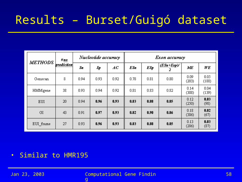
Results – Burset/Guigó dataset
• Similar to HMR195
Jan 23, 2003 Computational Gene Finding 59
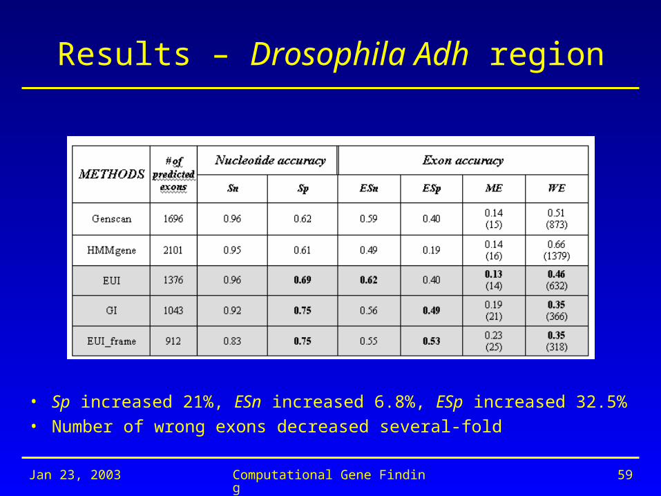
Results – Drosophila Adh region
• Sp increased 21%, ESn increased 6.8%, ESp increased 32.5%• Number of wrong exons decreased several-fold

Jan 23, 2003 Computational Gene Finding 60
Why Does It Work?
Jan 23, 2003 Computational Gene Finding 61
Thank you