jean panaioti jordanou - repositorio.ufsc.br
TRANSCRIPT


Jean Panaioti Jordanou
Echo State Networks for Online Learning Control and MPC of Unknown
Dynamic Systems: Applications in the Control of Oil Wells
Dissertação submetida ao Programa de Pós-graduação em Engenharia de Automação e Sis-temas da Universidade Federal de Santa Catarinapara a obtenção do título de Mestre em Engen-haria de Automação e Sistemas.Orientador: Eduardo CamponogaraCo-orientador: Eric A. Antonelo
Florianópolis
2019

Ficha de identificação da obra elaborada pelo autor, através do Programa de Geração Automática da Biblioteca Universitária da UFSC.
Jordanou, Jean Panaioti Echo State Networks for Offshore OIl and Gas ControlUsing Recurrent Neural Networks: Applications in theControl of Oil Wells / Jean Panaioti Jordanou ;orientador, Eduardo Camponogara, coorientador, EricAntonelo, 2019. 111 p.
Dissertação (mestrado) - Universidade Federal de SantaCatarina, Centro Tecnológico, Programa de Pós-Graduação emEngenharia de Automação e Sistemas, Florianópolis, 2019.
Inclui referências.
1. Engenharia de Automação e Sistemas. 2. Redes deEstado de Eco. 3. Controle Preditivo. 4. Aprendizagem deModelo Inverso. 5. Poços de Produção de Petróleo. I.Camponogara, Eduardo. II. Antonelo, Eric. III.Universidade Federal de Santa Catarina. Programa de PósGraduação em Engenharia de Automação e Sistemas. IV. Título.

Jean Panaioti Jordanou
Echo State Networks for Online Learning Control and MPC of Unknown Dynamic
Systems: Applications in the Control of Oil Wells
O presente trabalho em nível de mestrado foi avaliado e aprovado por banca examinadora
composta pelos seguintes membros:
Prof. Leandro dos Santos Coelho, Dr.
Pontifícia Universidade Católica do Paraná e Universidade Federal do Paraná
Prof. Rodolfo César Costa Flesch, Dr.
Universidade Federal de Santa Catarina
Prof. Gustavo Artur de Andrade, Dr.
Universidade Federal de Santa Catarina
Certificamos que esta é a versão original e final do trabalho de conclusão que foi julgado
adequado para obtenção do título de mestre em Engenharia de Automação e Sistemas
Prof. Werner Kraus Jr., Dr.
Coordenador do Programa
Prof. Eduardo Camponogara, Dr.
Orientador
Florianópolis, 1o de Agosto de 2019.

Este trabalho é dedicado aos meus amigos,
à minha família, e a todos aqueles a quem
este mesmo for útil.

ACKNOWLEDGEMENTS
First, I would like to thank prof. Eduardo Camponogara for all the advising and support,
enabling the development of this work, and also for all the hints in the writing, for the disposition
and patience, and for believing in me. I would also like to thank Eric Antonelo, for all the
advising, support, and enabling me to gather most of the knowledge involved in this work, and
also wisdom on basics such as how to write an academic paper. Further, I would also like to
thank Marco Aurélio Aguiar, for the advising and support, and for helping me with Modelica and
other oil and gas modeling issues. Also, for helping me with the basics of oil and gas industry.
I would like to thank all the people at my research group, for all the support, fun times,
and help regarding the development of my work. Their company was valuable and they gave me
the inspiration and insight necessary for the development of this work.
I would like to thank Ingrid Eidt, for being there and giving me the emotional support I
needed, also for having patience with me and providing me unforgettable moments; my friends
for all the fun moments we had; and my family, due to their support.
Last, but not least, I would like to thank Petrobras, for the funding of this work.

“Perhaps consciousness arises when the
brain’s simulation of the world becomes so
complex that it must include a model of itself.”
(Richard Dawkins, 1976)

RESUMO
Com o avanço da tecnologia, métodos baseados em dados tornaram-se cada vez mais relevantes
tanto na academia quanto na indústria, sendo isso também válido para a área de controle de
processos. Um processo específico que se beneficia de modelagem e controle baseado em dados é
o de produção de petróleo, devido à composição do escoamento multifásico e do reservatório não
serem totalmente conhecidas, assim dificultando a obtenção de um modelo fidedigno. Levando
isso em consideração, neste trabalho há o objetivo de testar e aplicar diversas estratégias de
controle utilizando Redes de Estado de Eco (Echo State Networks, ESN) em modelos de poços
de produção de petróleo. O primeiro controle consiste em usar uma ESN para obter o modelo
inverso online de um processo e usá-lo para computar uma ação de controle de seguimento de
referência. Nesta planta, há dois poços de petróleo com elevação por gás conectados em um riser
por um manifold no qual não há perda de carga. Este primeiro controlador com ESN obteve
êxito em efetuar seguimento de referência em três diferentes combinações de entradas e saídas,
sendo algumas com multiplas variáveis de entrada ou de saída. No segundo método proposto,
utiliza-se uma ESN para servir de modelo numa estratégia de Controle Preditivo Não-linear
Prático (Practical Nonlinear Model Predictive Control, PNMPC), onde obtém-se uma resposta
livre computada de forma não-linear, e uma resposta forçada através da linearização do modelo.
Como a ESN é um modelo analítico, é possível obter facilmente os gradientes para a linearização.
Esse controle ESN-PNMPC efetua seguimento de referência na pressão de fundo de um poço
de petróleo com elevação por gás, também levando em conta restrições operacionais tais como
saturação, limitação de variação, e limites na pressão da cabeça do poço. Este trabalho contribui
à literatura ao mostrar que ambas as estratégias de controle com ESN são efetivas em sistemas
dinâmicos complexos como os modelos de poços de petróleo utilizados, assim como uma prova
de conceito da proposição de utilizar uma ESN no PNMPC.
Palavras-Chave: Redes de Estado de Eco. Controle Preditivo. Aprendizagem de Modelo Inverso.
Poços de Produção de Petróleo.

RESUMO EXPANDIDO
Introdução
Com o avanço da tecnologia, métodos baseados em dados tornaram-se cada vez mais relevantes
tanto na academia quanto na indústria, acompanhando as novas tecnologias tanto de proces-
samento quanto de aquisição de dados. A grande vantagem de se utilizar modelagem baseada
em dados (data-driven) é de não depender do conhecimento da fenomenologia física de um
sistema, visto que os modelos levantados são puramente obtidos pela aquisição de dados. Para
o contexto de controle de processos, abordagens baseadas em dados podem ser benéficas, pois
modelos fenomenológicos estão geralmente sujeitos a incertezas paramétricas e/ou estruturais, ou
podem não ser representativos com relação ao processo a ser controlado. Além disso, utilizando
modelos data-driven pode-se executar o controle de uma planta com o mínimo necessário de
informação prévia. Um dos processos os quais potencialmente se beneficiam de abordagens
baseadas em dados é o de extração de petróleo, devido à composição do escoamento multifásico
e do reservatório não serem totalmente conhecidas, o que aumenta severamente as incertezas
estruturais envolvidas em qualquer modelo fenomenológico, podendo assim resultar em um
modelo pouco representativo do processo. Utilizar metodologias data-driven para controle em
plataformas de petróleo é vantajoso, pois evita a necessidade de saber o tipo exato de escoamento
dentro de um reservatório. A ideia de controle data-driven está intimamente ligada com as
disciplinas de Inteligência Artificial e Aprendizado de Máquina. Nessas áreas de conhecimento,
existem ferramentas convenientes para aplicações de identificação de sistemas e controle, entre
elas as Redes Neurais Recorrentes (RNN), que são modelos simplificados de um cérebro e que
servem principalmente como aproximador universal de sistemas dinâmicos. A desvantagem
de uma RNN está em seu treinamento (Backpropagation Through Time) não ser um problema
de otimização convexo, implicando em mínimos locais e uma aprendizagem mais lenta. Além
disso, há outros problemas como o Vanishing Gradient, que leva um mau condicionamento
numérico devido ao gradiente ser quase nulo em certos pontos. Diversas formas de mitigar essas
desvantagens foram desenvolvidas na literatura, uma delas é através das Redes de Estado de Eco
(Echo State Network, ESN), um subtipo de RNNs onde apenas os pesos de saída são treinados,
mantendo as capacidades de aproximação de uma RNN dado que a parte interna da rede possua a
propriedade de “estado de eco”. Nessas condições, o treinamento da rede passa a ser a resolução
de um problema de mínimos quadrados, possuindo apenas um ótimo global. As redes de estado
de eco são adequadas para aplicações de controle data-driven, seja em Controle Preditivo (MPC),
ou controles onde o modelo precisa ser atualizado online.
Objetivos
Os objetivos gerais desta dissertação incluem montar, aplicar e implementar estratégias de con-
trole data-driven utilizando Redes de Estado de Eco em sistemas de produção de petróleo. A
primeira estratégia, encontrada na literatura, utiliza redes de estado de eco para obter o modelo
inverso online de um processo, utilizando-o para computar uma ação de controle para seguimento

de referência. Esse controle online por modelo inverso é aplicado em um sistema de dois poços
e um riser conectado por um manifold, resolvendo problemas de seguimento de referência e
rejeição de perturbação. O segundo controlador utilizado consiste em um Controle Preditivo
Não-Linear Prático (Practical Nonlinear Model Predictive Control, PNMPC), onde a ESN é
utilizada como modelo de predição. Esse, por sua vez, é aplicado em apenas um poço de petróleo
com elevação por injeção de gás, resolvendo problemas de seguimento de referência.
Metodologia
O controle online por modelo inverso utiliza duas ESNs, uma delas responsável pela obteção de
dados através do algoritmo de Mínimos Quadrados Recursivos (Recursive Least Squares, RLS),
recebendo como saída desejada uma ação de controle aplicada em um instante de tempo no
passado, e como entrada a saída atual e a saída no mesmo instante de tempo da ação de controle
passada; a outra rede é responsável por traduzir os dados obtidos pela rede de treinamento em
ação de controle, tendo como entrada a saída atual e uma saída desejada futura. A rede de treina-
mento transfere a informação através dos pesos que, a partir de um certo valor de saída passada e
ação de controle passada, o valor de saída atual do sistema foi atingido, e com essa informação a
rede de controle deve calcular a ação de controle necessária para colocar o sistema num valor de
saída futura desejado a partir da saída atual. No PNMPC, um modelo não linear é capaz de ser
divido entre uma resposta livre, obtida por simulação do sistema não-linear dado uma ação de
controle mantida no valor corrente, e uma resposta forçada, obtida por aproximação em série
de Taylor com respeito à ação de controle. O método original utiliza o método de diferenças
finitas para calcular o gradiente do modelo, por assumir que o mesmo não está presente ou
é difícil de calcular. Como uma ESN está sendo usada como modelo de predição, a derivada
analítica é facilmente obtida, evitando os problemas de explosão combinatória inerentes no
método de diferenças finitas. Para a implementação dos dois sistemas de controle, é utilizado a
linguagem de programação Python e, no caso do PNMPC, a biblioteca CVXOPT para resolução
dos problemas de otimização quadrática. Os testes se dão por simulações de modelos das plantas
propostas, estes descritos utilizando a linguagem Modelica e interpretados em Python. Para a
primeira aplicação, é utilizado um modelo composicional entre dois poços com elevação via gás
de injeção, um riser e um manifold. O poço é representado por um modelo complexo de ordem
reduzida que utiliza dois volumes de controle, o ânulo, onde se armazena e se transfere o gás
de elevação, e a tubulação, onde se transfere o fluido de produção junto com o gás de elevação.
Possui como condições de contorno a pressão no reservatório, a pressão na cabeça do poço,
e a pressão na entrada do gás de elevação, sendo o poço manipulado através de uma válvula
na entrada de gás e uma válvula choke na cabeça do poço. O modelo do Riser considera dois
volumes de controle, o de uma tubulação horizontal, e o de uma tubulação vertical perpendicular,
onde o fluido é elevado, além de uma válvula no topo referida como “choke de produção”. Suas
condições de contorno são as vazões mássicas de gás e líquido na entrada, e a pressão na saída.
Ambos os modelos possuem comportamento qualitativo similar ao simulador comercial OLGA
(Oil and Gas simulator), e utilizam perda de carga em sua formulação, deixando o sistema

bastante não linear. O manifold conecta a cabeça dos dois poços com a entrada do riser, sem
que a perda de carga seja considerada. Neste trabalho, o controle online por modelo inverso
resolve três problemas de controle distintos relativos a esse sistema: O controle de pressão de
entrada do riser através do choke de produção do mesmo, o controle da pressão de entrada do
riser através das válvulas de gas-lift do poço, e o controle de pressão de fundo de cada poço
utilizando seus respectivos chokes de cabeça. No caso da segunda aplicação, apenas o modelo
de poço com elevação por gás de injeção é utilizado, em um problema que envolve o controle
da pressão de fundo do poço utilizando tanto o choke da cabeça de poço quanto a válvula de
elevação por gás. O controlador também obedece restrições tanto nos valores e nas variações das
variáveis manipuladas, quanto na pressão de topo do poço.
Resultados e Discussões
O controle online por modelo inverso obteve êxito ao efetuar seguimento de referência nas
três tarefas propostas. Nas três configurações de controle propostas, as redes de estado de eco
foram capazes de aprender o modelo inverso do sistema, e o controlador resultante foi capaz
de efetuar o seguimento de referência em cada um dos casos. Também foi efetuada uma busca
de parâmetros em grade para decidir os melhores parâmetros a serem utilizados no controlador
para os três casos, com resultados diversos. Esse controlador se saiu bem em um caso SISO com
uma forte não linearidade no ganho, MISO onde as entradas (válvula de gás de elevação) estão
fisicamente distantes da saída (pressão de entrada do riser), e um caso MIMO onde há um certo
acoplamento entre as variáveis. No caso dos poços, houve também rejeição de perturbação, que
é uma mudança paramétrica no modelo ao longo do tempo, do ponto de vista das ESNs. Para o
controle ESN-PNMPC, ele efetua o seguimento de referência em diferentes pontos de operação,
mesmo com uma pequena discrepância entre o comportamento dinâmico da ESN e do modelo
real do poço. Além disso, o controlador não violou nenhuma das restrições propostas, inclusive
o limite superior na pressão de cabeça do topo, que era medida utilizando as predições da ESN.
Esse seguimento de referência se deu pelo fator de correção da resposta livre, o qual corrige
erros de modelagem e perturbações no sistema.
Considerações Finais
Este trabalho contribui à literatura ao mostrar que ambas as estratégias de controle com ESN são
efetivas em sistemas dinâmicos complexos como os modelos de poços de petróleo utilizados,
assim como uma prova de conceito da proposição de utilizar uma ESN no PNMPC. Levanta
também a ideia de utilizar abordagens data-driven para tais aplicações, que se beneficiam mais
do levantamento de modelos através da obtenção de dados. Como a pesquisa considera mo-
delos simplificados sem ruídos, um trabalho futuro interessante seria aplicar essas metologias
desenvolvidas no contexto de processos reais, para assim avaliar sua tolerância a ruídos e outros
fatores.
Palavras-Chave: Redes de Estado de Eco. Controle Preditivo. Aprendizagem de Modelo Inverso.
Poços de Produção de Petróleo.

ABSTRACT
As technology advances over time, data-driven approaches become more relevant in many
fields of both academia and industry, including process control. One important kind of process
that benefits from data-driven modeling and control is oil and gas production, as the reservoir
conditions and multiphase flow composition are not entirely known and thus hinder the synthesis
of an exact physical model. With that in mind, control strategies utilizing Echo State Networks
(ESN) are applied in an oil and gas production plant model. In the first application, an ESN is
used to obtain online the inverse model of a system where two gas-lifted oil wells and a riser are
connected by a friction-less manifold, and use the resulting model to compute a set-point tracking
control action. Setpoint tracking is successfully performed in three different combinations of
input and output variables for the production system, some multivariate. In the second method,
an ESN is trained to serve as the model for a Practical Nonlinear Model Predictive Control
(PNMPC) framework, whereby the ESN provides the free response by forward simulation and
the forced response by linearization of the nonlinear model. The ESN is an analytical model,
thus the gradients are easily provided for the linearization. The ESN-PNMPC setup succesfully
performs reference tracking of a gas-lifted oil well bottom-hole pressure, while considering
operational constraints such as saturation, rate limiting, and bounds on the well top-side pressure.
This work contributes to the literature by showing that these two ESN-based control strategies
are effective in complex dynamic systems, such as the oil and gas plant models, and also as a
proof of concept for the ESN-PNMPC framework.
Keywords: Echo State Networks. Model Predictive Control. Inverse Model Learning. Oil Pro-
duction Wells.
LIST OF FIGURES
Figure 1 – Plot of an hyperbolic tangent and a sigmoid. . . . . . . . . . . . . . . . . . 41
Figure 2 – Representation of a Feedforward Neural Network with 3 inputs, 2 hidden
layers with 4 neurons each, and 2 outputs. Each arrow represents a weighted
connection between each neuron, represented by a circle. . . . . . . . . . . 42
Figure 3 – Representation of an Echo State Network. Dashed connections (from Reser-
voir to Output Layer) are trainable, while solid connections are fixed and
randomly initialized. . . . . . . . . . . . . . . . . . . . . . . . . . . . . . 47
Figure 4 – Example of a diagram of an offshore production facility. GLM stands for Gas
Lift Manifold. There are two risers and separators due to the fact that one of
the separators is used for testing purposes (JAHN; COOK; GRAHAM, 2008). 49
Figure 5 – Schematic representation of the well considered in this work. . . . . . . . . 51
Figure 6 – Representation of a pipeline-riser system. Pout represents the pressure in the
separator. . . . . . . . . . . . . . . . . . . . . . . . . . . . . . . . . . . . 52
Figure 7 – Representation of a slug flow. . . . . . . . . . . . . . . . . . . . . . . . . . 54
Figure 8 – Schematic of the complete oil and gas production system. . . . . . . . . . . 62
Figure 9 – Block diagram of the ESN-based control framework. Figure extracted from
(JORDANOU et al., 2017). . . . . . . . . . . . . . . . . . . . . . . . . . . 67
Figure 10 – Open loop test of the two wells, one riser system where the riser choke (blue
line) is varied, and both well chokes (red and green line) are fully opened in
a stable and an unstable case, dependent on the gas-lift choke openings . . . 68
Figure 11 – Static curve of the SISO-stable case, where the choke opening z is plotted
against Pin in steady state. Each value of z brings the system to its correpon-
dent value of Pin at the steady state. . . . . . . . . . . . . . . . . . . . . . . 70
Figure 12 – Plot for eT (y axis of topmost plot) and ∆U (y axis of bottom plot) for
different values of δ (x axis). . . . . . . . . . . . . . . . . . . . . . . . . . 74
Figure 13 – Color Grid for eT (a) and ∆U (b) for different values of γ (leak rate, y axis)
and ρ (spectral radius, x axis). Experiment done for the MISO case with the
metrics evaluated during validation and generalization stages (last 4000 time
steps). . . . . . . . . . . . . . . . . . . . . . . . . . . . . . . . . . . . . . 75
Figure 14 – Results for the stable SISO case with z as plant input and Pin as plant output,
where ugs,1 = ugs,2 = 0. The top most plot consists of the controlled variable
Pin (full line), and the desired Pin value (dashed line). The second plot is the
manipulated variable. The third plot gives the mean trajectory error eT over
the 100 previous time steps at each time step. The fourth plot is total control
variation ∆U over the 100 previous time steps, at each time step. . . . . . . 77
Figure 15 – Internal variables related to the Echo State Network and the RLS algorithm.
The first plot consists of the first three terms of a Principal Component
Analysis (PCA) applied over the main diagonal of P[k] over time. The
second and the third plots are the PCA applied to the states of the training
and control ESNs over time. . . . . . . . . . . . . . . . . . . . . . . . . . . 78
Figure 16 – Result for the Anti-Slug Control with the riser choke valve z as manipulated
variable and Pin as controlled variable in an unstable case, where gas-lift
valves are fixed at ugs,1 = 0;ugs,2 = 0.05. The first plot consists on the
controlled variable Pin (full line), and the desired Pin reference value (dashed
line). The second plot is the manipulated variable, the third plot is the mean
trajectory error eT over the 100 previous time steps at each time step, and the
fourth plot is the total control variation over the 100 previous time steps, at
each time step. . . . . . . . . . . . . . . . . . . . . . . . . . . . . . . . . . 79
Figure 17 – Results for MISO control with ugs,1 (blue line) and ugs,2 (green line) as the
plant input and Pin as the plant output, with the riser choke fully open at
z = 1. The first plot consists on the controlled variable Pin (full line), and
the desired Pin value (dashed line). The second plot gives the manipulated
variables, i.e. both gas-lift choke opening. The third plot is the mean trajectory
error eT over the 100 previous time steps at each time step. The fourth plot is
the total control variation over the 100 previous time steps, at each time step. 81
Figure 18 – Result for MIMO control with uch,1 (blue line) and uch2 (green line) as input
and Pbh,1 (blue line) and Pbh,2 (green line) as output. The first plot consists
on the controlled variable Pbh (full line), and the desired Pbh value for both
wells (dashed line). The second plot is the manipulated variables, both gas-lift
choke opening, the third plot is the mean trajectory error eT over the 100
previous time steps at each time step, and the fourth plot is total control
variation over the 100 previous time steps, at each time step. . . . . . . . . . 83
Figure 19 – Result for MIMO control where a disturbance in Pgs,2 is applied, with uch,1
and uch2 as input and Pbh,1 and Pbh,2 as output, where z = 1 and ugs,1 =
ugs,2 = 0.4. The first plot consists on the controlled variable Pin (full line),
and the desired Pbh value for both wells (dashed line). The second plot is the
manipulated variables, both gas-lift choke opening, the third plot is the mean
trajectory error eT over the 100 previous time steps at each time step, and the
fourth plot is total control variation over the 100 previous time steps, at each
time step. The fifth plot represents the step disturbance in the gas-lift source
pressure Pgs,2. . . . . . . . . . . . . . . . . . . . . . . . . . . . . . . . . . 84
Figure 20 – Bottom-hole pressure (Pbh) tracking experiment. . . . . . . . . . . . . . . . 93
Figure 21 – Example of a bidimensional convex set, with a line drawn from an arbitrary
point A to an arbitrary point B, in a generic euclidean space. . . . . . . . . 109
LIST OF TABLES
Table 1 – Parameter values for the oil well . . . . . . . . . . . . . . . . . . . . . . . . 58
Table 2 – Parameter Values for the Experiments. . . . . . . . . . . . . . . . . . . . . . 73
Table 3 – Results for the mean trajectory error, integral absolute error, and maximum
control variation of the stable SISO Pin control manipulating the production
choke z. . . . . . . . . . . . . . . . . . . . . . . . . . . . . . . . . . . . . . 78
Table 4 – Results for the mean trajectory error, integral absolute error, and maximum
control variation of the unstable SISO Pin control manipulating the production
choke z. . . . . . . . . . . . . . . . . . . . . . . . . . . . . . . . . . . . . . 80
Table 5 – Results for the mean trajectory error, integral absolute error and maximum
control variation of the Pin control, manipulating the well gas-lift valves ugs,1
and ugs,2 . . . . . . . . . . . . . . . . . . . . . . . . . . . . . . . . . . . . . 82
Table 6 – Results for the mean trajectory error, integrated absolute error and maximum
control variation of the MIMO coupled wells control, without disturbances. . 83
Table 7 – Results for the mean trajectory error, integral absolute error and maximum
control variation of the MIMO coupled wells control, with disturbances. . . . 83

LIST OF ABBREVIATIONS AND
ACRONYMS
APRBS Amplitude-modulated Pseudo-Random Binary Signal
ARX Autoregressive with Exogenous Inputs
CV Controlled Variables
DMC Dynamic Matrix Control
ESN Echo State Networks
ESP Echo State Property
GPC Generalized Predictive Control
MAC Model Algorithmic Control
MC Memory Capacity
MIMO Multiple Inputs, Multiple Outputs
MPC Model Predictive Control
MV Manipulated Variables
NMPC Nonlinear Model Predictive Control
PNMPC Practical Nonlinear Model Predictive Control
PRBS Pseudo-Random Binary Signal
RLS Recursive Least Squares
RNN Recurrent Neural Network
SISO Single-Input Single-Output
UKF Unscented Kalman Filter
IAE Integral Absolute Error
KKT Karrush-Kuhn-Tucker

LIST OF SYMBOLS
ℓn Refers to the norm n of a vetor.
∞ Infinity.
t Arbitrary instant in time, continous.
k Iteration or discrete time step.
u Input vector of generic state equation system, control action.
x State vector of generic state equation system.
y Output vector of generic state equation system.
x Derivative of x with respect to time.
x(n) nth derivative of x with respect to time.
s Complex variable in the Laplace domain.
K Generic gain.
∑Summation.
x x at an equilibrium point.
θ Generic weights of a linear in the parameters regressor.
∂f(x,y)∂x
Partial derivative of a function f with respect to x.
‖x‖n Norm n of x.
λ Forgetting factor of the Recursive Least Squares algorithm. In chapter 4,
represents friction factors accompanied with subscripts.
Y Prediction vector of a model predictive controller.
∆U Control increment vector of a model predictive controller.
|x| Absolute value of x.
N Normal distribution.
Wtofrom Weight matrices in an Echo State network, where from refers to the variable
the weight matrix pre-multiplies, and to is the output.

f ri Scaling factor of the input weights of the ESN reservoir.
f rb Scaling factor of the bias weights of the ESN reservoir.
ρ Spectral radius of the ESN reservoir weight matrix. In chapter 4, it also
represents densities when indexed.
ψ Sparseness of the ESN reservoir.
γ Leak rate of the ESN.
ω Mass flows in chapter 4.
α Fluid volume fraction in chapter 4.
γ Correction factor of the PNMPC.
δ Time Step Delay prediction in the Online Learning Controller.
eT Mean Trajectory Error.
∆U Total Control Variation (when not bold).
∇x Gradient of vector x.
x∗ Optimum decision variables vector of objective function f(x).
Rn Set of n-th dimensional vectors whose elements are real numbers.
L Lagrangian.
D Lagrangian dual.
λ Equality constraints lagrangian multipliers (when bold).
µ Inequality constraints lagrangian multipliers.

CONTENTS
1 INTRODUCTION . . . . . . . . . . . . . . . . . . . . . . . . . . . . . 20
1.1 Motivation . . . . . . . . . . . . . . . . . . . . . . . . . . . . . . . . . . 20
1.2 Objectives . . . . . . . . . . . . . . . . . . . . . . . . . . . . . . . . . . 23
1.3 Scientific Contributions . . . . . . . . . . . . . . . . . . . . . . . . . . 24
1.4 Organization of the dissertation . . . . . . . . . . . . . . . . . . . . . 24
2 FUNDAMENTALS . . . . . . . . . . . . . . . . . . . . . . . . . . . . . 25
2.1 Dynamical Systems . . . . . . . . . . . . . . . . . . . . . . . . . . . . 25
2.2 System Identification . . . . . . . . . . . . . . . . . . . . . . . . . . . 28
2.2.1 Least Squares Problem . . . . . . . . . . . . . . . . . . . . . . . . . . . 30
2.2.2 Least Squares Analytic Solution . . . . . . . . . . . . . . . . . . . . . . 31
2.2.3 Recursive Least Squares . . . . . . . . . . . . . . . . . . . . . . . . . . 32
2.3 Control Theory . . . . . . . . . . . . . . . . . . . . . . . . . . . . . . . 34
2.3.1 Problem Definition . . . . . . . . . . . . . . . . . . . . . . . . . . . . . . 34
2.3.2 Model Predictive Control . . . . . . . . . . . . . . . . . . . . . . . . . . 35
2.4 Summary . . . . . . . . . . . . . . . . . . . . . . . . . . . . . . . . . . . 39
3 ARTIFICIAL NEURAL NETWORKS . . . . . . . . . . . . . . . . . . 40
3.1 Introduction . . . . . . . . . . . . . . . . . . . . . . . . . . . . . . . . . 40
3.2 Feedforward Neural Networks . . . . . . . . . . . . . . . . . . . . . . 42
3.3 Recurrent Neural Networks . . . . . . . . . . . . . . . . . . . . . . . . 44
3.4 Echo State Networks . . . . . . . . . . . . . . . . . . . . . . . . . . . . 46
3.5 Summary . . . . . . . . . . . . . . . . . . . . . . . . . . . . . . . . . . . 48
4 OIL PRODUCTION SYSTEMS . . . . . . . . . . . . . . . . . . . . . 49
4.1 Offshore Oil Production Systems Overview . . . . . . . . . . . . . . 49
4.1.1 The Wells . . . . . . . . . . . . . . . . . . . . . . . . . . . . . . . . . . . 50
4.1.2 Subsea Processing . . . . . . . . . . . . . . . . . . . . . . . . . . . . . 50
4.1.3 Manifolds . . . . . . . . . . . . . . . . . . . . . . . . . . . . . . . . . . . 50
4.1.4 Pipeline-Riser . . . . . . . . . . . . . . . . . . . . . . . . . . . . . . . . . 51
4.1.5 Separator and Top-side Processing . . . . . . . . . . . . . . . . . . . . 52
4.1.6 Flow Assurance Issues . . . . . . . . . . . . . . . . . . . . . . . . . . . 52
4.1.7 Slugging Flow . . . . . . . . . . . . . . . . . . . . . . . . . . . . . . . . 53
4.2 Well Model . . . . . . . . . . . . . . . . . . . . . . . . . . . . . . . . . . 54
4.3 Riser . . . . . . . . . . . . . . . . . . . . . . . . . . . . . . . . . . . . . . 57
4.4 System Model: Two Wells and one Riser . . . . . . . . . . . . . . . . 61

4.5 Control Applications in Oil Wells and Risers . . . . . . . . . . . . . 62
4.6 Summary . . . . . . . . . . . . . . . . . . . . . . . . . . . . . . . . . . . 65
5 ON-LINE LEARNING CONTROL . . . . . . . . . . . . . . . . . . . . 66
5.1 Description . . . . . . . . . . . . . . . . . . . . . . . . . . . . . . . . . . 66
5.2 Control Challenges . . . . . . . . . . . . . . . . . . . . . . . . . . . . . 67
5.3 Experiments and Results . . . . . . . . . . . . . . . . . . . . . . . . . 69
5.3.1 Implementation . . . . . . . . . . . . . . . . . . . . . . . . . . . . . . . . 70
5.3.2 Metrics and Experimental Setup . . . . . . . . . . . . . . . . . . . . . . 70
5.3.3 On Parameter Selection . . . . . . . . . . . . . . . . . . . . . . . . . . . 72
5.3.4 Riser Inlet Pressure Stable SISO Control . . . . . . . . . . . . . . . . . 76
5.3.5 Anti-Slug Control . . . . . . . . . . . . . . . . . . . . . . . . . . . . . . . 79
5.3.6 Super-Actuated Control . . . . . . . . . . . . . . . . . . . . . . . . . . . 80
5.3.7 Coupled Well Control . . . . . . . . . . . . . . . . . . . . . . . . . . . . 82
5.4 Summary . . . . . . . . . . . . . . . . . . . . . . . . . . . . . . . . . . . 84
6 ECHO STATE NETWORKS FOR PNMPC . . . . . . . . . . . . . . . 86
6.1 Practical Nonlinear Model Predictive Control . . . . . . . . . . . . . 86
6.2 Problem Formulation: Gas-Lifted Oil Well . . . . . . . . . . . . . . . 90
6.3 Results: Gas-lifted Oil Well . . . . . . . . . . . . . . . . . . . . . . . . 91
6.3.1 Identification . . . . . . . . . . . . . . . . . . . . . . . . . . . . . . . . . 92
6.3.2 Tracking Experiment . . . . . . . . . . . . . . . . . . . . . . . . . . . . . 92
6.4 Summary . . . . . . . . . . . . . . . . . . . . . . . . . . . . . . . . . . . 94
7 CONCLUSION . . . . . . . . . . . . . . . . . . . . . . . . . . . . . . 95
BIBLIOGRAPHY . . . . . . . . . . . . . . . . . . . . . . . . . . . . . 97
APPENDIX 102
APPENDIX A – OPTIMIZATION . . . . . . . . . . . . . . . . . . . . 103
A.1 Unconstrained Optimization . . . . . . . . . . . . . . . . . . . . . . . 104
A.2 Unconstrained Optimization Algorithms . . . . . . . . . . . . . . . . 105
A.3 Constrained Optimization . . . . . . . . . . . . . . . . . . . . . . . . . 107
A.4 Convex Optimization Problems . . . . . . . . . . . . . . . . . . . . . 108
A.5 Quadratic Programming . . . . . . . . . . . . . . . . . . . . . . . . . . 110
A.6 Sequential Quadratic Programming . . . . . . . . . . . . . . . . . . 112

20
1 INTRODUCTION
In this section, the dissertation is introduced. Section 1.1 describes the motivation to
this work, Section 1.2 presents to the reader the objectives of this work, Section 1.3 exposes the
scientific contribution of this dissertation, and 1.4 describes the dissertation organization.
1.1 MOTIVATION
Nowadays, model-based control is widely used both in academia and in industry. A
variety of methods in control recquires a process model so that one can design the control law
(CAMACHO; BORDONS, 1999; HOU; WANG, 2013). However, using analytical, physics-
based models is not without drawbacks. For example, a model that has high accuracy is generally
harder to tune a controller for, and obtaining a high-accuracy model tends to be harder than
designing the controller itself. Also, every model-based controller is susceptible to unmodeled
plant behavior during its run time. There are some types of processes with variables that are
difficult to model exactly, such as an oil and gas reservoir (JAHN; COOK; GRAHAM, 2008).
Another problem is that plants tend to change their behavior over time (e.g. aircraft-related
control), which is difficult to incorporate in a model (HOU; WANG, 2013). Industrial plants
become ever more complex with the progression of years (e. g. industry transition to 4.0),
which hinders the application of model-based control since the synthesis of a model becomes
increasingly difficult. With the recent advances in technology, an alternative is data-driven
modeling and control.
As information science and technology is becoming more developed along the years,
devices are being deployed to collect data in real time from diverse plants such as chemical
processses, metallurgy, machinery, electronics, electricity and transportation (HOU; WANG,
2013). Therefore, it is now even more viable to use data for control design, hence the rise
of Data-Driven Control. Data-driven control has various definitions (HOU; WANG, 2013),
however they more or less include the fact that a controller is designed based on input/output
data information, and no physical information is used. The implementation of data-driven control
should be considered when (HOU; WANG, 2013):
• The model is unavailable;
• The uncertainties involved in the model are difficult to express mathematically;
• The process is difficult to model;
• The possible models are too complex in terms of number of variables, parameters and
algebraic equations for control design.
Chapter 1. Introduction 21
Data-driven control is closely related to artificial intelligence and machine learning
(HOU; WANG, 2013; BISHOP, 2006) and black-box system identification (NELLES, 2001),
which seek to obtain a model purely from input-output data. Science and technology in those
fields have advanced significantly in recent years as a result of industrial and academic research,
and many machine learning and system identification methods and tools were developed along
the years. One of such tools from the fields of artificial intelligence and machine learning is the
Recurrent Neural Network (RNN) (GOODFELLOW; BENGIO; COURVILLE, 2016), which
is widely used as universal approximators for nonlinear systems. When given a sufficiently
representative training set, RNNs can reproduce the behavior of a wide variety of nonlinear
plants. However, one issue with these networks is that they tend to be hard to train, for being a
nonlinear model on the training parameters, and complex algorithms such as the backpropagation
through time (BPTT) have to be used for their parameter tuning. Also, due to its nonlinearity,
local optima abound. For data-driven control applications, a learning model that is simpler to
train can ease the calculation of the control law. In the specific case of a system that has least
squares training, one can apply fast-convergent online algorithms such as the Recursive Least
Squares (RLS) for adaptive control.
One possible solution that retains the abstraction power of the RNNs while being simple
to train is the Echo State Network (ESN) (JAEGER et al., 2007). The ESN is basically an RNN
where only the state-output weights are trained, and the recurrent layer of the network provides a
rich variety of dynamical behavior which the output is a linear combination of. For this very rea-
son, the set of all the neurons in the recurrent layer of the network is referred to as the “reservoir”,
and they are connected to each other by fixed weights that are randomly initialized. Because the
relation between the neurons in the recurrent layer and the neurons in the output layer is linear,
the Least Squares algorithm can be used to train an ESN. Meanwhile, the fixed dynamic reservoir
provides a large pool of dynamics to the ESN when there is a sufficiently large number of neurons
in it. The state-output Least Squares training is effective as long as the reservoir has the “echo
state property” (JAEGER, 2001), which will be explored further in this work. Some examples
of successful uses of Echo State Networks are: learning complex goal-directed robot behaviors
(ANTONELO; SCHRAUWEN, 2015), grammatical structure processing (HINAUT; DOMINEY,
2012), short-term stock prediction (technical analysis) (LIN; YANG; SONG, 2009), predic-
tive control (PAN; WANG, 2012; XIANG et al., 2016), wind speed and direction forecasting
(CHITSAZAN; FADALI; TRZYNADLOWSKI, 2019), blast furnace gas production forecasting
(MATINO et al., 2019), and noninvasive fetal detection (LUKOŠEVICIUS; MAROZAS, 2014).
In oil and gas, ESNs have shown promising results in identifying the complex dynamics involving
a slugging flow riser (ANTONELO; CAMPONOGARA; FOSS, 2017), which is considered
a difficult task in system identification. Also, the ESN has outperformed wavelet networks in
autonomous vehicle applications (KHODABANDEHLOU; FADALI, 2017) There are also works
proposing methods to treat noise in Echo State Networks, such as (XU; HAN; LIN, 2018), which
use the ESN alongside the wavelet denoising algorithm.
Chapter 1. Introduction 22
Echo State Networks are convenient for online control because of its linear training. Since
the ESN can be trained with Least Squares, then RLS can also be deployed. A remarkable use of
ESN in on-line learning control is applied by (WAEGEMAN; WYFFELS; SCHRAUWEN, 2012),
where an ESN is trained online by RLS to obtain a process inverse model and use this model to
directly calculate the control action. In (WAEGEMAN; WYFFELS; SCHRAUWEN, 2012), a
variable delay heating tank, a steady cruise plane and an inverted pendulum model are used to
test the methodology. The strategy presented in (WAEGEMAN; WYFFELS; SCHRAUWEN,
2012) was also used for an industrial hydraulic excavator (JAHN; COOK; GRAHAM, 2008), and
expanded and used in a robotic manipulator (WAEGEMAN; HERMANS; SCHRAUWEN, 2013).
Another work applying ESN for online learning control is (BO; ZHANG, 2018), where they are
used in a reinforcement learning actor-critic framework where each ESN performs training online
to solve a dynamic programming problem for wastewater treatment. The controller developed
in (WAEGEMAN; WYFFELS; SCHRAUWEN, 2012) is referred to as the “Online Learning
Controller” for the rest of this work. Another work (CHOI et al., 2017) also utilizes the ESN as an
inverse model for control. The application is a lower extremity exoskeleton, however the training
is applied offline. An example of the use of a trained online ESN for system identification is
the work of (YAO; WANG; ZHANG, 2019), where a variation of the ESN for online learning
is presented and a different algorithm is proposed based on the new structure. Another work
which deals with time series prediction and system identification using ESNs is (YANG et al.,
2019), where a variation of the RLS is proposed that outperforms de regular one. The proposed
variation includes ℓ0 and ℓ1 norm into the RLS formulation and boosts the algorithm performance
significantly. There are, however, other alternatives to boost performance in a RLS algorithm
applied to an ESN, such as (ZHOU et al., 2018), where a kernel is incorporated to the readout
layer of the ESN.
Another control field that benefits from Echo State Networks is Nonlinear Model Pre-
dictive Control (NMPC). There are works in the literature combining Echo State Networks and
MPC, such as (PAN; WANG, 2012; XIANG et al., 2016; HUANG et al., 2016). The first, (PAN;
WANG, 2012), uses state space per time step linearization to compute the control action, however
the model-plant correction is done using a time-variant parameter and without integration. The
second, (XIANG et al., 2016), does only one linearization of the ESN at a certain operating point.
The third, (HUANG et al., 2016), utilizes an online-trained Echo State Network as a predictor for
the control of a pneumatic muscle. The controller itself is a single-layered feedforward neural
network trained by particle swarm optimization. The proposal of this work is to use the ESN
together with the PNMPC (Practical Nonlinear Model Predictive Control, (PLUCÊNIO et al.,
2007)) strategy. The PNMPC performs only input linearization to separate the response into a
free and a forced response, and uses a filtered integral error as model correction factor. The only
issue is that, since PNMPC assumes that the model derivative is not possible to obtain, it uses
Finite Differences to calculate the gradients for linearization, which hinders its performance due
to combinatorial explosion. The advantage of using an Echo State Network in this context is that

Chapter 1. Introduction 23
since a clear analytical model is present, the gradients are easier to obtain. Also, the ESNs are
powerful identification tools, hence the idea to use an ESN as the prediction model for PNMPC.
An application that would benefit from the types of data-driven controllers described are
dynamic oil production related applications. More specifically, applications related to Flow Assur-
ance (JAHANSHAHI, 2013), which aims to maintain flow integrity in the oil and gas produced.
In the literature, there are many solutions to flow assurance problems that use model-based feed-
back control, such as (JAHANSHAHI, 2013), (OLIVEIRA; JÄSCHKE; SKOGESTAD, 2015),
(CAMPOS et al., 2015), and (STASIAK; PAGANO; PLUCENIO, 2012). Since in model-based
control one has to specifically model the flow that is being produced inside the production system,
a lot of uncertainties are present since the flow nature is not generally known (JAHANSHAHI,
2013). It is then proposed the use of data-driven control in Oil and Gas applications, as the exact
flow may not be known.
Both tasks include the Echo State Network in the form of parallel system identification
(NELLES, 2001) and as such, the ESNs do not receive direct information of the processes
previous outputs (control actions, in terms of the online learning controller), only calculating the
network output by using the previous inputs.
1.2 OBJECTIVES
In this work, the main objective is to apply the Online Learning Controller (WAEGE-
MAN; WYFFELS; SCHRAUWEN, 2012) and the proposed ESN-based PNMPC into the context
of Oil and Gas production systems. For that end, experiments are performed applying these two
controllers into reduced-order models of oil and gas production platform components. All the
models used were compared to OLGA (Oil and Gas Simulator) and deemed sufficiently accurate
(JAHANSHAHI; SKOGESTAD, 2011; JAHANSHAHI; SKOGESTAD; HANSEN, 2012).
This work consists into these two main applications:
• Application of the Online-Learning Control (WAEGEMAN; WYFFELS; SCHRAUWEN,
2012) into a system containing two gas-lifted oil wells, whose models are developed by
Jahanshahi et al. (JAHANSHAHI; SKOGESTAD; HANSEN, 2012), and one riser, whose
model was conceived by Jahanshahi and Skogestad (JAHANSHAHI; SKOGESTAD, 2011).
These components are connected by a manifold where no pressure drop due to friction is
present. The Online Learning Controller is simulated with the resulting system using three
different input-output configurations.
• Application of the ESN-PNMPC framework into a single gas-lifted oil well model, from
(JAHANSHAHI; SKOGESTAD; HANSEN, 2012). The controller has the objective to
follow bottom-hole pressure setpoints while avoiding constraints relatated to the top-side
pressure, by using both the gas-lift choke and the top-side production choke.
Chapter 1. Introduction 24
In the end, by succesfully applying these two ESN-based controllers into oil and gas
production plaftorm problems, it is shown the viability of data-driven methods for control and
proxy modeling in these fields.
1.3 SCIENTIFIC CONTRIBUTIONS
The work in this dissertation has also contributed to the literature in the form of:
• Publication in the Proceedings of the Brazilian Symposium on Intelligent Automation
(SBAI), 2017 (JORDANOU et al., 2017).
• Publication in the Proceedings of the 3rd IFAC Workshop on Automatic Control in
Offshore Oil and Gas Production (OOGP), 2018 (JORDANOU et al., 2018).
• Paper published in the journal “Engineering Applications of Artificial Intelligence” (JOR-
DANOU; ANTONELO; CAMPONOGARA, 2019).
1.4 ORGANIZATION OF THE DISSERTATION
The remainder of this dissertation is organized as follows:
• Chapter 2 describes the fundamental concepts to better understand this research work,
such as optimization, dynamic systems, system identification and control theory.
• Chapter 3 describes Artificial Neural Networks, going from Feedforward NNs to Echo
State Networks.
• Chapter 4 explains oil and gas platforms, and also shows the models used to describe a
gas-lifted oil well and a pipeline-riser system.
• Chapter 5 introduces the reader to the Online-Learning Control Strategy, while reporting
experiments on its application to a system of two wells and one riser, connected by a
manifold.
• Chapter 6 describes the strategy developed in this work, the ESN-based Practical Nonlinear
Model Predictive Control (ESN-PNMPC). Also, the chapter under consideration shows
experiments of the application of the ESN-PNMPC to a single gas-lift oil well.
• Chapter 7 then concludes this dissertation.
25
2 FUNDAMENTALS
This Chapter discusses fundamental concepts, found in literature, essential for the under-
standing of this work. It goes through:
• Dynamic Systems (Section 2.1);
• System Identification (Section 2.2); and
• Control Theory (Section 2.3).
These are the three pillars for the development of this work. If the reader is familiar with the
theories mentioned, then this chapter can be skipped without further compromising reading. It
is assumed that the reader has a small familiarity with multivariate and vector calculus, linear
differential equation solutions and linear algebra. Some of these theory utilize optimization in
the background. A brief review on optimization models and algorithms appear in Appendix A.
2.1 DYNAMICAL SYSTEMS
A system is defined as a relation between an input and an output, where an unique output
response is generated by the input (CHEN, 1998). A dynamical system is a system that depends
not only on current input, but also on past inputs (CHEN, 1998).
Generally, a dynamical system response at the current time t depends on all inputs applied
from time −∞ to t. To avoid computing that, which is impractical if not impossible, either a
differential equation representation (input-output representation) or state equations representation
is used.
A state is a variable that, when paired up with the input, defines uniquely the value of the
output (CHEN, 1998). The state depends on the current input and recursively on itself, so it is a
representation of all the inputs applied to the system from time −∞ to t.
In practice, inputs are variables which can be manipulated directly, such as the opening
of a tank valve or the steering wheel of a car. Outputs are the data that can be gathered by human
beings or instruments, such as the speed-reading pointer at a car or a temperature measurement
from a thermometer.
Memory (the dependence on past information) is what defines a dynamical system, but a
system can have other classifications regarding a few properties:
• Causal or non-causal: A causal system does not depend on future inputs to compute the
output. All physical dynamical systems are causal (CHEN, 1998).

Chapter 2. Fundamentals 26
• Continuous-time or discrete-time: A continuous-time (discrete-time) system has its
input, state and output signals in continuous-time (discrete-time). A discrete-time signal
is a signal that, when computed from −∞ to ∞, has an infinite but countable number of
values. When a continous-time signal is computed on a small interval [t, t+ δ], with δ in
this case being an arbirarily small number, it has infinitely uncountable points.
• Linear or non-linear: A function f is linear, if and only if αf(x)+βf(y) = f(αx+βy),
for any arbitrary (α,β,x or y). This is analogue to systems. Several mathematical tools are
avaiable in the literature, such as in (CHEN, 1998), to deal with linear systems. The systems
used for this work, along with almost all physical systems in the real world, are always
non-linear. When the non-linearity is weak, a non-linear system can be approximated
locally by a linear system. These approximations are used to define stability properties of
a nonlinear system, as seen below.
• Time-variant or time-invariant: If a system is time-invariant, its behavior will never
change over time. As with linearity, this assumption can also facilitate calculations, but
systems tend to have time-variance, which is ignorable or not, depending on how slow the
effect is. A slow time variant parameter such as the pressure in a oil and gas reservoir can
be considered to be time-invariant for control purposes.
It is difficult to find an exact mathematical representation of a real life system. This
limitation is circunvented through the use of models. A model is a less complex, easier to
understand approximation of the real world system. The model’s complexity is directly related
to its precision. The more complex a model is, the harder its computing becomes, so it is ideal to
specify the model as simple as an application needs it to be.
There are several ways to represent a dynamic system by models. If the model is
continuous and non-linear, it can be represented as an O.D.E (Ordinary Differential Equation),
as follows:
f(y(t), y(t)...,y(n)(t)) = g(u(t), u(t), ....u(n)(t)) (2.1)
where y(t) is the output vector and u(t) is the input vector. For a generic function x(t), x(t) is
defined as the 1st derivative of x in time. x(n)(t) is defined as the n-th derivative of x in time. Or
it can be represented as a system of first order ODEs, called state equations:
x(t) = f(x(t),u(t)) (2.2)
y(t) = g(x(t),u(t)) (2.3)
with x(t) being the state vector at time t.
In case the model is in discrete time, the model can be represented by n-th order difference
equations:
f(y[k],y[k − 1], ...,y[k − n]) = g(u[k],u[k − 1], ...,u[k − n]) (2.4)

Chapter 2. Fundamentals 27
or by a system of n first order difference equations:
x[k + 1] = f(x[k],u[k]) (2.5)
y[k] = g(x[k],u[k]) (2.6)
If a system is linear, there are additional representations for the system, such as:
• Transfer Function: An input-output representation described by the Impulse Response of
the system in the Laplace domain. The impulse response is the response of the system to
an impulse-type excitation (CHEN, 1998). It is easily obtainable by applying the Laplace
transform into a differential equation representation of the system and assuming null state
(initial condition 0 for the differential equation). Generally has the following form:
Y (s)
U(s)=B(s)
A(s)(2.7)
where Y (s) is the Laplace transform of the output and U(s) is the Laplace transform of
the input. As this transform can draw information on the system response for a sinusoidal
signal at any given frequency, the Laplace transform of a system is also referred to as
the Frequency Domain. The roots for the polynomial A(s) are referred to as poles, and
contain relevant information about the dynamical response of the system, such as the
transient speed, and oscillations. The roots for the polynomial B(s) are the zeroes, which
also provide information of the system response. When s = 0, the steady state gain K of
the system can be obtained. Exciting the system with a unitary step input will bring its
output to K at steady state. As the transfer function representation is simple, and easy to
deal with algebraically because of the Laplace transform properties, it is widely used in
the context of control theory. An ARX (Autoregressive with Exogenous Output) model
(NELLES, 2001) can also be seen as a discrete-time transfer function, providing enough
information about the identified system behavior.
• State-Space Representation: If a system is linear, it is represented only by a linear combi-
nation of the system states and inputs. Thus, it is possible to obtain a matrix representation
of the system. A state space system has the following structure:
x = Ax + Bu (2.8)
y = Cx + Du (2.9)
where x is the state vector, u is the input vector, and y is the output vector. The Eigenvalues
of A provide information on the system dynamics the same way as the poles of a transfer
function. In fact, a transfer function can be converted to state-space form. This conversion
is referred to as the realization of a system (CHEN, 1998). A transfer function has infinite
state-space realizations. It is also possible to obtain the information whether the system

Chapter 2. Fundamentals 28
is controllable or not through matrices A and B, and observable through A and C. In a
rough definition, a system is controllable if the state can be set to any value by an arbitrary
input, and a system is observable if every system state can be obtained given the output.
The state-space representation is a more general representation of the system, providing
information of the system, and it is widely used in robust control and optimal control
applications (MACKENROTH, 2013).
An important concept related to non-linear systems is the equilibrium point, which for
continuous systems is a state vector x that satisfies the following condition:
0 = f(x,u) (2.10)
whereby x = 0 means that the state is constant over time. Equilibrium points can be stable or
unstable. This is easily analyzed if the eigenvalues of the Jacobian of f(·) are all nonzero and
finite. The Jacobian is utilized to linearize the system in the neighborhood of the operating points.
If one of the Jacobian’s Eigenvalue is either zero or infinite, the linearized system’s behavior
does not represent the nonlinear system.
An equilibrium point being stable means that, for any state at an instant t, x(t) = x+ δ,
with δ being a vector of sufficiently small numbers, the dynamic system state will converge to x
at t → ∞. An unstable equilibrium point has the opposite behavior. Any x(t) = x + δ for small
δ will diverge from x.
2.2 SYSTEM IDENTIFICATION
As explained in Section 2.1, there is a difference between a mathematical model and a
real-life system. A model is almost always a simpler approximation of a system which is present
in real life.
When reffering to a real-life application, three levels of prior knowledge of a certain
physical system are considered in the literature (NELLES, 2001):
• White-Box Model: Sufficient information of the physical phenomena involved in the
system modeling is known. Requires identification of very few, if any, parameters.
• Grey-Box Model: A certain amount of information about the system is known. Some
dynamics are unknown or too hard to model, needing identification.
• Black-Box Model: No prior knowledge of system is avaiable or it is too hard to model.
The identification problem extends for all dynamics of interest in the desired application.
System identification consists in using data driven information so as to find a model that
behaves the closest possible to the real-life system in a certain operating region. Ideally, it would
Chapter 2. Fundamentals 29
be desirable that the model behaves just like the system in all possible regions of operation but,
if that task is not impossible, its difficulty is impracticably high and the model would have to be
too complex to be tractable. A simple model would be easier to control and/or optimizing.
There are two ways to gather data for model identification: online or offline. A model is
identified offline when all the data is given at once, from a separate runtime of the process. The
model is identified online when data is given to the model and the model is validated all at the
same time the data is output by the plant.
According to (NELLES, 2001), a system identification problem consists in these eight
steps:
1. Choice of Model Inputs: In a control context, usually the inputs of an identified model
are all the manipulated variables available.
2. Choice of Excitation Signal: The excitation signal in a linear system is easily defined by
a Pseudo Random Binary Signal (PRBS), due to this signal class having a well defined
frequency spectra, even though being pseudo-random in the time domain. For a non-linear
system, this choice is nontrivial, due to the fact that a PRBS takes advantage of the constant
input-output gain of a linear system, which does not happen on a non-linear system. In
(NELLES, 2001), there is an introdution to the vast theory that is nonlinear system
excitation for identification. A common example of signal utilized in nonlinear system
identification is the APRBS (Amplitude-modulated Pseudo-Random Binary Signal), which
is merely the PRBS, but varying in amplitude as well.
3. Choice of Model Architecture: The model architecture depends on the intended use, the
problem type, the problem dimensionality, the avaiable amount of data, time constraint,
memory restrictions, or if the model is learned online and offline.
4. Choice of Dynamics Representation: Problem dependent, since it consists of which
variables will be used to represent the dynamics of the system.
5. Choice of Model Order: Trial and error by grid-search could be applied, however in the
literature (NELLES, 2001) there are several methods available. For instance, the forward
selection, where the search starts from the lowest order model and the order rises until
there is no more gain in performance.
6. Choice of a Model Structure: Trial and error by grid-search could be applied, but there
are more sophisticated methods available in the literature (NELLES, 2001). For instance,
(BILLINGS, 2013) present a strategy utilizing Orthogonal Least Squares (OLS) in the
context of selecting a structure for a NARMAX (Nonlinear Autoregressive Moving-
Average with exogenous output) model. Criteria such as the Error Reduction Ration
(BILLINGS, 2013) can be used to define the ideal structure in a NARMAX model.

Chapter 2. Fundamentals 30
7. Choice of Model Parameters: Generally the parameter choice can be reduced to opti-
mization problems. If the parameters are linear, then the optimization problem that is
solved is a linear least squares problem. The fitting of the model is also called “training”,
and the data used for fitting is called “training data”.
8. Model Validation: The criteria to evaluate a certain model’s performance is application-
dependent. The easiest metric to evaluate performance is the training error of the model,
which is the error between the system and the model, evaluated at the training points
(NELLES, 2001). A model not having low enough training error is called “underfitting”,
which means that the model is not complex enough to fit the data and a more intricate
model should be chosen. The opposite of underfitting would be “overfitting”, when the
model is too complex and can fit almost perfectly the training data, but it is not capable of
generalization. In other words, it has high “test error”, error of approximating acquired
data which are not used for fitting the model. Both problems are structural by nature, but
could be solved by regularization (BISHOP, 2006).
The higher a model order and the more complex a structure, the higher the capacity of
fitting the data. High complexity models can lead to overfitting problems, which can be avoided
through grid search and cross-validation strategies for parameter decision (NELLES, 2001;
BISHOP, 2006).
2.2.1 Least Squares Problem
The least squares problem is ubiquous in linear system identification problems. The
objective is to minimize the following cost function:
J =N∑
k=0
‖y[k] − y[k]‖22 (2.11)
This cost function represents the quadratic error between the identification model’s
estimated output y[k] and the real output y[k] at time k, for the N samples. Here, it is assumed
that both y[k] and y[k] are scalars. However, in case of a multi-output identification problem, this
problem is solved for each output. The model can be described, for instance, as y[k] = θT x[k].
The linear parameter vector θ is the decision variable in this problem and is multiplied by the
input vector x[k], which contains all features that are used to describe a model (e.g., x[k] =
(u[k], y[k], y[k − 1])T , with u[k] being an input to the system and y[k],y[k − 1] being two values
of the output at different instants of time).
Since the cost function is quadratic and the model is linear, it has one global minimum
that can be analytically found if devoid of constraints. This implies that there is a value for θ that
brings y[k] as close as possible to y[k].

Chapter 2. Fundamentals 31
In matrix form, J is represented as:
J = (Xθ − Y)T (Xθ − Y) (2.12)
with X being evaluated as xT [k] in line k and Y is defined as the vector that the element at
line k equals to y[k]. If a symmetric, positive definite weight matrix Q is added in a way that J
becomes:
J = (Xθ − Y)T Q(Xθ − Y) (2.13)
This version of the problem is known as “Weighted Least Squares”. Since a row belonging
to matrices X and Y represents the sample collected at time k in a system identification training
process, the importance of each observation at time k can be scaled. This is actually used in the
Recursive Least Squares algorithm.
The Least Squares Problem applies not only to purely linear functions, but to functions
which are linear in the parameters, such as an Echo State Network or any n-degree polynomial.
All it needs to be done is treating the non-linear terms multiplying the linear parameters as new,
separate inputs (NELLES, 2001). (e.g., to fit a model θ1u2 + θ2u+ θ3, all it needs to be done is
letting x[k] be (u[k], u2[k], 1)T in the point of view of the cost function).
As mentioned in section 2.2, a model which has a large number of parameters can
perform better at the minimization of the “training error”, which is the error that this problem is
trying to minimize, but will not be able to fit points outside the training region. One way to work
around this problem is with the Tikhonov regularization (ANTONELO; CAMPONOGARA;
FOSS, 2017), (NELLES, 2001), which consists in penalizing the magnitude of the decision
variables. This boosts the capacity of a model to generalize and is easier than optimizing the
model structurally (NELLES, 2001). Adding regularization, the cost function would be:
J = (Xθ − Y)T (Xθ − Y) + βθT θ (2.14)
with β being a scalar whose purpose is to penalize the ℓ2-norm of θ.
2.2.2 Least Squares Analytic Solution
The derivation to the solution of the Least Squares Problem is in (NELLES, 2001). To
analytically solve a convex problem, θ must satisfy ∂J(θ)∂θ
= 0. Since J is quadratic, this implies
solving a linear system. Below is the solution to the three versions of the least squares problem
presented:
Least Squares:
θ = (XT X)−1XT Y (2.15)

Chapter 2. Fundamentals 32
Weighted Least Squares:
θ = (XT QX)−1XT QY (2.16)
Regularized Least Squares (Also known as Ridge Regression):
θ = (XT X + βI)−1XT Y (2.17)
where I is the identity matrix.
The inverse shown in the solution of all the Least Squares version is not actually computed
in a numerical least squares solver. A cheaper way to compute the solution is to find θ as a
solution to the following linear system:
XT Xθ = XT Y (2.18)
This way, the computation of the inverse matrix of XT X is avoided.
2.2.3 Recursive Least Squares
The derivation of the Recursive Least Squares (RLS) form the Analytic Solution of the
Least Squares problem is in (NELLES, 2001). This version of the Recursive Least Squares is
derived from a Weighted Least Squares Problem where:
Q =
λn 0 · · · 0
0 λn−1 · · · 0...
.... . .
...
0 0 · · · λ0
(2.19)
and λ is called the forgetting factor which is generally 0.9 ≤ λ ≤ 1 (NELLES, 2001). If λ = 1,
then Q would be the identity matrix, so it would be equivalent to a normal Least Squares problem.
λ is called the forgetting factor due to the fact that, if λ < 1, and assuming each training example
corresponds to a time step in a simulation or the sample time of a generic data acquisition system,
then the quadratic error of recent samples receives more consideration during optimization. The
result would then perform better for these selected points. In a sense, the optimizer is “forgetting”
older samples.
Another way to represent the Weighted Least Squares cost function is:
J =N∑
k=0
λN−k‖y[k] − y[k]‖22 (2.20)

Chapter 2. Fundamentals 33
To derive the least squares problem for the Recursive Least Squares algorithm, some
auxiliary definitions are recursively made:
X[k + 1] =
X[k]
xT [k + 1]
(2.21)
Y[k + 1] =
Y[k]
y[k + 1]
(2.22)
Y[0] = y[0] (2.23)
X[0] = xT [0] (2.24)
Naturally, the value of θ at time step k must be defined, which would be:
θ[k] = (XT [k]QX[k])−1XT [k]QY[k] (2.25)
θ[k + 1] = (XT [k + 1]QX[k + 1])−1XT [k + 1]QY[k + 1] (2.26)
Then, the following definition is applied:
P[k] = (XT [k]QX[k])−1 (2.27)
which is known as the correlation matrix and carries all the runtime information that the system
has learned. Due to it being defined as the inverse of XT X, the computation of an inverse matrix
is avoided.
Using these definitions, a way to compute θ[k] from θ[k − 1] is derived from (NELLES,
2001), as follows:
P[0] =1
αI (2.28)
e[k] = θT [k − 1]x[k] − y[k] (2.29)
P[k] =P[k − 1]
λ− P[k − 1]x[k]xT [k]P[k − 1]
λ(λ+ xT [k]P[k − 1]x[k])(2.30)
θ[k] = θ[k − 1] − e[k]P[k]x[k] (2.31)
The e[k] is called the “a priori error”, since it computes the error using θ[k − 1] (the
parameters of the previous iteration’s model).
The α is the “learning rate”. If a priori data for the system is already provided, then P[0]
could be (XT QX)−1 with X being the data already gathered about the system. If not, P[0] is,
for simplicity purposes the identity matrix multiplied by 1α
. The smaller the parameter α is, the
more it is assumed that the system is unknown to the algorithm. It would be ideal that α = 0.01
or α = 0.001 (NELLES, 2001), for leading to high corrections on the error.

Chapter 2. Fundamentals 34
2.3 CONTROL THEORY
This section gives a brief introduction of control theory. Control theory is ubiquous in
techonology, such as industrial processess, robotics, and even household appliances such as an
air conditioner. To control is to bring a certain set of variables (referred to as controlled variables
(CV)) to a certain value (called the setpoint), by using a manipulated variable (MV) that one can
directly define the value, such as a valve opening, a regulated voltage source, or a car’s brake
and accelerator.
In this work, system identification and neural networks theory is used to control an oil
and gas production plant with no prior information.
2.3.1 Problem Definition
A control problem is: given a certain dynamical system with input u(t), state x(t) and
output y(t), and a desired output trajectory y(t), what input trajectory should be applied so that
y(t) = y(t)? The set of rules defining u(t) is also referred to as “control law”, and a “control
strategy” is a structure from which the control law is derived from.
There are two main types of control strategies:
• Feedforward control: No information from the output y(t) is used to compute the control
action. Also called “open-loop” control.
• Feedback control: Information from the output is used to compute the control action.
Also called “closed-loop” control.
Generally in industry, y(t) is a constant signal. In this case, the control problem is about
maintaining a dynamical system (also called a plant) at a certain operation point.
“Open-loop” control could be applied, but if the dynamical system suffers some slight
parametric change, it would deviate further from the setpoint. Even with this change, called
“disturbance”, the setpoint could be determined if the closed-loop control strategy has certain
properties. For more information, refer to (CHEN, 1998). There are two main subtypes of control
problems:
• Setpoint Tracking: Assuming that the system’s output is not y(t), could the system be
brought into the operating point so that y(t) = y(t)? If so, how fast?
• Disturbance Rejection: Assuming that the the system output y(t) is y(t) = y(t), if a
parametric change in the model occurs, could y(t) still equal y(t) at steady state? How
quick would the system come back to its current setpoint?
When a control problem has only one manipulated variable and one controlled variable,
it is called a Single Input, Single Output (SISO) Control Problem. When it has multiple
Chapter 2. Fundamentals 35
variables involved, the control problem is referred to as a Multi Input, Multi Output (MIMO)
problem.
2.3.2 Model Predictive Control
Model Predictive Control (MPC) is very popular within the process industry because of
one does not need advanced knowledge on process control and dynamical systems to apply it in
industrial processess (CAMACHO; BORDONS, 1999). MPC consists in a family of methods
originated in the late seventies which continues to be developed constantly nowadays.
Three main ideas define an MPC (CAMACHO; BORDONS, 1999):
• The use of a plant model for prediction of the future response to some input.
• The minimization of an objective function using the control action as a decision variable.
• Both the prediction and the control are computed over a discrete-time receding horizon, an
arbitrary number of time steps into the future.
Essentially, the MPC uses a model to predict the future outputs in Ny time steps, and
that prediction is part of a cost function optimization. The Ny is normally referred to as the
prediction horizon. The decision variables in the cost function are the control actions at each
time instant k inside a control horizon Nu. Also, MPC algorithms commonly have ways to
account for model-plant mismatch, and disturbances in the plant. What differs MPC algorithms
from one another is the cost function and process model utilized in each method (CAMACHO;
BORDONS, 1999).
A common example of cost function used in MPC applications is the quadratic error
function:
(Y − Yref )T Q(Y − Yref ) + ∆UT R∆U (2.32)
where the elements of Y are the output predictions at each instant in time, up until the prediction
horizon, namely:
Y =
y[k + 1|k]...
y[k +Ny|k]
(2.33)
The elements of ∆U are the control increments along the control horizon, in the almost
the same fashion of Y.
∆U =
∆u[k|k]...
∆U[k +Nu − 1|k]
(2.34)

Chapter 2. Fundamentals 36
Q and R are diagonal matrices, with the prediction and control weights, respectively.
They govern how conservative the control action will be and how fast is the reference tracking.
The Yref is the setpoint over the prediction window. Whenever a MPC does not deal with a
quadratic reference tracking cost function as the one presented, and instead uses cost functions
related to a real-life economic variable, such as minimizing energy consumption or maximiz-
ing profit, they are referred to as Economic Model Predictive Control (EMPC) (CAMACHO;
BORDONS, 1999).
The advantage of using a quadratic cost function is that, given a linear model, calculating
∆U is a QP. Saturation and rate limiting can naturally be included in the problem as linear
constraints (Ax = b). In most methods, only the calculated control action for the current time
step is used, and the rest is discarded.
In linear MPC methods, it is usual to divide the prediction into a free response and a
forced response. This division is possible because of the linearity principle. The free response is
how the plant would respond if no increment in the control action is applied. The forced response
is the pure effect of the control action on the system. That is, the variation on the output that will
be brought about by a variation on the input.
These are examples of linear MPC algorithms:
• Model Algorithmic Control (MAC):Created by (RICHALET et al., 1978). Utilizes the
Impulse Response as predictive model:
y[k + j|k] =N∑
i=1
hiu[k + j − i] + n[k|k] (2.35)
where:
n[k + j|k] = ym[k] −N∑
i=1
hiu[k − i] (2.36)
with ym[k] as the measured output.
The term n[k + j|k] is a correction term between measured output and current output
calculated by the model, used to measure disturbances. It is assumed to be constant along
the whole prediction horizon. To obtain an impulse response model, just apply an impulse
excitation into the system (a change of 1 time step in the control action). Each coefficient
hi of the impulse response model is merely the unit impulse response value at time k = i
up until a truncated limit N . Different of other MPC methods, MAC uses the whole control
action, instead of the increments, as decision variable.
• Dynamic Matrix Control (DMC): The DMC was developed within Shell Oil Co (CA-
MACHO; BORDONS, 1999). DMC is widely used in petrochemical industries. As the
MAC uses coefficients obtained from an impulse response, the DMC uses coefficients
Chapter 2. Fundamentals 37
from the step response, up until a certain number of time steps N :
y[k + j|k] =N∑
i=1
gi∆u[k + j − i] + n[k|k] (2.37)
The term n[k+ j|k] follows the same logic as in MAC: a correction term between expected
output and measured output, constant along the whole horizon. To separate the step
response model into a free response and a forced response, (CAMACHO; BORDONS,
1999):
f [k + j] = ym[k] +N∑
i=1
(gj+i − gi)∆u[k − i] (2.38)
fo[k + j] =j∑
i=1
gi∆u[k + j − i] (2.39)
y[k + j|k] = f [k + j] + fo[k + j] (2.40)
where f [k + j] is the free response prediction for time k + j and fo is the forced response
prediction. It is possible (and rather convenient for a QP formulation) to aggregate every
y[k + j|k] from j = 1 to j = Ny in matrix form. This is described in the following
equation:
Y = G∆U + F (2.41)
G =
g1 0 . . . 0
g2 g1 . . . 0...
.... . . g1
......
. . ....
gNygNy−1 . . . gNy−m+1
(2.42)
the vector Y contains all the predicted responses in the prediction horizon, the vector
∆U is all control increments within the control horizon, and F is the vector of all free
responses within the prediction horizon. By substituting Equation (2.41) into (2.32), it is
obtained:
J = (G∆U + F − Yref )T Q(G∆U + F − Yref ) + ∆UT R∆U
J = (∆UT GT + FT − YTref )Q(G∆U + F − Yref ) + ∆UT R∆U
By eliminating the terms independent of ∆U, the cost function is put in the following
form:
J = ∆UT H∆U + bT ∆U
H = GT QG + R
b = 2(F − Yref )QG

Chapter 2. Fundamentals 38
If the optimization problem is unconstrained, as a QP it has an analytical solution in the
form of
∆U = −H−1b (2.43)
• Generalized Predictive Control (GPC): Both MAC and DMC used models classified as
non-parametric models, as they use the direct impulse response and step response of the
process, respectively. In the case of GPC, it is different, because GPC uses an ARIMAX
(Autoregressive Integrated Moving Averages with Exogenous Inputs) (NELLES, 2001;
CAMACHO; BORDONS, 1999) model as prediction model. Non-parametric models
imply the need to store a large amount of information (directly proportional to the settling
time of the system), and only work as long as the controlled plant is stable.
An ARIMAX model has the following form:
A(z−1)y[k] = B(z−1)z−du[k − 1] + C(z−1)e[k]
1 − z−1(2.44)
where z−1 is the delay operator (z−1x[k] = x[k−1]) for some arbirary x, andA(z−1), B(z−1)
and C(z−1) are polynomials on z−1. The perturbation e[k] is a white noise. For simplicity,
consider C(z−1) = 1. Also, a more convenient form of expressing the ARIMAX is:
A(z−1)y[k] = B(z−1)z−d∆u[k − 1] + e[k] (2.45)
where A(z−1) = (1 − z−1)A(z−1). As (1 − z−1)u[k] = u[k] − u[k− 1], the equations can
be expressed in function of the control increment by multiplying every term with 1 − z−1.
To calculate the free response and the forced response of the model, consider the following
Diophantine equation (CAMACHO; BORDONS, 1999):
1 = Ej(z−1)A(z−1) + z−jFj(z
−1) (2.46)
The polynomails Ej(z−1) and Fj(z
−1) are the quotient and remainder, respectively, of
the polynomial division 1/A(z−1), when the remainder can be factorized by z−jFj(z−1).
Equation (2.45) is then multiplied with Ej(z−1)zj to obtain:
A(z−1)Ej(z−1)y[k + j] =
Ej(z−1)B(z−1)z−d∆u[k − 1 + j] + Ej(z
−1)e[k + j](2.47)
which can also be expressed as:
y[k + j] = Fj(z−1))y[k]+
Ej(z−1)B(z−1)z−d∆u[k − 1 + j] + Ej(z
−1)e[k + j](2.48)
As e[k] is supposedly a white noise (CAMACHO; BORDONS, 1999), then the term related
to it can be dropped, as the white noise has zero mathematical expectation E(e[k]) = 0.
The result is:
y[k + j] = Fj(z−1))y[k] +Gj(z
−1)∆u[k − 1 + j − d] (2.49)
Chapter 2. Fundamentals 39
where Gj(z−1) = Ej(z
−1)B(z−1). Each polynomial Gj+1(z−1) contain the same coeffi-
cients as Gj(z−1), so they are labeled as:
Gj(z−1) = g0 + g1z
−1 + g2z−2 + . . .+ gjz
−j (2.50)
Matrices in the form Y = G∆U + F are also calculated in GPC. More precisely, they
are computed as (CAMACHO; BORDONS, 1999):
Y = G∆U + F(z−1)ym[k] + G′(z−1)∆u[k − 1] (2.51)
G =
g0 0 . . . 0
g1 g0 . . . 0...
......
...
gN−1 gN−2 . . . g0
(2.52)
F(z−1) =
Fd+1(z−1)
Fd+2(z−1)
...
Fd+N(z−1)
(2.53)
G′(z−1) =
Gd+1(z−1 − g0)z
(Gd+2(z−1 − g0 − g1z
−1))z2
...
(Gd+1(z−1 − g0 − g1z
−1 − . . .− gN−1z−(N−1)))zN
(2.54)
where N is the prediction horizon and ym[k] is the current measured output. Then, the
same optimizing procedure done in the DMC can be applied.
2.4 SUMMARY
This chapted reviewed fundamental concepts related to this work. Unconstrained and con-
strained optimization, system identification, dynamic systems and control theory were discussed.
The fundamental concepts for understanding this work are present in this chapter.

40
3 ARTIFICIAL NEURAL NETWORKS
This chapter gives a brief review Artificial Neural Networks, an important tool in nonlin-
ear system identification and machine learning nowadays. In section 3.1 the concept is introduced.
Section 3.2 presents the most used type in pattern recognition, feedforward neural networks
(BISHOP, 2006). Section 3.3 showcases recurrent neural networks, and section 3.4 introduces
Echo State Networks.
3.1 INTRODUCTION
Artificial Neural Networks (ANNs) have been coined as such from biological sciences,
as an attempt to find a mathematical model of the brain (BISHOP, 2006). Although these
brain models spark interest in medicine, biology and psychology, they are mostly seen as a
statistical universal approximatior by engineers (NELLES, 2001). As this work concerns data-
driven control in oil and gas production, artificial neural networks are approached merely as an
engineering tool.
As a statistical model, an ANN has the following characteristics (NELLES, 2001):
• Large number of simple units;
• highly paralel units;
• densely connected units;
• fault tolerance of single units.
These networks utilize a heavily distributed setting to serve as an universal function
approximator, and have easy hardware implementation (NELLES, 2001).
Each unit in a Neural Network is referred to as a “neuron”. A neuron is represented by an
activation funcion f mapping an input into an output. In most tasks, it is usual to use activation
functions such as tanh(·) or the sigmoid, which is defined as:
f(z) =1
1 + e−z(3.1)
Figure 1 is the plot of a hyperbolic tangent and a sigmoid, respectively. Both the hyper-
bolic tangent and and the sigmoid function are bounded from above and below, which makes
them ideal for logistic regression applications (BISHOP, 2006). Due to the fact that both these
functions are bounded to some assymptotes, their gradient becomes closer as the function input
magnitude |z| increases. This is commonly referred to as a “fading gradient”. To circunvent
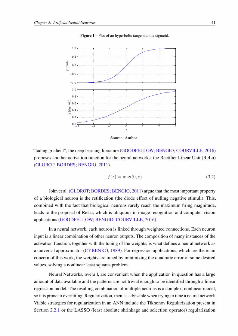
Chapter 3. Artificial Neural Networks 41
Figure 1 – Plot of an hyperbolic tangent and a sigmoid.
−1.0
−0.5
0.0
0.5
1.0
y (
tanh)
−3 −2 −1 0 1 2 3z
0.0
0.2
0.4
0.6
0.8
1.0
y (
sigm
oid
)
Source: Author.
“fading gradient”, the deep learning literature (GOODFELLOW; BENGIO; COURVILLE, 2016)
proposes another activation function for the neural networks: the Rectifier Linear Unit (ReLu)
(GLOROT; BORDES; BENGIO, 2011).
f(z) = max(0, z) (3.2)
John et al. (GLOROT; BORDES; BENGIO, 2011) argue that the most important property
of a biological neuron is the retification (the diode effect of nulling negative stimuli). This,
combined with the fact that biological neurons rarely reach the maximum firing magnitude,
leads to the proposal of ReLu, which is ubiquous in image recognition and computer vision
applications (GOODFELLOW; BENGIO; COURVILLE, 2016).
In a neural network, each neuron is linked through weighted connections. Each neuron
input is a linear combination of other neuron outputs. The composition of many instances of the
activation function, together with the tuning of the weights, is what defines a neural network as
a universal approximator (CYBENKO, 1989). For regression applications, which are the main
concern of this work, the weights are tuned by minimizing the quadratic error of some desired
values, solving a nonlinear least squares problem.
Neural Networks, overall, are convenient when the application in question has a large
amount of data available and the patterns are not trivial enough to be identified through a linear
regression model. The resulting combination of multiple neurons is a complex, nonlinear model,
so it is prone to overfitting. Regularization, then, is advisable when trying to tune a neural network.
Viable strategies for regularization in an ANN include the Tikhonov Regularization present in
Section 2.2.1 or the LASSO (least absolute shrinkage and selection operator) regularization

Chapter 3. Artificial Neural Networks 42
Figure 2 – Representation of a Feedforward Neural Network with 3 inputs, 2 hidden layers with 4 neurons each,and 2 outputs. Each arrow represents a weighted connection between each neuron, represented by acircle.
Input Layer Hidden Layers Output Layer
Source: Author.
(TIBSHIRANI, 1996). While Tikhonov utilizes ℓ2-norm, LASSO utilizes ℓ1-norm and is able to
obtain networks with sparse weights, significantly reducing model complexity.
3.2 FEEDFORWARD NEURAL NETWORKS
The most basic type of neural networks are the Feedforward Neural Networks (also
referred to as Multilayer Perceptron (MLP)). The main characteristic of these networks is that,
since the value of each neuron does not depend on itself in previous instants in time, they are
memoryless, or static. To ease gradient calculation and function evalutation, it is rather common
to see the neurons organized in layers.
Figure 2 depicts a generic feedforward neural network. A neural network is described by
the following equations:
y = f(Wnlznl
) (3.3)
znl = f(Wnl−1znl−1) (3.4)
zn = f(Wn−1zn−1) (3.5)
z1 = f(W0u) (3.6)
where zn corresponds to the vector where each element is a neuron of layer n. The network has
nl layers. u is the input and y is the output vector. The matrix W0 define the weights between the
input layer and the first hidden layer. The matrix Wn gives the weights between layer n and layer
n+ 1. The vector function f(·) is the element-wise activation function, which is considered to be

Chapter 3. Artificial Neural Networks 43
generic for this analysis, but functions such as tanh() or the sigmoid as presented in Equation
(3.1). Bias can be naturally added to this formulation by concatenating the input vector u and
each layer vector zn with 1 and adding a corresponding weight vector to it. A neural network
that has a large nl, that is, a large number of layers, is considered a Deep Neural Network.
In a neural network, the trainable weights are represented by the elements in each matrix
Wn where the index n = {0, 1, ..., nl}. For the purpose of optimization, consider a vector w
that is essentially every matrix Wn flattened. For regression, the task of interest in this work,
the objective is to minimize the quadratic error between the desired output y and the expected
output y(w,u) (for simplicity, assume there is only one output):
E(w,u) =1
2(y − y(w,u))2 (3.7)
Calculating the gradient in a neural network was an impeding task in the early years, up
until the error Backpropagation algorithm was invented (NELLES, 2001). Backpropagation is
essentially the use of the chain rule to calculate the gradient, facilitated by the layered structure
of the network. The derivative of the cost function with respect to w is:
∂E
∂w= (y − y(w,u))
∂y
∂w(3.8)
The value for ∂y
∂wdepends on which layer the weights are. If the weights are at the output
layer, then the answer is trivial (since y, Wnlis a row vector):
∂y
∂Wnl
= f ′(Wnlznl
)zTnl
(3.9)
For y with respect to an arbitrary hidden layer weight matrix Wn it is:
∂y
∂Wn
=∂y
∂an
znT (3.10)
with an = Wnzn. The calculation of ∂y
∂ancan be done recursively:
∂y
∂an
=∂an+1
∂an
T ∂y
∂an+1
= f ′(an)Wn+1T ∂y
∂an+1
(3.11)
It is known that ∂y
∂anl
= f ′(anl), so this information is used to calculate the gradient of
the previous layer, so on and so forth. To initialize the algorithm, it is advisable that the weights
are started randomly. Since the algorithms solve a nonlinear optimization problem, a random
initialization could lead the network to a better local minimum, as starting all the weights as 0
could bind the network to a bad local optimum (BISHOP, 2006).
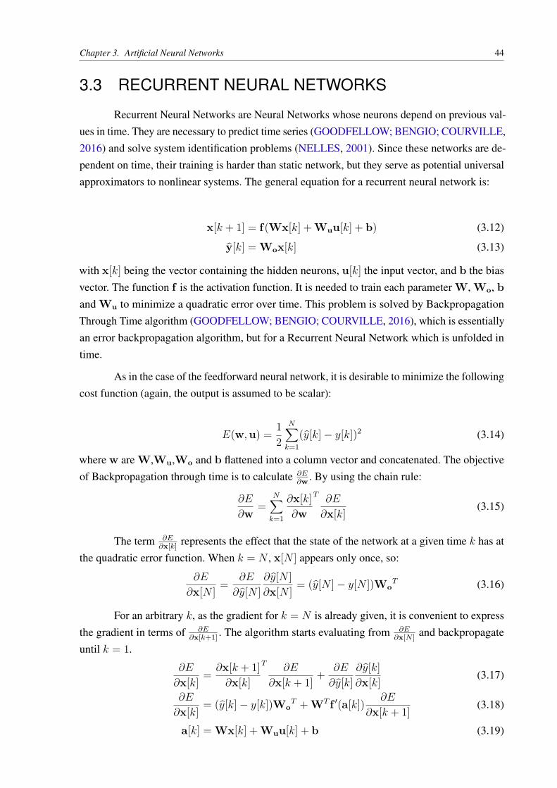
Chapter 3. Artificial Neural Networks 44
3.3 RECURRENT NEURAL NETWORKS
Recurrent Neural Networks are Neural Networks whose neurons depend on previous val-
ues in time. They are necessary to predict time series (GOODFELLOW; BENGIO; COURVILLE,
2016) and solve system identification problems (NELLES, 2001). Since these networks are de-
pendent on time, their training is harder than static network, but they serve as potential universal
approximators to nonlinear systems. The general equation for a recurrent neural network is:
x[k + 1] = f(Wx[k] + Wuu[k] + b) (3.12)
y[k] = Wox[k] (3.13)
with x[k] being the vector containing the hidden neurons, u[k] the input vector, and b the bias
vector. The function f is the activation function. It is needed to train each parameter W, Wo, b
and Wu to minimize a quadratic error over time. This problem is solved by Backpropagation
Through Time algorithm (GOODFELLOW; BENGIO; COURVILLE, 2016), which is essentially
an error backpropagation algorithm, but for a Recurrent Neural Network which is unfolded in
time.
As in the case of the feedforward neural network, it is desirable to minimize the following
cost function (again, the output is assumed to be scalar):
E(w,u) =1
2
N∑
k=1
(y[k] − y[k])2 (3.14)
where w are W,Wu,Wo and b flattened into a column vector and concatenated. The objective
of Backpropagation through time is to calculate ∂E∂w
. By using the chain rule:
∂E
∂w=
N∑
k=1
∂x[k]
∂w
T ∂E
∂x[k](3.15)
The term ∂E∂x[k]
represents the effect that the state of the network at a given time k has at
the quadratic error function. When k = N , x[N ] appears only once, so:
∂E
∂x[N ]=
∂E
∂y[N ]
∂y[N ]
∂x[N ]= (y[N ] − y[N ])Wo
T (3.16)
For an arbitrary k, as the gradient for k = N is already given, it is convenient to express
the gradient in terms of ∂E∂x[k+1]
. The algorithm starts evaluating from ∂E∂x[N ]
and backpropagate
until k = 1.
∂E
∂x[k]=∂x[k + 1]
∂x[k]
T ∂E
∂x[k + 1]+
∂E
∂y[k]
∂y[k]
∂x[k](3.17)
∂E
∂x[k]= (y[k] − y[k])Wo
T + WT f ′(a[k])∂E
∂x[k + 1](3.18)
a[k] = Wx[k] + Wuu[k] + b (3.19)
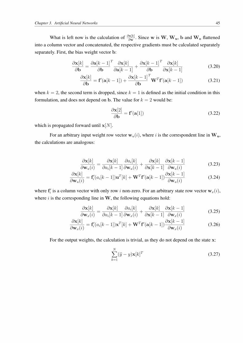
Chapter 3. Artificial Neural Networks 45
What is left now is the calculation of ∂x[k]∂w
. Since w is W, Wu, b and Wo flattened
into a column vector and concatenated, the respective gradients must be calculated separately
separately. First, the bias weight vector b:
∂x[k]
∂b=∂a[k − 1]
∂b
T ∂x[k]
∂a[k − 1]+∂x[k − 1]
∂b
T ∂x[k]
∂x[k − 1](3.20)
∂x[k]
∂b= f ′(a[k − 1]) +
∂x[k − 1]
∂b
T
WT f ′(a[k − 1]) (3.21)
when k = 2, the second term is dropped, since k = 1 is defined as the initial condition in this
formulation, and does not depend on b. The value for k = 2 would be:
∂x[2]
∂b= f ′(a[1]) (3.22)
which is propagated forward until x[N ].
For an arbitrary input weight row vector wu(i), where i is the correspondent line in Wu,
the calculations are analogous:
∂x[k]
∂wu(i)=
∂x[k]
∂ai[k − 1]
∂ai[k]
∂wu(i)+
∂x[k]
∂x[k − 1]
∂x[k − 1]
∂wu(i)(3.23)
∂x[k]
∂wu(i)= f ′
i(ai[k − 1])uT [k] + WT f ′(a[k − 1])∂x[k − 1]
∂wu(i)(3.24)
where f ′i is a column vector with only row i non-zero. For an arbitrary state row vector wx(i),
where i is the corresponding line in W, the following equations hold:
∂x[k]
∂wx(i)=
∂x[k]
∂ai[k − 1]
∂ai[k]
∂wx(i)+
∂x[k]
∂x[k − 1]
∂x[k − 1]
∂wx(i)(3.25)
∂x[k]
∂wx(i)= f ′
i(ai[k − 1])xT [k] + WT f ′(a[k − 1])∂x[k − 1]
∂wx(i)(3.26)
For the output weights, the calculation is trivial, as they do not depend on the state x:
N∑
k=1
(y − y)x[k]T (3.27)
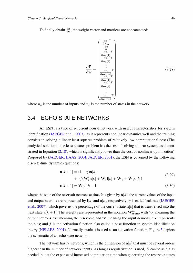
Chapter 3. Artificial Neural Networks 46
To finally obtain ∂E∂w
, the weight vector and matrices are concatenated:
∂E
∂w=
∂E∂Wo
T
∂E∂b
∂E∂wu(1)
T
∂E∂wu(2)
T
...∂E
∂wu(nu)
T
∂E∂wx(1)
T
∂E∂wx(2)
T
...∂E
∂wx(nx)
T
(3.28)
where nu is the number of inputs and nx is the number of states in the network.
3.4 ECHO STATE NETWORKS
An ESN is a type of recurrent neural network with useful characteristics for system
identification (JAEGER et al., 2007), as it represents nonlinear dynamics well and the training
consists in solving a linear least squares problem of relatively low computational cost (The
analytical solution to the least squares problem has the cost of solving a linear system, as demon-
strated in Equation (2.18), which is significantly lower than the cost of nonlinear optimization).
Proposed by (JAEGER; HAAS, 2004; JAEGER, 2001), the ESN is governed by the following
discrete-time dynamic equations:
a[k + 1] = (1 − γ)a[k]
+ γf(Wrra[k] + Wr
i i[k] + Wrb + Wr
oo[k])(3.29)
o[k + 1] = Wor a[k + 1] (3.30)
where: the state of the reservoir neurons at time k is given by a[k]; the current values of the input
and output neurons are represented by i[k] and o[k], respectively; γ is called leak rate (JAEGER
et al., 2007), which governs the percentage of the current state a[k] that is transferred into the
next state a[k + 1]. The weights are represented in the notation Wtofrom, with "o" meaning the
output neurons, "r" meaning the reservoir, and "i" meaning the input neurons. “b” represents
the bias; and f is the activation function also called a base function in system identification
theory (NELLES, 2001). Normally, tanh(·) is used as an activation function. Figure 3 depicts
the schematic of an echo state network.
The network has N neurons, which is the dimension of a[k] that must be several orders
higher than the number of network inputs. As long as regularization is used, N can be as big as
needed, but at the expense of increased computation time when generating the reservoir states

Chapter 3. Artificial Neural Networks 47
Figure 3 – Representation of an Echo State Network. Dashed connections (from Reservoir to Output Layer) aretrainable, while solid connections are fixed and randomly initialized.
.
.
.
.
.
.
i[k] o[k]
a[k]
Reservoir
Input Layer Output Layer
Source: Extracted from (JORDANOU et al., 2017), made by author.
according to Equation (3.29). According to (JAEGER, 2002), the ESN has a memory capacity
(MC) bounded by the number of neurons in the reservoir (MC ≤ N ), assuming that linear
output units are used.
The recurrent reservoir should have the so-called Echo State Property (ESP) (JAEGER,
2001), i.e., a fading memory of its previous inputs, meaning that influences from past inputs
on the reservoir states vanish with time. The ESP is guaranteed for reservoirs with tanh(·) as
the activation function when the singular values of Wrr < 1. However, this restriction limits the
richness of the reservoir dynamical qualities, and is not used in practice. Note that all connections
going to the reservoir are randomly initialized, usually according to the following steps:
1. Every weight of the network is initialized from a normal distribution N (0, 1).
2. Wrr is scaled so that its spectral radius ρ (Eigenvalue with the largest module) is at a certain
value which is able to create reservoirs with rich dynamical capabilities. It has been often
observed that setting ρ < 1 in practice generates reservoirs with the ESP (JAEGER et al.,
2007). However, reservoirs with ρ > 1 can still have the ESP since the effective spectral
radius may still be lower than 1 (OZTURK; XU; PRíNCIPE, 2007; VERSTRAETEN;
SCHRAUWEN, 2009).
3. Wri and Wr
b are multiplied by scaling factors f ri and f r
b , respectively, to determine how
the input will influence the network.
These scaling parameters, ρ and f ri , f r
b are crucial in the learning performance of the

Chapter 3. Artificial Neural Networks 48
network, having an impact on the nonlinear representation and memory capacity of the reservoir
(VERSTRAETEN et al., 2010). Also, low leak rates allow for higher memory capacity in
reservoirs, while high leak rates should be used for quickly varying inputs and/or outputs. The
settings of these parameters should be such that the generalization performance of the network
(loss on a validation set) is enhanced.
While in standard RNNs all weights are trained iteratively using backpropagation through
time (MOZER, 1995), ESNs restrict the training to the output layer Wor . In this work, reservoirs
have no feedback from the output, i.e., Wro = 0. Note that when the output feedback Wr
oo[k] is
present, the properties that guarantee ESP are different.. Also, the inputs do not interfere directly
in the output, as systems with direct transmission are less smooth and more sensitive to noise.
3.5 SUMMARY
This section presented Neural Networks and their Recurrent Counterparts. The static,
feedforward case was shown and backpropagation was introduced. The section also discussed
Recurrent Neural Networks and Backpropagation Through Time. In the end, a subtype of
Recurrent Neural Network was shown that does not need to use a complex algorithm such as
the Backpropagation Through Time: The Echo State Network. The ESN is ubiquous in this
work, as it is used as the inverse model to be learned in the Online Learning Controller and the
identification model for the Practical Nonlinear Model Predictive Controller.
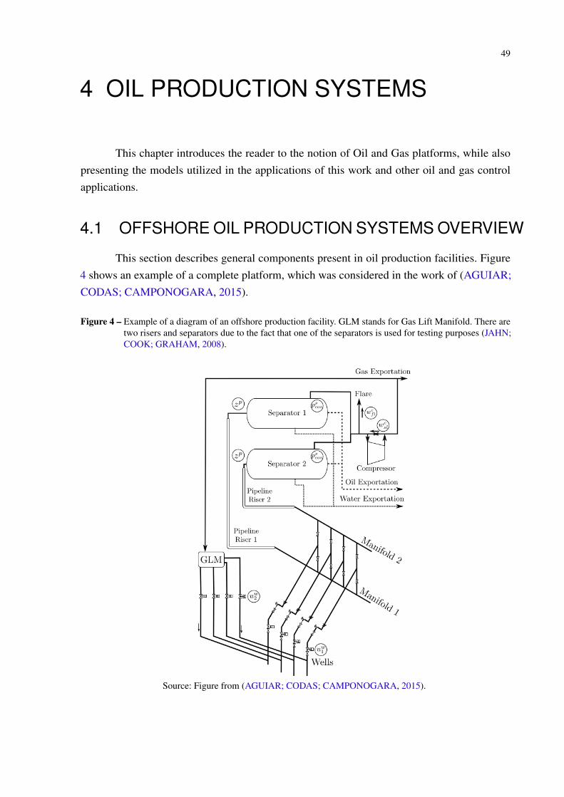
49
4 OIL PRODUCTION SYSTEMS
This chapter introduces the reader to the notion of Oil and Gas platforms, while also
presenting the models utilized in the applications of this work and other oil and gas control
applications.
4.1 OFFSHORE OIL PRODUCTION SYSTEMS OVERVIEW
This section describes general components present in oil production facilities. Figure
4 shows an example of a complete platform, which was considered in the work of (AGUIAR;
CODAS; CAMPONOGARA, 2015).
Figure 4 – Example of a diagram of an offshore production facility. GLM stands for Gas Lift Manifold. There aretwo risers and separators due to the fact that one of the separators is used for testing purposes (JAHN;COOK; GRAHAM, 2008).
Source: Figure from (AGUIAR; CODAS; CAMPONOGARA, 2015).

Chapter 4. Oil Production Systems 50
4.1.1 The Wells
A well is an apparatus responsible for conducting oil and gas from the reservoir to the
surface. Figure 5 shows the example of an offshore oil well. The tubulation in the well needs
to have the flow capacity for production (or injection) and be robust facing problems such as
sand production, corrosion, high pressures or temperatures, mechanical failure and production
chemistry issues such as waxes, scales and hydrates (JAHN; COOK; GRAHAM, 2008). A
production platform can have one or more wells. This number is obtained during tests on the
appraisal phase of the oil field. A well which is able to produce oil at a commercial rate without
help from a lifting system is called a natural flowing well (JAHANSHAHI, 2013).
This work considers a vertical, offshore well, operated using gas lift. Gas lift consists
in reinjecting produced gas into the well, thus lowering the density of the produced fluid and
easening its ascent, increasing the production flow (JAHN; COOK; GRAHAM, 2008; AGUIAR;
CODAS; CAMPONOGARA, 2015). A gas-lifted well can be split in two different parts: the
annulus, which is the medium where the gas for gas lift is injected, and the tubing, where flows
the produced fluid. The gas used for gas lift comes from a valve which controls the amount of
gas injected, passes through the annulus and goes to the tubing through an injection valve.
In each well, production tests are performed at least once per month by diverting the
production for certain measurements in the test separator. Measurements for testing include the
tubing head pressure, the flow, the velocity distribution, the consistency with the used simulation
model, and other factors.
4.1.2 Subsea Processing
Some wells are included with subsea processing. Wells tend to also produce water, which
is undesirable for commercial applications, so a separator is used to inject water back into the
ocean (JAHANSHAHI, 2013). Sand and other undesirable substances are also handled by the
subsea separator. This has shown improvements both in the production and in the top separation
efficiency (JAHANSHAHI, 2013).
4.1.3 Manifolds
If more than one well is used, it is expensive to directly send their production to the
surface, so they are connected directly to each other using a manifold. A manifold is the
component that connects the different wells associated with an oilfield, merging their flows into
one. This tubulation gathers all fluids which are being produced by the wells and direct the
mixture into a pipeline-riser system. This equipment must be properly designed to resist the
intensity of the flow coming from the most productive well.

Chapter 4. Oil Production Systems 51
Figure 5 – Schematic representation of the well considered in this work.
Gas lift
choke
Production
choke
Oil
outlet
Gas
inlet
Annulus
Injection
valve
Tubing
wG,in: Inlet gas mass flow rate
Pat: Annulus top pressure
Pab: Annulus bottom pressure
Pbh: Bottom-hole pressure
Ptt: Tubing top pressure
wout: Outlet mass flow rate
mix,t: Mixture density at top of tubing
L,t: Liquid volume fraction at top
u1: Opening of production choke
u2: Opening of gas lift choke
Pres: Reservoir pressurePgs : Gas lift source pressure
Pres
Pgs
Ptt mix,t L,t
Pat
Pbh
u1
u2wG,in
wout
Pab
ρ
α
ρ α
Source: Adapted from (JAHANSHAHI; SKOGESTAD; HANSEN, 2012).
4.1.4 Pipeline-Riser
This is the structure responsible for bringing the produced reservoir fluid into the surface.
This structure can be considered as the blood vessel of an offshore oil platform (JAHANSHAHI,
2013).
In this work, it consists of a horizontal pipeline that receives fluid from the manifold as
inflow, and the outlet flow goes to what is called the Riser. The Riser is a vertical tubulation used
to transport fluid from the pipeline into the surface. These components incur a major cost in the
implementation of an oil field, due to the need to be specifically designed to certain temperature
and depth configuration (JAHANSHAHI, 2013). Figure 6 shows an example of pipeline-riser
system.

Chapter 4. Oil Production Systems 52
Figure 6 – Representation of a pipeline-riser system. Pout represents the pressure in the separator.
Source: Obtained from (JAHANSHAHI; SKOGESTAD; GRØTLI, 2013a).
4.1.5 Separator and Top-side Processing
The flow of a riser can come in three (or more) different phases: oil, gas or water. The
separator receives the flow as inlet and has the purpose of separating the flow into oil, gas or
water. The outflow will then be sent to the other processes in the top-side processing, and then
transported for selling and/or refining, or being discarded in an (ideally) environmental friendly
way.
Separators are classified into two-phased, if they separate the flow into gas and liquid, or
three-phased, if they separate crude oil into gas, water and oil.
The other units in the top-side processing are defined by a process engineer, which must
find the minimum necessary steps to turn crude oil into refinable products. Other processes
can include, degassing, dehydration (for oil), dew point conditioning, contaminant removal,
compression (for gas), and de-oiling (for water to be disposed).
4.1.6 Flow Assurance Issues
Assuming a complete production platform, there are several factors which can affect
production, costing millions of dollars to the oil company. This subsection is based on the
information from (JAHANSHAHI, 2013). Below is a list of effects that can affect the quality of
the fow in production.
• Hydrates: Crystaline materials where water molecules are mixed with certain gases or
gas mixtures, forming where the temperature is low and there is elevated pressure. This
substance can block gas flowlines. What is generally used is applying MEG (Mono-
ethylene Glycol) at the blocked area.
• Wax: A natural constituent in any crude oil and most gas condensates that increases the
oil viscosity, increases wall roughness, lessens flow and compromise storage. The most
usual strategy for Wax removal is pigging (JAHANSHAHI, 2013). Pigs is an entity used
to clean oil platform pipes, being described at (JAHN; COOK; GRAHAM, 2008).
• Asphaltenes: The heaviest fractions of crude oil. They can precipitate during production
due to changes of pressure, temperature and fluid composition. The precipitated particles

Chapter 4. Oil Production Systems 53
are then deposited in the pipeline, causing production rate decline and other operational
problems. The industrial solution to this problem is avoiding the operation point at which
asphaltene is precipitated.
• Scales: Deposits of inorganic salts, reducing capacity of the flowline. To deal with scales,
chemicals named “scale inhibitors” and “scale dissolvers” are applied.
• Corrosion: In fields which produce large quantities of water, pipe corrosion can be a
possible issue. Carbon steel is considered an economic solution for this problem.
• Emulsions: Emulsions can compromise separation efficiency and the processing facilities,
which can cause loss in production. The solution to this is using de-emulsifiers.
• Slugging Flow: Happens due to gas and liquid being transported at the same time, more is
explained below.
4.1.7 Slugging Flow
Gas and liquid phases normally do not travel at same velocity in the pileline. This is due
to differences in density and viscosity. For an upward flow, such as in a riser, the gas phase flows
at a higher velocity than the liquid phase. Also, predicting how a multiphase composition will
flow is a complex task, even in a simple pipeline geometry.
Slug flow can be caused by either of these factors (JAHANSHAHI, 2013):
• Hydrodynamics,
• The upward flow within a riser,
• Irregular surface of seabeds,
• Induction by pigging,
• Gas compression in the annulus of a gas lifted well,
• Accumulation of gas at the bottom of a long well.
The slugging induced by the presence of a riser is one of the most important flow as-
surance challanges. In slugging, liquid accumulates in the entrance to the riser, blocking gas
entrance, leading to the compression of the gas in the pipeline. Each instance of this accumulation
is called a slug. This happens if gas and liquid velocities are sufficiently low. The slug continues
to grow as the hydrostatic head of the liquid in the riser is higher than the pressure drop over the
riser (JAHANSHAHI, 2013). When the pressure drop over the riser exceeds the hydrostatic head
due to slug accumulation, the liquid is pushed out of the riser and, when all liquid has left the
riser, liquid falls back into the bottom due to low velocity and starts to accumulate again.
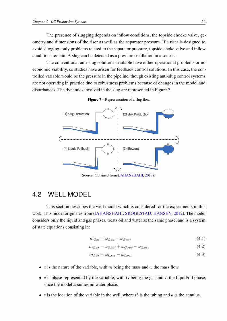
Chapter 4. Oil Production Systems 54
The presence of slugging depends on inflow conditions, the topside chocke valve, ge-
ometry and dimensions of the riser as well as the separator pressure. If a riser is designed to
avoid slugging, only problems related to the separator pressure, topside choke valve and inflow
conditions remain. A slug can be detected as a pressure oscillation in a sensor.
The conventional anti-slug solutions available have either operational problems or no
economic viability, so studies have arisen for feedback control solutions. In this case, the con-
trolled variable would be the pressure in the pipeline, though existing anti-slug control systems
are not operating in practice due to robustness problems because of changes in the model and
disturbances. The dynamics involved in the slug are represented in Figure 7.
Figure 7 – Representation of a slug flow.
(1) Slug Formation (2) Slug Production
(3) Blowout(4) Liquid Fallback
Source: Obtained from (JAHANSHAHI, 2013).
4.2 WELL MODEL
This section describes the well model which is considered for the experiments in this
work. This model originates from (JAHANSHAHI; SKOGESTAD; HANSEN, 2012). The model
considers only the liquid and gas phases, treats oil and water as the same phase, and is a system
of state equations consisting in:
mG,a = ωG,in − ωG,inj (4.1)
mG,tb = ωG,inj + ωG,res − ωG,out (4.2)
mL,tb = ωL,res − ωL,out (4.3)
• x is the nature of the variable, with m being the mass and ω the mass flow.
• y is phase represented by the variable, with G being the gas and L the liquid/oil phase,
since the model assumes no water phase.
• z is the location of the variable in the well, where tb is the tubing and a is the annulus.
Chapter 4. Oil Production Systems 55
If y is absent and the variable is in the form xz, then the variable does not describe a
specific phase. mG,a, mG,tb and mL,tb are the state variables considered in this model (in kg).
This model is also described in Figure 5. mG,a is the total mass of gas that is currently in the
annulus of the well. This is the gas that comes from the gas lift source, as represented by its state
equation: ωG,in is the mass flow (kg/s) of the gas coming from the source into the annulus. ωG,inj
is the mass flow (kg/s) of the annulus gas coming into the tubing. mG,tb is the total mass of gas
that is currently in the tubing of the well. It has two sources, ωG,inj and ωG,res, which is the gas
mass flow that comes from the reservoir. ωG,out is the outlet gas mass flow, which leaves the well
tubing into the platform or a manifold. mL,tb is the mass of liquid in the well tubing. The liquid
comes from the reservoir with mass inlet flow (kg/s) ωL,res and leaves with outlet mass flow
ωL,out.
These mass flows are computed using Bernouilli’s orifice equation:
ωGin = Kgsu2
√ρG,in max(Pgs − Pat, 0)
ωGinj = Kinj
√ρG,ab max(Pab − Ptb, 0)
ωout = Kpru1
√ρmix,t max(Ptt − P0, 0)
ωres = PI max(Pres − Pbh, 0)
ωL,res = (1 − αmG,b)ωres
ωG,res = αmG,bωres
ωL,out = (1 − αmG,t)ωout
ωG,out = αmG,tωout
These variables follow the notation according to Figure 5. Kgs,Kinj , and Kpr are experi-
mental variable parameters which depend on the practical application. P0 is the outlet pressure.
αmG,b is the mass fraction of the bottom flow, and αm
G,t is the mass fraction of the outlet flow. αmG,b
is assumed to be constant and u1 and u2, the choke valve opening and gas lift valve opening,
respectively, are the model inputs and manipulated variable candidates. αmG,t is calculated as:
αmG,t =
(1 − αL,t)ρG,t
αL,tρL + (1 − αL,tρG,t)
αL,t = 2αL − αL,b
αL,b =ωL,resρG,tb
ωL,resρG,tb + (ωG,inj + ωG, res)ρL
αL =mL,tb − ρLVbh
VtρL
where αL is the average liquid fraction inside the tubing, Vbh is the assumed volume at the
bottomhole, Vt is the volume in the tubing, and ρL, the liquid density, is assumed to be constant.
The other densities present in the previous equations are variable and calculated as follows,
derived from either the ideal gas law or the definition of density:

Chapter 4. Oil Production Systems 56
ρG,ab =PabMG
RTa
ρG,in =PgsMG
RTa
ρG,t =mG,tb
Vt + Vbh −mL,bh/ρL
ρmix =mG,tb +mL,tb − ρLVbh
Vt
ρG,tb =PtbMG
RTt
ρmix,t = αL,tρL + (1 − αL,t)ρG,t
with ρmix being the average mixture density inside the tubing, Ta and Tt the temperatures in
the annulus and tubing, assumed to be constant, R the universal gas constant, and MG the gas
molecular weight. The valve equations depend on the pressures, which are calculated as follows:
Pat =RTamG,a
MGVa
Pab = Pat +mg,agLa
Va
Ptt =ρG,tRTt
MG
Ptb = Ptt + ρmixgLt + Ft
Pbh = Ptb + Fb + ρLgLbh
The pressure Pat and Ptt are derived from the ideal gas law. Pab is Pat plus the gas’s
hydrostatic pressure. Pbh and Ptb contain not only the hydrostatic pressure imposed by the
liquid, but Fb and Ft, which are the pressure loss due to friction in the bottom-hole and the
tubing. La is the length of the annulus, Lt is the length of the tubing, and Lbh is the assumed
length of the bottom hole. Pres, Pgs and P0 are considered to be disturbances in this work.
These pressures depend on exogenous factors such as the reservoir, the gas lift source, and the
manifold, respectively, and can be potentially variable, but are considered to be initially constant
for modeling purposes. The pressure loss in the bottom-hole Fb is assumed to be constant, but
the pressure loss due to friction in the tubing Ft is calculated as:
Chapter 4. Oil Production Systems 57
Ft =λbρLU
2l,bLbh
2Dt
1√λt
= −1.8 log10
((ǫ
3.7Dt
)1.11
+6.9
Ret
)
Ret =ρmixUm,tDt
µ
Um,t = U sl,t + U sg,t
U sg,t =4(ωG,in + αm
G,bωres)
ρG,tπD2t
The above equations are derived from Haaland’s solution to the Colebrook-White equa-
tion (1983) for the calculation of the friction factor of the tubing λt. Ret is the Reynolds number
of the flow at the tubing. Um,t is the average velocity in the tubing, U sg,t is the average superficial
velocity of the gas phase. U sl,t is the average superficial velocity of the liquid phase, assumed to
be constant. Dt is the tube’s diameter, µ is the viscosity of the fluid. ωres is the assumed average
inlet flowrate, which is obtained experimentally and is constant for dynamics simplification
purposes.
The parameter values are set as follows for the simulation:
4.3 RISER
The pipeline-riser model utilized in this work was idealized in (JAHANSHAHI; SKO-
GESTAD, 2011). The same notation as the well model is used for the pipeline-riser model. This
model uses the same consideration as the well model: the model considers only a biphasic flow
consisting of liquid (oil and water) and gas phases. Since slugging is related to the velocity
difference between the gas and liquid phase, for anti-slug control applications, this model is rea-
sonable. The liquid phase is also assumed to be incompressible. This model approximates well to
an equivalent riser modeled in the OLGA commercial simulator (JAHANSHAHI; SKOGESTAD,
2011). The following state equations are considered:
mG,p = ωG,in − ωG,lp (4.4)
mL,P = ωL,in + ωL,lp (4.5)
mG,r = ωG,lp − ωG,out (4.6)
mL,r = ωL,lp + ωL,out (4.7)
(4.8)
The states represent:
• The total gas mass in the horizontal piping, mG,p.

Chapter 4. Oil Production Systems 58
Table 1 – Parameter values for the oil well
Parameter ValueMg: Molecular Gas Weight 0.0195 kg/molµ: Viscosity 3.64 × 10⁻³ Pa.sρL: Liquid Density 970 kg/m3
ǫ: Piping Superficial Roughness 2.8 × 10⁻⁵ mTa: Annulus Temperature 350 KVa: Annulus Volume 30.16 m3
La: Annulus Lenght 1500.0 mDa: Annulus Diameter 0.16 m2
Tt: Tubing Temperature 350 KVt: Tubing Volume 18.11 m3
Lt: Tubing Lenght 1500.0 mDt: Tubing Diameter 0.124 m2
U sl,t : Tubing Avarage Liquid Phase Velocity 0.163 m/sFb: Friction Loss in Bottom Hole 313 PaLbh: Length below Injection Point 75 mαm
G,b: Gas Mass Fraction at Bottomhole 4.58 × 10⁻²
ωres: Average Production Mass Flow 2.0 kg/sPr: Reservoir Pressure 250 × 105 PaPI: Reservoir Production Index 2.47 × 10⁻⁶ kg/(s.Pa)Kgs: Gas-Lift Choke Constant 1.6 × 10⁻⁴ kg/(s.Pa)Kinj: Injection Valve Constant 1.6 × 10⁻⁴ kg/(s.Pa)Kpr: Production Choke Constant 1.4 × 10⁻³ kg/(s.Pa)
Source: Obtained from (JAHANSHAHI; SKOGESTAD; HANSEN, 2012).
• The total liquid mass in the horizontal piping, mL,p.
• The total gas mass in the riser, mG,r.
• The total liquid mass in the riser, mL,r.
ωG,in is the inlet gas mass flow rate. ωG,lp is the gas mass flow rate of the fluid leaving the
pipeline and entering the riser. ωL,in is the inlet liquid mass flow rate. ωL,lp is the liquid mass
flow rate of the fluid leaving the pipeline and entering the riser. The acronym lp stands for “low
point”. ωG,out and ωL,out are the gas and liquid outlet mass flowrate, respectively, which then
goes to a top-side separator.
In the simulations featured in this work, ωG,in and ωL,in are boundary conditions assumed
to be constant, though these variables could be the outflow of a manifold connected to multiple
wells.
To calculate the outlet flow of the riser, the following equations are used:
Chapter 4. Oil Production Systems 59
ωout = Kpcz√ρt max(Pr − P0), 0
ωL,out = αmL,tωout
ωG,out = (1 − αmL,t)ωout
z is the production choke opening, which is the only possible manipulated variable in this model.
ωout is the total mass outlet flow. Pr is the pressure at the riser. αmL,t is the mass fraction at the
top of the riser. ρt is the density of the fluid at the top of the riser. P0 is the outlet pressure. Kpc
is a tuning parameter, regulated to approximate the dynamic of the model to a real life riser. The
top of the riser could be connected to a separator. To calculate αmL,t, ρt and Pr, these equations
are used:
αmL,t =
αL,t
ρt
ρt = αL,tρL + (1 − αL,t)ρG,r
Pr =ρG,rRTr
MG
where R is the universal gas constant, Tr is the assumed constant temperature in the riser. MG is
the gas molar weight. αL,t is the volume fraction of liquid at que top of the riser. ρG,r is the gas
density at the riser. ρL is the liquid density. To calculate αL,t and ρG,r these equations are used:
αL,t =2mL,r
VrρL
− AL
πr2p
ρG,r =mG,r
Vr −mL,r/ρL
Vr = πr2r(Lr + Lt)
Vr is the total volume of the riser; Lr represents the length of the riser; Lt is the length
between the top of the riser and the choke valve; AL is the area of liquid that is “blocking” gas
passage at the low-point; rp is the radius of the pipeline; rr is the radius of the riser; AL is
modeled as:
AL = πr2p − AG
AG =
πr2
p
(hp−hc
hc
)2hp < hc
0 hp ≥ hc
The area Ag represents the area free for gas passage in the low-point, hp represents the
height of liquid in the pipeline, and hc represents the critical height in which gas cannot pass

Chapter 4. Oil Production Systems 60
from the pipeline into the riser. As demonstrated by this equation, gas passage is not allowed in
the model when the height in the pipeline become higher than the critical height. hp is calculated
as follows:
hp = KhhcαL,p +
(ml,p − ρLVpαL,p
πr2p(1 − αL,p)ρL
)sin(θ)
αL,p =ρG,pωL,in
ρG,pωL,in + ρLωG,in
ρG,p =Pp,nomMG
RTp
Vp = πr2pLp
The variable αL,p is the average liquid volumetric fraction in the pipeline; Vp is the
volume of the pipeline; θ is the inclination angle of the pipeline in relation to the low-point; ρG,p
is the average gas density in the pipeline, assumed to be constant and calculated using Mg, which
is the gas molecular weight, R, the universal gas constant, Tp, the assumed constant temperature
of the pipeline, and Pp,nom, the assumed nominal pressure of the pipeline, obtained through
steady state experiments.
For calculation of the flows at the low-point, the following equations hold:
ωL,lp = KLAL
√ρL∆PL
ωG,lp = KGAG
√ρG,p∆PG
ρG,p =mg,p
Vp −mL,p/ρL
The parameters KG and KL are tunable gains to tune the model to behave as an experi-
mental application. ρG, p is the real gas density at the pipeline; ∆PL and ∆PG are the liquid and
gas pressure difference at the low point, respectively, and are calculated as follows:
∆PL = Pp − ∆Pfp + ρLghp − Pr − ρmgLr − ∆Pfr
∆PG = Pp − ∆Pfp − Pr − ρmgLr − ∆Pfr
Pp =ρG,pRTp
MG
ρm =mL,r +mG,r
Vr
in which Pp is the pressure at the pipeline; ρm is the average mixture density at the riser; g is
the gravity acceleration; ∆Pfr and ∆Pfp are the pressure loss due to friction for the riser and
pipeline respectively, and are calculated as:

Chapter 4. Oil Production Systems 61
∆Pfr =αL,rλrρmU
2m(Lr + Lt)
4rr
∆Pfp =αL,pλpρLU
2sl,inLp
4rp
αL,r =mL,r
VrρL
U sl,in =ωL,in
πr2pρL
Um =ωL,in
πr2rρL
+ωG,in
πr2rρG,r
The variable αL,r is the average liquid fraction at the riser. U sl,in is the average superficial
velocity of the inlet liquid. Um is the average superficial velocity of the mixture in the riser. λp
and λr are the friction factor of the pipeline and riser, respectively. They are calculated by the
following equation:
λx = 0.0056 + 0.5Re−0.32x (4.9)
in which x is either p, which stands for pipeline, or r, which stands for riser. Notably, the
calculation of the friction factor needs the Reynolds Number Re of the mixture in both the
pipeline or the riser. Re for each part of the system is calculated as follows:
Rep =2ρLU sl,inrp
µ
Rer =2ρmUmrr
µ
µ is the viscosity of the fluid, which is assumed to be constant. The model’s parameters
used are exactly the same as (JAHANSHAHI, 2013) and (JAHANSHAHI; SKOGESTAD, 2011),
due to it ensuring that the riser will endure severe slugging in these conditions. The inlet mass
flow is assumed to be 9 kg/s, in which 8.36 kg/s are from the liquid phase and 0.64 kg/s comes
from the gaseous phase. This implies gas accumulation in the low point due to the low velocity of
the gas phase. In these conditions, it is shown in (JAHANSHAHI; SKOGESTAD, 2011) that the
riser is only capable of attaining open loop production stability (detected by a constant pressure,
with the choke opening z ≤ 0.05). This low value for production is not adequate. According to
the biffurcation diagrams in (JAHANSHAHI; SKOGESTAD, 2011), this model’s limit cycle has
larger amplitude than the reference model from the commercial software OLGA used.
4.4 SYSTEM MODEL: TWO WELLS AND ONE RISER
The entity that connects the two wells and the riser is the Manifold. The manifold
considered in this work has no load loss due to friction, so the outlet pressure is equal to the two

Chapter 4. Oil Production Systems 62
gas-lift source gas-lift source
Well 2Well 1
Oil and Gas Reservoir
Manifold
Outlet
Riser
Riser Production Choke
gas-lift valve 1gas-lift valve2
Well Production Chokes
z
Figure 8 – Schematic of the complete oil and gas production system.
inlet pressures. This essentially means that the pressure at the outlet of both wells is equal to the
riser inlet pressure Pin, as defined in Eqn. (4.10):
Pin = Pw,out,1 = Pw,out,2 (4.10)
Given the conservation of mass, the sum of the outlet mass flow from the wells is equal
to the inlet flow of the riser.
ωG,in,r = ωG,out,w1 + ωG,out,w2 (4.11)
ωL,in,r = ωL,out,w1 + ωL,out,w2 (4.12)
where ωx,y,r is a mass flow in the riser and ωx,y,wi is a mass flow in well i.
The presence of the manifold then brings the complete system to possess: 10 state
variables, 110 algebraic variables, and 5 input variables. Due to the junction of the two wells
and the riser, the riser inlet flow and both well outlet pressures can no longer be considered
boundary conditions. In the end, the boundary conditions left for the complete system are: both
well gas-lift pressures Pgs,1 = 200 bar, and Pgs,2 = 200 bar, both well reservoir pressures Pr,1,
and Pr,2, and the riser outlet pressure, which is connected to the surface of a platform. As in
(JAHANSHAHI; SKOGESTAD, 2011), the outlet pressure is assumed to be 50.1 bar.
Figure 8 depicts a schematic representation of the complete plant, where the manifold
connects the two wells and the riser.
4.5 CONTROL APPLICATIONS IN OIL WELLS AND RIS-
ERS
In the literature, a lot of applications of control strategies involving production platform
plants can be found.

Chapter 4. Oil Production Systems 63
An example of a systemwide control, involving all the variables of the whole platform
in a simplified model, is (AGUIAR; CODAS; CAMPONOGARA, 2015). They sucessfuly use
optimal control theory applied in a whole oil production platform to maximize production
and reduce flare. The production maximization (using an economical objective function as
the performance function of the controller) and the smart tracking (a tracking cost function
penalizing the flare) manage to maintain optimal production with no need for flaring the gas. The
model of the platform used also assumes the scheduled maintenance of the compressor.
Another work, (PETIT, 2015), exposes examples of systems from the oil industry that
have variable delays and proposes an initial method on how to solve them.
In (CAMPOS et al., 2015), a real application of anti-slug control in both the Campos and
Santos basin is presented. The controller proposed in this paper is divided into three components:
• Diagnostic Module - For detection of severe slugs. Detected by oscillating pressures.
• Protection Module - For minimizing the damage done by slugs into external equipment. A
data-driven emergency choke-closing strategy.
• Anti-Slug Control - Module Responsible for minimizing or eliminating the slugs.
The work also proposes the use of some advanced control strategies such as the ONFC
(Online Neuro-Fuzzy COntroller), the gamma algorithm, and the commutational use of three
PIDs (Proportional - Integral - Differential) controllers.
In (OLIVEIRA; JÄSCHKE; SKOGESTAD, 2015), an adaptive control strategy is utilized
alongside supervisory control. The supervisory control consists in basically an oscillation detector
which increases the bottomhole pressure in presence of oscillations, and decreases the setpoint in
the abscence of oscillation, therefore driving the oil platform close to its limit. For the oscillation
detection, the algorithm checks if the frequency components of a fast Fourier transform (FFT)
have more energy at the neighborhood of the slug frequency. The adaptive control strategy
utilized is derived from the Model-Reference adaptive control, which is called Robust Adaptive
Control (OLIVEIRA; JÄSCHKE; SKOGESTAD, 2015). The controller assumes a state-space
linear model and uses a closed loop LQR controlled system as the reference model.
There is also the use of a control strategy which uses the derivative of the pipeline
pressure to supress the slug (PLUCENIO; CAMPOS; TEIXEIRA, 2015). The resulting strategy
is a simple, linear controller whose purpose is to bring the derivative of the bottom pressure
to zero. The aforementioned work also shows a mathematical proof on why a stable bottom
hole pressure is equivalent to no slug flow. They also estimate the variation in the bottom-hole
pressure based on a linear filter of the choke pressure, thus eliminating the need to measure the
pressure at the low-point.

Chapter 4. Oil Production Systems 64
Besides introducing the well model used in this work, (JAHANSHAHI; SKOGESTAD;
HANSEN, 2012) presents a robust control design for unstable regions in the well. The idea for
this controller is to find the linear parameters by solving an H∞ problem. Also, a controllability
analysis is made, which finds that the best performance of disturbance rejection in a SISO
(Single Input, Single Output) controller is when the bottomhole pressure is used as the controlled
variable and the well choke opening is used as the manipulated variable.
The work (JAHANSHAHI; SKOGESTAD; GRØTLI, 2013a) utilizes the same riser
model as (JAHANSHAHI; SKOGESTAD, 2011), but the parameters are changed so the limit
cycle happens when z = 0.15, in which z is the production choke opening at the top of the riser.
It focuses on the use of nonlinear observers for the task of estimating the states of the system
based on the riser top pressure, so that control could be applied directly to the system states,
testing techniques such as the Unscented Kalman Filter( UKF), which proved to be not robust
enough for the application. The use of a high-gain Luenberger observer is also tested, as an
alteration of the UKF which is called Fast Unscented Kalman Filter. The fast UFK is simply the
use of a coordinate transformation which Pr, the measured variable, is used as a state instead of
mgr. This is shown to increase robustness of the UKF. The control of the riser utilized in this
work managed to stabilize the pressure at an operation point at which z = 0.2. This was the
maximum production that could be achieved according to the paper.
Another work (JAHANSHAHI; SKOGESTAD; GRØTLI, 2013b) utilizes the same
model as (JAHANSHAHI; SKOGESTAD, 2011) with the same biffurcation diagram as (JA-
HANSHAHI; SKOGESTAD; GRØTLI, 2013a) (open-loop stability at z = 0.15). This paper
tries using output feedback linearization to stabilize the slugging flow in the riser, managing to
successfully stabilize the riser at z = 0.6, which is a good result.
For the control strategy of the well, this work uses the results from the controllability
analysis featured in (JAHANSHAHI; SKOGESTAD; HANSEN, 2012), which argues that the
best controllability happens when u1, the well outlet choke opening is used as the manipulated
variable, and pbh, the bottom-hole pressure, is used as the controlled variable. u2, the gas-lift
valve in which gas in injected into the annulus, is fixed at u2 = 0.4, as per (JAHANSHAHI;
SKOGESTAD; HANSEN, 2012). This also serves as a rough comparison to the performance
shown in (JAHANSHAHI; SKOGESTAD; HANSEN, 2012), though the parameters used for
this work are slightly different. The capacity of reference tracking and disturbance rejection in
this model using the control strategy depicted in Chapter 5 will be tested.
For the control strategy involving the pipeline-riser system, the controlled variable
used is the pp, which is the pressure at the pipeline, and the manipulated variable is z, the
production choke valve. The slug flow in the configuration of the model in (JAHANSHAHI;
SKOGESTAD, 2011) is more severe than in (JAHANSHAHI; SKOGESTAD; GRØTLI, 2013a)
and (JAHANSHAHI; SKOGESTAD; GRØTLI, 2013b), with maximum open-loop stability at
z = 0.05. The controller will test the lowest pressure in which the riser can be stabilized with,

Chapter 4. Oil Production Systems 65
in turn, testing the maximum choke opening z in which a maximum operating point can be
maintained.
4.6 SUMMARY
This chapter introduced the concept oil platforms and also the simulation models used
for application of both the Online Learning Controller and the ESN-based Model Predictive
Controller. Each component of an offshore oil platform is described, and were also exposed an
oil well and a riser model previously used in literature. For Chapter 5, the two wells - one riser
system is used as an application. For Chapter 6, only one gas-lifted oil well is utilized.

66
5 ON-LINE LEARNING CONTROL
This chapter introduces the online learning control. The online learning controller is a
black-box adaptive control strategy that uses Echo State Networks to identify an inverse model of
a plant, using no previous knowledge on physical information of the system. The inverse model
calculates the plant control action which is updated online through Recursive Least Squares.
The control methodology is applied in the two wells and one riser system described
in the previous chapter. First, this chapter describes the structure used in this control strategy.
Then, the challenges involving the application are shown, setting up different combinations
of manipulated variables and controlled variables. Lastly, this chapter presents the results of
applying the online-learning control into each application described, through diverse experiments.
5.1 DESCRIPTION
Originally proposed by Waegeman, Wyffels e Schrauwen (2012), the online-learning
controller is an adaptive control framework composed of two recurrent neural networks:
• ESN-L, the “ Learning Network ”, which learns parameters in an online way, and is
analogue to the “adaptive law” concept in an adaptive control framework (ASTROM;
WITTENMARK, 1994). The “ESN-L” takes both the present plant output (denoted as y[k]
in Figure 9) and a past plant output shifted δ timesteps to the past (denoted as y[k − δ]) as
the network input. Aiming at finding the inverse model, the output weights of the learning
network are trained at each timestep with such a data sample, by using the Recursive Least
Squares algorithm. The desired output of the network is fixed as u[k − δ], the control
action applied into the plant δ time steps before.
• ESN-C, the “ Control Network ”, computes the control action u[k], and is analogue
to the concept of the standard controller whose parameters are defined by the adaptive
law (ASTROM; WITTENMARK, 1994). The ESN-C output weights are copied from
ESN-L, and thus they correspond to the same inverse model (WAEGEMAN; WYFFELS;
SCHRAUWEN, 2012), which guarantees that, given that the plant current output is y[k],
the future output at time k+δ is y[k+δ] = y[k+δ], where y is the reference signal. Since
information learned from ESN-L is copied, ESN-C is essentially an approximation to the
inverse model which is used to compute u[k]. The input to ESN-C are the present plant
output y[k] and the desired plant output at δ time-steps into the future, which is referred
to as y[k + δ]. This is essentially the input to ESN-L, but displaced δ time-steps into the
future.

Chapter 5. On-line Learning Control 67
Figure 9 – Block diagram of the ESN-based control framework. Figure extracted from (JORDANOU et al., 2017).
ESN-C
ESN-L
S(x)
RLS
Plant
z-δ
a[k]Wro
Wro
u[k-δ]
Training
y[k]
u[k]ŷ[k+δ]
y[k-δ]
Source: Designed by the author. Used in (JORDANOU et al., 2017) and (JORDANOU; ANTONELO;CAMPONOGARA, 2019)
Figure 9 shows a block diagram representation of the control loop, which is composed of
the two aforementioned Echo State Network blocks. As shown in Figure 9, after being computed
by ESN-C, the unconstrained control action is processed by the constraint block S(x) block
before being input as u[k] to the plant and the Recursive Least Squares algorithm as illustrated in
Figure 9. This block represents the system constraints, such as saturation and rate limiting. The
timestep delay represented by δ is a tunable parameter of the framework, which is proportional to
the time constants of the system. A proof of convergence of this type of control loop is found in
(WAEGEMAN; WYFFELS; SCHRAUWEN, 2012). For inverse model training, the Recursive
Least Squares algorithm is used.
5.2 CONTROL CHALLENGES
The online-learning control was applied at the two wells - one riser system described in
Chapter 4, through the following control problems, which are all non-linear:
• Anti-Slugging Flow Control: The problem of controlling slugging flow consists mainly
in manipulating the riser choke in order to keep the riser inlet pressure constant (JAHAN-
SHAHI, 2013). The feedback control aims to avoid gas-liquid oscillations in the plant
outlet, which otherwise would bring about fluid flows that are difficult to process by the
FPSO (Floating Production Storage and Offloading) and even incur equipment damage in
extreme conditions. Preliminary simulations showed that an oscillatory regime can be in-
duced when the well gas-lift valves have choke openings with small differences. In Figure
10a, an open-loop test was carried out to qualitatively assess the dynamic properties of the

Chapter 5. On-line Learning Control 68
Figure 10 – Open loop test of the two wells, one riser system where the riser choke (blue line) is varied, and bothwell chokes (red and green line) are fully opened in a stable and an unstable case, dependent on thegas-lift choke openings
(a) Unstable case, where ugs,1 = 0.05 and ugs,2 = 0.00
88
90
92
94
96
98p_in (bar)
0 1000 2000 3000 4000 5000simulation time (min)
0.0
0.2
0.4
0.6
0.8
1.0
choke
s
(b) Stable case, where ugs,1 = 0.00 and ugs,2 = 0.00
90
95
100
p_in (bar)
0 200 400 600 800 1000 1200 1400simulation time (min)
0.0
0.2
0.4
0.6
0.8
1.0
choke
s
Source: Obtained by the author from simulations.
system at ugs,1 = 0.05 and ugs,2 = 0.0, where ugs,i stands for the gas-lift choke opening
of well number i. The results in this figure shows that the plant reaches stability only for a
riser choke opening z = 0.1, which is 10% of total production, or lower. In comparison,
the stable regime of ugs,1 = ugs,2 = 0, depicted in Figure 10b, was also tested. In this
case, although the system is stable, a control challenge arises from its highly nonlinear

Chapter 5. On-line Learning Control 69
behavior, as shown by the high variation of the static gain per operating point—the inlet
pressure increases exponentially as the choke opening becomes more constrained, as is
demonstrated in Figure 11. In the two conditions shown in Figure 10, only the riser choke
opening z is used to stabilize the riser inlet pressure Pin. The general objective of the
anti-slug control is to test the controller capacity to stabilize systems with oscillations.
• Super-Actuated Pressure Control: The gas-lift choke opening configuration is influential
on whether the plant will undergo pressure oscillations or not. In the previous control
problem, the plant was forced into a highly oscillatory regime to be suppressed by an
anti-slug controller, which manipulates only the riser choke opening. Instead in this task,
the anti-slug controller is allowed to manipulate the gas-lift choke openings (ugs,1 and
ugs,2) but not the production choke (z), which is fixed as fully open. This characterizes
a super-actuated control for having more manipulated variables than control variables.
Besides being easier to attain stability in the available setpoint range, due to the degrees of
freedom, the design of a black-box controller is challenging for having to avoid unstable
operating points, which might pose an issue since the model is previously unknown. In a
sense, this task serves as a test whether or not the controller can avoid unstable settings
and reach equilibrium for a wide variety of setpoints.
• Coupled Well Control: the objective is to control the two wells separately. Both wells
are coupled due to the presence of the manifold, which equates both well outlet pres-
sures. The well production choke valves are manipulated to control the bottom-hole
pressure of each well, but the gas-lift choke openings are held fixed at the value 0.4. In
real life, the measurement of the bottom-hole pressure is another problem by itself (JA-
HANSHAHI; SKOGESTAD; HANSEN, 2012) due to the low reliability of the involved
sensors. However, this can be mitigated by estimating the bottom-hole pressure (JAHAN-
SHAHI; SKOGESTAD; HANSEN, 2012), as done in (JAHANSHAHI; SKOGESTAD;
GRØTLI, 2013a) with a slugging riser. The challenge in this task emerges from the coupled
multivariate aspect of the problem, which was not explored in the previous tasks.
5.3 EXPERIMENTS AND RESULTS
This section showcases the experiments from the on-line learning controller of the oil
production plant (with two wells and one riser), which aims to test the controller capacity in
following setpoints and rejecting disturbances. Each of the control problems proposed in the
previous section was individually showcased.

Chapter 5. On-line Learning Control 70
Figure 11 – Static curve of the SISO-stable case, where the choke opening z is plotted against Pin in steady state.Each value of z brings the system to its correpondent value of Pin at the steady state.
0.0 0.2 0.4 0.6 0.8 1.0production choke opening (z)
88
90
92
94
96
98
100
102
steady state riser inlet pressure p_in
Static curve for the SISO case
Source: Obtained by the author from simulations.
5.3.1 Implementation
The plant model was implemented using Jmodelica, an open source dynamic system
modeling language which has an interface with Python 2.7. The Python libraries numpy and
scipy were used to implement both the Echo State Networks and the on-line learning controller.
The results were displayed using the matplotlib library. In all three cases, a sample time of 60
seconds was utilized.
5.3.2 Metrics and Experimental Setup
The metrics utilized in this work were defined in (HAFNER; RIEDMILLER, 2011), who
argue that a viable control metric is the average trajectory error eT of the controller:
eT =1
N
N∑
k=0
‖y[k] − y[k]‖1 (5.1)
where N is the total runtime in time steps, y[k] is the actual output and y is the predicted output.
Actually, this error metric is a term in the cost function for linear predictive control strategies
(CAMACHO; BORDONS, 1999), which uses the 2-norm instead of the 1-norm. Notice that the
average error eT is larger the longer the system takes to settle at a setpoint, being an indirect
evaluation of convergence time.
Because this metric fails to capture the transient behavior in the controller, such as
oscillations, it is proposed the use of the mean variation of the control action as an aditional
Chapter 5. On-line Learning Control 71
metric, which is also widely used in predictive control:
∆U =N∑
k=0
‖u[k] − u[k − 1]‖1 (5.2)
u[−1] = u0 (5.3)
In this metric, the variation ∆U increases if the control action differs between consecutive
timesteps, e.g. when system undergoes oscillations or during transients. In process control
applications, the behavior of the system must be as conservative as possible while respecting
process time constraints. So, the mean variation of the control action should be as low as possible.
In all experiments, the reference signal consists of three parts, each part having the
duration of 2000 time steps:
• the first part was designed to test the controller performance in different stable set points,
that vary gradually from one operating point to the next, and with no prior knowledge
of the model. This enables the controller to have more information about the different
operating points of the system and the step responses. Other setpoints could be used, such
as a sinusoidal setpoint or brown noise;
• the same setpoint signal was applied in the second part to test how the model evolves in
executing the same task, however now the controller uses the model that was learned in
the first part; and
• the third part applies a completely random signal, whereby both the amplitude and the
frequency of the signal vary. In the literature, this kind of signal is known as APRBS
(Amplitude modulated Pseudo-Random Binary Signal) (NELLES, 2001), where a PRBS is
modulated over a random amplitude, achieving, in the end, a random stair signal composed
of steps with random duration.
In control, better results are expected if the deviation from one setpoint to the next is
small, as advocated by the linear systems approximation theory (CHEN, 1998). So poor control
performance should be expected when the distance between one setpoint and the next is high.
The mean trajectory error eT and the total control variation ∆U are computed, for each
part of the simulation, which provides insights into how the controller has progressed. At each
time k, the metrics eT and ∆U are plotted over the 100 previous time steps, which shows how
the controller continuously progresses over time.
The metric eT is related to the IAE (Integral Absolute Error), which is a metric widely
applied in the literature (ASTROM; WITTENMARK, 1994; CAMACHO; BORDONS, 1999).
Chapter 5. On-line Learning Control 72
While the mean trajectory error eT describes a mean of absolute error, the IAE corresponds to a
summation. Therefore:
IAE =N∑
k=0
‖y[k] − y[k]‖1 = N × eT (5.4)
5.3.3 On Parameter Selection
Seven parameters of the ESN-based controller should be tuned: the prediction timestep
δ, the echo state network leak rate γ, the spectral radius ρ, the scaling of the network input and
bias weights, f ri and f r
b , respectively, the forgetting factor λ of the RLS algorithm, and α which
defines the initial RLS covariance matrix. The forgetting factor λ should be small enough so that
the RLS is sensitive to changes in the model, but large enough so that the covariance matrix P
does not degenerate. The value λ = (1 − 10−6) was chosen by trial and error. The behavior of
the main diagonal of the covariance matrix over time was analyzed and used as criteria to select
a value for λ sufficiently high to guarantee that P does not diverge, which otherwise causes
numerical instability, while maintaining the “forgetfulness” of past data by the RLS. A possible
hypothesis for the coveriance matrix diverging for values not as close to 1 as λ = (1 − 10−6)
is due to the large number of the inputs to the RLS (the number of ESN states, by the order of
hundreds). In normal filter applications for the RLS, a small forgetting factor (λ ≈ 0.94) would
be recommended for faster systems, but in this work, this was not shown to be the case.
When prior knowledge on the covariance matrix is unavailable, small values should be
selected for α in order to induce high covariance values, wich in turn express a high degree of
uncertainty. Notice also that a small value for α leads to a faster convergence rate of the RLS
algorithm. For the simulations herein α was set at 10−3. For each experiment the rest of the
parameters are described in Table 2. SISO corresponds to the experiments where the controlled
variable is the riser inlet pressure Pin and the manipulated variable is riser choke opening z,
for both the stable and the unstable case. MISO refers to the Pin control using both gas-lift
valves ugs,1 and ugs,2. MIMO refers to the control of both well downhole pressures Pbh,i by
manipulating the well production choke valves uch,i. For a fair comparison between parameters,
the reservoir is first initialized with random weights which are then fixed for parameter testing.
In all cases, 300 neurons proved to be enough to perform all the proposed tasks, consider-
ing learning and control of the system. A larger number of neurons requires more computational
power to calculate the control action, so it is desirable to keep the number of neurons sufficiently
low for the controller to learn the system.
A spectral radius ρ of of the reservoir weight matrix Wrr that is close to one, but not
outside the unit circle of the complex plane, is desirable to provide a large pool of dynamics
from the reservoir. The ESN state equation (3.29) is a linear system nested inside a nonlinear
piecewise activation function. If Wrr has eigenvalues larger the one, then the linear system inside
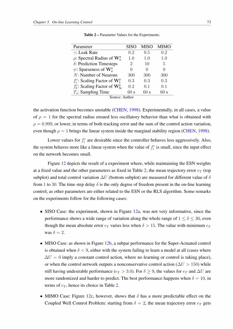
Chapter 5. On-line Learning Control 73
Table 2 – Parameter Values for the Experiments.
Parameter SISO MISO MIMOγ: Leak Rate 0.2 0.5 0.2ρ: Spectral Radius of Wr
r 1.0 1.0 1.0δ: Prediction Timesteps 2 10 5ψ: Sparseness of Wr
r 0 0 0N : Number of Neurons 300 300 300f r
i : Scaling Factor of Wri 0.3 0.3 0.3
f rb : Scaling Factor of Wr
b 0.2 0.1 0.1Ts: Sampling Time 60 s 60 s 60 s
Source: Author
the activation function becomes unstable (CHEN, 1998). Experimentally, in all cases, a value
of ρ = 1 for the spectral radius ensued less oscillatory behavior than what is obtained with
ρ = 0.999, or lower, in terms of both tracking error and the sum of the control action variation,
even though ρ = 1 brings the linear system inside the marginal stability region (CHEN, 1998).
Lower values for f ri are desirable since the controller behaves less aggressively. Also,
the system behaves more like a linear system when the value of f ri is small, since the input effect
on the network becomes small.
Figure 12 depicts the result of a experiment where, while maintaining the ESN weights
at a fixed value and the other parameters as fixed in Table 2, the mean trajectory error eT (top
subplot) and total control variation ∆U (bottom subplot) are measured for different value of δ
from 1 to 30. The time step delay δ is the only degree of freedom present in the on-line learning
control, as other parameters are either related to the ESN or the RLS algorithm. Some remarks
on the experiments follow for the following cases:
• SISO Case: the experiment, shown in Figure 12a, was not very informative, since the
performance shows a wide range of variation along the whole range of 1 ≤ δ ≤ 30, even
though the mean absolute error eT varies less when δ > 15. The value with minimum eT
was δ = 2.
• MISO Case: as shown in Figure 12b, a subpar performance for the Super-Actuated control
is obtained when δ < 9, either with the system failing to learn a model at all (cases where
∆U = 0 imply a constant control action, where no learning or control is taking place),
or when the control network outputs a nonconservative control action (∆U > 150) while
still having undesirable performance (eT > 3.0). For δ ≥ 9, the values for eT and ∆U are
more randomized and harder to predict. The best performance happens when δ = 10, in
terms of eT , hence its choice in Table 2.
• MIMO Case: Figure 12c, however, shows that δ has a more predictable effect on the
Coupled Well Control Problem: starting from δ = 2, the mean trajectory error eT gets

Chapter 5. On-line Learning Control 74
Figure 12 – Plot for eT (y axis of topmost plot) and ∆U (y axis of bottom plot) for different values of δ (x axis).
(a) δ variation experiment for the SISO case.
0
2
4
6
8
10
12
e_T
0 5 10 15 20 25 30delta
0
200
400
600
800
1000
1200
dU
(b) δ variation experiment for the MISO case.
0
5
10
15
20
25
e_T
0 5 10 15 20 25 30delta
0
50
100
150
200
dU
(c) δ variation experiment for the MIMO case.
0.0
0.5
1.0
1.5
2.0
2.5
3.0
3.5
4.0
e_T
0 5 10 15 20 25 30delta
0
20
40
60
80
100
120
140
dU
Source: Obtained by the author from simulations.
higher with δ. For 0 < δ < 10, the total control variation ∆U remains within an acceptable
range of [20, 40]. For the controllers where eT ≤ 0.5, δ = 5 induced the smallest ∆U .
The controller was not able to track the set points without the presence of bias (f rb = 0), invariably
incurring low performance. An analysis of bias values revealed that f rb = 0.2 produces better
results for the anti-slug cases, whereas a bias value f rb = 0.1 leads to good performed for the
super-actuated and coupled wells cases.
The SISO and MIMO applications were given a leak rate γ of 0.2, for having fast
dynamics, so there is no retardation of the controller dynamics related to the plant, and a spectral
radius ρ of 1.0, which ensure a long-lasting memory for the reservoir (slow dynamics are present).
The only parameters left to decide are ρ and γ for the MISO case, and δ for all three cases.
For the MISO case, the leak rate γ and spectral radius ρ were chosen by performing a
grid search for 0.3 ≤ ρ ≤ 1.2 and 0.1 ≤ γ ≤ 1 on discrete intervals of 0.1, considering both ∆U

Chapter 5. On-line Learning Control 75
Figure 13 – Color Grid for eT (a) and ∆U (b) for different values of γ (leak rate, y axis) and ρ (spectral ra-dius, x axis). Experiment done for the MISO case with the metrics evaluated during validation andgeneralization stages (last 4000 time steps).
(a) Mean Trajectory Error eT per grid element.
0.4 0.6 0.8 1.0 1.2spectral radius (rho)
0.1
0.2
0.3
0.4
0.5
0.6
0.7
0.8
0.9
1.0
leak rate (gamma)
e_T values
0.75
1.00
1.25
1.50
1.75
2.00
2.25
2.50
2.75
3.00
(b) Total Control Variation ∆U per grid element.
0.4 0.6 0.8 1.0 1.2spectral radius (rho)
0.1
0.2
0.3
0.4
0.5
0.6
0.7
0.8
0.9
1.0
leak rate (gamma)
dU values
0.00
20.00
40.00
60.00
80.00
100.00
120.00
140.00
160.00
180.00
200.00
Source: Obtained by the author from simulations.
and eT evaluated during the last 4, 000 time steps (validation and generalization phases) after the
initial training phase of 2, 000 time steps. Other parameters were fixed as shown in the Table 2.
The results of this batch of experiments are presented in Figure 13, where black corresponds to
high errors and white to low errors. For visualization purposes, we cut off points where eT > 3
and ∆U > 200 from the plot, where the performance was subpar, to better visualize the points
that performed good in terms of the two metrics. From the plot, we can notice that the optimal
combination of leak rate and spectral radius for the metric eT (where ∆U can be up to 100) is
located at γ = 0.5 and ρ = 1.0 (where eT < 0.6), while other parameter combinations have
led to more oscillatory behaviors in our analysis – represented by grey and black areas in the
total control variation plot in Figure 13b. Another view on the plot of ∆U is that, in general,
as ρ gets higher, the dynamics of the ESN is enriched with more nonlinearity and short-term
memory, causing the controller to behave more aggressively as well (darker areas of the plot).
However, the interplay between the spectral radius and the leak rate in this application is not
so evident, as the best blend of parameters takes place at γ = 0.5 and ρ = 1.0, suggesting a
nonlinear relationship between parameters for the best learning and control performance.
In addition, for γ < 0.5, the ESN state dynamics slows down too much for the controller
to effectively control the system – reflected by the top darker area with high error in Figure 13a.
We have also noticed that when γ > 0.7, the controller demonstrates behavior too aggressive to
properly stabilize the plant – verified by the darker area with high ∆U in Figure 13b. Although
the bottom left sections of the plots in Figure 13 (where 0.7 ≤ γ ≤ 0.6) have a greyish aspect
suggesting reasonable control performance, we have noticed that for these cases the covariance
matrix P has not decreased over time, i.e., the output weights learned by the RLS method have
high associated uncertainty (given by P) in the premature convergence of the RLS training.
As a result, the norm for Wor goes up over time, bringing about numerical instability for long
simulations.

Chapter 5. On-line Learning Control 76
There are other ways to tune the hyperparameters of a system, such as the Bayesian
Optimization (BROCHU; CORA; FREITAS, 2010).
5.3.4 Riser Inlet Pressure Stable SISO Control
The experiments herein concern the control of the riser inlet pressure Pin by manipulating
only the riser choke valve, arguably the simplest of the control problems for having only one
plant input and one plant output (SISO). The design of a linear controller for this problem is
particularly hard, since the static gain varies significantly from one operating point to another. Put
another way, a linear controller designed for an operating point can become unsuitable for another
point, however a static gain controller might solve that issue (ASTROM; WITTENMARK, 1994),
even though the dynamics are still nonlinear. No gas-lift is injected into the wells (ugs,1 = 0 and
ugs,2 = 0).
Before computing the control action, the network receives the feasible range of the inlet
pressure Pin scaled from [88.8, 95.0] bar to [−1, 1], for better numerical conditioning, whereby
88.8 bar is the riser inlet pressure for a fully open choke, and 95.0 bar is the pressure when the
choke is about 10% open. The control action is defined within the set [0.1, 1.0] to prevent the
well from being shut in. The control action set is then scaled to [−1, 1] to be in the same range as
the controlled variable.
The parameters for this case study are defined on the second column of Table 2, under
the heading SISO.
The third part of the simulation (from 4000 to 6000 time steps) was designed to have
low pressure setpoints, whereas high pressures were set for the first two parts of the simulation
(from 0 to 4000 time steps), as shown on the top plot of Figure 14. Within the third part of
the simulation, large changes in the riser choke opening imply small changes in the riser inlet
pressure. This behavior is shown in the top two plots of Figure 14. It can be noticed that the
controller can track the pressure profile within the third part, even though tracking was not
consistently kept at low pressures in the first two parts of the simulation. This happens due to
the fact that the models are being trained online, so the new data is being consistently fed to the
RLS.
Figure 14 shows the results of the stable SISO Pin control experiment. In the first subplot,
the red dashed line is the reference signal Pin and the blue solid line corresponds to the plant
output signal. After approximately 1000 time steps, the Echo State Network converged1 and was
able to thoroughly learn the system operating points. The ESN learning led the controller to
track the setpoints afterward with more damped dynamical behavior. This behavior is seen in the
first plot of Figure 14: the controller performs in the second part of the simulation the same task
of the first, however in a smoother manner, arguably because the RLS algorithm has processed1 The Echo State Network converges when the weights of the output layer stop changing drastically.
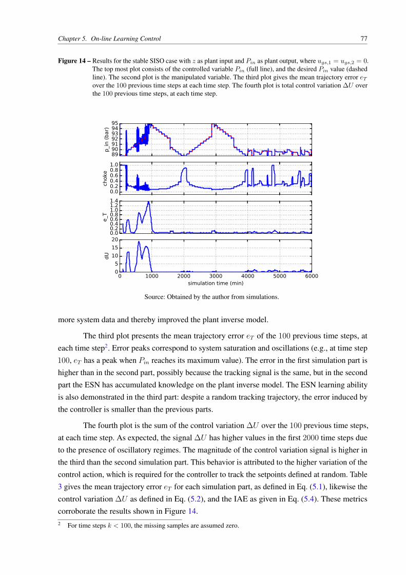
Chapter 5. On-line Learning Control 77
Figure 14 – Results for the stable SISO case with z as plant input and Pin as plant output, where ugs,1 = ugs,2 = 0.The top most plot consists of the controlled variable Pin (full line), and the desired Pin value (dashedline). The second plot is the manipulated variable. The third plot gives the mean trajectory error eT
over the 100 previous time steps at each time step. The fourth plot is total control variation ∆U overthe 100 previous time steps, at each time step.
89909192939495
p_in (bar)
0.00.20.40.60.81.0
choke
0.00.20.40.60.81.01.21.4
e_T
0 1000 2000 3000 4000 5000 6000simulation time (min)
0
5
10
15
20
dU
Source: Obtained by the author from simulations.
more system data and thereby improved the plant inverse model.
The third plot presents the mean trajectory error eT of the 100 previous time steps, at
each time step2. Error peaks correspond to system saturation and oscillations (e.g., at time step
100, eT has a peak when Pin reaches its maximum value). The error in the first simulation part is
higher than in the second part, possibly because the tracking signal is the same, but in the second
part the ESN has accumulated knowledge on the plant inverse model. The ESN learning ability
is also demonstrated in the third part: despite a random tracking trajectory, the error induced by
the controller is smaller than the previous parts.
The fourth plot is the sum of the control variation ∆U over the 100 previous time steps,
at each time step. As expected, the signal ∆U has higher values in the first 2000 time steps due
to the presence of oscillatory regimes. The magnitude of the control variation signal is higher in
the third than the second simulation part. This behavior is attributed to the higher variation of the
control action, which is required for the controller to track the setpoints defined at random. Table
3 gives the mean trajectory error eT for each simulation part, as defined in Eq. (5.1), likewise the
control variation ∆U as defined in Eq. (5.2), and the IAE as given in Eq. (5.4). These metrics
corroborate the results shown in Figure 14.2 For time steps k < 100, the missing samples are assumed zero.
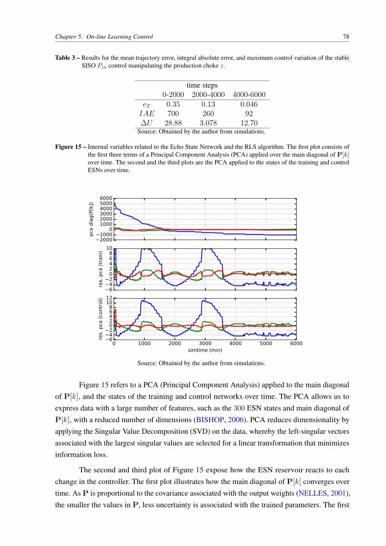
Chapter 5. On-line Learning Control 78
Table 3 – Results for the mean trajectory error, integral absolute error, and maximum control variation of the stableSISO Pin control manipulating the production choke z.
time steps0-2000 2000-4000 4000-6000
eT 0.35 0.13 0.046IAE 700 260 92∆U 28.88 3.078 12.70
Source: Obtained by the author from simulations.
Figure 15 – Internal variables related to the Echo State Network and the RLS algorithm. The first plot consists ofthe first three terms of a Principal Component Analysis (PCA) applied over the main diagonal of P[k]over time. The second and the third plots are the PCA applied to the states of the training and controlESNs over time.
−2000−1000
0100020003000400050006000
pca
dia
g(P
[k])
−6−4−2
02468
10
res.
pca
(tr
ain
)
0 1000 2000 3000 4000 5000 6000simtime (min)
−6−4−2
02468
1012
res.
pca
(co
ntr
ol)
Source: Obtained by the author from simulations.
Figure 15 refers to a PCA (Principal Component Analysis) applied to the main diagonal
of P[k], and the states of the training and control networks over time. The PCA allows us to
express data with a large number of features, such as the 300 ESN states and main diagonal of
P[k], with a reduced number of dimensions (BISHOP, 2006). PCA reduces dimensionality by
applying the Singular Value Decomposition (SVD) on the data, whereby the left-singular vectors
associated with the largest singular values are selected for a linear transformation that minimizes
information loss.
The second and third plot of Figure 15 expose how the ESN reservoir reacts to each
change in the controller. The first plot illustrates how the main diagonal of P[k] converges over
time. As P is proportional to the covariance associated with the output weights (NELLES, 2001),
the smaller the values in P, less uncertainty is associated with the trained parameters. The first
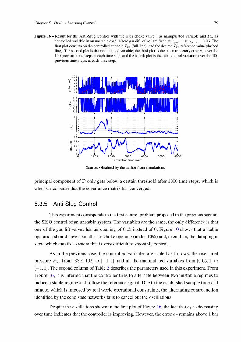
Chapter 5. On-line Learning Control 79
Figure 16 – Result for the Anti-Slug Control with the riser choke valve z as manipulated variable and Pin ascontrolled variable in an unstable case, where gas-lift valves are fixed at ugs,1 = 0; ugs,2 = 0.05. Thefirst plot consists on the controlled variable Pin (full line), and the desired Pin reference value (dashedline). The second plot is the manipulated variable, the third plot is the mean trajectory error eT over the100 previous time steps at each time step, and the fourth plot is the total control variation over the 100previous time steps, at each time step.
9092949698
100
p_in (bar)
0.00.20.40.60.81.0
choke
123456789
10
e_T
0 1000 2000 3000 4000 5000 6000simulation time (min)
0
5
10
15
20
\DeltaU
Source: Obtained by the author from simulations.
principal component of P only gets below a certain threshold after 1000 time steps, which is
when we consider that the covariance matrix has converged.
5.3.5 Anti-Slug Control
This experiment corresponds to the first control problem proposed in the previous section:
the SISO control of an unstable system. The variables are the same, the only difference is that
one of the gas-lift valves has an opening of 0.05 instead of 0. Figure 10 shows that a stable
operation should have a small riser choke opening (under 10%) and, even then, the damping is
slow, which entails a system that is very difficult to smoothly control.
As in the previous case, the controlled variables are scaled as follows: the riser inlet
pressure Pin, from [88.8, 102] to [−1, 1], and all the manipulated variables from [0.05, 1] to
[−1, 1]. The second column of Table 2 describes the parameters used in this experiment. From
Figure 16, it is inferred that the controller tries to alternate between two unstable regimes to
induce a stable regime and follow the reference signal. Due to the established sample time of 1
minute, which is imposed by real world operational constraints, the alternating control action
identified by the echo state networks fails to cancel out the oscillations.
Despite the oscillations shown in the first plot of Figure 16, the fact that eT is decreasing
over time indicates that the controller is improving. However, the error eT remains above 1 bar

Chapter 5. On-line Learning Control 80
which is considered high for the application. Table 4 reports the mean trajectory error, total
Table 4 – Results for the mean trajectory error, integral absolute error, and maximum control variation of theunstable SISO Pin control manipulating the production choke z.
time steps0-2000 2000-4000 4000-6000
eT 3.63 1.85 1.91IAE 7260 3700 3820∆U 158.53 158.76 177.22
Source: Obtained by the author from simulations.
control variation, and the integral absolute error for the three simulation parts.
By limiting the controller to manipulate only the riser choke valve, the controller failed
to stabilize the plant and track the reference signals. To fully overcome the oscillations, as other
stable configurations such as ugs,1 = ugs,2 = 0 exist, the controller needs to manipulate other
variables, which then would bring about more degrees of freedom. These super-actuated strategies
are more complex to learn, since many unstable operating points arise with the manipulation of
the gas-lift choke openings.
5.3.6 Super-Actuated Control
This section considers a controller with two manipulated variables, namely the gas-lift
chokes (ugs,1, ugs,2) while holding the riser choke fully open (z = 1) to sustain full oil production.
The goal is to track a reference signal for the riser inlet pressure Pin, being a control problem in
the MISO class.
Multiple solutions for reaching a given setpoint emerge from the additional degrees of
freedom, posing a challenge to learn the ESN-based inverse model. For example, a pressure of
120 bar can be achieved with multiple combinations of (ugs,1, ugs,2). As the input-output relation
is not bijective, the inverse model is not invertible and the controller must find an approximation
that works. Another challenge to control design stems from the slow system dynamics, since
a change on the gas-lift choke opening can take considerable time to influence the riser inlet
pressure.
The range for the riser pipeline pressure [100, 120] bar was scaled to [−1, 1], in which
100 bar is the lowest allowed pressure and 120 bar is the upper limit. The gas-lift choke opening
[0, 1] was likewise scaled to [−1, 1] for both valves.
The third column of Table 2 presents the parameters for this experiment. Figure 17
depicts the results of this experiment. Notice that the controller asymptotically stabilizes the
plant for nearly all setpoint once the RLS algorithm converges (showcased by the decrease of
eT , approximately after 1000 time steps, achieving better performance in the second simulation
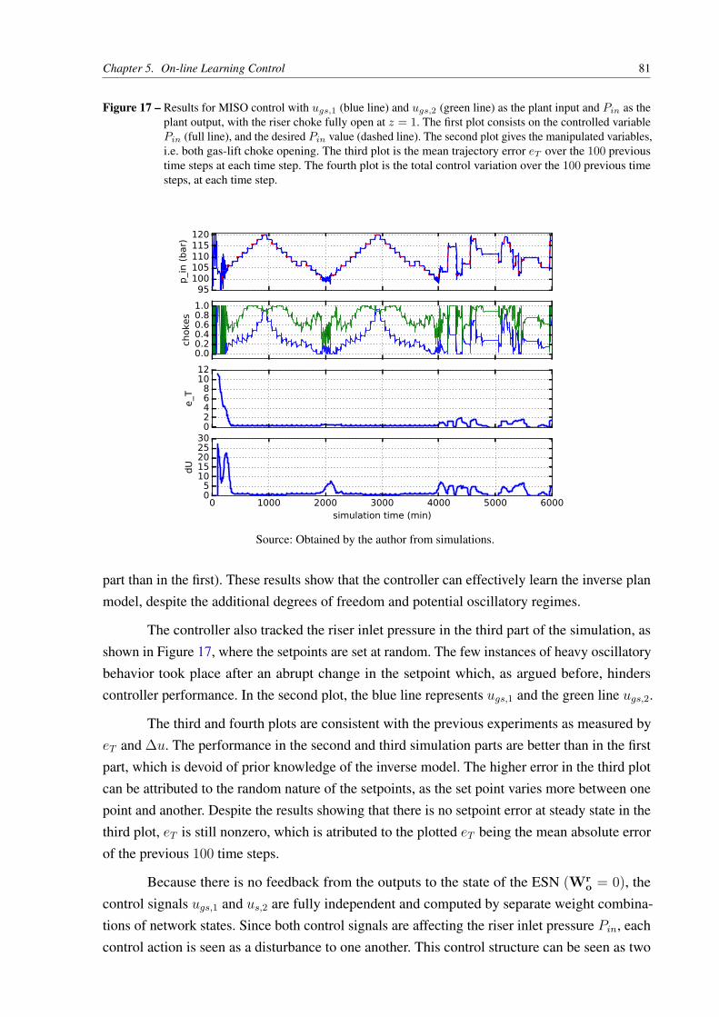
Chapter 5. On-line Learning Control 81
Figure 17 – Results for MISO control with ugs,1 (blue line) and ugs,2 (green line) as the plant input and Pin as theplant output, with the riser choke fully open at z = 1. The first plot consists on the controlled variablePin (full line), and the desired Pin value (dashed line). The second plot gives the manipulated variables,i.e. both gas-lift choke opening. The third plot is the mean trajectory error eT over the 100 previoustime steps at each time step. The fourth plot is the total control variation over the 100 previous timesteps, at each time step.
95100105110115120
p_in (bar)
0.00.20.40.60.81.0
chokes
02468
1012
e_T
0 1000 2000 3000 4000 5000 6000simulation time (min)
05
1015202530
dU
Source: Obtained by the author from simulations.
part than in the first). These results show that the controller can effectively learn the inverse plan
model, despite the additional degrees of freedom and potential oscillatory regimes.
The controller also tracked the riser inlet pressure in the third part of the simulation, as
shown in Figure 17, where the setpoints are set at random. The few instances of heavy oscillatory
behavior took place after an abrupt change in the setpoint which, as argued before, hinders
controller performance. In the second plot, the blue line represents ugs,1 and the green line ugs,2.
The third and fourth plots are consistent with the previous experiments as measured by
eT and ∆u. The performance in the second and third simulation parts are better than in the first
part, which is devoid of prior knowledge of the inverse model. The higher error in the third plot
can be attributed to the random nature of the setpoints, as the set point varies more between one
point and another. Despite the results showing that there is no setpoint error at steady state in the
third plot, eT is still nonzero, which is atributed to the plotted eT being the mean absolute error
of the previous 100 time steps.
Because there is no feedback from the outputs to the state of the ESN (Wro = 0), the
control signals ugs,1 and us,2 are fully independent and computed by separate weight combina-
tions of network states. Since both control signals are affecting the riser inlet pressure Pin, each
control action is seen as a disturbance to one another. This control structure can be seen as two

Chapter 5. On-line Learning Control 82
separate controllers manipulating the same variable and rejecting disturbances in the form of
multivariate coupling. Table 5 presents the metrics eT , ∆U , and IAE for each of the three parts
Table 5 – Results for the mean trajectory error, integral absolute error and maximum control variation of the Pin
control, manipulating the well gas-lift valves ugs,1 and ugs,2
time steps0-2000 2000-4000 4000-6000
eT 1.57 0.33 1.06IAE 3140 660 2120∆U 101.2 34.89 119.99
Source: Obtained by the author from simulations.
of the simulation. These metrics endorse the conclusion that were drawn above. For instance,
the control variation is higher in the third simulation part, which is a result of the control action
required to track a random changing set point.
5.3.7 Coupled Well Control
This experiment is the control of a MIMO plant consisting of both wells bottom-hole pres-
sure Pbh,i as controlled variables and each well production choke uch,i as manipulated variables,
which makes it the most complex experiment in terms of learning. Due to the multivariate nature
of the problem, some desired set-point combination might not be feasible, as the physics in the
plant impose operational constraints. The controller must find a feasible control action for each
pair of desired value related to the Pbh,i of each well. However, each input-output steady-state
gain varies less than in the riser per operating point, and the dynamics are well-behaved.
In this experiment, each well bottom-hole pressure is scaled from [170, 220], which are
the minimum and maximum bottom-hole pressure each well can reach, to [−1, 1]. Each well
production choke opening is scaled from [0.1, 1] to [−1, 1], with 0.1 being the lowest allowable
value for the well production chokes opening.
The fourth column of Table 2 shows the parameters utilized in this experiment. Figure
18 depicts the set-point tracking experiment. It took 500 time steps for the RLS to converge and
the inverse model to be learned. After the learning has converged, the controller tracked all the
proposed set-points with few oscillations in the control action, without prior knowledge, and even
considering coupling. Table 6 shows the total control variation and mean trajectory error over
the three phases of the simulation. These metrics corroborate the results previously discussed. In
Figure 19, the simulation applies a disturbance in the gas-lift source pressure of well 2 (Pgs,2),
which is shown on the bottommost plot. A step disturbance is an abrupt parametric change
in the model, occurring on a certain instant in time. The values for the disturbed variable are:
Pgs,2 = 200 bar until k = 3600, Pgs,2 = 170 bar until k = 3900, Pgs,2 = 230 bar until k = 4300,
and Pgs,2 = 200 for the rest of the simulation. A 30 bar disturbance is usually considered large for
linear control application. Even though the RLS algorithm converged, which leads the learning

Chapter 5. On-line Learning Control 83
Figure 18 – Result for MIMO control with uch,1 (blue line) and uch2 (green line) as input and Pbh,1 (blue line)and Pbh,2 (green line) as output. The first plot consists on the controlled variable Pbh (full line), andthe desired Pbh value for both wells (dashed line). The second plot is the manipulated variables, bothgas-lift choke opening, the third plot is the mean trajectory error eT over the 100 previous time steps ateach time step, and the fourth plot is total control variation over the 100 previous time steps, at eachtime step.
170180190200210220
p_b
h (bar)
0.00.20.40.60.81.0
choke
s
0
5
10
15
20
e_T
0 1000 2000 3000 4000 5000 6000simulation time (min)
05
10152025
dU
Source: Obtained by the author from simulations.
Table 6 – Results for the mean trajectory error, integrated absolute error and maximum control variation of theMIMO coupled wells control, without disturbances.
time steps0-2000 2000-4000 4000-6000
eT 2.96 0.421 1.62IAE 5920 842 3240∆U 28.2 3.84 27.9
Source: Obtained by the author from simulations.
algorithm to be less sensitive to changes in the plant, the controller still managed to compensate
for the parametric change in the model. This means that the on-line learning controller adapts
to model change with little to no hindrance in performance. Table 7 shows the result of this
Table 7 – Results for the mean trajectory error, integral absolute error and maximum control variation of the MIMOcoupled wells control, with disturbances.
time steps0-2000 2000-4000 4000-6000
eT 2.96 0.52 1.65IAE 5920 1040 3300∆U 28.2 7.11 23.8
Source: Obtained by the author from simulations.
experiment with disturbance applied. The disturbance is applied at the end of the second phase

Chapter 5. On-line Learning Control 84
Figure 19 – Result for MIMO control where a disturbance in Pgs,2 is applied, with uch,1 and uch2 as input and Pbh,1
and Pbh,2 as output, where z = 1 and ugs,1 = ugs,2 = 0.4. The first plot consists on the controlledvariable Pin (full line), and the desired Pbh value for both wells (dashed line). The second plot is themanipulated variables, both gas-lift choke opening, the third plot is the mean trajectory error eT overthe 100 previous time steps at each time step, and the fourth plot is total control variation over the100 previous time steps, at each time step. The fifth plot represents the step disturbance in the gas-liftsource pressure Pgs,2.
170180190200210220
p_b
h (bar)
0.00.20.40.60.81.0
choke
s
05
101520
e_T
05
10152025
dU
0 1000 2000 3000 4000 5000 6000simulation time (min)
170180190200210220230
p_g
s,2 (bar)
Source: Obtained by the author from simulations.
and beginning of the third phase. The fact that, in terms of error, the result did not change much,
means that the change of controlled system did not affect the performance very much. The higher
error in the second plot was due to poor reaction to the abrupt system change, which led to high
frequency oscillation.
5.4 SUMMARY
The on-line learning control framework from (WAEGEMAN; WYFFELS; SCHRAUWEN,
2012), based on Echo State Networks as substrate for learning an inverse model of a nonlinear
plant, is able to control complex simulated dynamical systems in a diverse set of scenarios
with no physical modeling information. The ESN-based controller was used to control an oil
production platform consisting of one riser and two wells connected by a manifold, where
complex dynamics were present such as steady-state gain variation, multiple degrees of freedom,
and coupled multi-variable control. Three control problems (SISO, MISO, and MIMO) involving
different plant variables were tackled, extending substantially previous work. The ESN-based
controller learned each different input-output dynamical behavior and performed set-point track-
ing and disturbance rejection, either explicitly or implicitly in multivariate coupling. Despite
the remarkable challenge of controlling a plant without a model, the online learning framework
has succeeded in all three proposes cases. Furthermore, the application of the learning controller

Chapter 5. On-line Learning Control 85
using a single flat ESN architecture has proved effective also for multivariate problems as shown
here, even when coupled variables were involved. For future works, stopping the updates of the
RLS mid simulation is also possible.

86
6 PRACTICAL NONLINEAR MODEL
PREDICTIVE CONTROL WITH
ECHO STATE NETWORKS
This chapter describes the control topology developed in (JORDANOU et al., 2018),
consisting in the practical nonlinear model predictive control (PLUCÊNIO et al., 2007) utilized
together with an Echo State Network as the predictive model. Echo State Networks have well
defined derivatives with respect to input signals, thus avoiding the on-line computation of the
finite difference algorithm to obtain the gradient, which was proposed in (PLUCÊNIO et al.,
2007). The advantage of the practical nonlinear model predictive control in relation to other
nonlinear approaches is that, even though the predictive model is nonlinear, the control action is
still computed by solving a Quadratic Programming (QP) problem, with satisfactory performance
(PLUCÊNIO et al., 2007). The approach can also be applied to any type of plant, without any
prior information, as long as the Echo State Network is able to provide a suitable model of it.
This control strategy was first tested in a gas-lifted oil well (JORDANOU et al., 2018).
6.1 PRACTICAL NONLINEAR MODEL PREDICTIVE CON-
TROL
Developed by Plucênio et al. (2007), the Practical Nonlinear Model Predictive Controller
(PNMPC) is a method that, through a first order Taylor expansion, separates a nonlinear generic
model into a free response and a forced response. The PNMPC has a computational advantage
over a generic Nonlinear MPC because the resulting control problem to be solved per iteration is
guaranteed to be a QP, similar to a linear MPC, whereas in the full nonlinear case a NLP would
be solved. This approach is advantageous when time constraints are in place. The PNMPC is
more or less akin to performing a one-step SQP in a quadratic cost function problem using a
nonlinear model. Assuming a dynamic system in the form:
x[k + i] = f(x[k + i− 1],u[k + i− 1]) (6.1)
y[k + i] = g(x[k + i]) (6.2)
u[k + i− 1] = u[k − 1] +i−1∑
j=0
∆u[k + j] (6.3)

Chapter 6. Echo State Networks for PNMPC 87
The prediction vectors in the PNMPC are:
Y = G · ∆U + F
∆U =
∆u[k]
∆u[k + 1]...
∆u[k +Nu − 1]
F =
g(f(x[k],u[k − 1]))
g(f(x[k + 1],u[k − 1]))...
g(f(x[k +Ny − 1],u[k − 1]))
G =
∂y[k+1]∂u[k]
0 . . . 0∂y[k+2]
∂u[k]∂y[k+2]∂u[k+1]
. . . 0...
.... . .
...∂y[k+Ny ]
∂u[k]∂y[k+Ny ]∂u[k+1]
. . . ∂y[k+Ny ]∂u[k+Nu−1]
where Ny is the prediction horizon and Nu is the control horizon. The derivatives inside G are
taken with respect to ∆u[k + i] = 0,∀i < Nu, and u represents the manipulated variable vector.
The vector ∆U consists in a concatenation of each control increment applied for calculation
of the prediction up until k = Nu. This structure is a vectorized form of the prediction along
the horizon, and is similar to the one depicted in Section 2.3.2 for the DMC and GPC, where
a similar vectorization of the prediction is made. The vector Y contains all the predictions
calculated by the model from k = 0 to k = Ny. As a consequence, the vector F contains all the
free responses calculated along the horizon, and the term G · ∆U is the forced response over
the prediction horizon. One possible alternative to the presented formulation is to concatenate
different prediction vectors for each input or output, which has the advantage of being able to
easily atribute a prediction and/or a control horizon to each variable, though in this work the
current formulation is preferred because it is more compact.
The equations above derive from the first-order Taylor series expansion in relation to
the manipulated variables, whereby the free-response F retains the nonlinearity, but the forced-
response is linearized so that the control increment is calculated through a quadratic program.
The matrix G is a result of that linearization, as each line corresponds to the first order term of
the Taylor approximation with respect to the control increment at a certain instant in time.
As Plucênio et al. (2007) assume a generic nonlinear system, they use a finite-difference
method to estimate the derivatives, which inherently suffers from combinatorial explosion when
multiple variables are involved. Having instead a system model whose derivatives are calculated
analytically, drastically reduces the computation time by mitigating this distavantage of finite
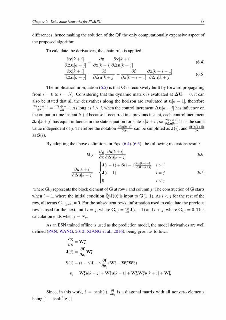
Chapter 6. Echo State Networks for PNMPC 88
differences, hence making the solution of the QP the only computationally expensive aspect of
the proposed algorithm.
To calculate the derivatives, the chain rule is applied:
∂y[k + i]
∂∆u[k + j]=
∂g
∂x[k + i]
∂x[k + i]
∂∆u[k + j](6.4)
∂x[k + i]
∂∆u[k + j]=
∂f
∂∆u[k + j]+
∂f
∂x[k + i− 1]
∂x[k + i− 1]
∂∆u[k + j](6.5)
The implication in Equation (6.5) is that G is recursively built by forward propagating
from i = 0 to i = Ny. Considering that the dynamic matrix is evaluated at ∆U = 0, it can
also be stated that all the derivatives along the horizon are evaluated at u[k − 1], therefore∂f(x[k+i])
∂∆u= ∂f(x[k+i])
∂u. As long as i > j, when the control increment ∆u[k + j] has influence on
the output in time instant k + i because it occurred in a previous instant, each control increment
∆u[k + j] has equal influence in the state equation for state x[k + i], so ∂f(x[k+i])∂∆u[k+j]
has the same
value independent of j. Therefore the notation ∂f(x[k+i])∂∆u
can be simplified as J(i), and ∂f(x[k+i])∂x
as S(i).
By adopting the above definitions in Eqs. (6.4)-(6.5), the following recursions result:
Gij =∂g
∂x
∂x[k + i]
∂∆u[k + j](6.6)
∂x[k + i]
∂∆u[k + j]=
J(i − 1) + S(i − 1)∂x[k+i−1]∂∆u[k+j] i > j
J(i − 1) i = j
0 i < j
(6.7)
where Gij represents the block element of G at row i and column j. The construction of G starts
when i = 1, where the initial condition ∂g
∂xJ(0) is input to G(1, 1). As i < j for the rest of the
row, all terms G1,(j 6=1) = 0. For the subsequent rows, information used to calculate the previous
row is used for the next, until i = j, where Gi,j = ∂g
∂xJ(i− 1) and i < j, where Gi,j = 0. This
calculation ends when i = Ny.
As an ESN trained offline is used as the prediction model, the model derivatives are welldefined (PAN; WANG, 2012; XIANG et al., 2016), being given as follows:
∂g
∂x= Wo
r
J(j) =∂f
∂zjWr
i
S(j) = (1 − γ)I + γ∂f
∂zj(Wr
r + WroWo
r )
zj = Wrra[k + j] + Wr
i u[k − 1] + WroWo
r a[k + j] + Wrb
Since, in this work, f = tanh(·), ∂f∂zj
is a diagonal matrix with all nonzero elements
being [1 − tanh2(zj)].
Chapter 6. Echo State Networks for PNMPC 89
Summarizing, the trained ESN is used to calculate online both the free-response predic-
tions and the Taylor approximation is calculated on-line to formulate the QP, which is solved
at the current iteration. Since a Taylor expansion is used, an associated error is present in the
predictive model. Also, errors inherent to disturbances and modeling are involved. In (PAN;
WANG, 2012), the NMPC is presented on a supervised learning strategy to estimate the Taylor
expansion error, using the actual and predicted outputs as information. On the PNMPC, the
Taylor expansion error is considered part of the disturbance model.
To treat disturbances and modeling errors, Plucênio et al. (2007) advocate the use of a low
pass discrete filter on the error between the current measured output and the current prediction,
which is computed as part of the free response. If the model were exactly equal to the plant and
no disturbances were applied, the presence of the filter and the proposed closed-loop framework
would be not different than an open-loop implementation. A slower filter could slow down the
disturbance response, though it also increases the robustness of the controller. In practice, this is
merely a different perspective to the problem, since the approach taken by Pan e Wang (2012) is
equivalent to utilizing a variable static gain as a filter.
Adding the filter, the free- and forced-response become as follows:
F =
g(f(x[k], u[k − 1]))
g(f(x[k + 1], u[k − 1]))...
g(f(x[k + Ny − 1], u[k − 1]))
+ 1η[k]
∆η[k] = K(1 − ω)(y[k|k − 1] − ym[k]) + ω∆η[k − 1]
y[k|k − 1] = g(f(x[k − 1], u[k − 1])) + η[k − 1]
in which ym[k] is the measured variable, K is the filter gain, which is how much the error
correction affects the free response, and ω is the filter pole, respectively, used to enhance the
robustness capability of the controller.
To compute F, the initial state x[k] is recorded, and the forward simulation is then exe-
cuted to obtain the uncorrected term in the free response. After finishing the forward simulation,
the model state is reset to x[k]. Then, after the error is input to the filter, calculating η[k], the
full, integrated correction term is calculated by:
η[k] = ∆η[k] + η[k − 1]
When the quadratic error is used as the cost function, as shown in Section 2.3.2, theequations in matrix form are as follows:
J = (Yref − Y)T Q(Yref − Y) + ∆UT R∆U
The diagonal matrices Q and R are the output and control weighting, whose utility is to express
the importance of a variable in the cost function.

Chapter 6. Echo State Networks for PNMPC 90
Since the predicted output is stated in a form akin to the GPC and DMC strategies forMPC (CAMACHO; BORDONS, 1999), the cost function is formulated as follows:
J = ∆UT H∆U + cT ∆U
H = GT QG + R
c = GT QT (Yref − F)
In receding horizon control problems, it is natural to include saturation and rate limitingconstraints in the optimization problem. The saturation constraints are formulated as follows:
1umin − 1u[k − 1] ≤ T∆U ≤ 1umax − 1u[k − 1]
where 1 is a vector composed only of ones which matches the dimension and form of ∆U. Ifthe problem was structured as a SISO (Single-Input Single-Output), T would be a lower trianglematrix. In this case, since a MIMO (Multi-Input Multi-Output) formulation is used where eachvariable is directly concatenated, T is postulated as follows:
T =
Inin0nin
0nin
Inin
. . . 0nin
IninInin
Inin
where Ininis a nin sized identity matrix, 0nin
is a nin sized square matrix of zeros, and nin
being the number of inputs to the system. Summarizing, T is a block triangular matrix of
nin-dimensional square matrices, where each column of the block matrix represents an instant in
the prediction horizon.
The rate limiting constraints are stated as follows:
∆Umin ≤ I∆U ≤ ∆Umax
where I is the identity matrix, with dimension ninNu.
As long as Q and R contain only positive values, H is positive definite, for being
composed by a lower triangular matrix and its transpose. The conditions on these matrices
guarantee that the constraints and objective function, along with any other linear constraints,
compose a convex quadratic programming problem, thus being more easily solvable.
6.2 PROBLEM FORMULATION: GAS-LIFTED OIL WELL
This work tackles the control problem of reference tracking and disturbance rejection of
a gas-lifted oil well described in the Chapter 4. The objective of the control problem is to track a
reference signal for the well tubing bottom hole pressure Pbh, using both the gas-lift choke u2
and the production choke u1. To formulate the control problem, some considerations must be
made:

Chapter 6. Echo State Networks for PNMPC 91
• As the manipulated variables are the opening of choke valves, where 0 is fully closed
and 1 is fully open, then Umax = 1 and Umin = (0.02, 0)T . In the case of the production
choke, the controller limits the lower bound u1,min to 0.02 to avoid pressure instability in
the system, also not allowing the well to be fully shut.
• The choke valves have a limit on how much they can be abruptly changed. Also, the larger
the control increment is, the larger the magnitude of the error, so an increment limit must
also be applied. To limit the increment of the control action, the values ∆Umax = 0.2 and
∆Umin = −0.2 are used.
• The pressure at the top of the well tubing Ptt has an upper bound safe value Pmax which
must not be exceeded.
The problem is divided in two parts. First, to identify an echo state network where u1
(production choke opening) and u2 (gas-lift choke opening) serve as input, and the pressures
Pbh (bottom-hole) and Ptt (well-head) serve as output. For training, an APRBS (Amplitude-
modulated pseudo-random binary signal) is applied in a simulation run of the plant to gather
information on these four variables. This identification setup can be viewed as two separate
ESNs, one with Pbh as the output, and the other using Ptt as the output, as there is no output
coupling in the network formulation.
The second part consists in solving the predictive control problem itself using the ESN.The problem is formulated as the following QP:
min∆U
J(∆U) = ∆UT H∆U + cT ∆U
s.t. I∆U ≤ ∆Umax
−I∆U ≤ −∆Umin
T∆U ≤ 1umax − 1u[k − 1]
−T∆U ≤ −1umin + 1u[k − 1]
G2∆U ≤ 1Pmax − F2[k − 1]
(6.8)
H = G1T QG1 + R (6.9)
c = G1T QT (Yref − F1) (6.10)
where G1 (G2) and F1 (F2) correspond to the dynamic matrix and free response of the Pbh
(Ptt) echo state network respectively, according to the PNMPC framework. In the experiments,
Pmax is set to 110 bar, and Nu, Ny, Q and R are left as tuning parameters.
6.3 RESULTS: GAS-LIFTED OIL WELL
This section presents the results of the experiments. The algorithms were implemented
in Python. The well model was implemented using Jmodelica (for more information, refer to

Chapter 6. Echo State Networks for PNMPC 92
(ÅKESSON; GÄFVERT; TUMMESCHEIT, 2009)), and the solver used for quadratic program-
ming was CVXOPT (https://cvxopt.org/).
6.3.1 Identification
For the identification of the ESN prediction model, 40, 000 simulation samples are used
for offline training and 10, 000 for validation, which in practice can be obtained if the data log of
the sensors and actuators in the plant are avaiable.
The first step is to tune the Echo State Network. Since obtaining a good model for the
application suffices, the ESN parameters were heuristically tuned. By setting γ = 0.8, ψ =
0.05, f ri = 0.2, f r
b = 0, ρ = 0.999, N = 300, λ = 0.1 (refer to (JAEGER et al., 2007) for
more information on tuning), not using output feedback and normalizing the training data, The
ESN obtained mean squared errors (MSE) by the order of 2 · 10−3 for both Ptt and Pbh, in
both training and validation phases, which is considered sufficient for the gas-lifted oil well
application, as every variable involved was scaled into [0, 1]. The excitation signal was an APRBS
signal, since it operates using random amplitudes and duration, capturing the most representative
system behavior. The APRBS minimum and maximum values were based on scalings used
for normalization of u1, u2, Pbh and Ptt, which were respectively: [0.02, 1], [0, 1], [150, 250],
[90, 150]. The signal was designed to wait 100 time steps before changing step, with no upper
limit considered. A sampling time Ts of 10 s was used both during the system identification task
and afterwards in the predictive control experiment.
The ESN was used without inherent output feedback in its structure to test the robustness
of the method for larger modeling errors, since the model is then less efficient in capturing
oscillatory dynamics (JAEGER, 2001; ANTONELO; CAMPONOGARA; FOSS, 2017). The
presence of output feedback would enable the echo state network to perform better, however it
would be harder to tune and train.
6.3.2 Tracking Experiment
To test the application of the proposed predictive controller, it was applied in the plant
by setting Nu = 6, Ny = 40, control weights R are twice as large as the prediction weights Q,
and K = 0.001 and ω = 0.3 for both measured variables Pbh and Ptt. These parameters were
decided by trial and error. The size of the control horizon must be at least 3 times smaller than
the prediction horizon (CAMACHO; BORDONS, 1999), which was validated by good results
obtained with the chosen values for Nu and Ny. The weights were chosen so that the controller
behaves more conservatively, which is more important than having a fast settling time. As for the
filter parameters, a low value for ω was chosen so that the system becomes more robust, albeit
slower. Also, the controller yilded a better behavior for small values of K.

Chapter 6. Echo State Networks for PNMPC 93
The goal of the experiment is to assess if the controller can solve the proposed problem.
To this end, a stair reference signal is applied at different points of operation.
Figure 20 depicts the result obtained during 1500 time steps of the experiment. The top
plot consists of the control signal, representing the production choke valve u1 and the green line
represents the gas-lift valve u2. The middle plot gives the pressures Pbh (solid and thick blue
line), Ptt (solid green line), the desired value for Pbh (red dashed line), and the hard constraint
on Ptt (light blue dashed and thick line). The bottom plot represents the percentage relative
estimation error of the ESN for Pbh and Ptt, which assess the model accuracy at each sample
time:
e[k] = 100 · |y[k] − ym[k]||ym[k]| (6.11)
where y in this case correponds to the current prediction by the ESN, and ym corresponds to
the measured output. In Eqn. (6.11), the absolute value operator | · | is element-wise. In the
problem formulation, the bound on the well topside pressure Ptt is modeled as a constraint and
the reference error as a penalization factor in the cost function. So naturally the priority for the
optimization solver is to maintain the constraint, and the cost function penalization comes in
second, though the controller still manages to obtain a good tracking response.
All the setpoint change responses where super-critically damped (no presence of over-
shoot), except for the third, which might be related to the operating point. Only on the first
setpoint was the bottom-hole pressure constraint active. There was setpoint error in the fourth
setpoint. One possible hypothesis is due to the saturation constraint being reached, as the forced
response prediction comes from a linear approximation model, which is not capable of finding a
better solution, as the constraint on the gas-lift valve is active, and locally the objective function
Figure 20 – Bottom-hole pressure (Pbh) tracking experiment.
0.0
0.2
0.4
0.6
0.8
1.0
va
lve
op
en
ing
s
80
100
120
140
160
180
200
220
pre
ssu
res (
ba
r)
0 200 400 600 800 1000 1200 1400 16000
1
2
3
4
5
6
7
esti
ma
tio
n e
rro
r (%
)
u_1u_2
p_bh
p_tt
p_bh
p_tt
time steps
Source: Obtained by the author from simulations.
Chapter 6. Echo State Networks for PNMPC 94
cannot decrease in any direction.
Even though a large estimation error is present when the system is not at steady state,
the controller succeeds in controlling the well with satisfactory transient behavior, even in the
last setpoint, where larger relative modeling errors are involved. This was due to the presence
of the filter, which has the role of increasing controller robustness (PLUCÊNIO et al., 2007)
and estimating a correction factor for the modeling error. Though, in this case, larger values for
K would lead to infeasibility of the optimization solver. Small K values lead to more robust
filter designs (PLUCÊNIO, 2013), which is why a smaller gain, such as the one used, seemed to
work. The filter tuning managed to successfully correct estimation errors between the echo state
network and the plant.
6.4 SUMMARY
This chapter proposed the ESN-PNMPC framework for MPC whose advantages are
two-fold: first, ESN provides efficient data-driven capability for efficient system identification
without prior knowledge (ANTONELO; CAMPONOGARA; FOSS, 2017); second, the PNMPC
formulation linearizes only the forced response from the ESN for use in MPC, while keeping the
free response of the ESN model fully nonlinear (PLUCENIO; CAMPOS; TEIXEIRA, 2015),
and thus more precise. Further, ESN-PNMPC eliminates the need of finite difference algorithms,
enhancing computational efficiency for multivariable control problems. ESNs were shown to be
suitable approximators for oil and gas production systems, to a great extent because offshore
production platforms are subject to structural model uncertainties.

95
7 CONCLUSION
In this work, different control strategies involving Echo State Network were applied for
the operation of oil and gas plants. More specifically, a gas-lifted oil well for the ESN-based
PNMPC, and a system with two wells and one riser for the online-learning controller. Both
controllers managed to perform tracking and disturbance rejection satisfactorily, without using
model knowledge for tuning each controller.
Each task included complex nonlinear models involving load loss due to friction, per-
fectly abstracted by using the Echo State Networks. The gas-lifted oil well and riser models
(JAHANSHAHI, 2013) utilized in this work were reduced-order models designed for the purpose
of control applications, with accuracy well-suited for our ends. The two-well and one-riser
system was a compositional model of the riser (JAHANSHAHI; SKOGESTAD, 2011) and the
gas-lifted oil well model (JAHANSHAHI; SKOGESTAD; HANSEN, 2012), assuming no load
loss in the manifold.
In each control task involving the two-well and one-riser system presented in Chapter 5,
the online-learning controller managed to susccesfully capture the plant behavior in the form of
an inverse model without using prior information for its design, showing that the online-learning
controller is a viable data-driven alternative for oil production applications.
In the predictive control task for the gas-lifted oil well described in Chapter 6, an Echo
State Network served as a proxy model for the gas-lifted oil well, in a PNMPC-based strategy.
Because the Echo State Network is defined in analytical form, the controller managed to control
the plant without using finite differences as in (PLUCÊNIO et al., 2007), and without using
physical information from the plant. The predictive control strategy was successful even though
the black-box model did not directly correspond to the gas-lifted oil well.
These positive results have implication on data-driven approaches for control applications,
since it was proven that they are possible. This type of controller can apply into a wide variety
of scenarios by only posessing information on the data. A control system can be implemented
without having physical information of any plant in question. This affirmation holds even
considering that the ESN-PNMPC has the prediction model obtained offline, and the Online
learning controller has the inverse model obtained online, as in both cases only data information
is considered to obtain the model/execute the controller. Such is the power of tools like the Echo
State Network.

Chapter 7. Conclusion 96
FUTURE WORKS
In both the online-learning controller, and the ESN-PNMPC, a reduced order model
was used to test each control strategy. A possible future work is to test the controller on a more
precise simulator, such as OLGA, or in a real application. As the models in (JAHANSHAHI;
SKOGESTAD, 2011) and (JAHANSHAHI; SKOGESTAD; HANSEN, 2012) use algebraic
equations to approximate momentum convervation and load loss due to friction, they follow an
OLGA model behavior well qualitatively, but not quantitatively.
With respect to the Online Learning Controller, we plan to compare the current framework
with other control approaches in literature as well as to devise methods for reducing significantly
the initial transients when controlling a plant, an actual hindrance for real-world application. For
instance, we can train a second ESN model beforehand as a proxy forward model (ANTONELO;
CAMPONOGARA; FOSS, 2017; ANTONELO; SCHRAUWEN; CAMPENHOUT, 2007) of
the plant to be controlled, and initialize the output layer of the ESN-based controller by running
the initial steps of the control loop using the previously trained proxy model as a simulated plant
instead of the real plant. It might be interesting in the future to incorporate regularization in the
RLS formulation or kernel tricks, as was done in (YANG et al., 2019) and (ZHOU et al., 2018),
as the ordinary RLS does not deal with regularization.
For the ESN-PNMPC, the results have shown that given a predictive control optimization
problem formulation, the proposed ESN-PNMPC controller is able to respond satisfactorily to
the given objectives and constraints. However, a more detailed parameter search and study of
the ESN for system identification, as well as a more thorough study on filtering and controller
tuning are directions for future studies. Also, more realistic real-time optimization and predictive
control problems can be proposed. Integrating this controller with online system identification
is also a valid idea, since it would eliminate the need to have prior data on the model for the
controller. Also, as the ESN-PNMPC is a general-purpose controller, it can be tested against
other applications found in renewable energy industry, microgrids, and oil production plants, to
name a few.
For the online-learning controller, grid-search was partially applied for deciding the
tuning of the parameters, and the parameters in the ESN-MPC controller were all decided
heuristically. Therefore, a proposal for a future work is to test tuning from algorithms such
as bayesian optimization or evolutionary computing for the hyperparameters involved. Also,
regularization for the online-learning controller RLS could be implemented, as it might improve
performance and avoid overfitting. The use of alternatives for the Tikhonov regularization such
as LASSO in the ESN-PNMPC was not yet tested. The implementation of both these controllers
into FPGA boards or microcontrollers could be considered and analyzed.

97
BIBLIOGRAPHY
AGUIAR, M. A.; CODAS, A.; CAMPONOGARA, E. Systemwide optimal control of offshoreoil production networks with time dependent constraints. IFAC-PapersOnLine, v. 48, n. 6, p.200–207, 2015. Citado 3 vezes nas páginas 49, 50, and 63.
ANTONELO, E. A.; CAMPONOGARA, E.; FOSS, B. Echo state networks for data-drivendownhole pressure estimation in gas-lift oil wells. Neural Networks, v. 85, p. 106–117, 2017.Citado 5 vezes nas páginas 21, 31, 92, 94, and 96.
ANTONELO, E. A.; SCHRAUWEN, B. On learning navigation behaviors for small mobilerobots with reservoir computing architectures. IEEE Transactions on Neural Networks and
Learning Systems, v. 26, n. 4, p. 763–780, 2015. Citado na página 21.
ANTONELO, E. A.; SCHRAUWEN, B.; CAMPENHOUT, J. V. Generative modeling ofautonomous robots and their environments using reservoir computing. Neural Processing
Letters, v. 26, n. 3, p. 233–249, 2007. Citado na página 96.
ARORA, J. Introduction to Optimum Design. fourth. New York, NY, USA: Elsevier, 2017.Citado 2 vezes nas páginas 103 and 104.
ASTROM, K. J.; WITTENMARK, B. Adaptive control. New York, USA: Dover Publications,1994. Citado 4 vezes nas páginas 66, 71, 76, and 103.
BILLINGS, S. A. In: . [S.l.]: John Wiley & Sons, Ltd, 2013. Citado na página 29.
BISHOP, C. M. Pattern Recognition and Machine Learning (Information Science and Statistics).New York: Springer-Verlag Inc., 2006. Citado 6 vezes nas páginas 21, 30, 40, 43, 78, and 106.
BO, Y.-C.; ZHANG, X. Online adaptive dynamic programming based on echo state networks fordissolved oxygen control. Applied Soft Computing, v. 62, p. 830 – 839, 2018. Citado na página22.
BOYD, S.; VANDENBERGHE, L. Convex Optimization. New York, NY, USA: CambridgeUniversity Press, 2004. Citado 5 vezes nas páginas 103, 107, 108, 109, and 110.
BROCHU, E.; CORA, V. M.; FREITAS, N. de. A tutorial on bayesian optimization of expensivecost functions, with application to active user modeling and hierarchical reinforcement learning.CoRR, abs/1012.2599, 2010. Citado na página 76.
CAMACHO, E.; BORDONS, C. Model Predictive Control. London, UK: Springer, 1999.(Advanced textbooks in control and signal processing). Citado 12 vezes nas páginas 20, 35, 36,37, 38, 39, 70, 71, 90, 92, 103, and 110.
CAMPOS, M. et al. Advanced anti-slug control for offshore production plants. IFAC-
PapersOnLine, v. 48, n. 6, p. 83 – 88, 2015. Citado 2 vezes nas páginas 23 and 63.
CHEN, C.-T. Linear System Theory and Design. 3rd. ed. New York, NY, USA: OxfordUniversity Press, Inc., 1998. ISBN 0195117778. Citado 6 vezes nas páginas 25, 26, 27, 34, 71,and 73.

Bibliography 98
CHITSAZAN, M. A.; FADALI, M. S.; TRZYNADLOWSKI, A. M. Wind speed and winddirection forecasting using echo state network with nonlinear functions. Renewable Energy,v. 131, p. 879 – 889, 2019. Citado na página 21.
CHOI, B. et al. Swing control of a lower extremity exoskeleton using echo state networks.IFAC-PapersOnLine, v. 50, n. 1, p. 1328 – 1333, 2017. 20th IFAC World Congress. Citado napágina 22.
CYBENKO, G. Approximation by superpositions of a sigmoidal function. Mathematics of
Control, Signals, and Systems (MCSS), Springer London, v. 2, n. 4, p. 303–314, dez. 1989.Citado na página 41.
GLOROT, X.; BORDES, A.; BENGIO, Y. Deep sparse rectifier neural networks. In: Proceedings
of the Fourteenth International Conference on Artificial Intelligence and Statistics. FortLauderdale, FL, USA: PMLR, 2011. (Proceedings of Machine Learning Research, v. 15), p.315–323. Citado na página 41.
GOODFELLOW, I.; BENGIO, Y.; COURVILLE, A. Deep Learning. [S.l.]: MIT Press, 2016.<http://www.deeplearningbook.org>. Citado 3 vezes nas páginas 21, 41, and 44.
HAFNER, R.; RIEDMILLER, M. Reinforcement learning in feedback control. Machine
Learning, v. 84, n. 1, p. 137–169, Jul 2011. Citado na página 70.
HINAUT, X.; DOMINEY, P. F. On-line processing of grammatical structure using reservoircomputing. In: Int. Conf. on Artificial Neural Networks. Lausanne, Switzerland: EuropeanNeural Networks Society, 2012. p. 596–603. Citado na página 21.
HOU, Z.-S.; WANG, Z. From model-based control to data-driven control: Survey,classification and perspective. Information Sciences, v. 235, p. 3 – 35, 2013. Disponível em:<http://www.sciencedirect.com/science/article/pii/S0020025512004781>. Citado 2 vezes naspáginas 20 and 21.
HUANG, J. et al. Echo state network based predictive control with particle swarm optimizationfor pneumatic muscle actuator. Journal of the Franklin Institute, v. 353, n. 12, p. 2761 – 2782,2016. Citado na página 22.
JAEGER, H. The ëcho state äpproach to analysing and training recurrent neural
networks - with an Erratum note. German National Research Center for Infor-mation Technology, 2001. Disponível em: <https://pdfs.semanticscholar.org/8430/c0b9afa478ae660398704b11dca1221ccf22.pdf>. Citado 4 vezes nas páginas 21, 46, 47, and 92.
JAEGER, H. Short term memory in echo state networks. [S.l.], 2002. Disponível em:<https://www.researchgate.net/publication/247514367\_Short\_Term\_Memory\_in\_Echo\_State\_Networks>. Citado na página 47.
JAEGER, H.; HAAS, H. Harnessing nonlinearity: predicting chaotic systems and saving energyin wireless telecommunication. Science, v. 304, n. 5667, p. 78–80, Apr 2004. Citado na página46.
JAEGER, H. et al. Optimization and applications of echo state networks with leaky-integratorneurons. Neural Networks, v. 20, n. 3, p. 335–352, 2007. Citado 4 vezes nas páginas 21, 46, 47,and 92.
Bibliography 99
JAHANSHAHI, E. Control Solutions for Multiphase Flow, Linear and Non-linear Approaches
to Anti-slug Control. Tese (Doutorado) — Norwegian University of Science and Technology,Trondheim, Norway, 2013. Citado 9 vezes nas páginas 23, 50, 51, 52, 53, 54, 61, 67, and 95.
JAHANSHAHI, E.; SKOGESTAD, S. Simplified dynamical models for control of severeslugging in multiphase risers. IFAC Proceedings Volumes, v. 44, n. 1, p. 1634–1639, 2011.Citado 7 vezes nas páginas 23, 57, 61, 62, 64, 95, and 96.
JAHANSHAHI, E.; SKOGESTAD, S.; GRØTLI, E. I. Anti-slug control experiments usingnonlinear observers. In: 2013 American Control Conference. Washington, DC: IEEE, 2013. p.1056–1062. Citado 3 vezes nas páginas 52, 64, and 69.
JAHANSHAHI, E.; SKOGESTAD, S.; GRØTLI, E. I. Nonlinear model-based control oftwo-phase flow in risers by feedback linearization. IFAC Proceedings Volumes, v. 46, n. 23, p.301–306, 2013. Citado na página 64.
JAHANSHAHI, E.; SKOGESTAD, S.; HANSEN, H. Control structure design for stabilizingunstable gas-lift oil wells. IFAC Proceedings Volumes, v. 45, n. 15, p. 93–100, 2012. Citado 8vezes nas páginas 23, 51, 54, 58, 64, 69, 95, and 96.
JAHN, F.; COOK, M.; GRAHAM, M. Hydrocarbon Exploration and Production. 2nd ed. ed.[S.l.]: Elsevier, 2008. (Developments in Petroleum Science 55). Citado 6 vezes nas páginas 12,20, 22, 49, 50, and 52.
JORDANOU, J. P.; ANTONELO, E. A.; CAMPONOGARA, E. Online learning control withecho state networks of an oil production platform. Engineering Applications of Artificial
Intelligence, v. 85, p. 214–228, 2019. Citado 2 vezes nas páginas 24 and 67.
JORDANOU, J. P. et al. Recurrent neural network based control of an oil well. In: Brazilian
Symposium on Intelligent Automation. Porto Alegre, RS: Sociedade Brasileira de Automática,2017. Citado 4 vezes nas páginas 12, 24, 47, and 67.
JORDANOU, J. P. et al. Nonlinear model predictive control of an oil well with echo statenetworks. IFAC-PapersOnLine, v. 51, n. 8, p. 13 – 18, 2018. 3rd IFAC Workshop on AutomaticControl in Offshore Oil and Gas Production OOGP 2018. Citado 2 vezes nas páginas 24 and 86.
KHODABANDEHLOU, H.; FADALI, M. S. Echo state versus wavelet neural networks:Comparison and application to nonlinear system identification. IFAC-PapersOnLine, v. 50, n. 1,p. 2800 – 2805, 2017. 20th IFAC World Congress. Citado na página 21.
LIN, X.; YANG, Z.; SONG, Y. Short-term stock price prediction based on echo state networks.Expert Systems with Applications, Pergamon Press, Inc., v. 36, n. 3, p. 7313–7317, 2009. Citadona página 21.
LUKOŠEVICIUS, M.; MAROZAS, V. Noninvasive fetal QRS detection using an echo statenetwork and dynamic programming. Physiological Measurement, v. 35, n. 8, p. 1685–1697, 072014. Citado na página 21.
MACKENROTH, U. Robust Control Systems: Theory and Case Studies. Springer BerlinHeidelberg, 2013. ISBN 9783662097755. Disponível em: <https://books.google.com.br/books?id=DHz1CAAAQBAJ>. Citado na página 28.

Bibliography 100
MATINO, I. et al. Application of echo state neural networks to forecast blast furnacegas production: pave the way to off-gas optimized management. Energy Procedia, v. 158,p. 4037 – 4042, 2019. Innovative Solutions for Energy Transitions. Disponível em:<http://www.sciencedirect.com/science/article/pii/S1876610219308756>. Citado na página 21.
MOZER, M. C. Backpropagation. In: CHAUVIN, Y.; RUMELHART, D. E. (Ed.). Hillsdale,NJ, USA: L. Erlbaum Associates Inc., 1995. cap. A Focused Backpropagation Algorithm forTemporal Pattern Recognition, p. 137–169. Citado na página 48.
NELLES, O. Nonlinear System Identification: From Classical Approaches to Neural Networks
and Fuzzy Models. 1. ed. Berlin/Heidelberg: Springer-Verlag, 2001. Citado 18 vezes naspáginas 21, 23, 27, 28, 29, 30, 31, 32, 33, 38, 40, 43, 44, 46, 71, 78, 103, and 110.
NOCEDAL, J.; WRIGHT, S. J. Numerical Optimization. second. New York, NY, USA: Springer,2006. Citado 11 vezes nas páginas 103, 104, 105, 106, 107, 108, 110, 111, 112, 113, and 114.
OLIVEIRA, V. de; JÄSCHKE, J.; SKOGESTAD, S. An autonomous approach for drivingsystems towards their limit: an intelligent adaptive anti-slug control system for productionmaximization. IFAC-PapersOnLine, v. 48, n. 6, p. 104 – 111, 2015. Citado 2 vezes nas páginas23 and 63.
OZTURK, M. C.; XU, D.; PRíNCIPE, J. C. Analysis and design of echo state networks. Neural
Computation, v. 19, n. 1, p. 111–138, 2007. Citado na página 47.
PAN, Y.; WANG, J. Model predictive control of unknown nonlinear dynamical systems basedon recurrent neural networks. IEEE Transactions on Industrial Electronics, v. 59, n. 8, p.3089–3101, 2012. Citado 4 vezes nas páginas 21, 22, 88, and 89.
PETIT, N. Systems with uncertain and variable delays in the oil industry: some examples andfirst solutions. IFAC-PapersOnLine, v. 48, n. 6, p. 68 – 76, 2015. Citado na página 63.
PLUCÊNIO, A. Development of Non Linear Control Techniques for the Lifting of Multiphase
Fluids. Tese (Doutorado), Federal University of Santa Catarina, Brazil, 2013. Citado na página94.
PLUCENIO, A.; CAMPOS, M. M.; TEIXEIRA, A. F. New developments in the control offluid dynamics of wells and risers in oil production systems. IFAC-PapersOnLine, v. 48, n. 6, p.97–103, 2015. Citado 2 vezes nas páginas 63 and 94.
PLUCÊNIO, A. et al. A practical approach to predictive control for nonlinear processes. IFAC
Proceedings Volumes, v. 40, n. 12, p. 210–215, 2007. 7th IFAC Symposium on NonlinearControl Systems. Citado 6 vezes nas páginas 22, 86, 87, 89, 94, and 95.
RICHALET, J. et al. Model predictive heuristic control: Applications to industrial processes.Automatica, v. 14, n. 5, p. 413 – 428, 1978. Citado na página 36.
STASIAK, M.; PAGANO, D.; PLUCENIO, A. A new discrete slug-flow controller forproduction pipeline risers. IFAC Proceedings Volumes, NTNU, Trondheim, Norway, v. 45,n. 8, p. 122–127, 2012. 1st IFAC Workshop on Automatic Control in Offshore Oil and GasProduction. Citado na página 23.
TIBSHIRANI, R. Regression shrinkage and selection via the lasso. Journal of the Royal
Statistical Society. Series B (Methodological), [Royal Statistical Society, Wiley], v. 58, n. 1, p.267–288, 1996. Citado na página 42.
Bibliography 101
VERSTRAETEN, D. et al. Memory versus non-linearity in reservoirs. In: Int. Joint Conference
on Neural Networks. Barcelona, Spain: IEEE, 2010. p. 18–23. Citado na página 48.
VERSTRAETEN, D.; SCHRAUWEN, B. On the quantification of dynamics in reservoircomputing. In: ALIPPI, C. et al. (Ed.). Artificial Neural Networks – ICANN 2009.Berlin/Heidelberg: Springer, 2009. p. 985–994. Citado na página 47.
WAEGEMAN, T.; HERMANS, M.; SCHRAUWEN, B. MACOP modular architecture withcontrol primitives. Frontiers in Computational Neuroscience, v. 7, p. 99, 2013. Citado na página22.
WAEGEMAN, T.; WYFFELS, F.; SCHRAUWEN, B. Feedback control by online learning aninverse model. IEEE Transactions on Neural Networks and Learning Systems, v. 23, n. 10, p.1637–1648, 10 2012. Citado 5 vezes nas páginas 22, 23, 66, 67, and 84.
XIANG, K. et al. Regularized Taylor echo state networks for predictive control of partiallyobserved systems. IEEE Access, v. 4, p. 3300–3309, 2016. Citado 3 vezes nas páginas 21, 22,and 88.
XU, M.; HAN, M.; LIN, H. Wavelet-denoising multiple echo state networks for multivariatetime series prediction. Information Sciences, v. 465, p. 439 – 458, 2018. Citado na página 21.
YANG, C. et al. Online sequential echo state network with sparse rls algorithm for time seriesprediction. Neural Networks, v. 118, p. 32 – 42, 2019. Citado 2 vezes nas páginas 22 and 96.
YAO, X.; WANG, Z.; ZHANG, H. Prediction and identification of discrete-time dynamicnonlinear systems based on adaptive echo state network. Neural Networks, v. 113, p. 11 – 19,2019. Citado na página 22.
ZHOU, H. et al. Echo state kernel recursive least squares algorithm for machine conditionprediction. Mechanical Systems and Signal Processing, v. 111, p. 68 – 86, 2018. Citado 2 vezesnas páginas 22 and 96.
ÅKESSON, J.; GÄFVERT, M.; TUMMESCHEIT, H. Jmodelica an open source platform foroptimization of modelica models. January 2009. Citado na página 92.

Appendix

103
APPENDIX A – OPTIMIZATION
Optimization is a branch of applied mathematics, widely used in engineering. From
a simplified standpoint, optimization is the act of solving optimization problems. That is, to
minimize (maximize) a certain cost (performance) function, subject to certain constraints imposed
by several factors, such as physical, economical and operational. Performance and cost functions
are referred to in general as objective functions. An optimization problem can be either single-
objective or multi-objective. The following formulation only regards the single-objective case.
Optimization problems have a high applicability, being essential in applications such as:
• Civil and Mechanical Engineering (ARORA, 2017);
• System Identification (NELLES, 2001) and other statistics-based fields;
• Control theory in general, including Predictive (CAMACHO; BORDONS, 1999) and
Adaptive (ASTROM; WITTENMARK, 1994) Control;
• And many others.
Every theory present in this work, either directly or indirectly, has optimization embedded.
Mathematically, a single-objective optimization problem is expressed as:
minx
f(x)
s.t. g(x) ≤ 0
h(x) = 0
(A.1)
where x ∈ Rn is a vector with the decision variables, f : Rn 7→ R is the objective function, The
operator minx denotes the vector x that minimizes the scalar multivariate function f(x), which
is known as the objective function, and g : Rn 7→ Rp and h : RN 7→ R
q are vector functions
with the inequality and equality constraints. A decision variable x ∈ X is labeled as a feasible
solution to the problem, with X being the feasible solutions set (x,h(x) = 0,g(x) ≤ 0, in this
case).
Other alternate forms of stating an optimization problem are present in the literature
(NOCEDAL; WRIGHT, 2006; BOYD; VANDENBERGHE, 2004). However, if the objective
function f(x) and set X of the problem can be analytically represented and separated in equations
and inequations, reduction to this formulation is possible. For instance, maximizing a given
function f is equivalent to minimizing −f . Any inequation can be converted to gi(x) ≤ 0,
with gi defined as an element of g, through algebraic manipulation. The same is valid for the
conversion of an equality constraint to hi(x) = 0.
APPENDIX A. Optimization 104
The solution to an optimization problem, x∗, is called an optimum. Since it is assumed,
without loss of generality, that a function is minimized, x∗ is also referred to as a minimum. An
optimization problem potentially has local optima and a global optimum. A global optimum
is the smallest value for f(x) from a given optimization problem, for all feasible x. A local
optimum consists in a x∗ which, for a given pair (p, r) where ‖x∗ + p‖ < r (inside an open ball
with radius r), then f(x∗) ≤ f(x∗ + p). An optimization problem with the constraint set closed
and bounded has a global optimal solution, as stated in the Weierstrass theorem (ARORA, 2017).
Unfortunately, there is no easy mathematical property to distinguish a local optimum
from a global optimum (NOCEDAL; WRIGHT, 2006).
A.1 UNCONSTRAINED OPTIMIZATION
In an unconstrained optimization problem, X = Rn. In other words, there is no presence
of equality or inequality constraints.
Unconstrained single-objective optimization problems are well solved, as long as the
objective function is continuous and differentiable. Results from calculus show how to calculate
the derivative given the analytical form of the function.
Assume that f is a continuous function and apply a second-order Taylor expansion in
f(x), then:
f(x + p) ≈ f(x) + ∇f(x)T p +1
2pT ∇2f(x)p (A.2)
with small enough p ∈ Rn. Now suppose a point x∗ minimizes f , either locally of globally.
If ∇f(x∗) 6= 0, a p is easily chosen where t∇f(x∗)T p < 0 for a sufficiently small t, namely
p = −∇f(x∗). There is then a lower value for f than f(x∗), which is absurd, since x∗ is an
optimum. Using these arguments, it is concluded that ∇f(x∗) = 0 and the Hessian ∇2f(x∗) is
positive semidefinite.
A matrix H is positive semidefinite if and only if
pT Hp ≥ 0 (A.3)
always holds for any p. A positive semidefinite matrix H has that property that When ∇f(x∗) =
0 and ∇2f(x∗) is not positive semidefinite, then pT ∇2f(x∗)p < 0 for some p, so x∗ is not an
optimum according to Equation (A.2).
Another interesting theorem of unconstrained optimization is the second order sufficient
condition. Assume that ∇f(x∗) = 0, and pT ∇2f(x)p > 0 (∇2f(x) is positive definite). If that
holds, it is inferred from Equation (A.2) that f(x∗) < f(x∗ + p) for any p sufficiently small,
and therefore x∗ is a local minimum.

APPENDIX A. Optimization 105
The Hessian of the objective function tells if the decision variables are either at a
minimum, a maximum (pT ∇2f(x)p ≤ 0), or a saddle point (Hessian is indefinite). As in this
case the minimum is the optimum, maximum points and saddle points are undesirable.
These mathematical properties are all defined over local minimum. In the general case,
any local minimum is a potential global minimum. The problem of finding an optimum in an
unconstrained optimization problem is then reduced to solving for x∗ the following equation:
∇f(x∗) = 0 (A.4)
If a point that satisfies Equation (A.4) is found, then the Hessian must be checked. When
it is positive semidefinite, then x∗ is a minimum.
A.2 UNCONSTRAINED OPTIMIZATION ALGORITHMS
There are several numerical algorithms to find the optimum in optimization problems
(NOCEDAL; WRIGHT, 2006). The most prominent consist in repeatedly computing:
x[k + 1] = x[k] + αp (A.5)
until convergence in which x[k] is the tentative solution of the iteration, and k is the iteration
number. This algorithm class centers around finding a step direction vector p and a step length α
to perform a search in the decision variable space.
There are two approaches to defining p and α: line search and trust region. The line search
selects first the direction p, and then decides α. The trust region methods solve a subproblem
around the neighborhood of x[k], where it is trusted that the model is accurate. The solution is p
and the amplitude of the trust region is α. Although the trust-region subproblems have analytical
solutions (NOCEDAL; WRIGHT, 2006), the line search methods are still generally easier to
compute (α and p are decided separately).
For a line search method, any p that satisfies:
0 < − ∇f(x[k])T p
‖∇f(x[k])‖ · ‖p‖ ≤ 1 (A.6)
brings x to a point where ∇f(x∗) = 0, as long as α is small enough. The middle term in Equation
(A.6) corresponds to a cosine of the angle between p and the opposite direction of the objective
function gradient. As the gradient direction corresponds to where f(x) varies the most, any p
that follows this property is denominated a descent direction (NOCEDAL; WRIGHT, 2006).
To define the step length α, there are methods classified into “exact line search” and
“inexact line search”. The former consists in solving an (univariate) optimization subproblem
to find the α that minimizes f(x[k] + αp), given x[k] and p. Solving an optimization problem
just to find the step length might be too expensive, as minimizing α is unnecessary to reach the
APPENDIX A. Optimization 106
optimum. The inexact line search, on the other hand, relies on choosing a large α and decreasing
its value while a certain condition does not hold. A commonly used condition for “backtracking”
α is (NOCEDAL; WRIGHT, 2006):
f(x[k] + αp) ≤ f(x[k]) + cα∇f(x[k])T p (A.7)
where 0 < c < 1.
A generally used method for deciding p in a line search method nowadays in machine
learning, because of its simplicity, is the steepest descent (also known as gradient descent)
(BISHOP, 2006). It consists in setting p = −∇f(x[k]). If p = −∇f(x[k]), then it is easily
observed that:
− ∇f(x[k])T (−∇f(x[k]))
‖∇f(x[k])‖ · ‖ − ∇f(x[k])‖ = 1 (A.8)
Eqn. (A.8) guarantees that p = −∇f(x[k]) is always a descent direction. The problem with
steepest descent is that the step is too agressive when x[k] is close to the optimum, so it makes
unnecessarily long steps to reach convergence.
An alternative is the Newton method, used to find nonlinear equation solutions which
has quadratic convergence (NOCEDAL; WRIGHT, 2006). In the context of optimization, it is
used to find the solution for Equation (A.4). For the Newton method, p must solve the following
linear system:
−∇f(x[k]) = ∇2f(x[k])p (A.9)
It is observed that, as the solution is expressed as −∇2f(x[k])−1∇f(x[k]), and substituting it in
Equation (A.6):
− ∇f(x[k])T (−∇2f(x[k])−1)∇f(x[k])
‖∇f(x[k])‖‖ − ∇2f(x[k])−1∇f(x[k])‖ (A.10)
which means that, since the norm is always nonnegative, as long as the Hessian is positive
definite, p is always a descent direction.
The Newton method converges quadratically (NOCEDAL; WRIGHT, 2006), but the
backtracking must be more carefully implemented, as this algorithm diverges more easily when
compared to steepest descent. Another problem is associated with the computation of the Hessian.
The Hessian is, if avaiable, too expensive to obtain, so there are methods in the literature that
are capable of estimating the Hessian using gradient information. These methods are refferred
to as “quasi-Newton” methods, and are widely used for unconstrained problems (NOCEDAL;
WRIGHT, 2006).
If an unconstrained optimization algorithm converges, a solution close to a local optimum
is found in a finite number of steps.
APPENDIX A. Optimization 107
A.3 CONSTRAINED OPTIMIZATION
In real life, a myriad of interesting optimization problems require that X ⊂ Rn (that is,
the set is strictly contained in Rn, for a certain finite n).
It is first defined the Lagrangian of an optimization problem with objective function f(x),
inequality constraints g(x), and equality constraints h(x):
L(x,λ,µ) = f(x) + h(x) ◦ λ + g(x) ◦ µ (A.11)
The terms λ and µ are the vectors whose elements contain the Lagrangian multipliers
of the equality and inequality constraints, respectively. The ◦ operator is called the “Hadamad
Product”, and corresponds to an elementwise multiplication of equally sized vectors.
A function named the Lagrangian Dual is also defined:
D(λ,µ) = minx
L(x,λ,µ) (A.12)
The Lagrangian Dual has the interesting property of giving lower bounds for the objective
function (BOYD; VANDENBERGHE, 2004). When that bound is defined by a finite value
(D(λ,µ) > −∞), The Lagrangian Dual is referred to as dual-feasible. Also, the Lagrangian
Dual is always concave (BOYD; VANDENBERGHE, 2004), which means that it has only a
global maximum.
In another point of view, the Lagrangian imposes linear penalties in the violation of
equality and inequality constraints, which occur when h(x) 6= 0 or g(x) > 0. The optimal
Lagrangian multipliers µ and λ tells us, intuitively, “how much” one constraint is being violated.
The Lagrangian multipliers being “violation coefficients” also have implication in Sensitivity
Analysis (BOYD; VANDENBERGHE, 2004).
Lagrangian Duality can be either Weak, when D(λ∗,µ∗) < f(x∗) or Strong, when
D(λ∗,µ∗) = f(x∗). For an optimization problem to have a Strong Lagrangian Dual, certain
conditions must hold. These conditions are called “Constraint Qualilification”. One such con-
dition is the Linear Independence Constraint Qualification (LICQ), which corresponds to the
gradient of the each inequality and equality constraints being linearly independent (NOCEDAL;
WRIGHT, 2006). For a mechanical interpretation, imagine a mountain. That mountain has a ball
running towards its valley, due to the conversion of potential energy into kinetic energy. A wall
is impeding the ball to take its course. The gradient of the constraints corresponds to the forces
that make the ball stop its conversion from potential to kinetic energy.
The first-order optimality conditions (also referred to as the Karrush-Kuhn-Tucker, or
K.K.T. conditions), a direct consequence of the LICQ (NOCEDAL; WRIGHT, 2006), are:
APPENDIX A. Optimization 108
∇f(x∗) + ∇h(x∗)T λ + ∇g(x∗)T µ = 0 (A.13)
h(x∗) = 0 (A.14)
g(x∗) ≤ 0 (A.15)
µ ≥ 0 (A.16)
h(x∗) ◦ λ = 0 (A.17)
g(x∗) ◦ µ = 0 (A.18)
where ∇h(x∗)T and ∇g(x∗)T denote the Jacobian of h(x) and g(x). The condition represented
by Equation (A.13) derives directly from the Lagrangian gradient ∇xL(x,λ,µ). Equations
(A.17) and (A.18) are referred to as the complementarity conditions. The set of inequality
constraints with index i where gi(x) = 0 holds for a certain x is referred to as the active set
(NOCEDAL; WRIGHT, 2006).
The K.K.T. conditions are a direct implication of the Farkas Lemma (NOCEDAL;
WRIGHT, 2006), which, in turn, leads to the conclusion that either Equation (A.13) is satisfied
with condition from Eqn. (A.16) holding, or there exists a descent direction d and a step α where
x[k] + αd < x∗ ∈ X , which contradicts the fact that x∗ is a minimum.
In the complementarity conditions (A.17) and (A.18), each Lagrangian multiplier λi or
µi is paired with a certain constraint function. An inequality constraint Lagrangian multiplier
has value µi = 0 whenever the correspondent inequality strictly holds (That is, gi(x∗) < 0).
When x∗ is at the border of the constraint (gi(x∗) = 0), then the constraint is said to be active.
Strict Complementarity is when each constraint in the active set (the set of all active inequality
constraints) has nonzero Lagrangian multipliers. Whenever a constraint in the active set has
µi = 0, it is said that the constraint has weak complementarity. This definition is important for a
number of unconstrained optimization algorithms.
Like the unconstrained case, there are second order necessary and sufficient conditions
for the optimality of a certain x∗. These conditions use the ∇xxL(x), the Lagrangian Hessian
with respect to x, instead of just the cost function. A fully mathematical proof of these optimality
conditions is present in (NOCEDAL; WRIGHT, 2006). If x∗ is a minimum, then ∇xxL(x) is
positive semidefinite. On the other hand, if ∇xxL(x) is positive definite, then x∗ is a minimum.
A.4 CONVEX OPTIMIZATION PROBLEMS
An optimization problem is considered convex when its objective function is convex and
its feasible set X is convex (BOYD; VANDENBERGHE, 2004).

APPENDIX A. Optimization 109
Figure 21 – Example of a bidimensional convex set, with a line drawn from an arbitrary point A to an arbitrarypoint B, in a generic euclidean space.
A B
x
y
Source: Made by the author.
For the constraint set X to be convex, the following must hold:
∀x1,x2 ∈ X ,θx1 + (1 − θ)x2 ∈ X ,∀θ ∈ [0, 1]
(A.19)
From a geometrical standpoint, each pair of points inside the constraint set X is connected
by a line inside the set.
For the objective function f to be convex, the following must hold:
∀x1,x2 ∈ X ,f(θx1 + (1 − θ)x2) ≤ θf(x1) + (1 − θ)f(x2),∀Θ ∈ [0, 1]
(A.20)
A constraint set composed by inequality constraints expressed by convex functions and
equality constraints expressed by affine functions (Ax − b = 0) is convex (BOYD; VANDEN-
BERGHE, 2004). Figure 21 depicts an example of a convex set, where it is not possible to draw
a line from two points inside the polygon containing one point from outside.
A convex differentiable function has the following properties (BOYD; VANDEN-
BERGHE, 2004):
∇f(x + p) ≥ f(x) + ∇f(x)T p,∀(x,p) (A.21)
pT ∇2f(x)p ≥ 0,∀(x,p) (A.22)

APPENDIX A. Optimization 110
These properties can be inferred from the definition of convexity. They naturally imply
that a function f has one minimum, which is true for any convex optimization problem (BOYD;
VANDENBERGHE, 2004).
Several interesting applications are present in the literature (BOYD; VANDENBERGHE,
2004), such as:
• Least Squares Problem (NELLES, 2001): minu ‖y − y‖2 where y is a given vector, u are
parameters of the model and f(u) is affine in u.
• Quadratic Programming (NOCEDAL; WRIGHT, 2006): See the next section.
• Linear Model Predictive Control (CAMACHO; BORDONS, 1999): Normally, it is the
interest of Model Predictive Control applications to minimize the quadratic norm of the
error, which befalls into a problem similar to the Least Squares. The most usual constraints
can be presented in the affine form (Ax = b).
A.5 QUADRATIC PROGRAMMING
Quadratic Programing (QP) is the field for solving quadratic optimization problems. A
quadratic optimization problem is defined by a quadratic objective function and linear constraints,
being given in the general form:
minx
1
2xT Gx + xT c (A.23)
s.t. Ax ≥ b (A.24)
Cx = d (A.25)
Quadratic Programming has applications in portfolio optimization (NOCEDAL; WRIGHT,
2006), where the quadratic term corresponds to the variance of the funds, the linear terms corre-
sponds to the mean, and the constraints are related to the fund rules.
Quadratic optimization problems also appear as subproblems in Nonlinear Programming,
such as when Sequential Quadratic Programming (SQP) is used.
By inspection, it is observed that whenever G is positive semidefinite, the QP is convex.
Derived from the K.K.T. conditions, the solution of an equality constrained only QP is the
solution of the following linear system (NOCEDAL; WRIGHT, 2006):G −CT
C 0
x∗
λ∗
=
−c
d
(A.26)
where x∗ and λ∗ are the solution and Lagrangian multipliers that satisfy the K.K.T. conditions of
the QP. The matrix in Equation (A.26) is referred to as the KKT matrix (NOCEDAL; WRIGHT,
2006).

APPENDIX A. Optimization 111
Most algorithms for solving equality constrained QPs center around numerical solutions
for the linear system described in equation (A.26).
In inequality constrained QPs, the solution is found through active-set or interior-point
methods. The former being more effective in small-scale and medium-scale quadratic problems.
The algorithms used differ if the QP is convex (G is positive semidefinite) or non-convex
(G is indefinite) (NOCEDAL; WRIGHT, 2006).
For inequality constrained convex QP, the following K.K.T. conditions (NOCEDAL;
WRIGHT, 2006) hold at the minimum:
Gx − AT µ + c = 0 (A.27)
Ax − b ≥ 0 (A.28)
(Ax − b) ◦ µ = 0 (A.29)
µ ≥ 0 (A.30)
By following an interior-point approach in solving quadratic problems (NOCEDAL;
WRIGHT, 2006), a slack vector is defined:
y = Ax − b (A.31)
y ≥ 0 (A.32)
Given a decision variable vector x, the slack vector indicates the distance between the
decision variables and the boundaries of each individual inequality constraint. Adding the slack
variables, the K.K.T. condition become:
Gx − AT µ + c = 0 (A.33)
Ax − b − y = 0 (A.34)
y ◦ µ = 0 (A.35)
(µ,y) ≥ 0 (A.36)
To find a solution to these K.K.T. conditions, they must first be put into matrix form:
Gx − AT µ + c
Ax − b − y
y ◦ µ
= 0 (A.37)
(µ,y) ≥ 0 (A.38)
The Jacobian of the matrix in equation (A.37) is (NOCEDAL; WRIGHT, 2006):
G 0 −AT
A −I 0
0 diag(µ) diag(y)
(A.39)

APPENDIX A. Optimization 112
where diag(y) is a diagonal matrix composed by the elements of y. With the Jacobian, it is
possible to solve the system iteractively in (A.37) using the Newton’s method:
G 0 −AT
A −I 0
0 diag(µ) diag(y)
∆x
∆y
∆µ
=
−Gx + AT µ − c
−Ax + y + b
−µ ◦ y
(A.40)
Theoretically, the full Newton method brings the K.K.T. quadratic system to a solution.
However, the steps computed (often called affine step) through the Newton’s method are often too
agressive to be practical, and the constraint (µ,y) ≥ 0 must be held into account, so interior point
algorithms tend to specify a modified version of the Netwon’s method (NOCEDAL; WRIGHT,
2006):
G 0 −AT
A −I 0
0 diag(µ) diag(y)
∆x
∆y
∆µ
=
−Gx + AT µ − c
−Ax + y + b
−µ ◦ y + σβ1
(A.41)
where σ = [0, 1] is a positive scalar (σ = 0 representing the pure Newton’s method) and β is
defined by:
β =yT µ
m(A.42)
where m is the number of constraints, and is defined as a measure of complementarity (NO-
CEDAL; WRIGHT, 2006). This version of the algorithm guarantees that the direction leads to a
feasible point (NOCEDAL; WRIGHT, 2006).
After solving the system in (A.41), the next step is computed:
x[k + 1] = x[k] + α∆x[k] (A.43)
y[k + 1] = y[k] + α∆y[k] (A.44)
µ[k + 1] = µ[k] + α∆µ[k] (A.45)
For the performance of the algorithm, the choice of σ and α is crucial, and several
algorithms have different ways of defining these values. It is the setting of these parameters
that ensure whether the constraint (µ,y) ≥ 0 will still hold or not. Several algorithms have
convergence guaranteed from a feasible starting point.
A.6 SEQUENTIAL QUADRATIC PROGRAMMING
Sequential Quadratic Programming consists in converting a generic nonlinear optimiza-
tion problem into a series of Quadratic Optimization problems. Consider the optimization
problem depicted in equation (A.1). The problem can be approximated near a point x[k] in the
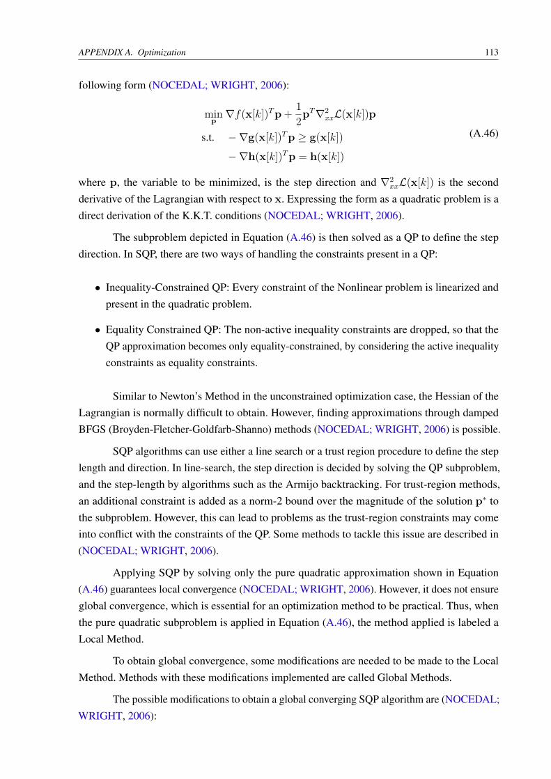
APPENDIX A. Optimization 113
following form (NOCEDAL; WRIGHT, 2006):
minp
∇f(x[k])T p +1
2pT ∇2
xxL(x[k])p
s.t. − ∇g(x[k])T p ≥ g(x[k])
− ∇h(x[k])T p = h(x[k])
(A.46)
where p, the variable to be minimized, is the step direction and ∇2xxL(x[k]) is the second
derivative of the Lagrangian with respect to x. Expressing the form as a quadratic problem is a
direct derivation of the K.K.T. conditions (NOCEDAL; WRIGHT, 2006).
The subproblem depicted in Equation (A.46) is then solved as a QP to define the step
direction. In SQP, there are two ways of handling the constraints present in a QP:
• Inequality-Constrained QP: Every constraint of the Nonlinear problem is linearized and
present in the quadratic problem.
• Equality Constrained QP: The non-active inequality constraints are dropped, so that the
QP approximation becomes only equality-constrained, by considering the active inequality
constraints as equality constraints.
Similar to Newton’s Method in the unconstrained optimization case, the Hessian of the
Lagrangian is normally difficult to obtain. However, finding approximations through damped
BFGS (Broyden-Fletcher-Goldfarb-Shanno) methods (NOCEDAL; WRIGHT, 2006) is possible.
SQP algorithms can use either a line search or a trust region procedure to define the step
length and direction. In line-search, the step direction is decided by solving the QP subproblem,
and the step-length by algorithms such as the Armijo backtracking. For trust-region methods,
an additional constraint is added as a norm-2 bound over the magnitude of the solution p∗ to
the subproblem. However, this can lead to problems as the trust-region constraints may come
into conflict with the constraints of the QP. Some methods to tackle this issue are described in
(NOCEDAL; WRIGHT, 2006).
Applying SQP by solving only the pure quadratic approximation shown in Equation
(A.46) guarantees local convergence (NOCEDAL; WRIGHT, 2006). However, it does not ensure
global convergence, which is essential for an optimization method to be practical. Thus, when
the pure quadratic subproblem is applied in Equation (A.46), the method applied is labeled a
Local Method.
To obtain global convergence, some modifications are needed to be made to the Local
Method. Methods with these modifications implemented are called Global Methods.
The possible modifications to obtain a global converging SQP algorithm are (NOCEDAL;
WRIGHT, 2006):
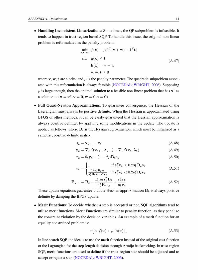
APPENDIX A. Optimization 114
• Handling Inconsistent Linearizations: Sometimes, the QP subproblem is infeasible. It
tends to happen in trust-region based SQP. To handle this issue, the original non-linear
problem is reformulated as the penalty problem:
minx,v,w,t
f(x) + µ[1T (v + w) + 1T t]
s.t. g(x) ≤ t
h(x) = v − w
v,w, t ≥ 0
(A.47)
where v,w, t are slacks, and µ is the penalty parameter. The quadratic subproblem associ-
ated with this reformulation is always feasible (NOCEDAL; WRIGHT, 2006). Supposing
µ is large enough, then the optimal solution to a feasible non-linear problem that has x∗ as
a solution is (x = x∗,v = 0,w = 0, t = 0)
• Full Quasi-Newton Approximations: To guarantee convergence, the Hessian of the
Lagrangian must always be positive definite. When the Hessian is approximated using
BFGS or other methods, it can be easily guaranteed that the Hessian approximation is
always positive definite, by applying some modifications in the update. The update is
applied as follows, where Bk is the Hessian approximation, which must be initialized as a
symetric, positive definite matrix:
sk = xk+1 − xk (A.48)
yk = ∇xL(xk+1,λk+1) − ∇xL(xk,λk) (A.49)
rk = θkyk + (1 − θk)Bksk (A.50)
θk =
1 if sTk yk ≥ 0.2sT
k Bksk
0.8sTk
Bksk
sTk
Bksk−sT ykif sT
k yk < 0.2sTk Bksk
(A.51)
Bk+1 = Bk − BksksTk Bk
sTk Bksk
+rT
k rk
sTk rk
(A.52)
These update equations guarantee that the Hessian approximation Bk is always positive
definite by damping the BFGS update.
• Merit Functions: To decide whether a step is accepted or not, SQP algorithms tend to
utilize merit functions. Merit Functions are similar to penalty function, as they penalize
the constraint violation by the decision variables. An example of a merit function for an
equality constrained problem is:
minx
f(x) + µ‖h(x)‖1 (A.53)
In line search SQP, the idea is to use the merit function instead of the original cost function
or the Lagrangian for the step-length decision through Armijo backtracking. In trust-region
SQP, merit functions are used to define if the trust-region size should be adjusted and to
accept or reject a step (NOCEDAL; WRIGHT, 2006).