john kuszczak memorial lecturecengel/publishedpapers/canadaexchangerate.pdfjohn kuszczak memorial...

John KuszczakMemorial Lecture

341

Introduction

Canada and the United States are two large economies sharing the NorthAmerican continent, but separated by an exchange rate. Should monetarypolicy stabilize the Can$/US$ exchange rate? Or does the movement in theexchange rate reflect optimal adjustment to shocks to the Canadian and USeconomies?

This paper proceeds to explore the question by:

• Examining the evolution of the “border effect” as measured by goods-price deviations between Canada and the United States. Following themethods of Engel and Rogers (1996) and Engel, Rogers, and Wang(2004), we construct a measure of the degree of integration of the USand Canadian economies. We show how this border measure has evolvedsince 1990. The apparent barriers actually rise steadily from around 1994and peak around 2001, before falling dramatically in the past few years.

• Reviewing the evidence on the determination of the Canadian realexchange rate. Amano and van Norden (1995) and Chen and Rogoff

Canada’s Exchange Rate: New Evidence,a Simple Model, and Policy Implications

Charles Engel*

* I thank Wei Dong for excellent research assistance and Mick Devereux and GiancarloCorsetti for helpful discussions. This research was supported in part by a grant from theNational Science Foundation to the University of Wisconsin, and in part by a stipend fromthe Bank of Canada.

342 Engel

(2003) estimate models that show that the Canadian dollar strengthens asthe price of commodities rises. Both papers present a model that explainsthis relationship by relating export prices of commodities to changes inthe price of non-traded to traded goods.

• Accounting for the movements in the Can$/US$ real exchange rate. Wefind that movements in the relative price of non-traded goods do notappear to explain much of the real exchange rate movement over the past15 years. But we do find that the real exchange rate tracks nominalexchange rate movements very closely. This behaviour is consistent withthe hypothesis that consumer goods are sticky in local currencies(Canadian dollars in Canada, and US dollars in the United States). Thisfinding can also explain the seemingly anomalous behaviour of the bor-der effect.

• Constructing an alternative model that might account for the behaviourof commodity prices and the Canadian dollar. In this model, the short-run impact of an increase in commodity prices works like a transfer fromthe United States to Canada. In a simple version of the model ofDevereux and Engel (2004), we find that such a transfer leads to anominal and real appreciation of the Canadian dollar.

• Examining policy implications of such a model. A number of distortionsin the economies inhabit this model. There is nominal price stickiness,and there is market incompleteness, so that it is not possible to ensureagainst fluctuations in commodity prices. We find that optimal co-operative monetary policy smoothes exchange rate fluctuations relativeto the exchange rate behaviour that would emerge if monetary policytook a neutral stance.

The evidence and the model presented in this paper are simple. They arecertainly not definitive enough that the policy implications should be takenliterally. The objective, rather, is to suggest an alternative paradigm forCanada’s “commodity currency.” The arguments of this paper at bestsuggest a role for further empirical and theoretical investigation.

1 Border Effects

If two markets for consumer goods are well integrated, prices should notdiffer greatly across the pair of markets. If formal trade barriers, transpor-tation costs, exclusivity of distribution networks, etc., are low, we might saythe markets are well integrated. Engel and Rogers (1996) (referred to as ERhereinafter) assessed the integration of Canadian and American markets forgoods by examining prices across a number of cities in the two countries.They found that the markets were, surprisingly, not very well integrated.

Canada’s Exchange Rate 343

They also discovered that the border between the United States and Canadaacted as a much larger barrier than physical distance between cities. Pairs ofcities that lie across the US-Canada border showed much less harmony inprices than city pairs within each country, even if the within-country pairswere in very distant markets. In other words, there was a large border effect.

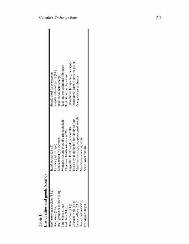
Engel, Rogers, and Wang (2004) re-examine the border effect using a newsource of data. The data are from the Economist Intelligence Unit (EIU),and they measure the prices of 97 consumer goods in 12 US cities and 4Canadian cities. The data are annual, from 1990 to 2004. EIU collects thedata to compare cost of living for cities throughout the world. The data arefor a wide variety of products. Seventy-six of the prices are for goods:41 food items, 8 clothing items, 6 consumer durables, and 21 other products.Typical items are tomatoes, ground beef, six-year aged Scotch whiskey,women’s cardigan sweater, two-slice electric toaster, and Aspirin(100 tablets). The remaining 21 items are services, such as men’s haircut(including tip) and one hour’s babysitting. Table 1 lists the products that weuse in this study.1

There are three key differences between these data and those used by ER:

(i) The goods and services in these data are very narrowly defined. ER usefairly broad categories, such as “food at home” and “men’s clothing.”

(ii) The data are not collected by a government statistical agency. The EIUdata are not nearly as well documented as official consumer price datacollected in the United States and Canada. One might suspect that theprices in this study are not as representative as those in the official data.Also, the array of goods and services is not as comprehensive as thosein the official data.

(iii) These data are actual prices. The official data used by ER are priceindexes. Price-level comparisons are not possible with index data. ERattempt to measure price deviations by looking at changes in the priceindex in one city compared with another. If the prices are equal, thenthe price changes should also be equal. But there are obvious draw-backs to this approach as a means of determining how large thedeviations from price equality are.

The empirical exercises undertaken here are very similar to those in Engel,Rogers, and Wang (2004). The chief difference is that Engel, Rogers, andWang estimate a constant border effect using panel methods for the entire1990–2002 data span. Here, we allow the border effect to vary from year to

1. In a typical year, the EIU reports prices on many more products. We use 97 items,because price data for all of them are available for each city for every year. The EIU reportsdata for various types of outlets in some instances. In all cases, we use the low-price outlet.

344 Engel

Tab

le 1

Lis

t of

cit

ies

and

good

s

US

citi

esB

osto

n,C

hica

go,C

leve

land

,Det

roit,

Hou

ston

,Los

Ang

eles

,Mia

mi,

New

Yor

k,Pi

ttsbu

rgh,

San

Fran

cisc

o,Se

attle

,W

ashi

ngto

n, D

C

Can

adia

n ci

ties

Cal

gary

, Mon

tréa

l, To

ront

o, V

anco

uver

Goo

ds (

type

of

reta

il ou

tlet

)W

hite

bre

ad (

1 kg

)D

rink

ing

choc

olat

e (5

00 g

)W

omen

’s d

ress

, rea

dy to

wea

r, da

ytim

eB

utte

r (5

00 g

)C

oca-

Col

a (1

L)

Wom

en’s

sho

es, t

own

Mar

gari

ne (

500g

)To

nic

wat

er (

200

ml)

Wom

en’s

car

diga

n sw

eate

rW

hite

ric

e (1

kg)

Min

eral

wat

er (

1 L

)W

omen

’s ti

ghts

, pan

ty h

ose

Spag

hetti

(1

kg)

Win

e, c

omm

on ta

ble

(750

ml)

Chi

ld’s

sho

es, s

port

swea

rFl

our,

whi

te (

1 kg

)B

eer,

loca

l bra

nd (

1 L

)H

ourl

y ra

te f

or d

omes

tic c

lean

ing

help

Suga

r, w

hite

(1

kg)

Bee

r, to

p-qu

ality

(33

0 m

l)B

abys

itter

’s r

ate

per

hour

Che

ese,

impo

rted

(50

0 g)

Scot

ch w

hisk

ey, s

ix y

ears

old

(70

0 m

l)C

ompa

ct d

isc

albu

mC

ornfl

akes

(37

5 g)

Soap

(10

0 g)

Tele

visi

on, c

olou

r (6

6 cm

)M

ilk, p

aste

uriz

ed (

1 L

)L

aund

ry d

eter

gent

(3

L)

Kod

ak c

olou

r fil

m (

36 e

xpos

ures

)O

live

oil (

1 L

)To

ilet t

issu

e (t

wo

rolls

)C

ost o

f de

velo

ping

36

colo

ur p

ictu

res

Pean

ut o

r co

rn o

il (1

L)

Dis

hwas

hing

liqu

id (

750

ml)

Dai

ly lo

cal n

ewsp

aper

Pota

toes

(2

kg)

Bat

teri

es (

two,

siz

e D

/LR

20)

Pape

rbac

k no

vel (

at b

ooks

tore

)To

mat

oes

(1 k

g)Fr

ying

pan

(Te

flon

or g

ood

equi

vale

nt)

Thr

ee-c

ours

e di

nner

at t

op r

esta

uran

t for

fou

r pe

ople

Ora

nges

(1

kg)

Ele

ctri

c to

aste

r (f

or tw

o sl

ices

)Fo

ur b

est s

eats

at c

inem

aA

pple

s (1

kg)

Lau

ndry

(on

e sh

irt)

Low

-pri

ced

car

(900

–129

9 cc

)L

emon

s (1

kg)

Dry

cle

anin

g, m

an’s

sui

tFa

mily

car

(18

00–2

499

cc)

Ban

anas

(1

kg)

Dry

cle

anin

g, w

oman

’s d

ress

Del

uxe

car

(250

0 cc

upw

ards

)L

ettu

ce (

one)

Dry

cle

anin

g, tr

ouse

rsC

ost o

f a

tune

-up

(but

no

maj

or r

epai

rs)

Peas

, can

ned

(250

g)

Asp

irin

(10

0 ta

blet

s)H

ilton

-typ

e ho

tel,

sing

le r

oom

, one

nig

ht in

clud

ing

brea

kfas

tPe

ache

s, c

anne

d (5

00 g

)R

azor

bla

des

(five

pie

ces)

Mod

erat

e ho

tel,

sing

le r

oom

, one

nig

ht in

clud

ing

brea

kfas

tSl

iced

pin

eapp

les,

can

ned

(500

g)

Toot

hpas

te w

ith fl

uori

de (

120

g)O

ne d

rink

at b

ar o

f fir

st-c

lass

hot

elB

eef:

ste

ak, e

ntre

côte

(1

kg)

Faci

al ti

ssue

s (b

ox o

f 10

0)Tw

o-co

urse

mea

l for

two

peop

le

(con

t’d)


Tab

le 1

Lis

t of

cit

ies

and

good

s(c

ont’

d)

Bee

f: s

tew

ing,

sho

ulde

r (1

kg)

Han

d lo

tion

(125

ml)

Sim

ple

mea

l for

one

per

son

Bee

f: r

oast

(1

kg)

Lip

stic

k (d

elux

e ty

pe)

Reg

ular

unl

eade

d pe

trol

(1

L)

Bee

f: g

roun

d or

min

ced

(1 k

g)M

an’s

hai

rcut

(tip

incl

uded

)Ta

xi: i

nitia

l met

er c

harg

ePo

rk: c

hops

(1

kg)

Wom

an’s

cut

and

blo

w-d

ry (

tip in

clud

ed)

Taxi

rat

e pe

r ad

ditio

nal k

ilom

etre

Pork

: loi

n (1

kg)

Cig

aret

tes,

Mar

lbor

o (p

ack

of 2

0)Ta

xi: a

irpo

rt to

city

cen

tre

Ham

: who

le (

1 kg

)C

igar

ette

s, lo

cal b

rand

(pa

ck o

f 20

)In

tern

atio

nal f

orei

gn d

aily

new

spap

erC

hick

en: f

resh

(1

kg)

Ele

ctri

city

, mon

thly

bill

for

fam

ily o

f fo

urIn

tern

atio

nal w

eekl

y ne

ws

mag

azin

eIn

stan

t cof

fee

(125

g)

Men

’s b

usin

ess

suit,

two-

piec

e, m

ed. w

eigh

tO

ne g

ood

seat

at c

inem

aG

roun

d co

ffee

(50

0 g)

Men

’s b

usin

ess

shir

t, w

hite

Tea

bags

(25

bag

s)So

cks,

woo

l mix

ture

346 Engel

year (extending the data to 2004) and trace the evolution of the borderbarrier.

We measure integration by estimating an equation that explains the absolutevalue of the log price difference of good i between locations j and k:

, where refers to the log of the price expressed in US dol-lars of good i in city j. All prices are expressed in US dollars so that we cancompare them across all cities.2

Following the literature that estimates the gravity model of trade, we use thelog of the distance between locations j and k, as an explanatoryvariable. ER present a simple model of how distance might also help explaindeviations from the law of one price. While ER discuss a few possiblereasons why distance might influence prices, the most plausible focuses ondistribution costs. Distribution costs are a large component of the finalconsumer price,3 and are more likely to be similar for neighbouring loca-tions. Distribution tends to be labour-intensive, and labour markets may bemore tightly integrated if they are nearer geographically.

We also use the absolute value difference in the log of the populationbetween cities j and k, , as an explanatory variable, because largercities tend to have higher prices. For the United States, the data refer toMetropolitan (MSA) Population Data. For Canada, the data are described as“Total Population, Census Div/Metro Areas.”4

A dummy variable, , which takes on the value of one if cities j and klie on opposite sides of the national border between the United States andCanada, is meant to capture the degree of integration between US andCanadian markets. The coefficient on this variable measures the absoluteaverage log price difference between US and Canadian cities that is notexplained by distance or city size (or one of the dummy variables describedbelow).

2. This means that the Canadian-dollar price of goods sold in Canadian cities is convertedinto US-dollar values by multiplying by the US dollar per Canadian dollar exchange rate.The EIU survey reports prices in US-dollar terms, converted using “the market exchangerate on the date of the survey.”3. Burstein, Neves, and Rebelo (2003) find that distribution costs account for up to 40 percent of the cost of consumer goods.4. The US data are from the Census Bureau, and the Canada data from Statistics Canada.The US data were downloaded from: <http://recenter.tamu.edu/Data/popm>, and theCanadian data from Haver in the CANSIMR database (Canadian regional economicindicators).

pi j, pi k,– pi j,

dist jk

po p jk

bord jk


We also include a dummy variable for each city, , that takes on thevalue of one if one of the cities in the city pair is city j. This variablecaptures idiosyncratic aspects of the price of a given city.

We estimate this regression for each of the 15 years in our sample:

. (1)

This equation was estimated for all the goods and services together and thenseparately for the goods and the services.

In contrast to the findings of Engel, Rogers, and Wang (2004), the estimatedcoefficients on the distance variable are rarely statistically different fromzero. The distance coefficient takes on the correct sign in 14 of the 15 years,but is statistically significant (in a one-sided test at the 5 per cent level) inonly 4 of the years. The population variable fares better. It takes on theexpected sign in 14 of the 15 years, and was statistically significant (again ina one-sided test at the 5 per cent level) in 9 of the years. Compared withEngel et al. (2004), the lack of statistical significance in these regressions isprobably attributable to the lower power of the tests when the regressions arerun year by year as opposed to as a panel regression.

But we do find that the border coefficient is of the right sign and easilystatistically significant (at the 5 per cent level) in all years. Figure 1 plots theestimated border coefficients. In the graph, we refer to goods as “tradedgoods” and to services as “non-traded goods” on the grounds that thephysical goods in our sample are easily transportable across borders, whilethe services are not. The numbers on the vertical axis can be interpreted asthe average log price deviation imposed by the border effect.

For all goods and services, and for the subset of traded goods, the bordercoefficient falls initially in the early 1990s from around 0.08 (or, roughly8 percentage points) to 0.04 for traded goods (and slightly higher for allgoods). But then, in the period from 1994 to 2001, the border coefficient fortraded goods rises back to around 0.10. Finally, between 2001 and 2004, thecoefficient falls back to about its 1994 level of 0.04. The border effect fornon-traded goods shows a nearly monotonic increase from 1990 to 2001,rising from around 0.03 to 0.17. But then between 2001 and 2004, it fallssharply to approximately 0.05.

What accounts for these fluctuations in the border effect? Did the US andCanadian economies really become less integrated during much of the

citdum j

pi j, pi k,– β1dist jk β2 po p jk β3bord jk+ +=

αhcitdumh ui jk,+h 1=

N

∑+

348 Engel

1990s? And why has there been a sudden apparent increase in integrationsince 2001? We return to these questions in section 3.

2 The Canadian Dollar andthe Commodity Terms of Trade

Here, we review empirical evidence gathered by Amano and van Norden(1995) and Chen and Rogoff (2003) that links the value of the Canadiandollar to the export price of non-energy commodities. Both papers findevidence that as the price of commodities increases, the value of theCanadian dollar strengthens (in real terms).

The studies take slightly different approaches, but reach essentially the sameconclusion. Amano and van Norden (1995) use monthly data on commodityprices from 1973Q1 to 1992Q2 to estimate an error-correction model thatrelates Canada’s real CPI exchange rate relative to the United States tocommodity prices and oil prices. In this dynamic model, they find that anincrease in commodity prices leads to a real appreciation (while,surprisingly, the effect of oil prices on the real Canadian dollar is in theopposite direction).

Chen and Rogoff (2003) revisit this relationship, using quarterly data from1980QI to 2000QI. They find a statistically significant relationship betweenthe Can$/US$ real exchange rate and the non-energy commodity price index

Figure 1Estimated “border coefficients” (1990–2004)

0.18

0.16

0.14

0.12

0.10

0.08

0.06

0.04

0.02

0.001990 1991 1992 1993 1994 1995 1996 1997 1998 1999 2000 2001 2002 2003 2004

All goods Traded goods

Non-traded goods


for some (but not all) of their statistical specifications.5 They note that therelationship between the commodity terms of trade and the real exchangerate seems to be tighter for Canada relative to its large, non-US, tradingpartners.

What explains the relationship of the commodity terms of trade with the realexchange rate? Both papers offer similar explanations. It is helpful to quotedirectly from Chen and Rogoff (2003, 149):

First, consider the following extension of the flexible-priceBalassa-Samuelson model. Let Home be a small economywhose agents consume three goods—non-traded goods,exports, and imports—but produce only the first two. Assumethat labour is perfectly mobile across industries, and thatphysical capital can be freely imported from abroad at realinterest rate r, measured in importables. The productionfunction for exportables is , where y and k areoutput and capital per unit labour, respectively, and

is the analogous function for non-tradedgoods production. Let be the world price of exportables,which is given exogenously to the small country, and bethe Home price of non-traded goods, both measured in termsof importables. Then, assuming that labour mobility leads to acommon wage across the two Home industries, one can derivethe approximate relation:

where a “hat” above a variable represents a logarithmicderivative, and and are labour’s income share in thenon-traded and export goods sectors, respectively. Thus, theeffect of a rise in the relative price of exportables is the sameas a rise in traded goods productivity in the standard Balassa-Samuelson model. The impact on the real exchange ratedepends, of course, on the utility function. Assume a simplelogarithmic (unit-elastic) utility function: .Normalizing the price of importables to one, the consumption-based consumer price index is then given by .Therefore, as moves proportionately in response to ,

5. They also examine the statistical relationship for other “commodity currencies”—ofAustralia and New Zealand. For these countries, they find that the link between commodityprices and exchange rates is more robust to statistical specification than for Canada.

yx Ax f kx( )=

yN AN f kN( )=px

pN

pN

µLN

µLX---------

Ax px+( ) AN–=

µLN µLX

U CNα C1

βC 1 α– β–( )X=

pNα p 1 α– β–( )

XpN pX

350 Engel

the effect of an export price shock on the utility-based real CPIis then given by . Assuming that importables accountfor 25% of consumption, the elasticity of the CPI with respectto a unit change in the price of exportables would be 0.75,which is broadly consistent with our estimated coefficients. (If

—it is standard to assume that non-traded goodsproduction is more labour intensive—one would get a largereffect.)

Here, we do not challenge the empirical work linking the value of the realCanadian dollar to commodity prices, but we offer evidence that themechanism linking the two does not work through the relative price of non-traded goods. We argue that the evidence on Canadian prices and theexchange rate is consistent with a view that the Canadian CPI, expressed inunits of Canadian dollars and denoted P, and the US CPI, expressed in USdollars and denoted , are sticky in their local currencies. That is,Canadian consumer prices are set in Canadian dollars and adjust sluggishly,and US consumer prices are set in US dollars and also adjust slowly. Theimplication is that the real Canadian exchange rate, given by , whereS is the Canadian dollar per US dollar exchange rate, is tightly linked to thenominal exchange rate S. Call this model the LCP (local currency pricing)model.

Section 3 presents evidence supporting this view and evidence against themodel in which the Canadian real exchange rate is driven by the relativeprice of non-traded goods. Section 4 presents an alternative model of how anincrease in commodity prices might lead to a real appreciation that is consis-tent with the data.

3 Evidence on Canada’s Real Exchange Rate

Figure 2 plots a measure of Canada’s real exchange rate based on the pricedata from the EIU, annually from 1990 to 2004. The line is denoted “pricedifference for all goods.” This line is calculated by taking ,the log of the price of good i in US city k relative to log of the price of goodi in Canadian city j, with both expressed in a common currency. We firstaverage this price difference for each good i across all Canadian/US citypairs and across all goods.

An increase in this price indicates that US consumer prices are risingrelative to Canadian consumer prices. That is, an increase reflects a realdepreciation of the Canadian dollar. Figure 2 shows that sometime between1992 and 1993, average prices became higher in the United States than inCanada (the average price difference exceeds zero). That price differential

pX1 β–( )

µLN µLX>

P∗

SP∗ P⁄

pi USk, pi CAj,–


rose until it peaked in 2001 at nearly a 30 per cent difference. Between 2001and 2004, the average price differential fell to around 10 per cent.

Figure 2 also plots s, the log of S, the Canadian dollar per US dollarexchange rate. For graphical purposes, the 1990 value of s was set equal tothe 1990 value of the relative price. The plot indicates remarkably closemovement between the real and nominal exchange rates. In log levels, thecorrelation coefficient is 0.979, and in first differences it is 0.882.

That evidence alone strongly supports the view that Canadian consumerprices are set in Canadian dollars, and US consumer prices are set in USdollars. But it is not definitive. In fact, the close correlation of real andnominal exchange rates is perfectly consistent with a world in which there iscomplete nominal price flexibility and where real exchange rates are linkedto the relative price of non-traded goods.

To see this, following Chen and Rogoff’s exposition of the classical model,let the nominal price index in Canada be given by , where isthe nominal price of non-traded goods, and is the nominal price oftraded goods. Following the model of Chen and Rogoff, is an index ofimported and exported traded goods:

,

where again the upper-case Ps refer to nominal prices.

PNα PT

1 α– PNPT

PT

PT PI

β1 α–------------

PX

1 α– β–1 α–

----------------------

=

Figure 2Relative prices and exchange rates for Canada and the United States

0.5

0.4

0.3

0.2

0.1

0.0

–0.1

–0.21990 1991 1992 1993 1994 1995 1996 1997 1998 1999 2000 2001 2002 2003 2004

Exchange ratePrice difference for traded goods

Price difference for all goodsPrice difference for non-traded goods

352 Engel

Assume that foreign consumers have a price index with identical weights.Use lower-case letters to represent prices. (To avoid confusion, I specifyhere that this notation is at odds with the notation of Chen and Rogoff above.In their model, lower-case ps represented the level of prices of goods relativeto the numeraire good. Here, lower-case ps are the logs of the nominalprices.)

We can write the log of the real exchange rate as:

. (2)

If we now use the usual assumption of the classical model (implicit in Chenand Rogoff’s description) that the law of one price holds up to a constant, sothat , where k is some constant, we obtain:

, (3)

or

. (4)

Equation (3) shows us directly that the real exchange rate should be relatedto the relative price of non-traded to traded goods in the home relative to theforeign country (Canada relative to the United States).

Equation (3) is expressed all in terms of real prices. The classical model canbe consistent with a wide variety of behaviour of nominal prices. For exam-ple, if Canadian and US policy-makers kept inflation (in local currencies)equal in the two countries, then would be constant. In that case, fromequation (3), the log of the nominal exchange rate, s, would equal the log ofthe real exchange rate, q, up to an additive constant. So, the fact that nominaland real exchange rates co-move can be consistent with the classical modelin which real exchange rates reflect movements in the relative prices of non-traded goods.

But there are two other implications of the classical model that are directlycontradicted by the data. The first is that , i.e., theassumption that the law of one price holds for traded goods (up to aconstant). Figure 2 also plots the “price difference for traded goods.” It iscalculated the same way as the “price difference for all goods,” but averagesonly across prices of traded goods. That is, it is a measure of .

It is easy to see from Figure 2 that is not constant. In fact, ittracks very closely. The correlation of these two series inlevels is 0.999. In first differences, the correlation is 0.992. As one might

q s p∗ p–+ α s pT* pT–+( ) 1 α–( ) s pN

* pN–+( )+= =

s pT* pT–+ k=

q s p∗ p–+ αk 1 α–( ) s pN* pN–+( )+= =

q s p∗ p–+ k 1 α–( ) pN pN*– pT pT

*–( )–[ ]–= =

p∗ p–

s pT* pT–+ k=

s pT* pT–+

s pT* pT–+

q s p* p–+=


expect, given these correlations, we also find that is highlycorrelated with the nominal exchange rate, s. The correlation in levels is0.978, and in differences is 0.883.

This behaviour is completely consistent with a sticky-price LCP model inwhich the Canadian price of traded consumer goods, , is rigid and presetin Canadian dollars, while the US price of consumer goods, , is set in USdollars and adjusts sluggishly.

Figure 2 also graphs the “price difference for non-traded goods,” a measureof constructed analogously to the measures of and

. From the graphs, it is easy to see that is alsohighly correlated with s, , and . In levels, those corre-lations are 0.970, 0.993, and 0.987, respectively. In differences, the respec-tive correlations are 0.816, 0.947, and 0.901.

That behaviour is again consistent with local-currency price stickiness ofand . If all consumer prices are sticky in consumers’ currencies, then

, , and will all follow s quite closely, asindeed they do in Figure 2.

Note, however, that the close correlation of with s or withis also consistent with the classical model, as equation (2) makes

apparent. What the classical model cannot account for are the movements of: its correlation with s, , and . But the

LCP model is consistent with all of the prices plotted in Figure 2.

The second major implication of the classical model that is inconsistent withthe data can be seen in Figure 3. This figure shows “price difference for non-traded goods – price difference for traded goods.” This is a measure of

. Equation (3) of the classical model says that thisrelative price should be perfectly correlated with the real exchange rate,

. There is support for the classical model, but thecorrelations are quite low: 0.340 in levels and 0.218 in differences. In fact,as is evident from Figure 3, is negatively seriallycorrelated at the annual frequency, while is positively seriallycorrelated and quite persistent.

Equation (3) not only implies that is perfectlycorrelated with q, but it also implies that is much morevolatile than q. The variance of q should be only times the varianceof , where is the weight of non-traded goods inthe price index. Clearly, the relative variances go the other way. (Thestandard deviation of is only about one-fifth thestandard deviation of q!)

s pT* pT–+

pTpT

*

s pN* pN–+ s pT

* pT–+q s p* p–+= s pN

* pN–+s p* p–+ s pT

* pT–+

pN pN*

s pN* pN–+ s pT

* pT–+ s p* p–+

s pN* pN–+

s p* p–+

s pT* pT–+ s p* p–+ s pN

* pN–+

pN pN*– pT pT

*–( )–

q s p* p–+=

pN pN*– pT pT

*–( )–s p* p–+

pN pN*– pT pT

*–( )–pN pN

*– pT pT*–( )–

1 α–( )2

pN pN*– pT pT

*–( )– 1 α–

pN pN*– pT pT

*–( )–

354 Engel

On the other hand, the low correlation of withis exactly the prediction of the LCP model, as is the low

volatility of compared to q.

If we adopt the LCP model, we are now also able to understand the borderpuzzle raised in section 1 of this paper. Why did the measured border effectrise throughout most of the 1990s, but then drop from 2001 to 2004? Theanswer is not in changing trade barriers. The answer is in local currencypricing. While some sort of barriers are needed to explain why consumersdo not arbitrage price differences across locations, it is not time variation inthose barriers that accounts for time variation in the border coefficient (asseen in Figure 1). Instead, the movements of the border coefficient seem tobe mostly related to movements in the exchange rate. As Figure 2 shows,consumer prices in the United States rose relative to those in Canada as thenominal exchange rate rose. It was not until the US dollar began todepreciate that the price gap narrowed and the border coefficients fell. Thatis, by consumer price measures, the US dollar was overvalued and becameincreasingly overvalued relative to the Canadian dollar through the 1990s.Since 2001, the US dollar has depreciated and become less overvalued.

Many recent papers6 have argued that the failures of the law of one price—the deviations of from zero—can be explained by distribution

6. Among them prominently are Burstein, Neves, and Rebelo (2003) and Burstein,Eichenbaum, and Rebelo (2004).

pN pN*– pT pT

*–( )–q s p* p–+=

pN pN*– pT pT

*–( )–

s pT* pT–+

Figure 3Relative prices and exchange rates for Canada-US

0.30

0.25

0.20

0.15

0.10

0.00

–0.05

–0.151990 1991 1992 1993 1994 1995 1996 1997 1998 1999 2000 2001 2002 2003 2004

Exchange ratePrice difference for all goodsPrice difference for non-traded goods– price difference for traded goods

0.05

–0.10


costs of traded consumer goods. The argument revives the classical modelby explaining that the measured (log) of the price of traded goods, , isactually a weighted average of the true price of traded goods as measured atthe dock, , and the price of non-traded goods and services used to bringthe traded goods to the consumer:

. (5)

We can then substitute this expression (and its counterpart for the foreigncountry) into , and amend equation (1) to write:

.

Now, according to this “revised classical” (RC) model, the law of one priceholds for traded goods at the dock, so , where k is someconstant. So we have

. (6)

At first blush, the RC model seems compatible with our data. On the onehand, we are unable to measure , because we have only data onconsumer prices and not data on true traded goods prices at the dock. So wecannot verify or disprove the assumption that the law of one price holds,

.

By analogy to the derivations above, we might rewrite equation (4), underthe assumption that , to obtain:

. (7)

But this also does not give us an equation we can verify or refute, againbecause we do not observe .

It would seem that the only equation of the RC model we can examineempirically is equation (5), which implies that is highlycorrelated with . But we have already noted that correlation ishigh. To be sure, that high correlation is also consistent with the LCP model,and also with the original version of the classical model (see equation (2))that was refuted by other evidence.

But there is evidence that we can use. Even though is not a perfectmeasure of the price of traded goods at the dock, , it does containinformation about traded prices at the dock. We can exploit the fact thatconsumer traded goods are intensive in the actual traded good comparedwith consumer non-traded goods. That is, the share of the true traded goods,

pT

pD

pT ψpD 1 ψ–( ) pN+=

s pT* pT–+

q αψ s pD* pD–+( ) 1 αψ–( ) s pN

* pN–+( )+=

s pD* pD–+ k=

q αψk 1 αψ–( ) s pN* pN–+( )+=

s pD* pD–+

s pD* pD–+ k=

s pD* pD–+ k=

q s p* p–+ k 1 αψ–( ) pN p–N*

pD pD*

–( )–[ ]–= =

pD pD*–

s pN* pN–+

s p* p–+

pTpD

356 Engel

, in the price of consumer traded goods is greater than the share of truetraded goods in consumer non-traded goods, which is zero.

So, equation (4) can be written as:

.

Substituting into equation (6), the RC model implies:

. (8)

Equation (7) gives us a relationship between the real exchange rate and sub-indexes of prices we can observe. It is exactly like equation (3) in implyingthat should be perfectly correlated with the realexchange rate, . But this was the empirical implication thatFigure 2 refutes.

Equation (3) also had the implication that the variance ofhad to be greater than the variance of .

That is not true of equation (7). can have a smallervariance if . What is the meaning of this condition? is theweight of , the non-traded distribution services, in the price of the tradedconsumer good, . is the weight of the price of traded consumergoods at the dock, , in the overall consumer price index, p. Thatcondition could plausibly be met, but recall that in our data the standarddeviation of is only one fifth the standard deviation of

. For the RC model to account for this, we would need

.

For this to be possible, the weight of in would have to be less thanone fifth.

Put another way, equation (4) implies that the standard deviation ofmust equal times the standard deviation in ,

if the classical model is correct and equals zero.7 In our data,and . For these

statistics to be consistent with the classical model, we would need

7. I thank Mick Devereux for pointing this out to me.

γ

pN pD–pN pT–

ψ-------------------=

q s p* p–+ k1 αψ–

ψ-----------------

pT pT*–[ ]–= =

pN pN*– pT pT

*–( )–q s p* p–+=

pN pN*– pT pT

*–( )– q s p* p–+=pN pN

*– pT pT*–( )–

1 ψ αψ>– 1 ψ–pN

pT αψpD

pN pN*– pT pT

*–( )–s p* p–+

ψ 1α 5+-------------=

pD pT

s pT* pT–+ 1 ψ– s pN

* pN–+s pD

* pD–+s.d . s pT

* pT–+( ) 0.107= s.d . s pN* pN–+( ) 0.115=


. That is, the actual traded content of traded goods would have tobe very small—only 7 per cent of the total value of the traded consumergood.

So the evidence works against even the RC model of the real exchange rate.A simpler explanation of these data is the LCP model. But what replaces theclassical model to explain the relationship between the price of commoditiesand the real exchange rate? Section 4 sketches a very simple LCP model,based on the work of Devereux and Engel (2004). It incorporates local-currency price stickiness for consumer goods, but potentially can explain thebehaviour of commodity currencies.

4 A Simple Model

Here, we outline a very simple model based on Devereux and Engel (2004).(This work is referred to as DE hereinafter.) The model cannot masqueradeas a realistic description of the Canadian economy. It is not dynamic anddoes not allow for any asset trade. It is a two-country model, and so it doesnot account for the determination of commodity prices in a world economyin which Canada and the United States are a part. Because the model isstatic, it is not amenable to examining the role of price adjustment. Themodel does not even account for the different sizes of the US and Canadianeconomies. But the model may contain the seed of the economics that linkscommodity prices to the real exchange rate in Canada.

Commodity prices are determined in the global economy, and not just by thesupplies and demands of the US and Canadian economies. Our approachassumes that the United States and Canada are small in the markets forcommodities—that they are price-takers.

We are concerned about the short-run effects of commodity price changeson exchange rates. The “short run” is the period during which certainnominal prices have not fully adjusted. The model presented here is one inwhich prices of consumer goods are sticky and set in the currency of theconsumer. That is, it is an LCP model, and is thus consistent with the datareported in section 3.

The model treats all consumer goods as non-traded. Final consumer goodsare assembled from traded intermediate goods. Consumer goods in eachcountry require locally produced tradable intermediate goods and importedintermediate goods. We assume that the law of one price holds for the tradedintermediate goods. We assume that intermediate goods prices are flexibleand can adjust to shocks.

ψ 0.073=

358 Engel

Commodities are separate sectors of the economies, and are modelled verysimply. In the short run, supply and demand for commodities are highlyinelastic. When the price of a commodity increases, in the short run theeconomic effect is principally an increase in wealth for the exporter and adecrease in wealth for an importer. This leads us to capture the role ofcommodity price fluctuations in the short run as a simple transfer. Whencommodity prices rise, there is a transfer from the United States to Canada.That is, there is a decrease in wealth for the importer of commodities (theUnited States) and an increase in wealth for the exporter (Canada). Giventhe confines of a two-country model, we are forced to assume that Canada’sgain is exactly equal to the US loss.

Our model is essentially the same as that of DE, except for the followingdifferences:

• DE focus on the effects of real shocks to labour supply. In our model, theonly source of shocks is to commodity prices, i.e., to the transfer.

• DE mainly examine models in which asset markets are complete. Wewill assume, to the contrary, that there is no asset trade. Given that thetransfer is the only source of shocks, what we mean is that there is noinsurance market for these transfers. That is the only missing assetmarket. If it were in place, asset markets would be complete.

• DE allow some prices to be flexible and some to be fixed, both forconsumer prices and for intermediate prices. In DE, some consumerprices are fixed in consumers’ currencies and some are flexible. Someintermediate goods prices are fixed in producers’ currencies, and someare flexible. Here, we look only at the version of the model in which allconsumer prices are set in local currencies and all intermediate prices areflexible.

• We slightly simplify household preferences, having leisure enter theutility function quasi-linearly.

• In assessing monetary policy rules, we do not consider how a change inthe rule would affect the ex ante preset nominal prices, as DE do. Thisconsideration might be important if we were considering the welfareimplications of various policies, but is not very important in consideringthe implications of policies for exchange rate smoothing.

Otherwise, the model is identical to that of DE, and their paper contains afuller exposition of the model than the brief outline contained here.

Household i in the home country has preferences given by:

, with . (9)U i( ) 11 ρ–------------C i( )1 ρ–

L i( )–= ρ 0>


C represents aggregate consumption. It is a constant-elasticity-of-substitution aggregate over a continuum of home-produced final com-modities with an elasticity of substitution of . L represents labourservices that each household uses to produce an intermediate good. Foreignhouseholds have identical preferences, but theirs are defined overconsumption of final goods sold in the foreign country and foreign labour.

Each household in the home country produces an intermediate goodaccording to the production function . Each variety of thefinal consumption good in the home country is produced using domestic andforeign intermediate good aggregates. For instance, the final good variety jis produced using the home and foreign intermediate good aggregates,respectively and , with the production function:

, (10)

where is the elasticity of substitution between the home and foreign inter-mediate goods aggregates. The home intermediate aggregate isdefined over a continuum of home-produced intermediate goods, withelasticity of substitution :

, with ,

and is defined analogously. Home households consume all of eachhome final good variety .

As noted above, we assume that all consumer prices are set in the consumercurrency. Producers of final goods will alter production levels to meetdemand. We set the price of consumer goods in each country equal to one.

We eliminate any sources of inefficiency that are due to monopoly pricingwedges in the intermediate goods sectors. To avoid these, we assume thatfirms receive a per-unit subsidy on production to ensure that price wouldequal marginal cost. The subsidy is financed by lump-sum profit taxes on theproducers.

For household/intermediate-goods producers, the first-order condition forthe trade-off between consumption and leisure is:

. (11)

θ 1>

Y H i( ) L i( )=

Y H j( ) Y F j( )

Y j( ) 12---

1γ---

Y H j( )γ 1– γ⁄ 12---

1γ---

Y F j( )γ 1 γ⁄–+

γ γ 1–⁄

=

γY H j( )

φ

Y H j( ) Y H i j,( )φ 1–

φ------------

id0

1∫

φφ 1–------------

= φ 1>

Y F j( )Y j( )

PH Cp

=

360 Engel

This extremely simple equation requires some explanation. Each householdi sells its intermediate good at the price (denominated in the homecurrency). Given that all households are identical, is the same acrossall households and equal to the aggregate price of home-producedintermediate goods, , in equilibrium. Since we assume that the nominalprice of consumer goods is set equal to one, also equals the price ofintermediate goods relative to consumption goods. Households set themarginal rate of substitution between consumption and leisure equal to thisrelative price. Given that the marginal disutility of work equals unity, themarginal rate of substitution equals , and so we have equation (10).

The decisions of foreign households are analogous to those of homehouseholds, so we have their first-order condition given by:

. (12)

Here, is the foreign-currency price of foreign-produced intermediategoods.

Demand for labour is a derived demand coming from producers of finalgoods in each country. Their demand for intermediate goods from eachcountry depends on the level of consumption of the final good in eachcountry, and the relative price of foreign to home intermediate producers,

. We can derive the demand for home labour as:

. (13)

Note that the demand for home labour coming from foreign final-goodsproducers (and hence the demand for exports of home intermediateproducers) is given by:

.

We can also derive demand for foreign labour:

. (14)

PH i( )PH i( )

PHPH

Cρ

PF* C*ρ=

PF*

SPF* PH⁄

L12---PH

γ– 12---PH

1 γ– 12--- SPF

*( )1 γ–

+

γ1 γ–-----------

C C*+( )=

12---PH

γ– 12---PH

1 γ– 12--- SPF

*( )1 γ–

+

γ1 γ–-----------

C*

L* 12--- SPF

*( )γ– 1

2---PH

1 γ– 12--- SPF

*( )1 γ–

+

γ1 γ–-----------

C C*+( )=


The balance-of-payments equilibrium condition is that the sum of transfersfrom the foreign country to the home country plus exports of the homecountry equals imports of the home country:

. (15)

is a monetary transfer, denominated here in the home-country currency.It is assumed to be a random variable. The units of equation (14) are homecurrency.

Finally, we follow DE in assuming that the instrument of monetary policymakers in each country is nominal consumption. This could be thought of asthe equivalent in the static context as control over nominal interest rates.That is, the gross nominal interest rate is equal to the expected marginalutility of a unit of currency today relative to the marginal utility of a unit ofcurrency next period. In the static model, we take expected future values asgiven. And given that all consumer prices are assumed to be fixed and equalto one in our simple model, the marginal utility of a dollar today is deter-mined by the level of consumption today. So we are assuming that C andare instruments of monetary policy makers.

When monetary policy is passive, so that C and are not responsive toshocks, from equations (10), (11), and (14), the effect of a change in thetransfer on exchange rates is immediately apparent. Equations (10) and (11)indicate that with no change in C and , and will not change withmovements in . Therefore, equation (14) tells us how movements inaffect the exchange rate.

When the home country receives a transfer ( is positive), it is able toincrease the (domestic currency) value of its imports. For a small increase in

, starting from equal to zero, there will be a drop in S—an appreciationof the home currency—when the elasticity of demand for intermediategoods is greater than one. Specifically, we have

.

This derivative is less than zero when is greater than one.

τ 12---PH

1 γ– 12---PH

1 γ– 12--- SPF

*( )1 γ–

+

γ1 γ–-----------

C*+

12--- SPF

*( )1 γ– 1

2---PH

1 γ– 12--- SPF

*( )1 γ–

+

γ1 γ–-----------

C=

τ

C*

C* τ

C* PH PF*

τ τ

τ

τ τ

dsdτ-----

τ 0=

21 γ–-----------PF

*1 γ–S

γ– 12---PH

1 γ– 12--- SPF

*( )1 γ–

+

γ–1 γ–-----------

C1–

=

γ

362 Engel

In short, a positive commodity price shock works like a wealth transfer tothe commodity exporter. Ultimately, it will increase the value of its imports.When the elasticity of demand for imports is sufficiently high, this requiresan appreciation of the currency.

5 Policy Implications

What role might policy play in this setting? There are two sources ofinefficiencies in this model. The first is that there is no market to hedge therisk of commodity price changes. Suppose that there was a perfect insurancemarket for these shocks. This would mean that no transfers take place.Equation (14) would be altered because would drop out. In that case, therewould be no shocks to the system. Even though nominal consumer pricesare sticky, that would have no meaning, because there would be no shocksthat would cause optimal prices to deviate from preset levels.

But asset markets are not complete, so the allocations that arise in thepresence of the transfer shocks are suboptimal. In fact, when monetarypolicy is passive, C and can be set at their optimal levels independent ofthe shock. But employment levels will not be optimal. As we have seen, apositive transfer leads to an appreciation of the domestic currency. Thistranslates into a decline in the relative price of foreign intermediate goods,

, since equations (10) and (11) tell us that and will notchange with movements in when C and do not change. That, in turn,implies that foreign employment will rise and home employment will fall.But when optimal insurance for commodity price shocks is in place, em-ployment would not respond to those shocks.

A second source of inefficiency is the price stickiness of the final consumergoods. As DE emphasize, when final consumer prices are sticky inconsumers’ currencies, any change in the nominal exchange rate will lead toa change in the price of consumer goods in the home country relative to theforeign country. This is potentially inefficient. An efficient allocation wouldbe obtained only when the relative price change reflects some underlyingchange in the resource cost of producing the goods.

In this simple model, the resource cost of producing home and foreignconsumption goods is identical. Identical production functions combinehome and foreign intermediates to produce the consumption good in eachcountry. Therefore, any movement in the consumption real exchange rate isinefficient.

Both of the sources of inefficient allocation point towards exchange ratemovements as the transmitter of the distortion. Here, we ask what anoptimal, co-operative monetary policy would imply for exchange rate

τ

C*

SPF* PH⁄ PH PF

*

τ C*


movements. Specifically, we consider monetary policy under commitment,in which policy-makers can precommit to changing C and in response to

shocks. We solve the model numerically.

Figure 4 plots the exchange rate that would result under optimal policychoices for values of . The horizontal axis plots the values of equal tozero and 0.033, 0.067, 0.100, 0.133, and 0.167. In this case, we set

and . The line labelled “S” plots the exchange rate underoptimal co-operative policy, while the line labelled “S-hat” plots the ex-change rate under passive policy.

It is clear from this graph that optimal monetary policy tends to stabilize theexchange rate relative to the passive case. Optimal monetary policy tends toreduce the real exchange rate distortion that occurs when nominal exchangerates fluctuate.

Figure 4 shows that optimal policy pushes the exchange rate in the oppositedirection from under passive policy. For example, when there are positiverealizations of , we find that S rises, in contrast to exchange rate behaviourunder passive policy. Optimal policy interventions push C up and downin this case. In turn, from equations (10) and (11), there is an increase inand a decline in . The relative price of the foreign intermediate good,

, falls as under passive policy, in spite of the increase in S thatoccurs under active policy. But the decline in the relative price is less thanthat which occurs under passive monetary policy. So, optimal policy also

C*

τ

τ τ±

ρ 2= γ 2=

τC*

PHPF

*

SPF* PH⁄

Figure 4Exchange rate under optimal and passive monetary policy

1.6

1.4

1.2

1.0

0.8

0.6

0.4

0.2

–0.167 –0.133 –0.1 –0.067 –0.033 0 0.033 0.067 0.100 0.133 0.167

SS-hat

0.0

γ = 2, ρ = 2

364 Engel

reduces the distortion to employment induced by changes in the relativeprice of intermediate goods.

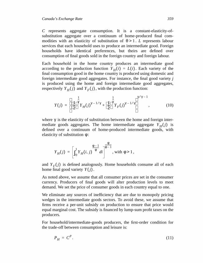
Figure 5 plots the standard deviation of the exchange rate (using thedistribution of values mentioned above) for optimal policy and passivepolicy as the coefficient of relative risk aversion, , changes. In all cases, weset . The line labelled “Se(S)” plots the standard deviation of S underoptimal policy, while the one labelled “Se(S-hat)” plots the standarddeviation under passive policy. Except for one case—when is at the veryhigh value of 10—we find that optimal policy stabilizes the nominal ex-change rate.

Figure 6 is similar to Figure 5, only we vary the elasticity of substitutionbetween home and foreign intermediate goods, , while keeping .Here, in all cases, monetary policy stabilizes nominal exchange rates.

The fact that optimal monetary policy under commitment would tend tosmooth exchange rate changes lies in contrast to the implications of theclassical model. In the classical model, the real exchange rate changesrepresent optimal movements in the relative prices of non-traded goods.Monetary policy has no role in such a model. But, Chen and Rogoff (2003)argue that there may, in fact, be a role for monetary policy to achieve theoptimal relative price adjustments when there is some nominal pricestickiness. They ask (2003, 149–50),

τρ

γ 2=

ρ

γ ρ 2=

Figure 5Exchange rate volatility under optimal and passive monetary policy

0.30

0.25

0.20

0.15

0.10

0.05

1.1 2 3 5 10

Se(S)Se(S-hat)

0.00

γ = 2, for different values of ρ


What if the price of non-traded goods is sticky? Assuming thatexport prices are flexible with complete pass-through, a simplemodel of optimal monetary policy would require the exchangerate to accommodate the requisite rise in the relative price ofnon-traded goods. This implies that the exchange rate shouldadjust one-for-one with changes in the world price ofexportables.

So there is a contrast between the implications for monetary policy of themodel presented here and the model of Chen and Rogoff. Our model impliesthat the exchange rate effects of commodity price changes should besmoothed by monetary policy.

Conclusion

The model presented here is far too simplified to give a definitive answer tohow monetary policy in Canada should respond to commodity price shocks.As we have noted, a more realistic model would be dynamic; it would(i) allow for nominal price adjustment; (ii) introduce realistic asset-marketassumptions; (iii) explicitly model the commodity market; (iv) allow for thedifferences in size of Canada and the United States; and (v) allow moregeneral functional forms for preferences and technology.

Figure 6Exchange rate volatility under optimal and passive monetary policy

0.35

0.30

0.25

0.20

0.15

0.10

1.7 2 3 5 10

Se(S)Se(S-hat)

0.05

ρ = 2, for different values of γ

0.00

366 Engel

In addition, we have not considered optimal policy from the perspective of asingle country. We have noted only the features of optimal co-operativemonetary policy in our model. But that does little to pinpoint the optimalchoices for the Bank of Canada, which does not actively co-operate with theFederal Reserve in setting interest rates.

What the model does capture is the fact that real exchange rate movementsin the short run—and it is the short run that matters for monetary policy—look more like those that occur under local currency pricing. There isanother channel through which a positive commodity shock could lead to areal appreciation in the context of an LCP model.8 It may be that thenominal exchange rate behaviour of the Canadian dollar is linked to thepolicy reaction of the Bank of Canada. A positive commodity price increaseis expansionary for the Canadian economy. It may be that the Bank ofCanada has consistently reacted to this expansion by raising interest rates,and that action, in turn, leads to the appreciation of the Canadian dollar.

It does not appear that the movements in the relative prices of non-traded totraded goods account for much of the real Can$/US$ exchange rate move-ment, at least in the short run. The actual transmission mechanism fromcommodity prices to real exchange rates matters for monetary policies.Further investigation is needed to understand the link.

References

Amano, R.A. and S. van Norden. 1995. “Terms of Trade and Real ExchangeRates: The Canadian Evidence.” Journal of International Money andFinance 14 (1): 83–104.

Burstein, A., M. Eichenbaum, and S. Rebelo. 2004. “Large Devaluations andthe Real Exchange Rate.” Northwestern University. Photocopy.

Burstein, A.T., J.C. Neves, and S. Rebelo. 2003. “Distribution Costs and RealExchange Rate Dynamics during Exchange-Rate-Based Stabilizations.”Journal of Monetary Economics 50 (6): 1189–214.

Chen, Y.-C. and K. Rogoff. 2003. “Commodity Currencies.” Journal ofInternational Economics 60 (1): 133–60.

Devereux, M.B. and C. Engel. 2004. “Expenditure Switching vs. RealExchange Rate Stabilization: Competing Objectives for Exchange RatePolicy.” University of British Columbia. Photocopy.

Engel, C. and J.H. Rogers. 1996. “How Wide Is the Border?” AmericanEconomic Review 86 (5): 1112–25.

8. Mick Devereux pointed this out to me.


Engel, C., J.H. Rogers, and S.-Y. Wang. 2004. “Revisiting the Border:An Assessment of the Law of One Price Using Very DisaggregatedConsumer Price Data.” In Exchange Rates, Capital Flows and Policy,edited by R. Driver, P. Sinclair, and C. Thoenissen. London: Routledge.

368

Robert Lafrance asked if the presumed exchange rate misalignments in thepaper were simply reflecting deviations from purchasing-power-parity (PPP)calculations. He wondered whether nominal exchange rate volatility hadmajor welfare implications, given that Canada-US PPP estimates exhibitedonly moderate volatility over time. Charles Engel responded that as nationalprices were not reflecting actual cost differences, this indicated importanteconomic inefficiencies. Nicholas Rowe argued that the data could bereconciled with a simpler model that introduced differentiated transportationcosts for goods (low) and services (high) across the border. Engel repliedthat this merited further thought, but that such a model would still requiresome form of price stickiness. John Murray wondered if this approach hadbeen tried to explain cross-border price differences with other country pairs.Engel replied no, but that it might be interesting, since the Canadian-USdollar exchange rate was not volatile when compared with other majorcurrencies. Pierre Duguay questioned the role of monetary policy in themodel, in particular, in controlling a real variable (i.e., consumption). Whatmonetary policy can actually control is a nominal variable, such as prices.Engel answered that in his highly simplified model, monetary policyultimately affects real wages and that his static model has no pricedynamics.

General Discussion*

* Prepared by Robert Lafrance.

john kuszczak memorial lecturecengel/publishedpapers/canadaexchangerate.pdfjohn kuszczak memorial...

Documents