joint abi and ima research paper, 2010...2010/03/01 · joint abi and ima research paper, 2010 4...
TRANSCRIPT

JOINT ABI AND IMA RESEARCH PAPER, 2010
DEVELOPING A RISK RATING METHODOLOGY
Report from CAMR, Cass Business School and Fathom
Financial Consulting
By Andrew Clare


DEVELOPING A RISK RATING METHODOLOGY
3
EXECUTIVE SUMMARY
The European Commission wishes to enhance the UCITS Directive and sought advice
from the Committee for European Securities Regulators (CESR). To this end CESR
published three consultation papers concerning the proposed Key Information
Document (KID) for UCITS funds.1 In these papers CESR outlined its proposals for
improving the key documentation that investors are provided with when they buy an
investment fund, and for standardising the way in which this information is presented
within the KID.
As part of these consultations CESR asked for views on the relative benefits of using a
standardised synthetic risk indicator, which provides investors with a pictorial
representation of where the risk of an individual fund sits on a scale, rather than a
narrative approach to risk disclosure. CESR has now issued its advice to the European
Commission. This paper aims to inform the ongoing debate, by assessing how to
calculate a standardised risk disclosure metric. This is extremely important, because
without a standardised approach to calculation it would be misleading for investors to
standardise the pictorial representation of risk.
This report therefore provides analysis and views on whether it is possible and/or
desirable to use a single measure of risk to categorise a wide range of investment
funds, from traditional long only funds to more complex structured products. In effect
it provides views and analysis about the appropriate empirical engine that should be
used to drive an EU-wide risk rating process. The work has three main, related
objectives:
the proposed methodology should be able to produce a rating that would be both
reliable and easily understood by non-financial experts;
it should be simple to calculate and to replicate (to avoid inconsistencies
between providers); and
it should have the potential to be applied to a wide range of investment funds
and products.
In order to assess reliability, the paper examines how successful different risk metrics
are at producing consistent risk rankings over time. This is important, because if
rankings applied to individual funds shift frequently and by large amounts, this is likely
to confuse investors and undermine the value of the risk indicator as a decision tool.
While it is difficult to forecast the level of risk from one period to another, the main
empirical findings in this report show that it is possible to forecast the relative risk
rankings of broad asset classes from one period to the next using relatively simple and
1 CESR (2009a) Consultation paper on technical issues relating to Key Information Document (KID)
disclosures for UCITS, March 2009, The Committee of European Securities Regulators, CESR/09-047. CESR
(2009b) CESR‟s technical advice at level 2 on the format and content of Key Information Document
disclosures for UCITS, July 2009, The Committee of European Securities Regulators, CESR/09-552. CESR
(2009c) Addendum to CESR‟s consultation paper on the format and content of Key Information Document
disclosures for UCITS, August 2009, The Committee of European Securities Regulators, CESR/09-716.

JOINT ABI AND IMA RESEARCH PAPER, 2010
4
largely volatility based risk measures. Of the range of risk metrics investigated in this
report, standard deviation provides the most reliable forecast of future risk rankings.
It was also found that in general, the longer the period used to calculate the risk
measure the more reliable the subsequent results. This report also argues that an
asset class based risk rating process that makes use of standard deviation as the
underlying risk metric, could also be extended to incorporate multi-asset class funds,
absolute return funds and possibly to structured products of the capital guarantee kind
too. Finally, the report argues that fund-specific details relating to each fund‟s
appropriate investment horizon, tax implications, guarantees and to fund manager-
specific risk are best dealt with in the disclosure document, and by financial
intermediaries.
In summary this report‟s main recommendations are as follows:
the risk rating engine should be based upon appropriate historic return data
spanning at least ten years to calculate a volatility-based measure of risk, as
increasing the span of the data significantly improves the stability and reliability
of the risk metric. For example, using UK smaller companies as an example, the
number of switches fell from 12 when a 3-year calculation was used to 3 when a
10-year calculation was used. In addition, unlike for the 3-year calculation, using
a 10-year calculation meant there were no switches greater than one category;
standard deviation is the best method to use to calculate the risk metric, as it
produces the most consistent rankings over time. Using standard deviation the
average correlation between the rankings for 23 asset classes and their ranking
observed in the following period was 84% - higher than for any other metric;
the risk rating process should be based upon the risks inherent in broad asset
classes, rather than on data for the returns of individual funds. This matches
existing industry practice, at least within the UK, and will facilitate the use of
longer time periods for the underlying calculation. It will also ensure a consistent
approach throughout the industry, including for new funds. The way this is
applied should give the most conservative (highest) ranking that the fund could
receive given its mandate;
despite their complexity, investment products such as absolute return funds and
some structured products should also receive a risk rating based upon the risk
mix of relevant underlying asset classes, but allowing for the impact of key
features of the fund such as leverage. Incorporating leverage in the ranking is
important because increased leverage increases risk. For example, allowing
leverage of 50% will increase the riskiness of the fund by around 50% compared
to a fund with no leverage. The calculation methodology used to rank these
funds should also be based on standard deviation. The use of Value at Risk (VaR)
would produce less consistent results, both because the forecasting ability of
VaR-based measures are worse than for standard deviation and because it would
be easy for providers with otherwise identical funds to produce different rankings
on the basis of different assumptions. The use of the fund‟s target VaR, for
example, would lead to inconsistencies, particularly without evidence that these
targets could be met consistently;

DEVELOPING A RISK RATING METHODOLOGY
5
the risk metric should be as universal as possible and therefore should not try to
capture the risks in an investment fund related to the appropriate investment
horizon of the fund, its tax implications, or any relevant manager-specific
information, like the manager‟s investment style;
the risk metric should not attempt to risk rate certain structured products,
primarily those of the enhanced income kind, because investors in these funds
have effectively insured other investors against certain financial market events.
These should be dealt with by giving them the highest risk ranking, and including
an appropriate disclosure to explain how they differ from other funds;
and finally, the risk rating process should be overseen by a committee of risk
experts that would be needed to set the broad parameters of the process and,
for example, to make judgments regarding the risks represented by any new
asset classes as they emerge. The committee should not, however, oversee the
rating of individual funds.
Overall this report provides the guidelines necessary for standardising the
measurement of risk so that it can be applied to a wide range of investment funds in a
way that will allow investors to make meaningful comparisons between one fund and
another. Achieving this is important, because ABI research shows that a good,
standardised pictorial design for explaining investment risk to consumers can increase
the number of people picking the most appropriate investment fund by over 20%, see
Driver et al (2010).
Acknowledgements
This report has been prepared on behalf of the Association of British Insurers (ABI)
and the Investment Management Association (IMA) and was used extensively in
discussions on the issues raised on risk disclosure during 2009. It is a report that has
involved considerable consultation with various individuals and groups, and it has
benefited enormously as a result of these discussions. I am grateful for the
discussions and meetings with the IMA/ABI joint steering committee for this project
and especially for the views and help of Julie Patterson, Andrew Maysey, Jonathan
Lipkin, Rebecca Driver, Yvonne Braun and Gary Brown. I would also like to thank my
colleagues at Cass Business School‟s Centre for Asset Management Research for their
comments, in particular Nick Motson, Keith Cuthbertson and Stephen Thomas. And
finally this report would not have been possible without the helpful discussions that I
have had along the way with the investment professionals at some of the UK‟s largest
insurance and asset management groups. I am very grateful to have had the
opportunity to canvas their views on the important issues addressed in this report.
However the views expressed in this report do not necessarily represent the views of
these discussants or of the two sponsoring trade bodies.

JOINT ABI AND IMA RESEARCH PAPER, 2010
6
DEVELOPING A RISK RATING METHODOLOGY
7
CONTENTS
1.0 Introduction 10
2.0 Risk 13
2.1 So what is Risk? 13
2.2 Risk Measures 13
2.3 Value at Risk 17
2.4 Fund rating, a practitioner‟s view 21
2.5 Summary 24
3.0 Empirical analysis 25
3.1 Basic data set 25
3.2 “Forecasting” methodology 26
4.0 Results 29
4.1 Full sample analysis 29
4.2 Forecasting results 32
4.3 What about VaR? 35
4.4 Summary 40
5.0 Risk bucketing 41
5.1 How do we choose the boundaries? 41
5.2 Bucket stability 43
5.3 CESR‟s suggestions for risk bucketing 46
6.0 Survey of Professionals 47
6.1 Risk ranking and „professional sense‟ 47
6.2 The survey 48
6.3 Survey results 49
6.4 Summary 52
7.0 Recommendations 53
7.1 The role for a Risk Assessment Committee 53
7.2 Single asset class funds 54
7.3 Multi-asset class funds 54
8.0 Structured products 56
8.1 Capital guaranteed notes 57
8.2 Enhanced income notes 63
8.3 CESR‟s suggestions for calculating the risk on structured products 66
8.4 Summary 67
9.0 Absolute return funds 68
9.1 What is an absolute return fund? 68
9.2 Recommendations 69
9.3 CESR‟s suggestions for calculating the risk on absolute return funds 71
10.0 Conclusions 72
A1 References 73

JOINT ABI AND IMA RESEARCH PAPER, 2010
8
A2 Earlier work on fund ratings 74
A3 Risk measures for full sample 77
A4 The risk questionnaire 79
LIST OF TABLES
Table 1 Financial market indices representing asset classes and
investment categories 25
Table 2 Full sample ranks (1987 to 2008) 29
Table 3 Correlation between full sample ranks 31
Table 4 Correlation between VaR measures with three different confidence
levels 38
Table 5 Average forecast correlations 40
Table 6 Survey-based risk rankings 50
Table 7 An intuitive categorisation 51
Table 8 The impact of leverage on a passive investment in UK equities 70
LIST OF FIGURES
Figure 1 Graphical representation of VaR 18
Figure 2 Skewed investment return distributions - Panel A: Positively
skewed returns 19
Figure 3 The volatility of the UK stock market 27
Figure 4 Average full sample ranks (1987 to 2008) 30
Figure 5 Cross plot of asset class ranking: standard deviation and downside
deviation 31
Figure 6 Rank correlation coefficients using 36 month and 12 month pre-
and post-assessment periods respectively 32
Figure 7 Rank correlation coefficients using a 36 month pre- and 12 month
post-assessment period, based on average returns 34
Figure 8 Rank correlation coefficients using a range of different pre-
assessment periods 35
Figure 9 95% VaR using full sample (1987 to 2008) 37
Figure 10 95% VaR correlations with other risk measures using full sample
(1987 to 2008) 38
Figure 11 VaR forecast results 39
Figure 12 The risk spectrum relative to cash 42
Figure 13 Risk rankings based upon subdividing the risk range into six sub-
categories 43
Figure 14 Number of category switches 44
Figure 15 Number of risk category switches using different estimation
periods 45
Figure 16 Role of respondent in organisation 48

DEVELOPING A RISK RATING METHODOLOGY
9
Figure 17 Correlation between professional ratings and risk ratings based on
risk measures 51
Figure 18 Pay-off from call option 58
Figure 19 Exposure of five year capital guaranteed note to the S&P500 index 60
Figure 20 Average exposure to the underlying index and range 61
Figure 21 Volatility of the note, its components and a credit risk free
investment 62
Figure 22 Annualised return difference between the note and an investment
in a credit-risk free instrument 62
Figure 23 The generic pay-off for writing a put option 64

JOINT ABI AND IMA RESEARCH PAPER, 2010
10
1.0 INTRODUCTION
This paper reports on work conducted on behalf of the Association of British Insurers
(ABI) and the Investment Management Association (IMA) to develop a common, single
methodology to calculate the potential risks associated with investment funds. The
work has three main, related objectives: that the proposed methodology should be
able to produce a rating that would be both reliable and easily understood by non-
financial experts; that it should be simple to calculate and to replicate; and that it
should have the potential to be applied to a wide range of investment funds and
products. This range of investments to which the methodology should be applied
spans simple long-only authorised funds to more complex, structured products.
To meet the project brief the work presented in this report had to come to views about
three important questions. The first relates to the identity of a simple and reliable risk
metric. Finance experts have been trying to measure financial market risk and in
particular its relationship with investment returns for at least fifty years. To this day
there is still no agreed or unambiguously superior approach to the measurement of
risk. Instead a wide range of risk measures exist. One of the main purposes of this
project has been to identify the most suitable risk measure from a wide range of
alternatives. Our results indicate that some very simple risk metrics are probably
reliable enough to form the basis of the metric needed to risk rank funds. However,
the empirical results presented in Section 4 of this report suggest that the most
reliable of these simple measures is standard deviation. The results also show how it
is more reliable than more complicated measures like Beta or Value at Risk (VaR).
Once this first question has been addressed, another must be dealt with, namely how
to identify a methodology that provides guidelines for the drawing of boundaries
between discreet risk categories. Although there have been many measures of risk
proposed over the years, as far as we are aware there are no specific methods for
drawing these risk intervals. The issues related to using a risk measure to categorise
funds are presented in Section 5, where the suggestion is that the full range of risk
should be sub-divided into the appropriate number of categories. The associated
empirical analysis shows that these categories are more stable the longer the period
used to measure risk. With regard to this period we suggest that it spans at least one
full business cycle.
The final question relates to the ongoing application of a predominantly quantitative
process for risk rating such a wide range and array of investment funds and products.
Financial markets are very dynamic and are likely to challenge rules devised on the
basis of historic data. How should this process be maintained over time? The
suggestion in this report is that this quantitative process be overseen by a committee,
comprised of industry risk experts who would be given the task of monitoring the
performance of the risk measure, the risk boundaries and (among other issues)
coming to views about new asset classes where necessary. The possible role of this
committee is discussed in Section 7 of the report.

DEVELOPING A RISK RATING METHODOLOGY
11
As well as dealing with these fundamental questions the report also had to deal with,
or come to a view about other important questions.
Should the risk rating process be applied at the fund level or at the asset class
level?
In designing the research agenda for this project it became clear early on in this
process that the chosen methodology should be asset class based, and not fund based.
In other words, the preferred methodology should risk rate and then rank broad asset
classes rather than offering a way of risk rating every individual investment fund or
product. This asset class based risk rating could then be used to rate all funds, since a
significant proportion of their risk will be dependent upon the asset classes in which
they invest.
This approach has a number of advantages over a fund or product based approach.
First, much longer historic data are available for asset classes (as represented by
financial market indices) than for individual funds. Thus the risk rating could easily be
based upon data that spanned more than one business cycle. Second, using asset
class data as the basis for the risk rating would make it relatively straightforward to
risk rate new or relatively new funds. Third, this approach strips out the somewhat
unpredictable element of fund manager performance, which would exist if individual
fund or product data were used. Fund managers change over time, and their
performance varies from period to period too. Fourth, discussions with a number of
fund management organisations conducted as background research for this report
revealed that the basis of their risk rating methodology was in fact the risk inherent in
asset classes. The approach proposed here is therefore already embedded in current
market practice. Finally, such an approach would be relatively simple to apply to
multi-asset class funds too.
Should the risk measure take account of the investment horizon of the
investor?
There will naturally be an important link between perceptions of risk and the
investment horizon of each, individual investor. For example consider an investor that
is saving for their retirement in thirty year‟s time. Arguably investing all of their funds
in a “low risk” asset class like cash would be more risky than investing it all in a
“higher risk” asset class like equity. In nominal terms and even in real terms, the cash
investment over thirty years would almost certainly be less volatile and would
experience fewer (if any) daily or monthly losses. But it might still be considered to be
a more risky investment strategy if the desired value of the investment in thirty year‟s
is relatively high. In other words, it is perhaps not the uncertainty relating to the
value of the investment from month to month over the thirty year period that would
be of most concern to this investor, but instead the dispersion of the value of that
investment at a particular point in the future around the target, or desired value of the
investment. In this sense, although equities may be expected to produce a more
volatile return experience for the investor from month to month, if the average return

JOINT ABI AND IMA RESEARCH PAPER, 2010
12
is higher than the average return on a cash investment then there may still be a
greater chance of the investor achieving their ultimate investment goal. Investors
may be more concerned about the dispersion of investment returns on the date that
they require the funds, than they are about the dispersion of returns over time as they
approach this date. To deal with this issue researchers have developed measures of
risk that focus on the dispersion of what they refer to as „terminal wealth‟, that is the
value of the investment portfolio at some pre-determined endpoint.
While this approach to thinking about risk is certainly very valid, we do not use it here.
This is because to do so we would need to specify an investment endpoint and a target
level of return for a „representative‟ investor. The aim of this project is not to provide
a risk rating for every investment product, for every investor, each with their own
investment horizons and objectives. Instead the aim is to produce a risk rating for one
asset class relative to another. In the view of this report the issues surrounding the
investment horizon of an investor are best dealt with by financial advisors and within
fund disclosure documentation.
Should the risk measure incorporate the tax implications of the fund?
Finally, there is a wide variety of investment products available to investors. As well
as giving investors access to the risks inherent in particular asset classes many have
been designed to increase the investment returns net of tax. These opportunities
generally exist because governments and regulators often try to encourage savings by
offering incentives through the tax system. However, the tax advantages of such
incentives may depend upon the investor‟s wealth or earnings, or even age. The work
presented in this report concentrates on gross of tax asset class returns. Once again
then, in the view of this report the tax position of an individual investor is best dealt
with by financial advisors and within fund disclosure documentation, rather than within
the risk metric.
The remainder of this report is organised as follows. Section 2 discusses the concept
of risk and explores some of the different risk measures available; Section 3 outlines
the data and methodology used in the empirical part of the report, while Section 4
discusses the main results. Section 5 addresses the issue of “risk bucketing” that is,
the process by which we categorise each asset class into a risk category, while Section
6 describes the results of a survey of risk professionals with regard to their views on
the risks inherent in a range of asset classes. Section 7 contains the main
recommendations of the report for single and multi-asset class, „long only‟
investments. Sections 8 and 9 deal with the issues surrounding the application of the
proposed methodology to structured products and absolute return funds respectively.
Finally, Section 10 outlines the main conclusions of the report, and in particular details
the arguments in favour of combining the quantitative approach proposed here with an
independent risk assessment committee.

DEVELOPING A RISK RATING METHODOLOGY
13
2.0 RISK
2.1 So what is Risk?
Risk is a nebulous concept. The Oxford English Dictionary describes risk as “a situation
involving exposure to danger; the possibility that something unpleasant will happen;
or the possibility of financial loss.” In the context of this report, investing exposes one
to the danger of financial loss that one would regard as an unpleasant experience in
the event that the loss materialised.
Economists think of risk as being the possible dispersion of future outcomes around an
expectation of that outcome. For example, we might expect a return of 10% next year
from an investment in an equity market, but the actual return on the equity market
might be much higher than 10% or indeed much lower. When investors are
particularly uncertain about the likelihood of an expected outcome it means that they
expect the possible dispersion of outcomes around the expectation to be very wide. In
other words, investors may expect a return of 10% but might also foresee a situation
where there is an equal, albeit low possibility, that the actual return turns out to be as
low as -10%. Conversely when investors are less uncertain the expected dispersion
will be lower and more “bunched” around the expectation.
2.2 Risk Measures
The oldest framework for thinking about risk has its roots in the work of Markowitz
(1952). In this work the volatility of an asset‟s historic return around its average
return over the same historic period is used as the proxy for risk. The standard
deviation of an individual asset, a market, a fund, or any combination of assets can be
calculated as follows:
1/2n
1t
2
iiti RR1n
1sd
(2.1)
where Rit is the return on asset/fund/market i in investment period t, n is the number
of investment periods over the full investment period and iR is the average return
over the full investment period.
Standard deviation measures the dispersion of returns around the average return, iR .
The idea is quite simple, those asset classes or funds that have returns that vary
greatly over time will have returns that are commensurately widely dispersed around
their mean. The greater the dispersion, the greater investor uncertainty will be about
the actual return they can expect from one period to the next. If risk can be

JOINT ABI AND IMA RESEARCH PAPER, 2010
14
characterised as uncertainty about future outcomes then in this sense standard
deviation (or variance) is a very natural representation of risk. This is arguably why
this measure is still widely used by academics, investors, investment advisors and fund
managers today.
An alternative and simpler measure is Range. This can be calculated as the difference
between the maximum and minimum return achieved by an investment over a certain
investment period. This is a measure of the maximum dispersion of return over this
period, rather than a standardised measure of the dispersion (standard deviation) that
takes into account all returns over the period. Nevertheless for some investors it
might be a suitable proxy for, or representation of risk. And it is certainly very simple
to calculate:
iii return MinreturnMax Range (2.2)
where Max returni and Min returni represent the maximum and minimum return
respectively experienced during a single investment period on asset i over the same
period, for example, the highest return in a single month minus the lowest monthly
return, if monthly data are used. The implication is that the larger the value the
greater is the risk associated with the investment.
A simple extension of Markowitz‟s framework was suggested by Sharpe (1964). This
measure is known as the Sharpe Ratio (SR) and today it is in widespread use in the
finance industry. The ratio is shown below:
i
fi
isd
RRSR
(2.3)
where fRis the average return on a “risk free” asset. The higher the average return
over and above that return that could have been earned without risk, the better.
However, if that return is earned at the expense of higher risk, represented by the
standard deviation of the return, then the investor would have simply “paid” for the
higher return by taking on greater risk and uncertainty. As such, it can be thought of
as representing a measure of the additional return achieved per unit of risk assumed,
or alternatively as a reward to risk ratio. Other things equal, the higher the Sharpe
ratio, the higher the additional return for a given unit of risk.
Another measure of risk, which is also rooted firmly in Markowitz‟s original work, is
Beta. Sharpe (1964) extended Markowitz‟s work by developing a model known as the
Capital Asset pricing Model (CAPM). Although the derivation of the model is relatively
complicated, its main conclusion – that a coefficient referred to as Beta can describe
the risk represented by all risky investments – is relatively simple. Beta (β) can be
estimated for an investment by calculating the covariance between the return on the
investment in excess of a riskless return and the return on “the market” in excess of
the same riskless return. This covariance is then divided by the variance of the excess

DEVELOPING A RISK RATING METHODOLOGY
15
return on “the market”. An investment that is estimated to have a beta equal to 1.0 is
said to be, on average, as risky as the market; while an investment with a beta of less
than 1.0 would be categorised as being less risky than the market on average; and
one with a beta greater than 1.0 would be seen as being riskier than the market. The
following expression shows how beta is constructed:
)RVar(
)R,RCov(β
m
mii ~
~~
(2.4)
where iR~
is the return on investment i in excess of the risk free rate; mR~
is the return
on the market in excess of the risk free rate; and Cov and Var represent the terms
covariance and variance respectively.
The key issue with regard to Beta is the choice of “the market”. In theory the market
should comprise all investments, but in practice the industry tends to use a broad
equity market index like the S&P500 or the FTSE-A All Share index as the proxy for the
market return. As such, the higher the covariance between the investment and the
broad equity market the greater the measured risk. The main issue with regard to
using Beta as the standardised measure of risk on investment funds is then the
definition of “the market”.
The Treynor ratio, another measure of fund risk which is very similar in spirit to the
Sharpe ratio, is based upon the idea of Beta. The expression for the Treynor ratio, TP,
is given as:
P
fPP
β
RRT (2.5)
where PR is the average return on the portfolio or the investment over a given
period; fR is the average return from a risk free asset over the same period; and P is
the fund‟s “beta coefficient”. As with the Sharpe Ratio, the average return from a risk
free asset is subtracted from the average return on the investment because the
difference between the two represents the reward for risk taking. The higher the
fund‟s beta, other things equal, the lower the Treynor ratio and the worse the fund‟s
risk-adjusted performance.
The CAPM remains the benchmark factor model of risk and return. By factor model we
mean that there is a variable that helps to “explain” the relationship between risk and
return. The CAPM has only a single factor, but other models have more than one
factor. Most notably the Arbitrage Pricing Theory attempts to map expected returns
according to a set of systematic risk factors that are normally interpreted as

JOINT ABI AND IMA RESEARCH PAPER, 2010
16
macroeconomic variables. Researchers and practitioners often use a three factor
model developed originally by Fama and French (1992) and which can best be
described as an empirical version of the CAPM. More recently the factor modelling
approach to quantifying risk has been extended to hedge funds where the number of
factors have been increased to take account of the leverage that such funds use in
generating their returns and the derivatives that they also use which is part of this
leverage.
However, these factor models are not without their critics. While they have been
shown by some to capture the risk return relationship in an economically sensible way,
other authors have demonstrated that their conclusions are neither stable over time
nor across different markets, while others have questioned their theoretical bases.
2.2.1 Downside risk
Classical measures of risk like standard deviation in effect assume that investors are
as concerned about experiencing a return that is greater than their expectation as they
are about achieving one that is lower than this expectation because they give equal
weight to both up and downside risks. However, more recent work by economists and
psychologists (see Tversky and Kahneman (1991)) suggests that investors (people)
are less concerned about receiving returns that are greater than they expect, but
instead are much more concerned about those occasions where their return turns out
to be less than they had expected, or desired. To deal with this issue today
investment professionals frequently use risk measures that concentrate only on those
occasions where investment returns are lower than a measure of the expectation of
that return. These measures of risk concentrate on what investment professionals
refer to as “downside risk”.
Perhaps the simplest downside risk measure is maximum drawdown. This measure is
the lowest return achieved over an investment horizon, in any given month during that
period if monthly data are used, or on any given day if daily data are used etc. It
essentially represents the worst historic monthly, weekly, or daily return on an
investment. It is therefore also very simple to calculate.
A slightly more complicated measure of downside risk is downside deviation (dd). It is
very closely related to standard deviation, and can be calculated as follows:
1/2n
1t
2
iti MAR(R min1n
1dd 0 ), (2.6)
Unlike standard deviation, downside deviation only takes account of returns that occur
below a certain threshold, referred to as the minimum acceptable return (MAR). On
those occasions when the return is above this MAR, in other words when the
investment has returned more than was deemed „acceptable‟, then that return

DEVELOPING A RISK RATING METHODOLOGY
17
observation is set to zero; essentially it is ignored in the risk calculation. In practice
the MAR can be set to any value. When it is set to zero it means that the measure
only looks at the dispersion of negative returns achieved by the investment2.
An extension of downside deviation is the Sortino Ratio (Sort R). This is similar to the
Sharpe ratio, where the numerator is downside deviation rather than standard
deviation and is often calculated as follows:
i
fi
idd
RRR Sort (2.7)
As with the Sharpe ratio, the higher the value of the Sortino ratio the better because it
means the higher the return achieved for each unit of risk assumed. This measure,
however, only takes into account “bad” dispersion, in other words only those occasions
where investor wealth falls, either in absolute terms or relative to a safer investment
option.
2.3 Value at Risk
Finally, the fund management industry now makes extensive use of VaR – Value at
Risk. As a measure of risk, VaR began life in investment banks as a way of
summarising the complex and interrelated risks embodied in the trading positions of
these banks, in one single number. VaR which was introduced by JP Morgan in the
1980s, is a methodology that attempts to summarise the risk of an investment
portfolio or even an entire institution. The basis of VaR can be encapsulated in the
following statement:
“We are X% certain that we will not lose more than Y pounds within the next N days”
The value Y in the statement is the “value at risk” expressed simply in monetary
terms; and X% is the level of “confidence” that we attribute to a loss equal to or
greater than Y. Although this sounds complicated it can be represented easily with a
simple graph:
2 In the empirical work in Section 4, we set the MAR equal to zero.

JOINT ABI AND IMA RESEARCH PAPER, 2010
18
Figure 1 Graphical representation of VaR
Source: Cass Business School and Fathom Research
Figure 1 shows the distribution of gains or losses expected from a particular
investment, or set of investments. In this representation the investment outcomes are
expected to conform to a normal distribution which, among other things, implies that
these gains and losses are symmetric around the mean so, ex ante, there is the same
probability of achieving a large gain, or large loss of equal magnitude. The area under
the distribution to the left of the vertical line at the VaR limit is equal to the X% in the
statement above.
Let us suppose that X%=5%, that the VaR value at this point is -£10m and that the
investment period, N, is set equal to 1 year. By saying that the VaR of the investment
is £10m with 95% confidence, we are saying that only on one in twenty occasions
would we expect the loss on the investment to be greater than £10m over the next
year. Clearly the larger the VaR, for the same initial investment value, the greater the
possible loss and the greater the risk inherent in the investment.
VaR is popular because it puts a monetary value on the risk embodied by an
investment. For most investors this is more meaningful than saying, for example, that
the standard deviation of returns on an investment over one year is 20%. It is also
popular because it focuses on that part of investment uncertainty that concerns
investors most – the potential for loss. However, VaR does not tell us necessarily how
large the loss will be in the event that the VaR limit is breached.
-20% -16% -12% -8% -4% 0% 4% 8% 12% 16% 20%
(100-X)%
Loss GainVaR

DEVELOPING A RISK RATING METHODOLOGY
19
2.3.1 A question of distribution
The representation of VaR in Figure 1 assumes that the investment outcomes are
normally distributed. But investment class returns may not be distributed
symmetrically. For example in practice there may be a greater chance of large
negative outcomes, in other words the distribution of outcomes may be “skewed” to
the left. In the event that the true future distribution of returns are skewed – either
positively or negatively – the investment‟s value at risk will be lower in the former
case and greater in the case of the latter. Figure 2 shows two different distributions.
Panel A shows a return distribution that has experienced proportionately more positive
than negative returns: the distribution is positively skewed. Panel B represents a
return distribution on an investment that has experienced more negative than positive
returns: in this case the distribution is negatively skewed.
Figure 2 Skewed investment return distributions - Panel A: Positively
skewed returns
Source: Cass Business School & Fathom Research
Figure 2 shows clearly that the VaR for the distribution that is negatively skewed is
much larger than for the VaR of the positively skewed set of returns. A larger
proportion of the returns in Panel B are worse than -1.0% compared with the
positively skewed distribution shown in Panel A. The VaR for the investment shown in
Panel A is therefore lower, because there has been a lower occurrence of negative
returns and therefore, based upon historic experience, the investor potentially stands
to lose less money compared with investments whose returns have been more
negatively skewed in the past.
0
10
20
30
40
50
60
70
-2.00% -1.00% 0.00% 1.00% 2.00% 3.00% 4.00% 5.00%
Fre
quency
Lower proportion of returns
below -1.0% compared with
Panel B
0
10
20
30
40
50
60
70
-0.06 -0.05 -0.04 -0.03 -0.02 -0.01 0 0.01 0.02 0.03
Fre
quency
Greater proportion of returns
below -1.0% compared with Panel
A

JOINT ABI AND IMA RESEARCH PAPER, 2010
20
So when risk analysts calculate the VaR of an investment, or set of investments, what
assumptions do they make about the possible distribution of these future returns?
There are two basic approaches to this issue. First, risk managers may use the
historic distribution on asset returns as an estimate of how these returns may be
distributed in the future, such as the ones shown in Figure 2. Second, they may
assume that the returns on an investment will conform to a specific distribution that
can be written down in the form of a mathematical formula3. Finally, VaR can be
calculated by looking at the past history of returns and then choosing, for example, the
fifth worst return from a set of 100 return observations, or the fiftieth worst return
from a set of 1000 observations. In both cases this observation would be taken to
represent 95% VaR of the investment, since only 5% of the outcomes were worse than
this one, by definition. The 99% VaR would be the worst return experience in a set of
100, or the tenth worst in a set of 1000 return observations, etc.
In practice there are many variations of these three broad approaches to the
calculation of VaR, probably as many variations as there are risk managers calculating
VaR.
Although one of the main attractions of VaR is that the measure accounts for the fact
that returns may not be normally distributed, practitioners often use a simple formula
that can be used to transform a VaR number into a “volatility number” (although to
some extent this defeats the object of calculating the VaR based upon the full
distribution of investment returns).
The VaR for any return series can be calculated as follows:
VaR = W(µ – Zc x σ) (2.8)
where W is the initial value of the investment, µ is the expected (or average) return on
the asset class or portfolio, Zc is the critical value4 from the normal distribution and σ
is the standard deviation of return. If we rearrange the formula we can see how a
standard deviation value can be arrived at:
σ = [VaR – (Wµ)] / (W x Zc) (2.9)
So if we can use the historic average return as a proxy for µ and if returns are
normally distributed then we can easily transform a VaR measure to a measure of
standard deviation. If not however, then the transformation will not be valid and could
lead to a misleading conclusion about the actual value at risk.
3 The normal distribution can be represented mathematically, but there are many other types of distribution
that can also be written down mathematically.
4 Zc is simply a number that allows us to identify the VaR value that we are interested in. Its value can be
found in standard statistical tables. For example, if we are wish to identify the 90% VaR we use 1.65, but if
we want to identify the 95% VaR we use 1.96.

DEVELOPING A RISK RATING METHODOLOGY
21
2.4 Fund rating, a practitioner‟s view
Historically, parts of the industry, particularly in the US, were sceptical about the
benefits of providing a standardised risk measure. In 1995 Stevens and Lancellotta5
reported on the views of a Committee set up to consider, how risk disclosure might be
improved for US mutual funds and to report the US mutual fund industry‟s views to the
SEC, the US regulator. After almost a year‟s worth of consideration of the issue of
risk disclosure, the committee recommended three main ways of improving the quality
of risk disclosure. First, that the risk of a fund‟s portfolio be considered rather than
the risk of individual securities within the portfolio. Second, that all prospectuses
should contain a bar graph showing the fund‟s total annual return over each of the
past ten years. And third, that funds should have a stated maturity policy. But of
more relevance to this project is the committee‟s view with regard to calculating and
communicating the risk on each fund, using any measure of risk. The committee
concludes:
“The Institute adamantly opposes [the author‟s emphasis] any
requirement that funds report a single, standardised numerical risk
measurement. Fundamentally flawed, this approach erroneously
assumes that a single, optimal yardstick of investment risk exists;
ignores that risk is multifaceted, necessarily having different meanings
for different investors; and poses the significant danger that investors –
neither understanding the limitations of some government-sanctioned,
all-purpose risk measure nor accurately assessing its relevance and
appropriateness to their particular circumstances and investment
objectives – nonetheless will rely on it to their detriment.”
The view of the US mutual fund industry (at least in the mid-1990s) was clear; they
were “adamantly opposed” to one of the main goals of the European Commission‟s and
CESR‟s proposals.
To get a better understanding of the views and risk rating practices of UK-based
investment product providers a number of discussions took place with some of the
UK‟s largest providers of investment funds. These interviews and discussions revealed
both broad similarities in the approach to risk disclosure, but also some very specific
differences too.
2.4.1 The views of UK investment product providers
The managers consulted operated across the full spectrum of business models. Some
sold their funds via high level financial intermediaries only, while at the other extreme
some sold directly to the general public. To some extent the distribution model
influenced the risk rating processes used, or at least how it was communicated.
However, one common feature of the risk rating methodology was that they all
5 Improving mutual fund risk disclosure, Investment Company Institute Perspective, November 1995.

JOINT ABI AND IMA RESEARCH PAPER, 2010
22
seemed to focus specifically on communicating the risks in their funds rather than on
prospective return. In other words, the ratings were not return ratings, but were
instead rankings of the perceived relative risk of each fund. However, having said this,
implied in the risk rating was the following basic principle “on average, the higher the
risk the higher the potential for realised return”.
Another common feature of their risk rating approach was the use of a measure of
historic volatility. These approaches ranged from simple volatility-based calculations,
such as standard deviation based upon monthly return data of anything up to ten
years, to the use of VaR and other monte carlo-based simulation exercises. However,
whatever the approach the initial emphasis in the rating process was on the risk
represented by broad asset classes calculated by using data on representative financial
market indices. Using this information funds and investment products were then
generally placed in to the risk category that best corresponded to its underlying asset
class. The number of risk categories used to convey degrees of risk varied from
between six to ten (their graphical representation varied greatly too). But „cash‟ was
always ranked as the least risky while asset classes such as „emerging market equities‟
were generally ranked as being the most risky.
In terms of the basic approach to risk ranking there existed a fair degree of similarity,
most seemed to base their rankings upon the underlying risk (volatility) of the broad
asset classes from which the funds derived their returns. However, there appeared to
be no general agreement with regards to how the boundaries were drawn between one
risk category and the next. Unlike the calculation of risk itself where there seemed to
be an implicit agreement that historic volatility of broad asset classes should form the
basis of the assessment of risk, I was unable to identify any agreed systematic,
quantifiable rules that established where the boundaries between one category and the
next lay. Instead, managers assessed the risk inherent in each asset class using their
chosen volatility based methodologies, and then applied judgement with regards to the
stratification of these asset classes and the boundaries between each risk group. The
lack of consensus here arguably poses the main difficulty in constructing a
standardised approach to this issue, not because each manager is so wedded to their
own approach, but instead because no obvious set of rules exist.
Finally, although the risk rating approach of each fund manager was essentially
quantitative, all the managers applied some degree of judgment to the final risk
ordering of the asset classes. Two asset classes posed particular difficulties – UK
property and high yield bonds. The strict ordering of these two asset classes based on
purely quantitative approaches did not accord with the managers‟ view of their relative
risk.
UK property as an asset class has posed a problem for two reasons. First, the strong
performance of the market until recently, meant that it began to look „fully valued‟.
This in turn meant that the perceived return upside for this asset class was low and
conversely that the perceived downside was large, particularly once the economic cycle
turned decisively in late 2007. Second, the constituents that comprise the indices
used to proxy for commercial property investment are not valued like the components

DEVELOPING A RISK RATING METHODOLOGY
23
of other financial market indices. Commercial property prices are only updated on an
infrequent basis and so the volatility of the index based upon them tends to be low.
The long economic expansion, especially in the UK, and the history of monthly
percentage changes of the property index data meant that investment professionals
did not believe that the index adequately reflected the risk represented by an
investment in commercial property. Over some time periods property index data was
not much more volatile than indices representing cash returns. Using a purely
quantitative approach to rank commercial property then might have led to it being
risk-ranked alongside cash.
High yield is a relatively new asset class in Europe, and the data available on the
market covered an economic period that, while not devoid of defaults, was fairly
benign for credit risky entities. As such the high income from these securities and
favourable economic background led to high yield indices having relatively low levels of
volatility; over some periods lower than government bond indices. Again, using a
purely quantitative approach might have led to high yield bonds being ranked below
government bonds in any volatility-based risk scale.
In both of these cases, and presumably in others in the past, managers overrode the
quantitative analysis to raise both the commercial property and high yield asset
classes to higher risk categories than were implied by measures of historic return
volatility alone.
Absolute return and structured products
One of the original objectives of this project was to establish whether it was possible
and/or desirable to use a risk rating methodology that encompassed both traditional,
long-only investment funds and also absolute return and structured products too.
First, those managers that were consulted and that offered absolute return funds all
made the point that absolute return funds are not an asset class (just as hedge funds
are not an asset class). An absolute return fund is instead just a way of managing an
asset class, or classes. The managers of absolute return funds use a variety of
investment strategies including “pairs trading”, strategies involving derivative
instruments and also leverage. All these strategies are designed to increase the return
on the fund while simultaneously reducing its risk when applied to particular asset
classes. Because of this managers tended to use the main asset class of the fund as a
starting point for determining its risk profile. However, given the nature of the
investment strategies, and in particular the use of leverage, the risk inherent in the
asset class was seen as representing the base level of the fund‟s risk profile.
Second, most managers that were consulted in the course of this project agreed that it
would be difficult to fit structured products into a risk rating continuum that included
traditional, long only investment vehicles. One of the issues was the sheer diversity of
these products. But the more important issue was the optionality embedded in the
products. However, a distinction was drawn between two broad categories of
structured product – those that can be termed as “capital guaranteed” and those that

JOINT ABI AND IMA RESEARCH PAPER, 2010
24
can be termed as “enhanced income” products. Capital guarantee varieties essentially
involve the investment in a zero coupon bond and the simultaneous purchase of a
long-dated call option, usually on an equity index, or basket of equities. The enhanced
income products usually involve the purchase of a coupon paying bond and the
simultaneous sale of put option(s) to enhance the income, usually on equity indices.
There was broad agreement that it might be possible to encompass the former into the
risk scale, but not the latter.
2.5 Summary
This section of the report has considered some of the main issues involved in risk
rating investment funds (or indeed any investment product). The following provides a
summary of the main points:
There are many ways of measuring risk that, ex ante, may be equally as good as
one another. Within the academic community there is no agreement about
which is the “best” measure of risk.
Industry practice is to risk rate investment funds not to rate them based upon
their potential for return.
Fund managers generally work to establish the risk that they believe to be
inherent in broad asset classes rather than on individual funds. Funds and
products are then „fitted into‟ the asset class risk spectrum.
The way in which managers assess asset class risk varies greatly, but the
methodologies are generally based upon measures of historic volatility. The
results in terms of risk ordering seem to vary less.
Fund managers will use their discretion based upon their professional expertise
to adjust the risk order of asset classes that seem to be „out of line‟.
There is no clear consensus on how to group asset classes into risk buckets or
where to draw the boundaries between the categories, and it is perhaps here
that there could be the greatest diversity of approach towards the risk disclosure
between one company and the next.
Managers generally believed that absolute return funds should be seen as a
strategy applied to an asset class(es) and that they should be rated accordingly;
while it was generally felt that structured products should be treated separately,
particularly those of the enhanced income variety.

DEVELOPING A RISK RATING METHODOLOGY
25
3.0 EMPIRICAL ANALYSIS
In this section of the report we introduce the data set that is used to investigate the
stability and reliability of the risk measures discussed in Section 2.2. We also outline
the chosen methodology in this section.
3.1 Basic data set
The data set comprises financial market indices and combinations of those indices, that
have been chosen to represent the range of funds available to UK investors. All the
returns data derived from the indices are in sterling terms6. Although the data set has
been chosen with a UK focus the results should be applicable to other sets of
representative investments in other currencies too. In other words these indices
simply represent a convenient set with which we can experiment.
Table 1 Financial market indices representing asset classes and investment categories
ABI sector Index proxy
Defensive* 20% Equity, 80% Bond
Cautious* 40% Equity, 60% Bond
Balanced* 60% Equity, 40% Bond
Flexible* 95% Equity, 5% Bond
UK all companies FTSE All Share index
UK smaller comps FTSE Small Cap index
UK equity income MSCI UK Value Index
Global equities DS Developed markets index
Europe excl UK DS Europe ex UK index
North America DS North American index
Asia Pacific excl Jap DS Asia ex Japan index
Japan DS Japan index
Emerging equities MSCI Emerging Markets index
UK Gilts FTA British government fixed all stocks index
£ fixed interest Barclays investment grade credit index
Sterling long bond DS benchmark 30 yr gilt index
Global fixed interest JP Morgan Global govt bond index ex UK
6This set of indices represents just one convenient categorisation that is used for the purposes of illustration.
Although the range of representative investments is fairly wide, from cash to private equity, they are not
necessarily intended to represent the definitive set of investment funds available to investors.

JOINT ABI AND IMA RESEARCH PAPER, 2010
26
Global high yield Merrill Lynch High Yield index (BB)
UK direct property IPD total return index
Property securities DS Investment trusts property index
Money market JP Morgan Global cash index
Commodities/energy S&P GSCI Commodity index
Private Equity DS Investment trusts private equity index
Note: *For the “equity” portion of these categories the FTSE All Share index was used, while the “bond” portion
was represented by the FTA British government fixed all stocks index.
The main problem involved in putting together such a set of representative indices is
the span of the data available. To undertake any meaningful risk assessment requires
data that spans as many business cycles as possible. The set of indices used to proxy
for the investment categories therefore reflects the need to identify a start date that
was as far back as possible, while at the same time leaving a suitable cross-section of
asset classes for the empirical work. The set of representative asset classes (or
sectors) along with the indices chosen to represent them are shown in Table 1.
The indices used to proxy for investment in broad asset classes described in Table 1
have all been constructed with a UK, or sterling-based investor in mind. For the
purposes of investigating the stability of different risk measures this choice should not
matter. However, in the event that a pan-European approach to this issue is adopted,
the risk analysis will have to be undertaken in each relevant currency. For example an
investment in a currency unhedged portfolio of European (ex UK) equities will
represent a different risk for a sterling-based investor compared to a Euro-based
investor. The asset class proxies simply have to be currency adjusted appropriately.
3.2 “Forecasting” methodology
The main question that is addressed in the empirical section of this report relates to
the stability and reliability of each risk metric. There exist many statistical models that
attempt to forecast financial market volatility from one period to the next. Figure 3
shows how difficult a task this is. It depicts the volatility of the UK stock market going
back to the mid-1960s, represented here by the FTSE All Share Index. Volatility can
increase or decrease from one period to the next quite dramatically; and in the cases
of 1975 and 1987, very dramatically indeed.

DEVELOPING A RISK RATING METHODOLOGY
27
Figure 3 The volatility of the UK stock market
0%
5%
10%
15%
20%
25%
1966 1971 1976 1981 1986 1991 1996 2001 2006
Vo
latilit
y, 1
2 m
on
th s
tan
da
rd d
evia
tio
n
Source: Cass Business School and Fathom Research
But in this project we do not attempt to forecast the absolute level of volatility (or risk)
from one period to the next, instead we seek to identify whether there is a risk
measure that can forecast with a fair degree of accuracy the risk rankings of broad
investment categories from one period to the next. The basic hypothesis tested here
then is that although absolute levels of volatility may rise and fall dramatically from
period to period, it is possible that these fluctuations in risk may tend to raise and
lower the risk levels of all asset classes together, so that relative risk rankings are
preserved over time. As far as we are aware no previous work has approached the
issue of volatility forecasting in this way.
3.2.1 The experiment
To establish the reliability (or lack of it) of each risk indicator the following
methodology has been implemented. Using the monthly return data for each of the
indices described in Table 1 we calculated a set of risk indicators using the period from
t=1 to n, where n is either 12, 36 or 60 (representing an investment over 1, 3 and 5
years respectively). Using this information the indices were given a rank, where the
“least risky” set of returns was given the rank of 1 and the “most risky” the rank of 23
(since there are 23 sectors in total). The risk metric was then recalculated using the
index return data in a subsequent period from t=n+1 to m where this subsequent
period was 1 year in duration. The indices were then ranked again from least risky to
most risky. This process therefore produced two sets of ranks, over what we might
call pre-assessment and post-assessment periods.

JOINT ABI AND IMA RESEARCH PAPER, 2010
28
To establish the relationship between the two ranks the Spearman rank correlation
test was used. This statistic is given as follows:
NN
d
1R3
n
1i
2
i
KJ,
(3.1)
where R is the correlation between the two sets of ranks j and k; di is the difference in
the rank of index i over the two periods; and N is the number of indices/observations.
The statistic has the same properties as the more usual correlation coefficient: a value
of 0 indicates no correlation between the two ranks, a value of 1 indicates perfect
correlation, while -1 represents perfect negative correlation. Statistically speaking
then, the preferred risk metric will be the one that has a rank correlation coefficient
between the pre- and post-assessment periods closest to the value of one. But of
course one swallow does not a summer make. The process described above is rolled
over and over on an annual basis for the remainder of the sample period. This process
therefore produces a rank correlation statistic for each year of the sample.

DEVELOPING A RISK RATING METHODOLOGY
29
4.0 RESULTS
4.1 Full sample analysis
Before analysing the forecasting properties of the risk measures as described in
Section 2.2, in this section we present some basic return and risk-based statistics for
each of these representative investments in Table 2 using the full data sample from
January 1987 to December 2008.
Table 2 Full sample ranks (1987 to 2008)
SD Range Max Draw Sharpe Beta Down SD Sortino Average
Defensive 4 4 3 20 8 4 22 9.3
Cautious 7 6 7 18 10 6 18 10.3
Balanced 10 10 9 17 11 10 17 12.0
Flexible 11 14 15 15 15 12 15 13.9
UK all companies 14 18 17 14 18 14 14 15.6
UK smaller comps 17 17 16 6 17 19 6 14.0
UK equity income 15 16 18 13 19 15 13 15.6
Global equities 13 11 11 8 20 11 8 11.7
Europe excl UK 16 13 14 11 16 16 11 13.9
North America 12 12 13 16 22 13 16 14.9
Asia Pacific excl Jap 22 23 22 12 21 23 12 19.3
Japan 18 15 12 3 12 17 3 11.4
Emerging equities 23 22 22 23 23 22 23 22.6
UK Gilts 3 3 2 19 3 3 20 7.6
£ fixed interest 5 7 8 7 7 5 7 6.6
Sterling long bond 9 5 6 21 4 8 19 10.3
Global fixed interest 8 8 5 2 1 7 2 4.7
Global high yield 6 9 10 4 9 9 4 7.3
UK direct property 2 2 4 22 5 2 21 8.3
Property securities 21 19 19 5 13 20 5 14.6
Money market 1 1 1 1 2 1 1 1.1
Commodities /energy 20 20 20 10 6 18 10 14.9
Private Equity 19 21 21 9 14 21 9 16.3
Note: The data used to create this table are described in Table 1, while the risk measures have been calculated
as described in Section 2.2
Source: Cass Business School & Fathom Research
There are 23 representative investments and asset mixes represented by financial
market indices in Table 2. Each one is ranked from lowest risk (1) to highest risk (23)
using the set of risk indicators listed in the top row of the table. The final column
presents a simple equally-weighted average of these ranks.

JOINT ABI AND IMA RESEARCH PAPER, 2010
30
In Figure 4 these averages are presented with the lowest ranked investment on the
left to the highest on the right7. The chart shows clearly that the proxy for a low risk
money market fund has been the least risky asset class over the period relative to
others, while Asia Pacific and Emerging market equities have been the most risky.
Ranking the investments in this way might be one way forward, and the rankings
seem to have some intuitive appeal, but simply averaging these indicators is probably
not sensible, since some will be very closely related to one another.
Figure 4 Average full sample ranks (1987 to 2008)
0.0
5.0
10.0
15.0
20.0
25.0
Avera
ge rankin
g, all
metr
ics, fu
ll sam
ple
Source: Cass Business School & Fathom Research
Table 3 shows the pair-wise correlation between the risk rankings shown in Table 2.8
It highlights for example that the correlation between the ranking assigned by
standard deviation is very highly correlated with that of range and downside deviation,
and also with maximum drawdown. The table also demonstrates that the results
shown in Figure 4 are not really based upon a range of fundamentally different risk
measures; but equally the results might also be taken to suggest that the risk
measures are good substitutes for one another, and that it might make little difference
choosing one over the other.
7 The equivalent chart for each individual risk measure is presented in Appendix 2.
8 The correlation statistic in this table is the Spearman rank correlation statistic.

DEVELOPING A RISK RATING METHODOLOGY
31
Table 3 Correlation between full sample ranks
St-dev Range Max Draw Sharpe Beta Down SD Sortino
St-dev 1.00
Range 0.96 1.00
Max Draw 0.93 0.98 1.00
Sharpe -0.12 -0.14 -0.06 1.00
Beta 0.68 0.71 0.75 0.14 1.00
Down Dev 0.98 0.97 0.95 -0.14 0.71 1.00
Sortino -0.12 -0.14 -0.07 1.00 0.14 -0.15 1.00
Note: The correlation statistics in this table have been generated by applying formula (3.1) using the relevant
columns of ranks presented in Table 2.
Source: Cass Business School & Fathom Research
As a simple example of the proximity of these risk measures Figure 5 shows the
rankings from Table 2 for standard deviation on the horizontal axis and downside
deviation on the vertical scale. Where the dots plot on the 45o line the two metrics
rank the asset class equally. The chart shows that there is broad agreement between
the two sets of ranks, as Table 3 has already indicated. But there are some potentially
important differences. For example, standard deviation ranks High Yield lower than
downside deviation. This shows that the choice between one risk measure and another
may be more important than some of the results in Table 3 suggest.
Figure 5 Cross plot of asset class ranking: standard deviation and downside
deviation
0
5
10
15
20
25
0 5 10 15 20 25
Dow
nsid
e d
evia
tion r
ank
Standard deviation rank
Money market
UK direct property
Gilts
Flexible
Balanced
Global fixed interest
High yield
CautiousSterling fixed income
Defensive
Commodities/Energy
Japanese equities
Sterling long bond
Global equities
Asia Pacific ex Japan
Private equity
UK smaller
European equities excl UK
UK all compnaies
North American
Property securities
Emerging equities
UK equity income
Donside deviation ranks asset class as more risky than standard deviation
Standard deviation ranks asset class as more risky than downside deviation
Source: Cass Business School & Fathom Research

JOINT ABI AND IMA RESEARCH PAPER, 2010
32
In the next section we test how stable these measures are from one period to the
next, using the methodology outlined in Section 3.2.
4.2 Forecasting results
We can illustrate the forecasting methodology outlined in section 3.2 by considering
the process for one risk measure. The methodology begins by calculating the chosen
risk measure, for example standard deviation, for each representative investment
using say 36 month‟s worth of data from January 1987 to December 1989 (inclusive)
for the pre-assessment period. Using these estimates of standard deviation each asset
class is then ranked from least to most risky. The standard deviation of the returns is
then calculated again for each investment using monthly data from January 1990 to
December 1991 (inclusive) and the investments are then ranked once again from the
least to the most risky. The spearman rank correlation test is then calculated using
both sets of ranks. This process therefore produces one correlation statistic between
the two periods. The process is then repeated, rolling it forward twelve months and
then repeated once again over the period from 1990 to 2008. The dark blue line in
Panel A of Figure 6 shows this set of rolling correlation coefficients, for standard
deviation. It shows that the maximum correlation between the two sets of ranks was
95% in 2005, while the lowest correlation between the ranks was 70% in 1988. The
other lines in Panel A show the results of the same process but for different risk
measures, while Panel B shows the average values of these correlation coefficients.
Figure 6 Rank correlation coefficients using 36 month and 12 month pre-
and post-assessment periods respectively
Panel A: Rolling correlations Panel B: Average correlations
-60.0%
-40.0%
-20.0%
0.0%
20.0%
40.0%
60.0%
80.0%
100.0%
1990 1992 1994 1996 1998 2000 2002 2004 2006 2008
Spearm
an's
rank c
orrela
tio
n test
Stdev Max draw Range Down dev Sharpe Sortino Beta
83.9%
72.9%
83.2%
74.6%
35.9%
13.6%
76.3%
0%
20%
40%
60%
80%
100%
Stdev Max draw Range Down dev Sharpe Sortino Beta
Avera
ge c
orr
ela
tion
Source: Cass Business School & Fathom Research
In most cases the correlations calculated using this rolling methodology are high. It is
certainly true that there are few if any forecasting processes that could predict
volatility from one period to the next with the degree of accuracy with which these

DEVELOPING A RISK RATING METHODOLOGY
33
simple measures predict the ex post asset class risk rankings. These results go some
way to supporting the hypothesis that increases and declines in the risk environment
tend to raise and lower risk for all asset classes while simultaneously preserving a
significant degree of relative risk between them.
The results show that the highest, average correlation statistic was produced by
standard deviation and range, which both produced an average correlation of 84%.
Downside deviation, a measure that perhaps better reflects the way in which investors
think about risk, produced a lower average correlation of 75%. A surprising result is
that beta performs relatively well over the last few years of the sample. By contrast
the Sharpe and Sortino ratios produce an average correlation that is close to very low
over the sample period.
4.2.1 Return persistence
Figure 6 shows clearly that the worst two risk performers are the Sharpe and Sortino
ratios. They are obviously very closely related (see section 2). They perform poorly
because they incorporate a measure of average return in the numerator of the
expression. These results indicate that returns are not persistent from one period to
the next. In other words, average historic returns are a poor guide to future average
returns. These results are also a straightforward confirmation of the efficient markets
hypothesis. If average historic returns were a good guide to returns in a subsequent
year then everyone would simply buy into the asset class with the highest historic
average return today and sell the one with low average return, and profit from doing
so. Our results show that on average it is not possible to profit from such a strategy.
A clearer demonstration of this result is shown in Figure 7. The chart presents the
results obtained by ranking the asset classes by their average return over a three year
period. The correlation is then calculated between this ranking and the average return
ranking for the year following the initial three year period. This process is then rolled
forward to give a series of correlation coefficients. As can be seen the average
correlation between these rankings is close to zero; a result that simply confirms that
the efficient markets hypothesis is valid, at least in this context, and highlights why
the Sharpe and Sortino ratios performed so poorly in the exercise summarised in
Figure 6.

JOINT ABI AND IMA RESEARCH PAPER, 2010
34
Figure 7 Rank correlation coefficients using a 36 month pre- and 12 month
post-assessment period, based on average returns
-100.0%
-75.0%
-50.0%
-25.0%
0.0%
25.0%
50.0%
75.0%
100.0%
1990 1992 1994 1996 1998 2000 2002 2004 2006 2008
Spea
rman's
rank c
orr
ela
tion test
Source: Cass Business School & Fathom Research
Figure 8 shows the impact of changing the lengths of the pre-assessment periods,
using the indices described in Table 1 for four of the risk measures. The average
rankings from 1992 for the (1,1), (3,1) and (5,1) methodologies are 86%, 84% and
87% respectively for standard deviation; 66%, 74% and 74% for downside deviation;
62%, 72% and 69% for maximum drawdown; and approximately 83.5% for range for
all three methodologies.
The orthodox thinking on this issue, as explained in Section 1, is that one should
generally use as long a period as possible to achieve an “accurate” measure of risk.
But this methodology does not seek to identify the most accurate measure of risk, only
the most consistent risk ranking. However, having said this it would still seem
desirable to use more rather than less data where possible as the basis for the risk
calculation, and the results in Figure 8 (and those that we do not have space to
present here) still suggest, that the longer this period the more stable the risk ranking
from one period to the next.

DEVELOPING A RISK RATING METHODOLOGY
35
Figure 8 Rank correlation coefficients using a range of different pre-
assessment periods
Panel A: Standard deviation Panel B: Downside deviation
0.0%
20.0%
40.0%
60.0%
80.0%
100.0%
1988 1990 1992 1994 1996 1998 2000 2002 2004 2006 2008
Spearm
an's
rank c
orr
ela
tion test
Stdev(1,1) Stdev(3,1) Stdev(5,1)
0.0%
20.0%
40.0%
60.0%
80.0%
100.0%
1988 1990 1992 1994 1996 1998 2000 2002 2004 2006 2008
Sp
ea
rma
n's
ra
nk c
orr
ela
tio
n te
st
Down Dev(1,1) Down Dev(3,1) Down Dev(5,1)
Note:
Source:
Panel C: Maximum Drawdown Panel D: Range
0.0%
20.0%
40.0%
60.0%
80.0%
100.0%
1988 1990 1992 1994 1996 1998 2000 2002 2004 2006 2008
Spearm
an's
rank c
orr
ela
tion test
Maxdraw(1,1) Maxdraw(3,1) Maxdraw(5,1)
0.0%
20.0%
40.0%
60.0%
80.0%
100.0%
1988 1990 1992 1994 1996 1998 2000 2002 2004 2006 2008
Spearm
an's
rank c
orr
ela
tion test
Range(1,1) Range(3,1) Range(5,1)
Note:
Source:
Source: Cass Business School & Fathom Research
4.3 What about VaR?
The results presented in Figure 6 do not include an equivalent assessment of the more
complicated VaR measure of risk. However, under certain circumstances both
standard deviation and maximum drawdown are simpler versions of VaR and under
certain conditions are in fact observationally equivalent. When investment returns
have been normally distributed over time (see Figure 1) then a ranking based upon
VaR will be identical to one based upon standard deviation. This is because the VaR of
an investment simply increases in a predictable way as the standard deviation of the
investment increases. So if we calculate VaR using the assumption that returns have
been normally distributed, the investment with the highest (lowest) realised standard
deviation in returns will have the highest (lowest) VaR
One can also consider maximum drawdown as being a proxy for VaR too, as some risk
managers in the industry do. For example, we can easily calculate the maximum
drawdown for an investment over a period by identifying the worst monthly return out
of 36 months. In this case in percentage terms 1 out of 36 is approximately equal to

JOINT ABI AND IMA RESEARCH PAPER, 2010
36
2.5%. This means that the maximum drawdown represents the 97.5% VaR for this
investment.
However, unless represented by some maximum drawdown value (see above) VaR as
a risk measure does not meet the basic objectives of this project which is (to
paraphrase) to identify a simple, easily understood measure that could be calculated
by all fund providers and advisers so that they arrive at the same risk value for the
same fund. VaR, as practised in the finance industry has so many moving parts that
there could be as many different estimates of the VaR on the same investment over
identical investment horizons as there are providers calculating that estimate (see
Section 2.3).
However, there is one measure of VaR that has been developed recently which shrinks
the complication of the VaR estimate into a single, somewhat complex, but
nevertheless deterministic formula. In other words, a formula that takes account of the
non-normality of the investment return series and which can be applied without
discretion. The exact formulation of this VaR measure, known as “modified VaR”, was
proposed by Favre and Galeano (2002)9 and is given as follows: .
σ)S5Z(2Z36
1)K3Z(Z
24
11)S(Z
6
1ZμWVaR 2
C
3
CC
3
C
2
CC
(4.1)
where W is the initial value of the investment, µ is the average return on the
investment, σ is the standard deviation of the returns, S is a measure of how skewed
the returns have been, K is a measure of how “peaked” the return distribution has
been and ZC is the critical value from the normal distribution. When returns are not
skewed (S=0) and when they are not peaked (K=0), in other words they do generate
the classic “bell shape” of the normal distribution, then the complicated formula shown
in 4.1 collapses to the simpler formula described earlier in 2.8.
To calculate modified VaR for an investment, we need to estimate the average return
(µ), standard deviation of that return (σ), its „skewness‟ (S), and its „peakedness‟ (K),
which is more correctly referred to as kurtosis. All of these elements of the formula
can be calculated easily in excel. Given the widespread use of VaR in the industry in
this section of the report we make use of modified VaR and repeat the same
forecasting exercise using VaR as the risk measure. We then compare these VaR-
based results with those achieved using the simpler standard deviation measure
reported in Section 4.2.
9 Favre, L. and J. Galeano, Modified Value-at-Risk Optimization with Hedge Funds, Journal of Alternative
Investments, Fall 2002.

DEVELOPING A RISK RATING METHODOLOGY
37
Figure 9 shows the 95% VaR for each of the sectors using the full data sample. The
chart shows that cash is the least risky asset class, that fixed income investments are
generally at the low end of this risk spectrum, and that those investments that are
commonly thought of as being „high risk‟, for example emerging market equities, have
had the highest inherent risk over this sample.
Figure 9 95% VaR using full sample (1987 to 2008)
0.0%
5.0%
10.0%
15.0%
20.0%
25.0%
Source: Cass Business School & Fathom Research
Figure 10 shows the relationship between this measure of VaR and the risk measures
explored in Section 4.2. The 95% VaR of these representative investments is very
highly correlated with all of these measures with the exception of the Sharpe ratio.
The highest correlation is with maximum drawdown, which goes some way to explain
why this measure is often used as a measure of VaR by industry risk managers.

JOINT ABI AND IMA RESEARCH PAPER, 2010
38
Figure 10 95% VaR correlations with other risk measures using full sample
(1987 to 2008)
96.99% 97.77% 98.39%
24.20%
82.71%
96.99% 97.51%
0.0%
10.0%
20.0%
30.0%
40.0%
50.0%
60.0%
70.0%
80.0%
90.0%
100.0%
Stdev Range Max Draw Sharpe Beta Down SD Sortino
Corr
elat
ion
Source: Cass Business School & Fathom Research
Figure 9 and 10 are based upon a VaR calculation where the confidence interval was
set at 95%. Does the choice of interval effect the calculations significantly? Table 4
shows the correlation between VaR measures with three different confidence levels
and based on the full sample of data. It shows clearly that with regard to these
representative investments the three measures are very highly correlated with one
another. This in turn suggests that the shape of
Table 4 Correlation between VaR measures with three different confidence levels
90% 95% 99%
90% 100.00%
95% 99.31% 100.00%
99% 97.47% 99.42% 100.00%
Source: Cass Business School & Fathom Research
These full sample results indicate that the additional complexity of VaR may not be
worth the effort given its similarity with the simpler risk measures explored in Section
4.2. However, from period to period it may produce a more stable measure of risk
than the other risk measures, since it takes account of more elements of the return
distribution. But as Figure 11 shows, in practice this is not the case.

DEVELOPING A RISK RATING METHODOLOGY
39
Figure 11 VaR forecast results
Panel A: VaR forecast correlations Panel B: 95% VaR v St Dev (1,1)
0%
20%
40%
60%
80%
100%
1988 1989 1990 1991 1992 1993 1994 1995 1996 1997 1998 1999 2000 2001 2002 2003 2004 2005 2006 2007
Sp
ea
rma
n's
ra
nk c
orr
latio
n te
st
VaR(1,1) VaR(3,1) VaR(5,1)
0%
20%
40%
60%
80%
100%
1988 1989 1990 1991 1992 1993 1994 1995 1996 1997 1998 1999 2000 2001 2002 2003 2004 2005 2006 2007
Spearm
an's
rank c
orr
lation test
VaR(1,1) SD(1,1)
Panel C: 95% VaR v St Dev (3,1) Panel D: 95% VaR v St Dev (5,1)
0%
20%
40%
60%
80%
100%
1990 1991 1992 1993 1994 1995 1996 1997 1998 1999 2000 2001 2002 2003 2004 2005 2006 2007
Spearm
an's
rank c
orr
lation test
VaR(3,1) SD(3,1)
0%
20%
40%
60%
80%
100%
1992 1993 1994 1995 1996 1997 1998 1999 2000 2001 2002 2003 2004 2005 2006 2007
Spearm
an's
rank c
orr
lation test
VaR(5,1) SD(5,1)
Source: Cass Business School & Fathom Research
Panel A in Figure 11 shows the results of the forecasting methodology used in Section
4.2 where a 95% VaR estimate has been calculated over a five, three and one year
rolling periods and then compared with the 95% VaR estimate in each subsequent one
year period. The average correlation between the two estimation periods when the
asset classes are ordered according to a one year VaR is 79.2%, while the equivalent
correlation using the three and five year 95% VaRs to risk order the investments is
80.8% and 82% respectively.
Panels B, C and D compare the VaR correlations directly with those generated from the
calculation of standard deviation. In each case the average correlation based upon
standard deviation is higher than that based upon the VaR measure. Table 5
summarises these average correlation results for standard deviation and for three
estimates of VaR based upon three different confidence intervals.

JOINT ABI AND IMA RESEARCH PAPER, 2010
40
Table 5 Average forecast correlations
VaR
St Dev 90% 95% 99%
Forecast (1,1) 83.6% 80.7% 79.2% 76.1%
period (3,1) 84.0% 81.0% 80.8% 78.1%
(5,1) 87.0% 84.0% 82.0% 79.0%
Source: Cass Business School & Fathom Research
In terms of stability then, standard deviation is always, ex post, more reliable than
VaR, particularly for the (5,1) forecast experiment.
4.4 Summary
These empirical results are, as far as we are aware the first of their kind. They show
that even though it might be very difficult to forecast the absolute level of volatility
from one period to the next, it is nonetheless possible to forecast with a fair degree of
accuracy the relative risk of broad investment types from period to period.
The empirical results with regard to the simpler risk measures explored in Section 4.2
are strongest for standard deviation, followed closely by range and then downside
deviation. With regard to VaR, the performance o f Modified VaR in terms of stability
is not superior to standard deviation or range, and therefore would not appear to be
worth the additional complexity.
DEVELOPING A RISK RATING METHODOLOGY
41
5.0 RISK BUCKETING
In Section 4 we established that some relatively simple measures of risk can produce
surprisingly good forecasts of risk rankings for a broad range of investments. The two
that produced the most accurate ranking forecasts were standard deviation and range.
Although maximum drawdown and downside deviation performed less well, the results
were still fairly impressive for these two metrics, and perhaps of more significance,
both measures focus on the component of risk that investors seem to be most
concerned about.
In this section we deal with a more difficult issue. The discussions with fund managers
revealed that there was no agreement, or even systematic approach to the
categorisation of asset classes. What message are we sending when we categorise
one asset class as a “1” and another as a “6”? And where should the boundaries for
the risk buckets be drawn?
In the ABI‟s work on the most appropriate graphical representation of risk categories
one of the main conclusions is that investors should ideally be presented with six risk
categories10. For the purposes of the experiments here, which aims simply to highlight
the issues, we will proceed as if six categories, or risk buckets are appropriate. Also,
in the interests of brevity we will concentrate on the results relating to standard
deviation, range, maximum drawdown and downside deviation (since the other simple
risk measures performed less well).
5.1 How do we choose the boundaries?
The dark blue line in Figure 12 represents the ratio of the standard deviation for each
investment relative to the standard deviation of an investment in cash, using the full
sample of data. So a value of 2 for an investment means that its standard deviation
has been twice as high as the standard deviation of the return on cash. We then use
this ratio to order the investments from lowest risk (relative to cash) to highest risk.
The other three lines in the chart represent the same calculation but using range,
maximum drawdown and downside deviation as the underlying risk descriptor. The
most risky asset class has a standard deviation nearly twenty five times that of cash;
the same figure for downside deviation is nearly 15, etc.
Suppose then we were to place asset classes into six risk buckets. An investor might
be tempted to assume that those asset classes placed in bucket six were six times as
risky, or that the likely one period loss was six times that of any category placed in
category 1, and three times that of any asset class placed in category 2. Figure 12
shows that this would not be true.
10 Driver et al (2009).

JOINT ABI AND IMA RESEARCH PAPER, 2010
42
Figure 12 also shows us that there is a relatively smooth progression in terms of
relative risk as asset classes gradually become more risky. If this chart had shown a
set of clear discontinuities then these might have formed a quantitative basis for
drawing the boundaries between asset classes. It would have been yet more
convenient if there had been five such discontinuities then the boundaries would have
produced six risk categories. There are some clear inflexion points in the series, for
example for range, but mostly the progression of relative risk is fairly smooth.
Figure 12 The risk spectrum relative to cash
Source: Cass Business School & Fathom Research
The vertical lines in Figure 12 divide each risk metric‟s range into sextiles by allocating
four funds to each bucket.
An alternative approach to drawing the boundaries would be to calculate the full risk
range for the asset classes under consideration for the chosen risk metric and then to
sub-divide this range into equally proportioned sub-categories. For example, we can
do this by subtracting the lowest standard deviation from the highest standard
deviation produced by each representative investment for the full sample and then
dividing this risk range up into six equally spaced segments. So if the standard
deviation range was 12% then category one would consist of all those asset classes
with a standard deviation between 0% and 2%, category 2 would consist of all those
asset classes with a standard deviation between 2% and 4%, etc.
But what sort of risk ordering does this produce? We have already seen that these risk
measures, though relatively well correlated (see Table 3) produce different risk
rankings (see Figure 5). Figure 13 places the set of asset classes into risk buckets by
dividing each risk range into sextiles.

DEVELOPING A RISK RATING METHODOLOGY
43
Figure 13 Risk rankings based upon subdividing the risk range into six sub-
categories
Source: Cass Business School & Fathom Research
Although there is broad agreement between the sets of buckets – money market
(cash) is always in bucket 1, private equity is always in bucket 6 – there is enough
disagreement to show that the choice of risk metric is important. Second, the
numbers of asset classes in each bucket vary. And finally, in the case of downside
deviation, there is no asset class ranked in the fourth sextile at all.
5.2 Bucket stability
Another issue is the stability of the categorisation, or “bucketing”.
Figure 14 makes use of standard deviation for the sake of illustration, it shows the
number of times an asset class switches on an annual basis from either one category
to another risk category and also the number of times that an asset class switches
from one category to one that is either two higher or two lower than its previous
category. Panel A reveals significant instability from one period to the next, with some
categories switching more than ten times over a nineteen year period, though only on
very few of occasions are the switches from one year to the next greater than one
category, as shown by Panel B.

JOINT ABI AND IMA RESEARCH PAPER, 2010
44
Figure 14 Number of category switches
Panel A: One switch
Panel B: Two switches
Source: Cass Business School & Fathom Research
Regardless of the method used to calculate the risk inherent in each asset class there
may be considerable instability from one period to the next with regard to the
categorisation. Is there any way of reducing this volatility?
The results shown in Figure 14 are based upon three year annual rolling risk
calculations. To investigate this issue further three samples were used to calculate the
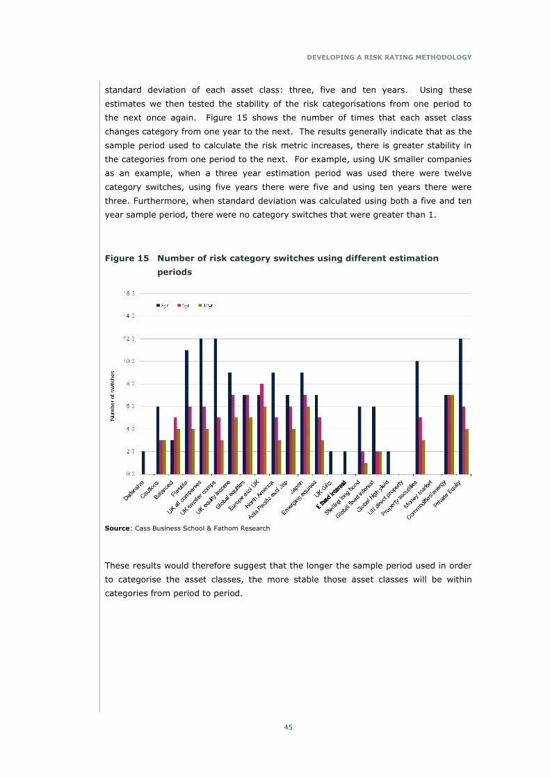
DEVELOPING A RISK RATING METHODOLOGY
45
standard deviation of each asset class: three, five and ten years. Using these
estimates we then tested the stability of the risk categorisations from one period to
the next once again. Figure 15 shows the number of times that each asset class
changes category from one year to the next. The results generally indicate that as the
sample period used to calculate the risk metric increases, there is greater stability in
the categories from one period to the next. For example, using UK smaller companies
as an example, when a three year estimation period was used there were twelve
category switches, using five years there were five and using ten years there were
three. Furthermore, when standard deviation was calculated using both a five and ten
year sample period, there were no category switches that were greater than 1.
Figure 15 Number of risk category switches using different estimation
periods
Source: Cass Business School & Fathom Research
These results would therefore suggest that the longer the sample period used in order
to categorise the asset classes, the more stable those asset classes will be within
categories from period to period.

JOINT ABI AND IMA RESEARCH PAPER, 2010
46
5.3 CESR‟s suggestions for risk bucketing
In its addendum to its consultation paper11 CESR outlined two proposals for setting the
volatility boundaries between risk categories, they refer to these as “volatility
intervals”. Each proposal sets out the minimum and maximum volatility boundaries
for each of six risk categories. These volatility boundaries had been set following
empirical research. The first set of intervals (Box 1, Option A, page 4) was designed
using a “stochastic optimisation process” to minimise the migration of funds from one
category to the next over 2008. The second approach produced a similar looking set
of volatility intervals (Box 2, Option B, page 5), but where the boundaries were drawn
to “avoid (the) excessive bunching” of funds into just one or two risk categories.
It is difficult to comment upon the actual volatility intervals presented in each box
without sight of the empirical study. Though it would seem fair to assume that option
A produced “excessive bunching” of funds into one or two categories. CESR asked for
views on the possible use of migration rules, and on using data with a different
frequency, but these issues are far less important than the two following issues:
the number of migrations of funds in each of the Lipper categories used for the
experiments and presented in the Appendix to the Addendum seem extremely
high, especially given the fact that this represents migrations over just one year,
albeit the particularly volatile year, 2008.
as we have already shown in this report, volatility rises and falls quite
dramatically from year to year. Given this how will these numbers be updated
from year to year? By contrast we have already demonstrated that relative risk
rankings between asset classes remain relatively stable from year to year over a
much longer period of time than used in the experiments by CESR.
11Addendum to CESR‟s consultation paper on the format and content of Key Information Document disclosures
for UCITS, August 2009.

DEVELOPING A RISK RATING METHODOLOGY
47
6.0 SURVEY OF PROFESSIONALS
6.1 Risk ranking and „professional sense‟
The results in Section 4 provide the basis for ordering broad investments according to
their risk characteristics. Standard deviation appears to provide the most stable
period to period ranking of the asset classes, but others seem almost as good, in
particular range, while downside deviation might be a better representation of risk
from an investor‟s perspective. However, one of the problems with assessing risk in
this way is that there may be some asset classes where the risks are not well
represented by a financial market index.
Within our data set there is one particular asset class that intuitively at least appears
to be ranked inappropriately. According to most of the risk measures we explored in
Section 3 the risk embodied by the UK direct property market, as represented by the
IPD total return index, is lower than that on a diversified portfolio of gilts as
represented by the FTA British government fixed all stocks index. But there are many
risks embodied by investments in commercial property that are not inherent in the
investment in a diversified portfolio of gilts, for example credit risk.
There are arguably two elements to the return on commercial property, rental income
and the gain that might accrue to the landlord from the sale of the property at some
point or the gain that might accrue as a consequence of being able to redevelop the
site at a profit when leases expire. To this extent then commercial property could be
characterised as being part corporate bond, where the rental income is analogous to
the coupon from a corporate bond, and part equity, since the capital value of the
property might generate a potentially large gain or loss for the commercial property
owner. Given this, it would seem inappropriate to rank the risk in this asset class
below a diversified investment in either corporate bonds or equity. Arguably, in the
risk spectrum, it should sit somewhere between these two asset classes, and certainly
above gilts.
The problem with the index as a representation of the risk inherent in commercial
property is that it is not based on the marked to market prices of commercial property.
Equity and bond indices are usually based upon securities that trade very frequently;
generally speaking property indices are based upon prices of assets that trade very
infrequently. This means that it may be unwise to compare the volatility of a
commercial property index with that of indices derived from more frequently traded
securities.
So asset class rankings based solely upon representative indices, may lead to some
intuitively unappealing conclusions. To shed further light on this issue we conducted a
survey of investment professionals to ascertain their views on the risk and return
characteristics of a range of asset classes.

JOINT ABI AND IMA RESEARCH PAPER, 2010
48
6.2 The survey
The survey set the respondents two tasks. They were presented with a randomised
range of investments, which also included two generic investment products. They
were then asked first to rank the asset classes on a scale of 1 to 6 according to their
expectation of both return and risk for each category, where category 1 represented
the asset classes that they expected to produce the lowest return and where 6
represented the asset classes that they expected to produce the highest return. They
were also asked to repeat this exercise using the same set of investment categories,
but where category 1 represented those asset classes with the lowest expected risk
and where 6 represented those asset classes in the highest expected risk category.
The survey questionnaire is shown in Appendix 3.
The survey was sent to investment professionals that comprised a combination of both
IMA and ABI members. The survey was completed by 73 respondents, representing
some of the largest fund management organisations and investment product providers
in the UK. The respondents worked in a variety of areas within these organisations but
all were primarily concerned with calculating or communicating information about their
investment products. Figure 16 presents the breakdown of respondents to the survey
by their function.
Figure 16 Role of respondent in organisation
Product design
Marketing
Management
Investment
Actuarial
Compliance
Other
Source: ABI, IMA, Cass Business School & Fathom Research

DEVELOPING A RISK RATING METHODOLOGY
49
6.3 Survey results
Table 6 presents the modal ranking of each of the investment categories used in the
survey. The order of the investments within each category does not imply anything
about relative risk. The results show that “cash” and “money market” investments
were seen as representing the least risky asset classes, while “emerging market
equities” and a set of alternative investment asset classes were ranked as representing
the set of most risky investments. We can also see from the table that “UK property”
is ranked above gilts and investment grade corporate debt and is placed in the same
category as for example “UK Balanced” which is a mixture of bond and equity
investment12. A UK equity investment is ranked in category 4, while category 5
includes higher risk equity investments, such as “smaller companies” and investment
in overseas developed economy equity markets that would involve an element of
currency risk.
The final column in Table 6 shows the percentage of respondents that assigned the
modal ranking to the asset class shown in column 2 of the table. There is the highest
degree of agreement with regards to cash as an asset class: 88% of the respondents
assigned “cash” a ranking of 1. However, agreement on the other investment
categories is generally much lower. For example only 29 of the respondents put
commercial property in category 3, 7 put it in category 2, while 5 put it in category 5
and 3 in category 6. The range of responses possibly indicates that some respondents
were putting more emphasis on current market conditions than others. At the time
the survey was conducted the UK‟s commercial property market was falling sharply. By
contrast global equity markets were beginning to recover from the sharp falls that
began in the summer of 2007.
12 The “Balanced” investment category represents a 60% investment in UK equities and 40% investment in gilts
(see Table 3.1).

JOINT ABI AND IMA RESEARCH PAPER, 2010
50
Table 6 Survey-based risk rankings
Note: The results in this table are based upon the survey questionnaire presented in Appendix 2. Source: ABI, IMA, Cass Business School & Fathom Research
So, what was the basis of the respondents‟ decisions? The questionnaire made it clear
that respondents were not expected to undertake any empirical work to help them
come to their views; instead they were asked to use their experience as investment
professionals – what we might also refer to as „professional sense‟.
Figure 18 presents the relationship between the rankings in Table 6 and those
obtained from using the risk metrics used in Section 4. The chart shows that the
correlation between professionals‟ judgement and downside deviation is the highest of
the set of correlations. However, there is really little to choose between this
correlation and that obtained using the ranks generated by standard deviation, range
and maximum drawdown. This result is probably just tentative confirmation that the
industry prefers to represent risk using volatility-based measures of risk. We should
also note once again that the two measures that stand out from this set are the

DEVELOPING A RISK RATING METHODOLOGY
51
Sharpe and Sortino ratios, where at best we can conclude that there is no correlation
between these risk measures and how investment professional think about risk, or at
worst that there is an inverse relationship between the risk measure and the views of
professionals.
Figure 17 Correlation between professional ratings and risk ratings based on
risk measures
-20%
0%
20%
40%
60%
80%
100%
Stdev Range Max Draw Sharpe Beta VaR(95) Down SD Sortino
Co
rrela
tio
n (
su
rvey
an
d h
isto
ric r
isk
)
Source: ABI, IMA, Cass Business School & Fathom Research
Table 7 An intuitive categorisation
Bucket Component
1 Cash
2 Government
3 Investment grade debt
4 High yield debt
5 Equity
6 Equity (high risk)
Source: Cass Business School & Fathom Research
As well as being fairly consistent with the data, intentionally or otherwise the
investment professionals may also be applying a risk model that is consistent with the
capital structure of a firm. For example, we know that in the event of firm failure that
equity holders are likely to lose everything, subordinated debt holders may also lose
everything, while holders of senior debt stand to lose less and may receive a
considerable amount of their initial investment back if the company is investment
grade, but less the worse the rating of the company. Table 7 attempts to capture this

JOINT ABI AND IMA RESEARCH PAPER, 2010
52
structure in six categories. Each category is only meant to be broadly representative of
the amount of risk that an investor might expect from this generic risk category.
Although there are some asset classes based on the professionals‟ modal risk rankings
that do not fit neatly into the categorisation in Table 7, there is broad agreement
between the two.
6.4 Summary
As far as we are aware the survey conducted for this report is the first of its kind.
Taking the modal results it has revealed that there is a relationship between these
„professional rankings‟ and more formal measures of risk. In addition, this professional
sense seems to be based upon the security of the claim that an investor can expect
from each investment. However, the results also reveal that there is still considerable
disagreement from one professional and/or investment firm and another. So much so
that if fund providers were left to categorise asset classes into a set of six risk
categories then the same asset class could easily be ranked as a “six” by one firm but
only as a “two” by another. The purpose of this study is to find a way to standardise
the approach to risk ranking so that investors are not presented by such contradictory
information.

DEVELOPING A RISK RATING METHODOLOGY
53
7.0 RECOMMENDATIONS
The results presented in Sections 4 show that any one of a set of risk measures could
be used to produce fairly reliable relative risk rankings based upon asset class data
from one period to the next. In quantitative terms standard deviation and range
performed best. Downside deviation performed well but not as well, but it could be
argued that this measure of risk captures those risks that retail investors really care
about, that is, downside risk.
In its two consultation papers13 on this issue CESR‟s recommendation was that
standard deviation should be the preferred, basic, simple risk measure. Although in
neither paper did CESR justify this choice empirically, our results here show that
standard deviation is the most consistent of these simple risk measures. Given the
close relationship between standard and downside deviation (see Figure 5), this report
will not take issue with CESR‟s recommendation.
The risk bucketing exercises presented in Section 6 demonstrated how the risk
classification system would almost certainly be more stable from one year to the next
the longer the sample period used to calculate the risk. Given that our preferred
approach, as outlined in Section 1 and as investigated throughout, is to base the risk
methodology on asset classes, the report also recommends that a minimum of ten
years of monthly data be used as the basis for the risk calculation.
7.1 The role for a Risk Assessment Committee
The work in this report has also shown that it might be necessary to apply judgement
to the risk ranking of asset classes. It might also be necessary to specify where the
boundaries are drawn, perhaps using a framework along the lines presented in Table
7. Simply dividing the range of all relevant asset classes into categories with equal
numbers of asset classes may not be the best way to define the risk boundaries.
Furthermore, the boundaries will also need to be monitored over time. For example,
an asset class may experience a short period of either reduced or enhanced volatility
which might mean that it „strays‟ marginally into an adjacent risk category if a purely
quantitative approach is used for the categorisation. There may exist then valid
reasons for not re-categorising the asset class. Finally, but not exhaustively, what if a
new asset class emerges, for example like hedge funds in the late 1990s? Even an
asset class based approach to categorising hedge funds would not have worked in
1998 since representative index data did not exist at the time.
13 “Consultation paper on technical issues relating to KID disclosures for UCITS (March 2009)”, and “CESR‟s
technical advice at level 2 on the format and content of KID disclosures for UCITS (July 2009)”.

JOINT ABI AND IMA RESEARCH PAPER, 2010
54
The fundamental basis of the risk methodology should be quantitative, but for the list
of non-exhaustive reasons cited above, this report recommends that the process itself
is overseen by a committee of independent risk experts that would decide on these
and other related issues. However, we should stress that it is not the view of this
report that this committee would be involved with the risk rating of particular funds,
only the maintenance of the methodology and its implementation.
7.2 Single asset class funds
With regard to single, long-only asset class funds the risk categorisation should be
relatively straightforward. Each fund would be rated with reference to the volatility of
an index that represents this asset class and that of the fund. The risk rating would
represent the lowest possible risk rating for the fund, since the volatility of the index
would represent the risk inherent in a large, well diversified and passive investment in
this asset class. There should be relatively few issues relating to data availability for
funds with less than ten years of trading history. Using this approach, both existing
and newly launched funds could all be rated fairly easily.
7.3 Multi-asset class funds
The rating of multi-asset class, long only funds is slightly less straightforward, since
there are unlikely to exist an exact financial market index-based representative of
every multi-asset class fund available to investors. However, as long as these funds
are comprised of asset classes that are rated a relatively straightforward procedure
could be applied.
This report recommends that the assessment of these funds should be based upon the
set of asset classes that comprise it, where each asset class within the fund is given an
appropriate weight. Using this weighted average return on the asset classes (that is
the indices) the relevant risk metric could then be calculated.
The process should involve the following:
From the fund‟s mandate a financial market index representing each of the asset
classes that the fund is permitted to invest in should be identified; these indices
should already have a single asset class, risk rating. These financial market
indices should form the basis of the fund‟s risk profile.
The individual asset classes that comprise the multi-asset class fund should be
ordered from most to least risky, according to the risk metric that is applied to
each asset class.
The relevant financial market indices should then be combined in the following
way. The most risky asset class should be assigned a weight equal to the
maximum permitted weight of this asset class in the fund, as laid out in the
mandate. If the fund can be comprised of 100% of this asset class, then the
multi asset class fund would effectively be rated as a single asset class fund,

DEVELOPING A RISK RATING METHODOLOGY
55
where this asset class would be the most risky permitted within the mandate.
However, where it is not 100%, the next weight is assigned as the maximum
weight allowed on the next most risky permitted asset class, and so until the
weight sum to 100%. This may mean that some of the permitted asset classes
will receive a weight of zero. In this process the risk rating is based upon the
asset class composition of the portfolio, and not on the individual risk rankings of
the asset classes in the fund. For example, suppose an investment product is
comprised of 50% of an asset class with an individual risk rank of 1 and 50%
with an individual risk rank of 5; in this case the risk rank of the product would
not simply be calculated as a weighted average of these two ranks, that is, 3.
Using these fixed weights, and the representative financial market indices, the
monthly historic return on this mix of asset classes can be reconstructed for the
preceding ten years. This set of returns would then provide the basis for
calculating the risk of the fund.
JOINT ABI AND IMA RESEARCH PAPER, 2010
56
8.0 STRUCTURED PRODUCTS
The aim of this project is to identify a simple measure of risk that could be used as the
basis for risk rating a wide range of investments including “structured products”. The
discussions with fund managers revealed that most (not all) were fairly sceptical that a
single measure of risk could be extended to include structured products. Others
suggested that it would not be appropriate anyway to classify these investments
alongside more traditional, long-only investment vehicles.
This project has concluded that the risk rating approach should be applied at the asset
class level, rather than at the product level, given the range of products available in
the market place. However, given the importance of structured products in today‟s
investment landscape, here we explore some of the issues that must be considered if
the ratings methodology is to be extended to encompass them.
Perhaps the biggest issue is the fact that there are so many structured products.
However, having said this we can identify two broad categories of structured product:
those that are sold as „capital guaranteed‟ products, and those that are of the
„enhanced income‟ variety. We will attempt to deal with both types here.
As well as being asked to place broad asset classes into six risk categories, the
questionnaire examined in Section 6 also asked respondents to rank capital
guaranteed and enhanced income products (see Appendix 3). The modal result was
that capital guaranteed products should be ranked in category 2 along with gilts. The
modal result for enhanced income products suggested that they should be categorised
one category higher along with high yield bonds and fund types comprising a mixture
of bonds and equities. We should also bear in mind that while nearly 50% of the
respondents picked category 2 for capital guaranteed notes, only 37% of respondents
picked category 3 for the enhanced income notes and just over 30% of the
respondents these products into category 4 or above. The considerable disagreement
within the industry about the appropriate risk ranking of these products is almost
certainly a function of the very, very wide range of structured products.
We will now try to illustrate the issues by considering generic versions of capital
guaranteed notes and income enhanced notes.

DEVELOPING A RISK RATING METHODOLOGY
57
8.1 Capital guaranteed notes
A capital guaranteed note effectively comprises an investment in a zero coupon, bank
bond and the simultaneous purchase of a call option on another financial market
security, generally a broad equity index.
8.1.1 Zero coupon bonds
A zero coupon bond is, as the name suggest, a bond that does not pay a regular
coupon, but only its face or principle value at its maturity date. To achieve a return on
a zero coupon bond that matures in five year‟s time and which has a face value of
£100, the investor must purchase the bond for less than £100 today. For example, if
an investor buys a zero coupon bond that matures in five year‟s time with a face value
of £100 for £71.30, we can show that the annual percentage return that an investor
would earn over the five years would be 7%.
8.1.2 Call options
A call option is one of the basic types of option. It confers on the buyer the right to
buy (but not the obligation) an asset at some time in the future at a price that is fixed
once the option is purchased. The buyer of the option pays a non-returnable fee,
known as the option premium, to the seller of the option. The fixed price is known as
the exercise, or strike price of the option.
Suppose that an investor buys a call option on a financial asset, which gives them the
right to buy this asset for £100 in 3 month‟s time. The option writer charges a
premium of £10 in return for selling the call option, which is the non-refundable option
premium.

JOINT ABI AND IMA RESEARCH PAPER, 2010
58
Figure 18 Pay-off from call option
-15.0
-10.0
-5.0
0.0
5.0
10.0
15.0
20.0
25.0
70 75 80 85 90 95 100 105 110 115 120 125 130
Price of underlying asset
Pay o
ff, £s
Source: Cass Business School & Fathom Research
Figure 18 shows the pay-off profile for the holder of this call option. If at the maturity
date of the option the price of the asset is lower than the strike price of £100 then the
option holder will not exercise their option, since it would be cheaper to buy the asset
in the open market. In this instance the option will expire out of the money and the
investor will not recover the £10 premium paid.
If the stock price at the option‟s expiry date is £110, then the investor will exercise the
option by buying the stock from the option writer at the exercise price of £100; they
could then make a £10 profit by selling the stock on the open market for £110.
However, since the investor paid £10 for the option initially, this means that the call
option buyer would „break even‟. If the stock ends the period above £110 the investor
makes a cash profit.
There are two points in particular worth noting about the pay-off profile for a call
option. First, the investor has limited downside and virtually unlimited upside
potential, since the value of the ordinary shares could theoretically rise without limit.
These two securities – the zero coupon bond, and the call option – can be combined
into one structure to produce a capital guaranteed note, of the following, generic kind.
8.1.3 The structure of capital guaranteed notes
Suppose an investor wishes to invest £100 in a typical capital guaranteed note.
£70.30 of this £100 might be used to buy a zero coupon that „promises‟ to pay the
investor £100 in five year‟s time, effectively generating a 7% annual return. The
remaining £29.70 of the investor‟s investment might then be used to buy a call option
on the FTSE-100 index that matures (expires) in five years‟ time. This option will
normally produce a profit for the investor if the market has risen sufficiently over the

DEVELOPING A RISK RATING METHODOLOGY
59
five year investment horizon. In this case, the investor receives £100 from the
investment in the zero coupon bond, plus any gain made from the option as a result of
the rise in the equity market. However, if the equity market does not rise sufficiently
over the investment horizon, or indeed if it falls over this period, then the call option
will expire worthless. In this event the investor simply receives the £100 from the
investment in the zero coupon bond. The investor‟s original capital is therefore
„guaranteed‟ regardless of the performance of the underlying equity market.
However, although the capital is guaranteed, receiving £100 back from an original
investment of £100 after five years would almost certainly represent a loss. This is
because the money could have been invested in a credit-risk free government security
over this same period that would have generated a positive return on the investment
rather than one of zero.
Second, the guarantee is only as good as the credit quality of the company providing
it. In the event that the firm issuing the zero coupon bond fails, the investor may
experience a loss of some or even all of their capital.
Finally, it is important to understand that the guarantee itself usually only relates to
the maturity date of the note. If the investor wishes to get their money back during
the life of the note before it matures, the value they would receive would be based
upon the value of the zero coupon bond and option at the time they wish to surrender
the note minus the costs involved to the issuer of buying back the note. Depending
upon the values of these three elements then, the investor could experience a loss of
capital if they sell back the note to the issuer before it matured.
Using financial market data on the values of zero coupon AA-rated bank bonds and the
data necessary to price a call option on the S&P50014 index, a series of generic capital
guaranteed notes were constructed, each with a maturity of 5 years. At the beginning
of the investment horizon we assume that an investor makes an investment in the
capital guaranteed note. Enough of this initial capital is allocated to buy a zero coupon
bond that will pay back £100 for every £100 invested at the maturity date of the
contract. The remainder of the initial capital is used to buy an “at-the-money” call
option on the S&P500 equity index that will expire on the maturity date of the note at
the same time that the zero coupon bond matures. This means that the investor will
effectively receive 100% of the performance of the S&P500 over the life of the note.
But if the S&P500 ends the investment period lower than its level when the note was
purchased, the call option will be worthless, and the investor will only receive their
original investment of £100 back.
One of the features of such a product is that when the equity market has fallen well
below the level that prevailed when the note was issued it will have the risk
characteristics of a zero coupon bond. Conversely if the equity market has risen
14 This index was chosen because the data needed to reconstruct the value of the call option over time was
sufficient to recreate the values of these notes over a long time horizon.

JOINT ABI AND IMA RESEARCH PAPER, 2010
60
substantially since the note was issued it will have the risk characteristics of the
financial security underlying the asset.
Figure 19 shows the risk characteristics of two notes, one which was written in January
1999 and a note with identical characteristics written on January 2004. The graph
shows the exposure of each note over time to the underlying security in the option,
which in this case is the S&P500 index. The note issued in January 1999 begins life
with almost 100% exposure to the equity market; this is because the equity market
rose strongly for the first year and half after the note was issued. This in turn meant
that the call option had a very high value. However, once the equity market began to
fall, so did the value of the option and its correlation with the underlying equity
market. By the end of its life the note had almost no correlation with the equity
market, this is because the option was almost worthless. At this point the note was
effectively a simple investment in a zero coupon bond, and therefore had the risk
characteristics of this kind of bond. Over its life then, the risk characteristics of the
note went from being almost identical to a long investment in a passive US equity
fund, to being equivalent to an investment in a zero coupon AA-rated bank bond.
Figure 19 Exposure of five year capital guaranteed note to the S&P500 index
0.0%
20.0%
40.0%
60.0%
80.0%
100.0%
1999 2000 2001 2002 2003
Delt
a o
f note
Jan-99
Jan-04
Source: Cass Business School & Fathom Research
For most of its life the note issued in January 2004 has a significant exposure to the
US equity market, until global equity markets collapsed, the option becomes worthless
and the note reverts to the risk characteristics of the underlying zero coupon, bank
bond.
In effect, the „asset allocation‟ of this product can change dramatically. It can
effectively switch from being a 100% investment in the financial security underlying
the call option to being a 100% investment in a bond. Figure 20 presents the average
exposure to the S&P 500 index experienced by a series of five year capital guaranteed
notes issued at the beginning of each year from 1994 to 2004. The average exposures

DEVELOPING A RISK RATING METHODOLOGY
61
of each note to the underlying equity market is shown by the blue bars. This average
can be thought of as being the proportion of the volatility of the note that is identical
to the volatility of the equity index. The range of the exposure to the equity market
over the note‟s lifetime, that is the maximum minus the minimum exposure, is shown
by the green bars. This range shows the instability of the effective asset allocation of
such contracts, an instability that will naturally effect the risk characteristics of the
contract too.
Figure 20 Average exposure to the underlying index and range
0%
20%
40%
60%
80%
100%
1994 1995 1996 1997 1998 1999 2000 2001 2002 2003 2004
Issue date (January)
Exposu
re t
o t
he u
nderl
yin
g
Average Range
Source: Cass Business School & Fathom Research
Figure 21 shows the volatility of each note (calculated using standard deviation) over
its five year life. The chart also shows the volatility of the S&P500 index, that of the
underlying zero coupon bond and the volatility of an investment in a government (risk
free) security over the same period. The note is not as risky (on this measure) as an
investment in US equities. However, it is clearly more risky than an investment in a
high grade zero coupon bond, or in a credit risk free asset issued by the UK
government.
The difference in the volatility of the S&P500 and the note shown in Figure 21, is one
measure of the value of the guarantee to investors that is provided by the underlying
zero-coupon bond. But as stated above, even in the event that the original capital is
returned, an opportunity cost will almost certainly be incurred. Figure 22 illustrates
this cost. Each bar in Figure 22 shows the annualised return difference between each
note and an investment in a five year UK government bond at the start of the
investment period. A positive value means that the capital guaranteed product
outperformed the „risk free‟ investment. The chart shows however that on many
occasions the capital guarantee did not protect the investor from experiencing a real
investment loss. Investing in a five year government bond for five years would have
left the investor better off than buying the note between 1998 and 2001 and then

JOINT ABI AND IMA RESEARCH PAPER, 2010
62
again in 2004. Clearly these results are very product specific, but they do nonetheless
demonstrate the sort of risk inherent in them.
Figure 21 Volatility of the note, its components and a credit risk free
investment
0.0%
1.0%
2.0%
3.0%
4.0%
5.0%
6.0%
1994 1995 1996 1997 1998 1999 2000 2001 2002 2003 2004
Issue date (January)
Month
ly s
tandard
devia
tion
S&P500 Note Zero Risk free
Source: Cass Business School & Fathom Research
Figure 22 Annualised return difference between the note and an investment
in a credit-risk free instrument
-10.0
-5.0
0.0
5.0
10.0
15.0
20.0
25.0
30.0
1994 1995 1996 1997 1998 1999 2000 2001 2002 2003 2004
Annual excess retu
rn
Issue date (January)
Source: Cass Business School & Fathom Research

DEVELOPING A RISK RATING METHODOLOGY
63
8.1.4 Recommendation: Capital guaranteed notes
A generic capital guaranteed note is not risk free. It should always be placed in a
category above government debt of a similar maturity. The note‟s value will nearly
always experience more volatility than the embedded zero-coupon bond; furthermore
the volatility of this bond will rise as the credit quality of the underlying organisation
that has issued the bond declines. However, the note‟s volatility will nearly always be
lower than that of the financial instrument that forms the basis of the underlying call
option. Overall then, a capital guaranteed note should be given a risk rating that is
either equal to or greater than that that would be awarded to the asset class to which
the underlying zero coupon bond belongs, but it should be lower than the risk rating
that would be appropriate for the asset class that forms the basis of the call option.
But this approach will only be possible where the structure of the note is as simple as
the one used in this example.
8.2 Enhanced income notes
It is impossible to understate the range of enhanced income notes that are currently
marketed to investors, but it is possible to outline the basic principles and structure of
an enhanced income note. The products are designed, as the name suggests, to
provide investors with an income that is higher than they might be able to achieve by
investing in any fixed income security (bond) or from investing in a high interest bank
or building society account.
Suppose for the sake of example that an investor could buy a five year AA-rated bank
bond with a yield of 6%. This means that if they held this bond to its maturity date it
could be expected to generate a return of around 6.0% a year over this period. The
first stage of an enhanced income note might involve using an investor‟s money to
purchase this bond, but clearly if the seller of the note did nothing else then the return
that the investor could expect would still be around 6%. However, as well as buying
the coupon paying bond on behalf of the investor, the note seller will also sell put
options based upon another financial market security, often an equity index. The sale
of these put options provides the seller of the note with additional funds that can be
used to buy more of the bond. In other words, for every £100 that the investor puts
into the note their investment in the underlying bond is something greater than this.
By selling these puts and using the proceeds to buy greater quantities of the bond the
income from the product can be enhanced.
For example, suppose that for every £100 invested in a five year enhanced income
note, the note seller raises an additional £25 from the sale of puts on the FTSE-100
index, and then uses the full £125 to purchase a five year corporate bond that is
yielding 6% in the open market. Rather than receiving a yield of 6% the income yield
on the note would be 7.5%. The more put options sold and the higher their value, the
more the income can be enhanced for the note investor.

JOINT ABI AND IMA RESEARCH PAPER, 2010
64
To understand why it may not be appropriate to place enhanced income products in an
asset class risk continuum we need to consider the nature of the risk that selling a put
option involves. A put option gives the holder of the option the right to sell an asset at
a pre-specified price, at or before a pre-specified date and at a pre-specified price. It
can be thought of as the converse of the call option described above.
Figure 23 shows the „at expiry‟ pay-off profile for a basic put option. In this instance
the holder of the option has the right to sell the underlying asset to the writer of the
option at a price of £100, and for this right the put holder has paid a price or premium
of 10. The seller of the put option (in the context of an income enhanced note this is
the buyer of the note) therefore receives this £10 as their fee for providing the put
buyer with this option. If the underlying asset, which could be an equity index, is
trading at £120, for example, the put holder would not exercise their option: why sell
the asset at a price of £100 under the terms of the option if they can sell it in the open
market at a price of £120? However, once the value of the underlying asset falls
below £100, the put holder can exercise their option at a profit. For example, if the
underlying asset falls to £90 the put holder can buy the asset in the open market and
sell it to the put seller under the terms of the option and realise a profit of £10; the
put seller realises a loss of £10 at the same time. At this point then the put holder and
put seller both break even. However, as the asset continues to fall in value the put
holder‟s gains rise, as do the put seller‟s losses.
Figure 23 The generic pay-off for writing a put option
-25.0
-20.0
-15.0
-10.0
-5.0
0.0
5.0
10.0
15.0
70 75 80 85 90 95 100 105 110 115 120 125 130
Price of underlying asset
Pay o
ff, £s
Source: Cass Business School & Fathom Research
Effectively the put option protects the holder from downside losses, in much the same
way that car insurance protects car owners from the economic consequences of the
theft of their car. This is an important analogy: sellers of put options are effectively
selling insurance to other investors against future losses. If the loss does not arise

DEVELOPING A RISK RATING METHODOLOGY
65
then the put seller keeps the premium paid by the put buyer for the option, in the
same way that an insurance company keeps the premium we pay for our car
insurance. As Figure 23 shows, the upside from this financial transaction for the put
seller is the value of the premium, but the downside is almost unlimited.
When an investor buys an enhanced income product, they are effectively insuring
other investors against a loss. Furthermore the option element of an enhanced income
product is usually far more complicated than the example used here. Often it will
involve more than one option.
These investment products are extremely difficult to value. Because of the optionality
embedded in them and the complexity that they represent it is not possible to identify
a single unambiguous method for determining their future volatility. However, there
are complex techniques and methodologies that can be used to estimate a probability
of loss for these products.15 It is then possible to map (albeit imperfectly) this
measure of risk with more standard measures that can be used to identify the risk in
broad asset classes, as outlined in Section 4.
The main problem with this approach is that there could be as many different
estimates of this value as there are estimators. In other words the results are highly
dependent upon the assumptions used in the modelling technique. For an approach of
this kind to work, product providers would all have to use a standardised risk
modelling package, so that when investors look at the risk rating results of different
enhanced income products they know that they are comparing like with like.
8.2.1 Recommendation: Enhanced income products
An enhanced income note generally involves the buyer of the note selling insurance to
other investors, as such the buyer is part investor part insurer. There is a bewildering
array of enhanced income notes, some where the investor could lose all of their
capital, others where there may be a floor under potential losses. The only limit to
their variety is the imagination of product providers. So far they have proved
themselves to be very imaginative. It is very possible that a product of this kind will
produce the high income that it is designed to produce. This will be the case when the
insured event, for example a greater than 30% fall in a particular equity index, does
not trigger a payout from the note investor to other financial market participants. In
this case the volatility of the return received by the investor could be zero. But when
the event does happen the losses can be very large. There are techniques for
calculating the probability of such losses but in no way could they be described as
simple. As such the results of a risk ranking based upon them, even when a
standardised model has been used to calculate this probability, will be too complex to
explain to most investors.
15 Based on the calculation of the “net delta” of the individual elements of the note.

JOINT ABI AND IMA RESEARCH PAPER, 2010
66
Overall then, this report recommends that products of the enhanced income variety
should at a minimum, attract the highest risk ranking used in any categorisation, or
possibly be placed in a separate risk category of their own, but which shows clearly
that this risk ranking is higher than all other risk categories.
8.3 CESR‟s suggestions for calculating the risk on structured products
CESR wished to include these products16 in the same risk continuum as the more
straightforward, long only investment products. Their suggestion was that a 95% VaR
could be calculated for these products and that this VaR could then be transformed
into a measure of standard deviation as shown in expressions 2.8 and 2.9. It is
possible to do this, but this report has serious reservations about this approach.
CESR suggested that the volatility of the underlying financial market index could be
calculated over a five year historic period. The volatility of this index could then be
combined with the other elements of the product along with a “pricing model” to
simulate the probable performance of the product over the previous five years. From
this simulation it would be relatively easy to estimate a 95% VaR value for a one year
holding period, since the investment product could be surrendered before it matures.
Adapting this process a little would allow the product provider to estimate the volatility
of the product under the assumption that it is held until maturity and therefore to
calculate a second 95% VaR value corresponding to this alternative investment
horizon. CESR suggests that both VaR values could be presented to investors.
There are number of problems with this approach:
With regard to historic simulation, the economic conditions that give rise to the
launch of a structured product today, may not have existed in the past. The
launch of these products is often very dependent upon the complex relationship
between option premia, corporate bond spreads, and money market rates that
exist at the time of the launch. Historic simulation may often be „creating‟ a
product that would not have existed in the past! Furthermore, some of these
structured products have been and will be based upon newly launched financial
market indices, so that a historic replication would be quite literally impossible.
CESR used the phrase “pricing model” which if read quickly may seem innocuous
enough. However, under these proposals every product provider would be at
liberty to use their own pricing model. These could vary greatly between one
provider and another. The existence of possible multiple pricing models would
clearly make a like for like comparison of these products across different
providers difficult, if not impossible.
16Addendum to CESR‟s consultation paper on the format and content of Key Information Document disclosures
for UCITS, August 2009, The Committee of European Securities Regulators, CESR/09-716.

DEVELOPING A RISK RATING METHODOLOGY
67
One alternative to the use of a “pricing model” might be to calculate the modified VaR
for the structured product, as shown in expression 4.1. This formula represents a non-
discretionary version of VaR where simple rules could be specified with regard to the
calculation of its elements. However, to apply it providers would still need to recreate
the product, so that its performance could be assessed in the period prior to its actual
launch.
In summary, calculating the risk of these products is the easy part, standardising that
VaR and subsequent volatility calculation however, is the hard part. CESR‟s proposals
as far as they concern these products would therefore almost certainly violate one of
the main aims of its work, which is to standardise the risk rating of investment
products.
8.4 Summary
This report has argued that the industry should attempt to rate broad asset classes.
In the case of simple guaranteed income notes, it is possible to see a mapping
between the note and these asset classes. Such a mapping is less obvious in the case
of enhanced income notes. The recommendation with regard to these products then is
that an asset class based approach be developed to rate the former, but that the latter
should be categorised separately in recognition of their unique characteristic as being
part insurance, and that this rating should be the highest available in any agreed
scale.

JOINT ABI AND IMA RESEARCH PAPER, 2010
68
9.0 ABSOLUTE RETURN FUNDS
9.1 What is an absolute return fund?
Absolute return funds represent a relatively new investment category. The aim of
such funds are to produce a positive return for investors irrespective of market
conditions. Most of these funds will have a target return that will be related to
underlying cash rates. A typical target will be to achieve a return equal to LIBOR17
plus X% per annum. The managers of these funds attempt to do this by making use
of the sort of investment techniques that until recently have been the preserve of the
hedge fund industry. There are three basic techniques that are used:
They may use derivative products such as futures and options to protect the
value of their assets from adverse market movements, to profit when asset
prices fall, or to increase their exposure to the market in order to enhance
returns when asset prices rise.
They are also permitted to short securities. This effectively involves the
manager of the fund borrowing a security from another investor which they then
sell at the prevailing market price. To close this position the manager then has
to buy the security back at some point and pass it back to the security lender. If
the price of the security has declined in the meantime then the manager will
make a profit, since they sell at one price and buy back at a lower price. The
difference between these two prices will represent the profit for the absolute
return manager‟s fund.
Finally the fund manager can use leverage to enhance the return on their
investments. In this context leverage involves the manager borrowing to invest.
As an example of how leverage works, consider the following. An investor buys
an asset for £100 at the start of the year and sells it for £110 at the end of the
year. Their return from this investment (ignoring any transactions costs etc) is
therefore 10%. However, now suppose the investor buys the same asset at the
start of the year for £100, but borrows £50 at a rate of interest of 5% to fund
half of the purchase. At the end of the year the investor sells the asset for £110,
pays back the £50 that it borrowed plus the interest of £2.50 (5% x £50),
leaving £57.50 representing a profit of £7.50, which on an original investment of
£50 represents a return of 15%. So the investor has enhanced the return on the
transaction. In fact, the higher the borrowed amount (the leverage) and the
lower the interest rate on the borrowed funds, the higher will be the return
enhancement.
17 LIBOR is a key, benchmark cash rate, that is normally closely related to the Bank of England‟s policy rate.

DEVELOPING A RISK RATING METHODOLOGY
69
By using these and other related techniques, such as „pairs trading‟18, the fund
manager can increase the returns on their fund and reduce the risks relative to a
traditional, long only investment fund. Indeed, these funds are sold with the
marketing line that they aim to provide investors with “equity-like returns for cash-like
volatility”. This is clearly a particularly appealing investment aim.
However, as well as increasing the number of ways that the manager can add value, it
also increases the number of ways that the fund manager can subtract value from the
fund. For example, in the leverage example above, had the security fallen in value to
£90 at the end of the year rather than rising to £110, the leveraged investor would
have realised a loss of -25%, rather than one of -10%.
The aim of this project is to identify a way of risk rating asset classes, but as with
structured products, absolute return funds are not an asset class. They make use of
alternative fund management techniques to manage an underlying asset class or set of
asset classes. It is the abilities of each individual fund manager that will determine
whether the fund is able to deliver on the promise of “equity-like returns for cash-like
volatility”. Given that the vast majority of academic research19 in this area suggests
that fund managers do not “possess alpha”, that is the consistent ability to beat the
market, it would seem inappropriate to risk rate these funds as being as risky as cash.
Even if an absolute return fund manager can deliver on this risk/return promise in the
future, the vast majority of absolute return funds have only been launched with in the
last two to three years.
9.2 Recommendations
Most if not all absolute return funds focus on a particular asset class. For example, an
absolute return fund might focus on UK smaller companies, or European equities, or on
the sterling investment grade market. The basis of the risk rating should therefore be
the basic asset class on which the fund focuses. Where the fund focuses on more than
one asset class, then it should be risk rated using the multi-asset class risk ranking
rules laid out in Section 7 of this report.
However, the industry may wish to consider an enhancement to the process described
in Section 7 in the case of absolute return funds. The existence of leverage can
significantly increase the volatility of investment outcomes. Under the UCITS
Directive, absolute return funds can employ investment powers such that a fund‟s risk
exposure may be increased up to a maximum of 200% of the fund‟s value. This may
be used to enhance the performance of the fund. The appropriate volatility calculation
18 Pairs trading involves, for example, buying the shares of a company that the manager expects to rise in value
and selling short the shares of another company, usually from the same sector, that the manager expects
to fall in value. 19
See for example Nitzsche D, Cuthbertson, K., O'Sullivan, N. (2008), 'UK Mutual Fund Performance: Skill or
luck?', Journal of Empirical Finance, 15(4), p.613-634; or Nitzsche D, Cuthbertson, K. and Clare, A. (2009),
'An Empirical Investigation into the Performance of UK Pension Fund Managers', Cass Working Paper.

JOINT ABI AND IMA RESEARCH PAPER, 2010
70
for the asset classes used in the fund could therefore be adjusted to reflect the impact
of leverage.
For example suppose that an absolute return fund focuses solely on UK large cap
stocks. Then the risk rating of the fund would put it in the same asset-based risk
category as a passive investment in the FTSE-100 equity index. But Table 9.1 shows
the impact of varying amounts of leverage on an investment in UK equities on a range
of risk measures. The calculations assume that the manager maintains the leverage at
all times in UK equities for the full sample period and is able to borrow at prevailing
money market rates. For range, standard deviation and downside deviation the cells
in the table show the percentage increase in the risk metric compared with no
leverage. For maximum drawdown the cells show the increase in the loss compared
with the maximum loss in the case of no leverage.
Table 8 The impact of leverage on a passive investment in UK equities
Leverage
10% 20% 30% 40% 50%
Range 9.8% 19.9% 29.7% 39.6% 49.6%
St dev 9.9% 19.8% 29.9% 39.8% 49.7%
Downside Deviation 10.3% 24.1% 34.5% 44.8% 55.2%
Max drawdown -2.70% -5.30% -8.00% -10.60% -13.20%
Source: Cass Business School & Fathom Research
Clearly leverage increases the size of both positive and negative returns, and therefore
the overall risk of the investment. We recommend that the volatility of the asset
classes that are to be used within an absolute return fund should therefore be
calculated on a leveraged basis. If the results, for example, indicate that a leveraged
position in UK large cap equities is sufficient to make this investment as volatile as an
investment in unleveraged, higher risk rating categories, then the risk rating for the
fund should reflect this higher risk.
The leverage proportion used to calculate the leveraged asset class risk metrics should
be the target, average leverage of the fund: the higher this target the higher the risk
represented by each asset class within the fund. This target leverage would have to
be declared in the disclosure documentation. However, if regulatory and industry
bodies wish to be more conservative then rather than using the „target leverage‟ they
could use instead the maximum leverage allowed in the fund.
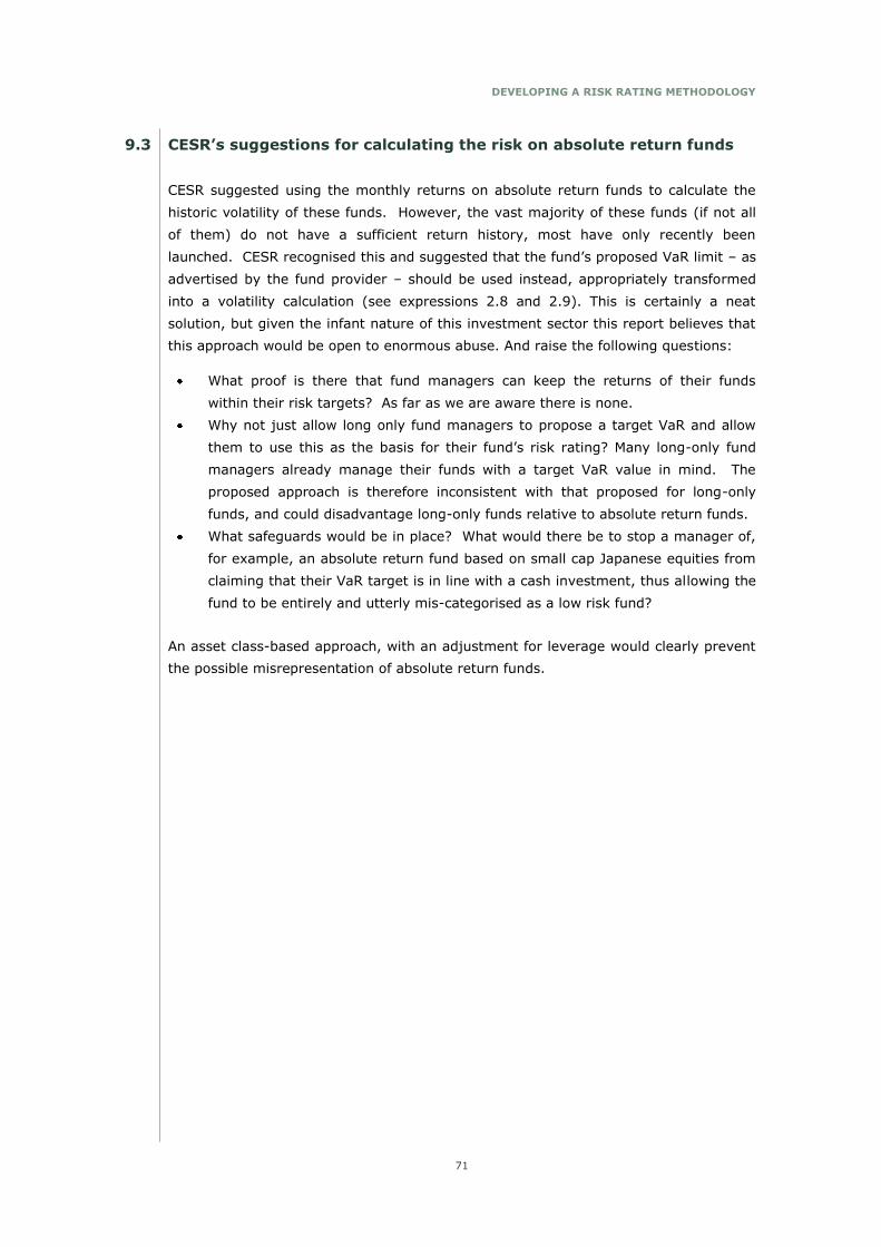
DEVELOPING A RISK RATING METHODOLOGY
71
9.3 CESR‟s suggestions for calculating the risk on absolute return funds
CESR suggested using the monthly returns on absolute return funds to calculate the
historic volatility of these funds. However, the vast majority of these funds (if not all
of them) do not have a sufficient return history, most have only recently been
launched. CESR recognised this and suggested that the fund‟s proposed VaR limit – as
advertised by the fund provider – should be used instead, appropriately transformed
into a volatility calculation (see expressions 2.8 and 2.9). This is certainly a neat
solution, but given the infant nature of this investment sector this report believes that
this approach would be open to enormous abuse. And raise the following questions:
What proof is there that fund managers can keep the returns of their funds
within their risk targets? As far as we are aware there is none.
Why not just allow long only fund managers to propose a target VaR and allow
them to use this as the basis for their fund‟s risk rating? Many long-only fund
managers already manage their funds with a target VaR value in mind. The
proposed approach is therefore inconsistent with that proposed for long-only
funds, and could disadvantage long-only funds relative to absolute return funds.
What safeguards would be in place? What would there be to stop a manager of,
for example, an absolute return fund based on small cap Japanese equities from
claiming that their VaR target is in line with a cash investment, thus allowing the
fund to be entirely and utterly mis-categorised as a low risk fund?
An asset class-based approach, with an adjustment for leverage would clearly prevent
the possible misrepresentation of absolute return funds.

JOINT ABI AND IMA RESEARCH PAPER, 2010
72
10.0 CONCLUSIONS
The empirical analysis presented in this report indicates that it is possible to identify a
relatively simple measure that can be used as the basis for measuring the risk inherent
in a wide range of investment funds, even to absolute return funds and also to certain
structured products, as argued in Sections 8 to 9. The basis for this calculation should
be the underlying asset classes from which the returns on these products are
ultimately derived, adjusted accordingly for any leverage.
This asset class-based approach has a number of advantages over the more fund-
based assessment process currently advocated by CESR. Most notably the fact that
asset class return data, for most asset classes are readily available in the form of
standardised financial market indices usually for significant periods of time.
Furthermore, many of these financial market indices are already used as benchmarks
for investment funds. Using these asset class proxies, combined with a
straightforward measure of risk it should be possible to risk rate new investment
funds, multi-asset class funds and even more complex investment products with data
that spans several business cycles, thereby adding to the likely stability of any risk
rating.
However, it seems almost entirely inevitable that there will be times when any purely
quantitative risk measure will produce what we might refer to as an „intuitive
anomaly‟. This might be because the available indices are an imperfect substitute for
actual investment in the asset class that it represents or due to market-related events
in a particular year. Furthermore, the boundaries of the risk buckets will need to be
drawn and monitored. With regard to drawing these boundaries there is no obvious or
simple quantitative approach to this issue.
Fund management groups and other investment product providers often create a risk
assessment committee to decide upon how their investment funds are categorised into
the risk buckets that they use in their own disclosure documents. This report proposes
that there is a similar role for a group of risk experts to oversee the risk rating process
at a national and/or EU-wide basis. This committee would be needed to:
make decisions about an appropriate set of asset classes and associated financial
market index proxies to be risk rated;
agree on the risk metric and methodology;
monitor market developments to ensure that the quantitative process does not
produce rating anomalies; and
monitor the risk category boundaries,
as well as other issues.
It is important to note that this report does not foresee a role for this committee that
would involve rating individual funds or even adjudicating where disputes regarding
individual funds arise. Taken together the quantitative, risk rating methodology and
the independent Risk Assessment Committee would instead provide the building blocks
for a process that would be used to risk rate all UCITs investment products.

DEVELOPING A RISK RATING METHODOLOGY
73
A1 REFERENCES
Blake, C., and M. Morey (2000), „Morningstar ratings and mutual fund performance‟, The
Journal of Quantitative Analysis, pp.451-483.
Blume, M. (1998), „An anatomy of Morningstar ratings‟, Financial Analysts Journal, pp.19-
27.
CESR, (2009a) „Consultation paper on technical issues relating to Key Information
Document (KID) disclosures for UCITS‟, March 2009, The Committee of European
Securities Regulators, CESR/09-047.
CESR, (2009b) „CESR‟s technical advice at level 2 on the format and content of Key
Information Document disclosures for UCITS‟, July 2009, The Committee of European
Securities Regulators, CESR/09-552.
CESR, (2009c) „Addendum to CESR‟s consultation paper on the format and content of Key
Information Document disclosures for UCITS‟, August 2009, The Committee of European
Securities Regulators, CESR/09-716.
Driver, R, Chater, N, Cheung, B, Latham, M, Lewis, R, and Stott, H, (2010) „Helping
consumers understand investment risk: experimental research into the benefits of
standardising risk disclosure‟, ABI Research Papers, forthcoming.
Fama, E. and K. French (1992), „The cross-section of expected stock returns‟, Journal of
Finance, pp. 427-465.
Favre, L. and J. Galeano, (2002), „Mean-modified Value-at-Risk optimization with hedge
funds‟, Journal of Alternative Investments, Fall.
Markowitz, HM., (1952) „Portfolio selection‟, Journal of Finance, pp. 77-91.
Morey, M., (2000), „Mutual fund age and Morningstar ratings‟, Working paper, Dept. of
Finance, New York University.
Nitzsche D, Cuthbertson, K., O'Sullivan, N. (2008), 'UK Mutual Fund Performance: Skill or
luck?', Journal of Empirical Finance, 15(4), p.613-634.
Nitzsche D, Cuthbertson, K. and Clare, A. (2009), 'An Empirical Investigation into the
Performance of UK Pension Fund Managers', Cass Working Paper.
Sharpe, W. (1964), „Capital asset prices: A theory of market equilibrium under conditions
of risk‟, Journal of Finance, pp. 425-442.
Stevens, P. and A. Lancellotta, (1995), „Improving mutual fund risk disclosure,
Perspective‟, Investment Company Institute, November.
Tversky, A. and Kahneman, D., (1991), „Loss Aversion in Riskless Choice: A Reference-
Dependent Model‟, The Quarterly Journal of Economics, pp 1039-61.

JOINT ABI AND IMA RESEARCH PAPER, 2010
74
A2 EARLIER WORK ON FUND RATINGS
There are many risk measures available. All these measures appear in a variety of
combinations on the fund sheets prepared by fund managers for their current and
prospective investors and for fund intermediaries. They are also calculated by
independent organisations that provide both quantitative and qualitative assessments of
funds, usually via a website that is made available to fund intermediaries.
However, there has been relatively little specific work by academics to establish which
risk measure best describes the risk inherent in an investment fund. However, the
academic literature has devoted some time to investigating Morningstar‟s risk adjusted
ratings (RAR) to ascertain whether the methodology can be relied upon to distinguish
between “good” and “bad” funds, ostensibly from within a single peer group.
Morningstar‟s original investment fund risk rating methodology is the only one that has
been investigated by academic researchers. The methodology made use of monthly
return data on each fund, where the constraint was that there had to be at least 36
monthly observations on each fund. The rating itself was a combination of two other
„ratings‟, one based upon return and another based upon risk.
The three year return rating20 involved calculating the cumulative return on the fund over
the previous three years and then subtracting from this the cumulative return over the
same period on a three month t-bill. This excess return was then divided by the higher of
the average excess cumulative return on funds in the same class, or the cumulative
return on the three month T-bills. The calculation is shown below:
)R)/n,R(Rmax(
RRRating Return
n
1k
ffk
m,fmk,
k (A1.1)
where Rk,m is the cumulative return over m months on fund k, Rf,m is the cumulative
return on a three month t-bill over the same m months, and n is the number of funds in
the same investment class as fund k.
The rating of fund risk has changed. But some of the original academic work on the
rating is based upon the original risk rating methodology, so we will review it briefly here.
The risk of each fund was calculated by using only those monthly returns that were below
the return achieved in that month on a three month t-bill; returns above the t-bill return
were set equal to zero. Thus the Morningstar risk methodology only looks at the
downside component of investment returns. The differences between the returns on the
fund and the t-bill rate were not squared, their absolute values were simply summed.
The risk rating calculation was then calculated as shown below:
20 Ratings can be calculated for any sample period.

DEVELOPING A RISK RATING METHODOLOGY
75
m
,0)Rmin(R
Rating Risk
m
1k
fk
k (A1.2)
The Morningstar rating for fund k was then calculated as the difference between these
two individual risk ratings:
KKK Rating RiskRating ReturnRating rMonrnigsta (A1.3)
The higher the rating the better the fund‟s performance.
Though widely used by the industry this rating process has been the subject of some
criticism by academic researchers. Blume (1998) pointed out that the choice of universe
can have a significant impact on the stars awarded to the funds. This is because the
returns are measured relative to those returns from the same investment group, or asset
class. Removing some funds from the peer group for example automatically changes the
ratings of those funds left in the group. Blume also found that younger funds tended to
have a more volatile rating over time than older funds. Work by Morey (2000) also
confirmed this point.
Of more interest to us here, Blake and Morey (2000) investigated the predictive ability of
the Morningstar ratings from one period to the next. They came to three broad
conclusions. First, that a low-rated fund tends to perform poorly in subsequent periods.
Second, that a highly rated fund will not necessarily perform well in subsequent periods.
These results are consistent with the findings of many academic papers, which is that,
poor performance tends to persist, while good performance does not. Finally, Blake and
Morey (2000) find that the Morningstar ratings are only marginally better than other
potential indicators of future risk and return such as the fund‟s prior performance, its
Sharpe ratio, Jensen‟s alpha coefficient and the four factor model of Blake et al (1996).
Since this early work on the Morningstar ratings, Morningstar have changed their rating
methodology. The risk rating component of their Morning Star rating – the Morningstar
Risk Adjusted Return (MRAR) – is now calculated as follows:
1R1
R1
T
1MRAR
12/2T
1t
2
bt
KtK (A1.4)
where Rbt is the return on a three month t-bill over month t. The Morningstar rating is
now given as:
KKK MRARRating ReturnRating rMonrnigsta (A1.5)

JOINT ABI AND IMA RESEARCH PAPER, 2010
76
The formulation of MRAR is rooted in expected utility theory (which we will not repeat
here). However, as far as we are aware no academic research has been conducted on the
performance of this revised measure.
The investment fund data provider, Lipper, also rates funds that belong in similar
investment groupings. The Lipper Preservation (LP) performance measure is calculated
as follows:
T
1t
KtK )Rmin(0,T
1LP (A1.6)
where T is the number of monthly observations over the assessment period (that is, 36,
60 or 120), and RKt is the return in month t of fund K. Essentially the measure averages
all the fund returns that are not positive. The highest value for LP would therefore be
zero. With Lipper‟s measure, a rolling T-bill investment would achieve this score, but
then so would any fund that had a positive return for each month in the estimation
period.
The Lipper measure, like the original Morningstar measure, also focuses on downside risk
rather than upside risk. However, as with the current Morningstar methodology, there
are no academic papers to my knowledge that test the predictive qualities of this rating
methodology.

DEVELOPING A RISK RATING METHODOLOGY
77
A3 RISK MEASURES FOR FULL SAMPLE
Notes: Each risk metric is calculated for each asset class or investment category using the
full sample of data (1987 to 1998).
0.00%
1.00%
2.00%
3.00%
4.00%
5.00%
6.00%
7.00%
8.00%
Standard deviation
0.00%
10.00%
20.00%
30.00%
40.00%
50.00%
60.00%
70.00%
Range
-40.00%
-35.00%
-30.00%
-25.00%
-20.00%
-15.00%
-10.00%
-5.00%
0.00%
Maximum drawdown
-20.00%
-15.00%
-10.00%
-5.00%
0.00%
5.00%
10.00%
15.00%
20.00%
25.00%
30.00%
35.00%
Sharpe
-0.20
0.00
0.20
0.40
0.60
0.80
1.00
1.20
Beta
0.00%
0.50%
1.00%
1.50%
2.00%
2.50%
3.00%
3.50%
4.00%
4.50%
5.00%
Down SD
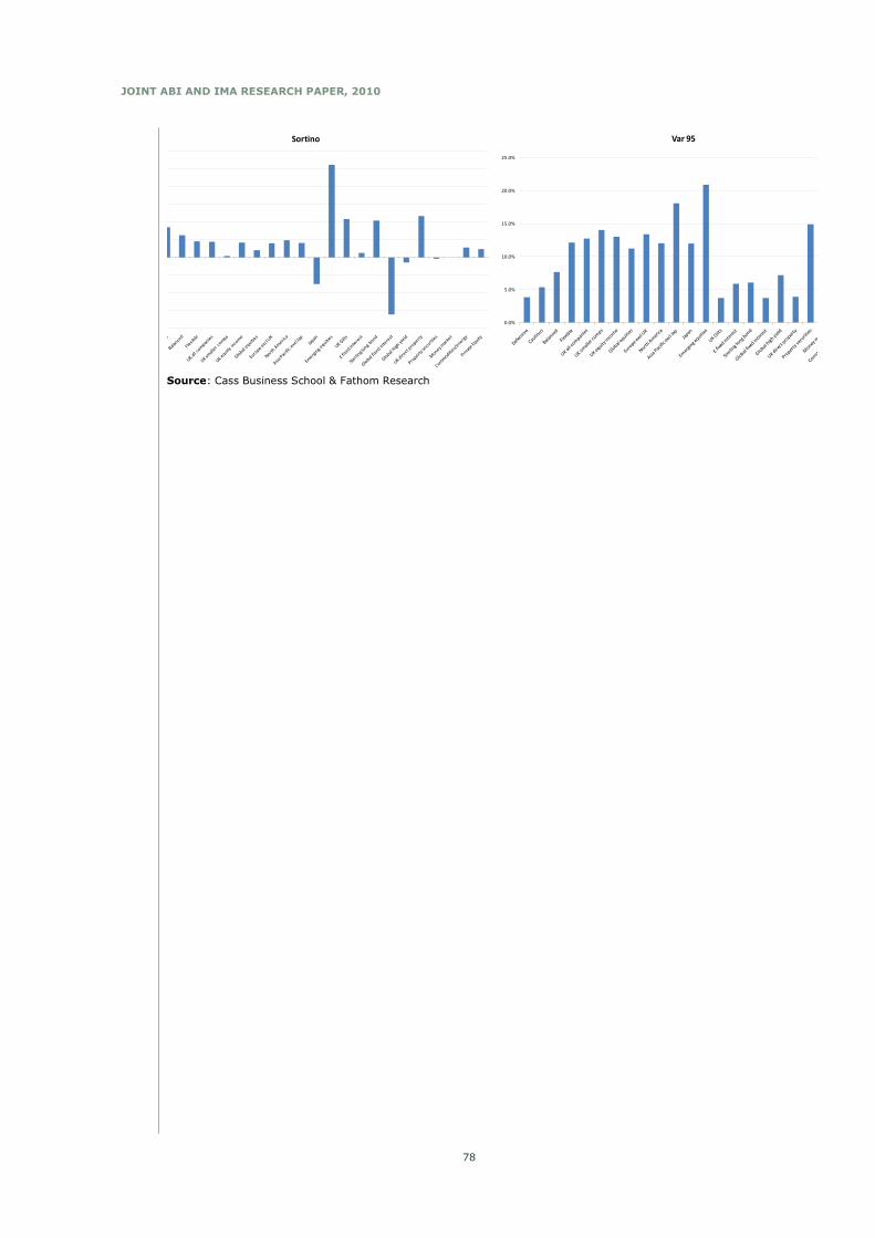
JOINT ABI AND IMA RESEARCH PAPER, 2010
78
-40.00%
-30.00%
-20.00%
-10.00%
0.00%
10.00%
20.00%
30.00%
40.00%
50.00%
60.00%
Sortino
0.0%
5.0%
10.0%
15.0%
20.0%
25.0%
Var 95
Source: Cass Business School & Fathom Research

DEVELOPING A RISK RATING METHODOLOGY
79
A4 THE RISK QUESTIONNAIRE
Risk assessment questionnaireIn column (2) r ank these asset classes/investment products according to their likely average
return in the future, where 1 is the lowest return category and 6 is the highest.
In column (3) r ank these asset classes/investment products according to their expected risk,
where 1 represents the least risky category and 6 the most.
(1) (2) (3)
Asset class/investment product Return category (1 to 6) Risk category (1 to 6)
Long gilt fund
Commodities
UK property
£ investment grade debt
UK Defensive
UK equity growth
Absolute return funds
Global property (excluding UK)
Cash (deposits)
UK Gilts
Emerging market debt
UK smaller companies
Global fixed interest (currency unhed ged)
£ Money market
UK Cautious
UK Balanced
North American equities
Emerging equities
Structured product (income product)
Private Equity
UK equity income
Asia Pacific excluding Japan
High yield
Japanese equities
UK equities
Hedge Fund (fund of funds)
European equities (ex UK)
UK large cap (FTSE -100)
Infrastructure
Structured product (capital guaranteed)
Global equities (ex UK)
Notes: Assume that all non -sterling based investments are currency unhedged . For the two
structured product categories - “Capital guaranteed” is some combination of zero coupon
bond and long call; while “income product” involves a coupon paying bond and short put
position.
Risk assessment questionnaireIn column (2) r ank these asset classes/investment products according to their likely average
return in the future, where 1 is the lowest return category and 6 is the highest.
In column (3) r ank these asset classes/investment products according to their expected risk,
where 1 represents the least risky category and 6 the most.
(1) (2) (3)
Asset class/investment product Return category (1 to 6) Risk category (1 to 6)
Long gilt fund
Commodities
UK property
£ investment grade debt
UK Defensive
UK equity growth
Absolute return funds
Global property (excluding UK)
Cash (deposits)
UK Gilts
Emerging market debt
UK smaller companies
Global fixed interest (currency unhed ged)
£ Money market
UK Cautious
UK Balanced
North American equities
Emerging equities
Structured product (income product)
Private Equity
UK equity income
Asia Pacific excluding Japan
High yield
Japanese equities
UK equities
UK smaller companies
Global fixed interest (currency unhed ged)
£ Money market
UK Cautious
UK Balanced
North American equities
Emerging equities
Structured product (income product)
Private Equity
UK equity income
Asia Pacific excluding Japan
High yield
Japanese equities
UK equities
Hedge Fund (fund of funds)
European equities (ex UK)
UK large cap (FTSE -100)
Infrastructure
Structured product (capital guaranteed)
Global equities (ex UK)
Notes: Assume that all non -sterling based investments are currency unhedged . For the two
structured product categories - “Capital guaranteed” is some combination of zero coupon
bond and long call; while “income product” involves a coupon paying bond and short put
position.
Source: ABI, IMA, Cass Business School & Fathom Research

Disclaimer: The analysis presented in this paper is based on research undertaken by the
authors and does not necessarily reflect the views of the Association of British Insurers,
the Investment Management Association or their member companies. The research was
carried out on behalf of the ABI and the IMA and is not intended to be relied on by a
wider audience. This paper is being published in order to contribute to public policy
debate and should be used only in that context. For that reason neither the author nor
the ABI or IMA shall have any liability for any loss or damage arising in connection with
the publication or use of this paper or the information in it. Neither the author nor the ABI
or IMA are authorised for the conduct of investment business (as defined in the Financial
Services and Markets Act 2000) and this paper is not intended as, and shall not
constitute, investment advice.
Copyright: Association of British Insurers and Investment Management Association,
2010. The information may only be used for private or internal use (provided that fair
attribution of copyright and authorship is made). This paper shall not be used for
commercial purposes (except for internal use, provided that the copyright and any other
proprietary notices are not removed). Reproduction in whole or in part, or use for any
commercial purpose (save as provided above) requires the prior written approval of the
Association of British Insurers and such consent may be withheld or made subject to
conditions.
ISBN 978 1-903193-51-6

For more information, contact:
Association of British Insurers
51 Gresham Street
London EC2V 7HQ
020 7600 3333
www.abi.org.uk
Investment Management Association
65 Kingsway
London WC2B 6TD
020 7831 0898
www.investment.org