Joint inference of identity by descent along multiple

chromosomes from population samples

Chaozhi Zheng†,(1), Mary K. Kuhner(2) and Elizabeth A. Thompson(1)

Department of Statistics Technical Report # 621

University of Washington

November, 2013

Running head: Joint inference of identity by descent

Key words: Latent identity by descent; shared genome segments; linkage disequilibrium;

hidden Markov model; Bayesian inference framework; reversible jump Markov chain Monte

Carlo.

(1) Department of Statistics, University of Washington, Seattle, WA, USA

(2) Department of Genome Sciences, University of Washington, Seattle, WA, USA

†: Current address: Biometris, Wagening University and Research Centre, Wageningen, The

Netherlands

1

Abstract

There has been much interest in detecting genomic identity by descent (IBD) segments from

modern dense genetic marker data, and in using them to identify human disease suscepti-

bility loci. Here we present a novel Bayesian framework using Markov chain Monte Carlo

(MCMC) realizations to jointly infer IBD states among multiple individuals not known to

be related, together with the allelic typing error rate and the IBD process parameters. The

data are phased single nucleotide polymorphisms (SNP) haplotypes. We model changes

in latent IBD state along homologous chromosomes by a continuous time Markov model

having the Ewens sampling formula as its stationary distribution. We show by simulation

that this model for the IBD process fits quite well with the coalescent predictions. Using

simulation data sets of 40 haplotypes over regions of 1 and 10 million base pairs (Mbp),

we show that the jointly estimated IBD states are very close to the true values, although

the presence of linkage disequilibrium decreases the accuracy. We also present comparisons

with the ibd haplo program which estimates IBD among sets of four haplotypes. Our new

IBD detection method focuses on the scale between genome-wide methods using simple IBD

models and complex coalescent-based methods which are limited to short genome segments.

At the scale of a few Mbp, our approach offers potentially more power for fine scale IBD

association mapping.

2

1 Introduction

Identity by descent (IBD) is a fundamental concept in genetics to describe the ancestral

relationships among current copies of homologous DNA. It was first introduced by Cotterman

(1940) and Malecot (1948) to generalize the coefficients of inbreeding and relatedness of

Wright (1921, 1922). Copies of DNA at a locus are IBD if they descend from the same

ancestral DNA. Thus IBD is by definition relative to some ancestral reference population.

The IBD state for a sample of homologous DNA copies can be specified as a partition into

disjoint sets; copies within a set share a common ancestor relative to the ancestral reference

population. To avoid confusion with alternate sets of chromosomes, alleles, or haplotypes,

we will refer to the members of the sample of haploid DNA copies under consideration as

gametes.

The concept of IBD has many uses in genetics, including detecting unknown familial

relationships (Stevens et al. 2011), family or population based genetic mapping (Albrechtsen

et al. 2009; Han and Abney 2011), genotype imputation and haplotype inference (Kong et al.

2008), measuring population structure (Weir and Cockerham 1984), and detecting natural

selection (Albrechtsen et al. 2010). There has therefore been much recent interest in inferring

IBD from genetic marker data, but the focus of these approaches has been pairs of gametes

or pairs of diploid individuals. Leutenegger et al. (2003) developed a method to estimate

inbreeding coefficients from individual genotypic data, and Browning (2008) used the same

model for pairs of population haplotypes. Purcell et al. (2007) and Albrechtsen et al. (2009)

summarize the latent IBD state at a locus as the number (0, 1, or 2) of gametes that are

IBD at the locus between two diploid individuals. Browning and Browning (2010, 2011)

further reduced the state space at a locus to none (0) or any (1) shared IBD between two

individuals. The primary goal of this paper is to extend the models and methods to inference

of IBD among an arbitrary number of gametes. This allows inference of joint patterns of IBD

among individuals and across a segment of genome for use in subsequent genetic analyses

(Browning and Thompson 2012; Glazner and Thompson 2012).

The complete historical relationship among current gametes can be described by the

3

genealogical tree of coalescent theory (Kingman 1982), in which ancestry is traced backward

in time from the present to the most recent common ancestor of the gametes. However,

for practical purposes, a reference population must be specified. In a pedigree-based study,

the gametes of the pedigree founders serves naturally as the reference population. In other

cases, there may be a well-defined founder population. However, in population samples

without external pedigree information, there is often no clear way to specify the ancestral

reference population. In this paper, we define IBD by specifying a reference population at t0

generations in the past. If mutations occurring subsequent to the t0 time point are ignored,

this specification is the same as the concept of equivalence class used by Kingman (1982) in

the formulation of the standard coalescent.

The choice of t0 will depend on the purpose of inferring IBD. Here we consider the

range of time depth t0 of tens to a hundred generations. This is “recent” IBD (Browning

2008; Browning and Browning 2010), intermediate between pedigree-based IBD among close

relatives and the ancient IBD that is a source of linkage disequilibrium (LD) in population

haplotypes. The time depth t0 is often specified indirectly by the probability η of IBD

between a pair of gametes. For a constant diploid population with effective size Ne, the

ancestral coalescence rate between two gametes is 1/(2Ne) and thus η = 1−exp [−t0/(2Ne)].

The pairwise probability η of IBD is approximately equal to the scaled time depth τ0 =

t0/(2Ne), for small time depth t0 (<102 generations) and large effective size Ne (>104 for

most recent human populations).

Since the IBD state at a site is the partition determined by a given time depth in the

genealogical tree, the process of changing IBD states along a chromosome is determined by

the process of changing genealogy due to historical recombination. In coalescent theory,

it has been shown that the sequence of coalescent trees along a chromosome can be well

approximated by a Markov process (McVean and Cardin 2005; Marjoram and Wall 2006).

Stam (1980) first introduced a Markov model for the IBD process between two gametes,

where the lengths of both IBD and non-IBD segments are exponentially distributed, and a

parameter λ measures the overall rate of change in IBD state. The two parameters η and

λ jointly determine the level of IBD at a site and the chromosomal extent of a segment of

4

shared ancestry (IBD).

Thompson (2008) developed a continuous time Markov model for four gametes with a

state space consisting of fifteen IBD states (the partitions of four gametes). Thompson

(2009) extended the model to any number n of gametes, but used it to infer IBD states

across a chromosome only for n = 2 and n = 4. In this model transitions in IBD state were

restricted to single gametes joining or leaving larger sets. Brown et al. (2012) relaxed the

restriction by allowing any move of one gamete between the subsets of an IBD partition and

implemented this model for sets of four gametes. Moltke et al. (2011) presented a model for

multiple gametes, but with much more restricted state transitions.

Model-based approaches to inference of latent IBD states from population single nu-

cleotide polymorphism (SNP) data generally use a hidden Markov model (HMM) approach.

This includes the original two-gamete model of Leutenegger et al. (2003) the generalizations

of Purcell et al. (2007) and Albrechtsen et al. (2009) to pairs of diploid individuals, and

the more general 15-state model implemented by Brown et al. (2012). These approaches

use exact HMM computational algorithms such as the forward-backward algorithm (Baum

et al. 1970; Baum 1972; Rabiner 1989).

In this paper, we extend the previous work of Brown et al. (2012) to jointly estimate

IBD along a chromosome among any number n of gametes using the same IBD process

model. However, exact HMM computations cannot be applied for larger numbers of gametes

because the state space increases extremely fast with n (Bell 1940). In the Methods section,

we develop a Bayesian inference framework and a reversible jump Markov chain Monte Carlo

(MCMC) method to estimate the latent IBD states along a chromosome, the IBD process

parameters, and the allelic typing error rate. Reversible jump MCMC is needed since the

number of IBD transition points can vary over MCMC realizations. We will call the new

method JointIBD.

Earlier methods computed IBD probabilities (Brown et al. 2012) or sampled IBD real-

izations (Moltke et al. 2011) only at locations of SNP markers. By sampling IBD transition

points, we achieve a more flexible MCMC process which realizes the IBD state at all points

on the chromosome. This means that a long stretch of bases without SNPs may contain

5

multiple IBD state transitions, allowing IBD state to change substantially between one SNP

and the next. Moltke et al. (2011) achieve a similar effect by allowing multi-step transitions

between marker locations.

JointIBD combines five extensions to previous approaches. (1) It can handle an arbitrary

number of gametes (we present results based on 40 gametes), as can the method of Moltke

et al. (2011), whereas other methods can handle only a small number. (2) It models the

full set of IBD partitions at a locus, and relaxes some restrictions on IBD state transitions.

(3) As do some earlier approaches, it explicitly models typing error, and as a byproduct

may be less sensitive to non-modeled recent mutations. (4) It allows transitions of IBD at

any point on the sequence, not only at SNP locations. (5) It provides Bayesian estimates

of parameters which can be related directly to the underlying processes of coalescence at a

locus, and recombination across the genome.

In the Simulations section, we show results using simulated data from Brown et al. (2012).

We compare JointIBD results for subsets of four gametes with results from exact compu-

tation using the ibd haplo program as implemented in the MORGAN v3.2 (2013) release

(http://www.stat.washington.edu/thompson/Genepi/MORGAN/Morgan.shtml). We con-

clude with a Discussion section.

2 Methods

2.1 The HMM Model

The data, y = {yij} consist of SNP haplotypes, with yij being the observed allele at SNP

site i (=1, .., m) of gamete j (= 1, . . . , n). Within the population, we assume that there

are only two alleles (denoted as allele 1 and allele 2) at each SNP site. Let ` be the length

of the chromosome in base pairs (bp), and let πi be the population frequency of allele 1 at

SNP site i. These allele frequencies are assumed to be known. In practice, they would be

estimated from a large population sample. We build a hidden Markov model for SNP data

y, where the latent variables are the IBD states across a genome segment.

6

At genome location x, the IBD state, Z(x), among gametes is represented as a partition

of the n gametes into IBD subsets, v, where each set is a collection of gametes that are IBD

at a location. Thus an IBD state at a site is a partition of the set of integers 1, 2, . . . , n. For

example n = 6, Z(x) = {{1, 2, 6}, {3, 5}, {4}} means that at a given location x gametes 1, 2

and 6 are IBD, gametes 3 and 5 are IBD, and gamete 4 is not IBD with any of the others.

The ordering of subsets and of the elements within each is irrelevant. Conventionally, here

we order the elements in each subset in increasing order, and order the subsets according to

the smallest member of each. The Ewens sampling formula (ESF, Ewens (1972)) provides a

single-parameter probability model for the n-gamete IBD partition at a site:

pn(z|θ) =Γ(θ)θ|z|

Γ(n+ θ)

∏

v∈zΓ(|v|), (1)

where θ > 0, |v| denotes the number of elements in set v, and Γ(v) denotes the Gamma

function. From equation (1), p2({{1, 2}} |θ ) = 1/(1 + θ). Thus, the parameter θ is inversely

related to the probability that two elements fall in the same subset, or, in our application,

that two gametes are IBD at this site. The pairwise IBD probability η is simply 1/(1 + θ).

We model the latent process of IBD transitions along chromosomes by a continuous-time

reversible Markov process whose stationary distribution is given by the ESF (1). We assume

that the distance to the next potential transition event along the chromosome is exponentially

distributed with mean 1/λ bp. Given current state z and a potential transition event, the

resulting IBD state w is sampled from the transition probability p(w|z) specified by the

modified Chinese restaurant process (MCRP, Brown et al. (2012)). Thompson (2009) and

Brown et al. (2012) model SNP-to-SNP transitions in IBD state, and so build in additional

flexibility by incorporating the possibility of IBD transitions independent of the current state,

where the new IBD state is sampled from the stationary ESF distribution (1). Since in our

model IBD transitions occur in a continuum, multiple state transitions can occur between

adjacent SNPs. There is therefore no need to include this additional model component.

We briefly describe the MRCP transition process as follows. First, insert a new gamete.

The gamete is inserted into any set of size k with probability k/(n+θ), or as a new singleton

with probability θ/(n+ θ). Next, randomly delete one of the n + 1 gametes. The newly

7

inserted gamete, if not deleted, takes the identity of the deleted one. Thus the MCRP allows

any one gamete to move from one IBD subset to another. It has been shown that the IBD

process along the chromosome is reversible with respect to ESF (Appendix A of Brown et al.

(2012)). Using the MCRP model, we formulate the transition probability for two consecutive

IBD states z and w along a chromosome. These transitions can result in the same IBD state

(z = w) or a different state (z 6= w).

The probability of a transition for which z = w is given by:

p(z | z, θ) =θ

(n+ θ)· a1 + 1

(n+ 1)+∑

v∈z

|v|(n+ θ)

· |v|+ 1

(n+ 1), (2)

where a1 denotes the number of singletons in z. Here the first term on the right hand side

refers to the case in which the new gamete is inserted as a singleton and one of the singletons

is then deleted, and the second term refers to the case in which the new gamete is inserted

into an existing set (denoted v) and one of the gametes in that set is then deleted. Since

some potential transitions do not produce state changes, the number of transitions predicted

by a given value of λ will generally be greater than the number of actual (i.e. state-changing)

transitions. Throughout this paper, whenever we measure the number of transitions or the

distance between transitions, we refer to actual transitions only. This is consistent with

usage in earlier methods (Leutenegger et al. 2003; Thompson 2009; Moltke et al. 2011).

In cases where the transition changes IBD state (z 6= w), suppose that the new gamete

is inserted into a set of size l1 and the deleted gamete is from a set of size l2. The transition

probability p(w | z, θ) is given by

p(w | z, θ) =

θ/(n+ θ) · (1 + I(l2 = 2))/(n+ 1)

l1/(n+ θ) · (1 + I(l1 = l2 = 1))/(n+ 1))

l1 = 0

l1 > 0, (3)

where I(S) = 1 if the statement S is true and 0 otherwise. This extra term arises when

one doubleton splits into two singletons (l1 = 0, l2 = 2) or two singletons merge into one

doubleton (l1 = 1, l2 = 1). The same state will result whichever of the two gametes is

deleted (for the former case) or inserted (for the latter case). For any two states z and w,

we define the IBD distance |z − w| to be the minimum number of IBD transitions necessary

to transfer one into the other according to the MCRP.

8

We model the emission probability of SNP data given the latent IBD states. We do

not model linkage disequilibrium in the ancestral reference haplotypes, so the SNP data

at each site i are conditionally independent given the latent IBD states. We assume that

the ancestral allelic states for each IBD subset are independent among subsets and across

sites, and are randomly sampled from a locus-specific ancestral allele frequency πi. Since we

consider common SNP variation and short scaled time depth τ0, we use separately estimated

current allele frequencies as proxies for πi.

Our typing error model assumes that each observed allele has a probability of ε of being

toggled to the alternative allele. Consider an IBD set of size l at site i. The probability

of the corresponding data vector consisting of, for example, k alleles of type 1 and (l − k)

alleles of type 2, is proportional to

πi(1− ε)kε(l−k) + (1− πi)(1− ε)(l−k)εk.

We assume that the scaled time depth τ0 defining the reference population is small enough

that mutations on the lineages from ancestral reference alleles to the current sample can be

ignored. Mutations which do occur will be interpreted as typing errors, potentially resulting

in an overestimate of ε.

For our Bayesian prior distributions on parameters, we assign priors of high variance

that suggest low levels of IBD among the n = 40 gametes. For the error probability ε, we

assign a uniform distribution on the range [0, 1]. For the IBD level parameter θ we use a

gamma distribution with shape αθ = 2 and scale βθ = 2n. This distribution has mean 160

and standard deviation ∼ 113, corresponding to values of η of order of magnitude 0.006,

but permitting much higher values where the data provide evidence of IBD. For λ we use a

gamma distribution with shape αλ = 2 and scale βλ = 10−4, giving a mean distance 5000

bp to the next potential transition point, but again allowing for much longer or shorter

segments.

For marker data with high levels of linkage disequilibrium (LD), our method tends to

overestimate IBD levels due to haplotype similarities in the reference founder population

(Purcell et al. 2007; Brown et al. 2012). This, in effect, increases the scaled time depth

τ0 of the ancestral reference population, and hence also the IBD level η. We therefore also

9

used a more informative prior distribution for θ by including a constraint, truncating the

gamma prior distribution, so that θ ≥ θc = n = 40. That is, the pairwise IBD probability

η is bounded above by 1/(1+θc). In addition, we restrict the total number of transitions to

be no greater than Kc = 2× 10−5`.

2.2 Parameter Estimation

We update Z(x) by reversible jump MCMC and the model parameters θ, λ, and ε by Gibbs

sampling. As the reversible jump MCMC procedure is the novel part of this process, we

describe it here: updates for other parameters are described in Supplemental Materials S4.

We define three proposal distributions for use in MCMC updates. These are briefly

described here; their formal definitions are in Supplemental Materials S3.

(1) The proposal distribution q(z|zA) or “one-side distribution” samples the IBD state of

the new z, starting from the left-side zA, using the MCRP. This could, for example, be used

to draw a new successor (z) to the most rightward interval on the chromosome (zA).

(2) The proposal distribution q(z|zA, zB) or “two-side distribution” samples a new z which

is an intermediate between the left side zA and the right side zB, which must be no more

than 2 steps apart; the new z must be no more than 1 step from each of zA and zB.

(3) The proposal distribution q(z|zA, zB, zC) or “propagation distribution” considers a

situation in which zA and zB are consecutive IBD states along the chromosome and are thus

no more than 1 step apart, and where zC is a state exactly 1 step from zA. If zB and zC

are no more than 1 step apart, the propagation stops, that is, z is set to zB. Otherwise, we

choose a new z which is no more than 1 step from both zB and zC , and is two steps from zA.

This proposal distribution is used when changes of an IBD state (modification, insertion,

or deletion) have to be propagated through a subsequent interval in order to avoid a violation

of the MCRP model. Proceeding rightward, new values for each of the IBD segments are

drawn from the propagation distribution where zB is the original state of the segment being

redrawn, zA is the state of its original leftward neighbor, and zC is the state of its current

leftward neighbor. This redrawing process stops as soon as a segment which is legal without

modification is reached, or at the end of the chromosome.

10

Updates of K, x, and z use six move types briefly described here (details and proposal

ratios are given in Supplemental Materials S4, as well as handling for special cases such as

the end of the chromosome).

(1) Update a transition location. A transition location is chosen at random and set to a

new location chosen uniformly between its flanking transitions.

(2) Update an IBD segment. A segment is chosen at random. A new state for this

segment is chosen from the two-side distribution, with its two neighbor IBD states being the

two sides.

(3) Update an IBD state with adjustments to downstream material. A segment is chosen

at random. A new state for this segment is chosen from the two-side distribution, with the

leftward neighbor and the current IBD state as zA and zB. Downstream IBD segments are

drawn from the propagation distribution.

(4) Insert a transition with adjustments to downstream material. A random IBD segment

is chosen and a new transition location is chosen uniformly within it. The new IBD state

associated with that transition is sampled from the one-side distribution based on its leftward

neighbor. The downstream IBD segments are drawn from the propagation distribution.

(5) Delete a transition with adjustments to downstream material. A random IBD segment

is deleted. The downstream IBD segments are drawn from the propagation distribution.

(6) Update segments of IBD by swapping their gamete labels. A pair of gametes is

chosen at random and partitioned into segments which are IBD and segments which are

not. Independently for each run of non-IBD material, we choose randomly whether or not

to swap the labels for that pair of gametes.

3 Results

3.1 Generation and analysis of simulated data

We test model performance using part of the population simulation of Brown et al. (2012).

In those data, a constant population of 3500 males and 3500 females was simulated over

t0 = 200 generations. In each generation, repeated 3500 times, a random male and a random

11

female were chosen to generate a son and a daughter. This mating system yields a mean

of 2 diploid offspring and a variance of 4, resulting in an effective population size of Ne =

7000 × 4/6 ≈ 4667 (Crow and Kimura 1970). The gamete segregating from a parent is

obtained by generating recombinants between the two homologous chromosomes of the parent

with rate 10−8 per bp. Each founder gamete is given a unique founder label; descendant

gametes are specified as a list of segments descending from the founder genomes with the

same label. Among a set of sampled gametes, homologous chromosome segments with the

same founder label are IBD.

The haplotypes of descendant individuals can be created by assigning founder haplotypes

to the labels. Briefly, Brown et al. (2012) generated founder haplotypes as follows. First a

BEAGLE haplotype cluster model (Browning and Browning 2007) was fit to a set of 1917

real haplotypes with high LD levels. These haplotypes also provided the assumed values of

the SNP allele frequencies πi. The program beaglesim (Glazner and Thompson 2012) was

then used to simulate new haplotypes from the BEAGLE model. In beaglesim, a parameter

γ controls generation of data sets at varying LD levels. In generating a haplotype from the

BEAGLE model, γ is the probability of random switching among haplotype clusters at each

SNP marker and thus LD is broken on average every 1/γ markers. In this paper we use only

the high-LD (γ =0.05) and no-LD (γ =1) data sets of Brown et al. (2012). We then impose

additional typing error on the data sets of Brown et al. (2012). After constructing the

current generation-200 haplotypes from the founder haplotypes and the descendant founder

genome segments, we simulate allelic typing errors using the same error model assumed by

our analysis. We apply error independently for each marker and each gamete with probability

ε=0.005.

Simulated data were analyzed with JointIBD as follows: For each data set, two inde-

pendent replicates were run. For each, 4 equally spaced temperatures were used, chosen

adaptively during burn-in. (The length of burn-in varied among the data sets.) After burn-

in, samples were taken every 20 iterations for a total of 20,000 iterations or 1000 samples.

The two replicates were pooled to give 2000 samples. Potential Scale Reduction Factors

(PSRFs, Gelman and Rubin (1992)) were computed between the two replicates to assess

12

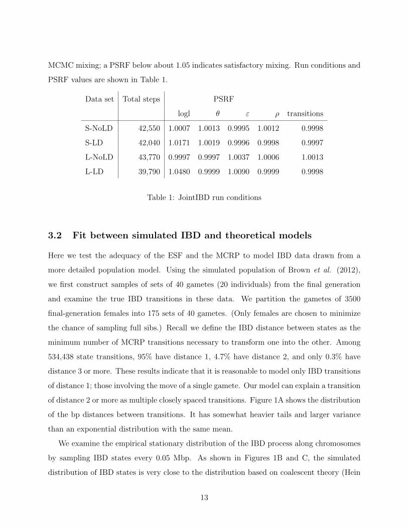
MCMC mixing; a PSRF below about 1.05 indicates satisfactory mixing. Run conditions and

PSRF values are shown in Table 1.

Data set Total steps PSRF

logl θ ε ρ transitions

S-NoLD 42,550 1.0007 1.0013 0.9995 1.0012 0.9998

S-LD 42,040 1.0171 1.0019 0.9996 0.9998 0.9997

L-NoLD 43,770 0.9997 0.9997 1.0037 1.0006 1.0013

L-LD 39,790 1.0480 0.9999 1.0090 0.9999 0.9998

Table 1: JointIBD run conditions

3.2 Fit between simulated IBD and theoretical models

Here we test the adequacy of the ESF and the MCRP to model IBD data drawn from a

more detailed population model. Using the simulated population of Brown et al. (2012),

we first construct samples of sets of 40 gametes (20 individuals) from the final generation

and examine the true IBD transitions in these data. We partition the gametes of 3500

final-generation females into 175 sets of 40 gametes. (Only females are chosen to minimize

the chance of sampling full sibs.) Recall we define the IBD distance between states as the

minimum number of MCRP transitions necessary to transform one into the other. Among

534,438 state transitions, 95% have distance 1, 4.7% have distance 2, and only 0.3% have

distance 3 or more. These results indicate that it is reasonable to model only IBD transitions

of distance 1; those involving the move of a single gamete. Our model can explain a transition

of distance 2 or more as multiple closely spaced transitions. Figure 1A shows the distribution

of the bp distances between transitions. It has somewhat heavier tails and larger variance

than an exponential distribution with the same mean.

We examine the empirical stationary distribution of the IBD process along chromosomes

by sampling IBD states every 0.05 Mbp. As shown in Figures 1B and C, the simulated

distribution of IBD states is very close to the distribution based on coalescent theory (Hein

13

et al. 2005) with scaled time depth τ0 = t0/(2Ne) ≈ 0.0214. The slight discrepancies may be

due to the use of only one realization of the underlying population pedigree or to differences

between the coalescent model and the simulation model used for IBD descent.

Figure 1B and D compare the simulation distribution with the ESF (Eq. 1). The value

of θ is set to 41 so that the mean number of IBD sets is the same as for the empirical

distribution. This is slightly smaller than the value calculated from the relation θ = (1 −η)/η ≈ (1 − τ0)/τ0 ≈ 46. The distribution of the number of IBD sets based on the ESF is

more dispersed than the simulated one (Figure 1B). Consistently, Figure 1D shows that the

more frequent IBD states are a little under-represented by the ESF while the less frequent

IBD states are a little over-represented. Overall, the ESF distribution fits the empirical

distribution reasonably well.

3.3 MCMC inference of IBD

To assess the performance of JointIBD we use the 40 haplotypes of the first 20 female indi-

viduals from the 200th generation of the simulated population of Brown et al. (2012). We

reset the location of the first marker as the origin. Bayesian estimation via MCMC simula-

tions is computationally intensive, and thus for each of the two data sets we analyze only the

initial 1Mbp (“short”) and 10Mbp (“long”) from each haplotype, corresponding to distances

used in fine scale gene mapping. We analyze four data sets: short and long haplotypes with

no LD (γ = 1, data sets S-NoLD and L-NoLD), and short and long haplotypes with strong

LD (γ = 0.05, data sets S-LD and L-LD). There are 85 markers in the 1Mbp data sets and

860 markers in the 10Mbp data sets. In the Figures results for no-LD data are shown on the

left throughout.

We first examine estimates from no-LD data for the parameters ε, θ, λ, and the average

density of IBD transitions (the number of transitions divided by the length of the chromo-

some). As shown in the left panels of Figure 2, the prior distributions (dashed lines) are

essentially non-informative. As expected, longer sequences give a tighter posterior distri-

bution. By chance, S-NoLD had a realized error rate of only 0.0035, while L-NoLD had a

realized error of 0.0053; as a result, the estimate of ε was low for the S data. The ESF pa-

14

rameter θ is estimated to be around 40 from both data sets (Figure 2C), which is consistent

with t0 = 200 generations (see section 3.1).

Since the “true” transition rate λ is unknown, we estimate it based on coalescent theory,

and then compare the result with its posterior distribution (Fig. 2E). The average number

of lineages (or IBD sets) at τ0 ≈ 0.0214 for n = 40 gametes is estimated to be around 28

(Hein et al. (2005); see also Figure 5A). The average total coalescent branch length L(τ0)

backward to τ0 can be obtained as L (τ0) =∑40

i=28 1/i = 0.387. Thus, from Ne = 4667 and

ρ = 10−8 per generation per bp we can roughly estimate λ = 2NeρL (τ0) ≈ 36 per Mbp. This

estimate falls in the range of the posterior distribution from S-NoLD, although it is slightly

larger than the estimate from L-NoLD.

The number of IBD state changes realized from S-NoLD (Figure 2G) is not significantly

smaller than the true empirical value of 18; the MCMC-based probability that this number of

actual transitions is more than 18 is 0.083. The number of actual IBD transitions estimated

from L-NoLD is around the true value of 169. Note that the transition rate λ suggests a

higher number of transitions than are actually realized, because some potential transitions

do not result in a changed IBD state.

Ancestral LD is due to shared population history beyond t0 generations in the past, and

is not accounted for in our model. Ancestral LD results in decreased θ and increased λ and

thus an increased number of IBD transitions (right panels of Figure 2). Figures 2D and H

show that, particularly for the large data set (L-LD), the estimated θ and the average density

of IBD transitions become very sharply distributed just above the truncation thresholds (see

section 2.1). As a consequence the posterior distribution of λ is essentially identical to its

prior (Figure 2E). Ancestral LD has effectively shifted the reference population backward and

increased the scaled time depth τ0. Our results confirm previous studies (Purcell et al. 2007;

Brown et al. 2012) showing that high LD regions are miscalled as shared IBD segments. The

mismatch between our model and the LD data also leads to an overestimate of the allelic

typing error rate (Figure 2B), since the miscalled IBD segments show strong haplotypic

similarity but not identity.

Figure 3 evaluates our estimation framework for the detection of IBD segments, begin-

15

ning with the transition locations. The cumulative distributions of IBD transition location

estimated from S-NoLD and L-NoLD are very close to the true distributions (Figure 3A

and C). Gray lines in Figure 3 panels B and D show the difference between the cumulative

distributions and the truth based on Figures 3A and C. Dark lines show the contrast with the

method’s performance in the presence of ancestral LD. Runs with LD deviate much further

from the truth, especially for S-LD.

To assess accuracy of state reconstruction, at each SNP marker location we evaluate the

inferred marginal IBD state by the probability that the distance between a random estimated

IBD state and the true IBD state is no greater than 2. As shown in Figure 4, IBD states

are not well estimated in the presence of LD in the founder genomes. This is explained by

the increased number of inferred IBD transitions (see Figure 2G and H) so that on average

fewer markers provide information about each IBD state. Estimation of IBD state is also

affected by the local density of SNP markers, as indicated by the poorer estimation of IBD

around the 8Mbp location in Figure 4C. There are only 31 SNP markers between 7.5 and 8.5

Mbp, far less than the global average of 86 markers per Mbp. As shown in the left panels

of Supplemental Figure S2, this region also shows high false positive probability and large

posterior uncertainties in the number of IBD subsets and pairwise IBD probability. Finally,

longer data sets do better than shorter ones in their area of overlap (Figure 4A and B),

presumably because of better parameter inference.

In addition, at each SNP marker location we evaluate the inferred IBD state by the number

of IBD subsets and the pairwise IBD probability. We define the false positive probability

at a location as the probability of a false claim of IBD between a random pair. Results

from the short data sets are shown in Figure 5, and from the long data sets in Supplemental

Figure S2. For the results estimated from S-NoLD (left panels of Figure 5), the true values

of the number of IBD sets and the pairwise IBD probability fall within their marker-specific

posterior central 95% intervals (Figure 5A and C), and the IBD states in the middle region

are well estimated as shown by the small posterior intervals (Figure 5A, C and E) and low

false positive probability (Figure 5E). In fact, a randomly sampled IBD state in the middle

region (0.35 to 0.7 Mbp) has a probability of around 0.91 being exactly the same as the true

16

state (data not shown).

In the presence of LD in the founder genomes (S-LD), the number of IBD sets at a

SNP marker in the middle region is underestimated (Figure 5B), consistent with our earlier

interpretation of the increased scaled time depth. This results in a larger pairwise IBD

probability and a higher false positive probability than in the absence of LD. However, even

in the presence of LD the rate of false claims of IBD remains below 1%.

3.4 Comparison with ibd haplo

Browning and Browning (2010, 2011) compared the performance of fastIBD to that of PLINK

(Purcell et al. 2007) and GERMLINE (Gusev et al. 2009), and Brown et al. (2012) compared

ibd haplo to fastIBD. Here we compare JointIBD to ibd haplo, using data based on those

in Brown et al. (2012). However, our results for ibd haplo performance are not directly

comparable to the previous results. First, the program has been substantially updated; we

used the version of the MORGAN v3.2 (2013) release. More significantly, Thompson (2009)

and Brown et al. (2012) incorporate the additional possibility of IBD transitions independent

of the current state. The ibd haplo program models SNP-to-SNP changes in IBD state, and

this additional flexibility may be important in area where SNPs are sparse. However, for

closer analogy with the JointIBD model, we do not here allow ibd haplo these additional

transitions. Finally, the data of Brown et al. (2012) did not include typing error, but an

error rate of 0.01 was used in the analysis, to accommodate aberrant IBD changes or (in real

data) mutations and other anomalies. In this paper, we added typing error at rate 0.005,

but used only this same lower value in the ibd haplo analyses.

For each of the two large data sets L-NoLD and L-LD, we ran ibd haplo for all 190

possible pairs out of 20 individuals, and obtained the most probable pairwise IBD state at

each marker location. In each run, we set ε = 0.005, the simulation value, and η = 0.025

so that θ = 39 close to the “true” value in terms of the number of IBD sets (Fig. 1B).

Following Brown et al. (2012), we used 0.05 per Mbp for the IBD change rate parameter

since the analysis of that paper has shown that keeping this parameter small provides more

robustness in the presence of LD. To compare with the results of Brown et al. (2012), we

17

first extracted the posterior distribution of pairwise IBD states from that of joint IBD states

among n = 20 individuals, and then found the most probable pairwise state for each pair of

individuals and at each marker location.

The results are shown in Figure 6. As shown in the left panels of Figure 6 for the

results estimated from data without LD, both methods perform very well and ibd haplo

performs slightly better than JointIBD. The number of pairs showing any IBD as estimated

by ibd haplo is almost identical to the true value, whereas JointIBD underestimates this

around the location of 7 Mbp (Figure 6A). ibd haplo shows fewer false IBD calls (Figure

6C) and fewer false no-IBD calls (Figure 6E). On the other hand, in the presence of LD

(right panels of Figure 6), JointIBD performs better than ibd haplo. The latter shows large

overestimation of the probability of any IBD (Figure 6B), which results in a large number

of false IBD calls (Figure 6D) at corresponding locations. Neither method does well at

detecting all the pairwise IBD (Figure 6F).

The differences in performance between ibd haplo and JointIBD are partly due to the

different specifications of the prior distributions. In the absence of LD in founder genomes,

the data are informative for the number of IBD transitions, and thus the results are not

sensitive to the ibd haplo assumption of a relatively low IBD change rate. The ibd haplo

program also fixed the parameter values of ε and θ, whereas JointIBD uses non-informative

prior distributions for these parameters. This may explain the slightly better performance

of ibd haplo.

In contrast, LD in founder genomes tends to be interpreted as IBD segments as such LD

is not modeled in these methods. Thus the number of IBD transitions is overestimated.

While ibd haplo puts a soft constraint on the number of IBD transitions by assigning a small

value to the IBD change-rate, JointIBD puts a hard upper bound on the number of IBD

transitions. Thus the false positive rate (calls of IBD given no IBD) is more effectively

controlled by JointIBD (Figure 6D).

18

4 Discussion

We have presented JointIBD, a Bayesian inference framework for the joint detection of IBD

segments among multiple gametes. We discuss three main assumptions in our model. First,

we assume that IBD processes along chromosomes are independent of allelic states. Thus,

the SNP loci are assumed to be selectively neutral and the effects of mutation negligible.

For the inference of IBD we use common SNP variation, not rare variants, and we aim to

infer IBD relative to a reference population at scaled time depth τ0 in the past. Processes

such as natural selection and demographic history are relevant only from τ0 to the present.

Our interest is in relatively recent IBD, where τ0 is of order 0.02. Therefore, in contrast

to detection of ancient IBD (large τ0), our method is largely immune to natural selection,

unless the selection is very strong.

The second main assumption is the modeling of IBD processes along chromosomes by

the modified Chinese restaurant process (MRCP) with the ESF as the stationary distri-

bution. In the ESF the gametes are exchangeable, and thus we implicitly assume there is

no geographical or social population structure among the small sample of individuals who

provide the gametes. To validate the ESF, we make comparisons with coalescent theory,

which assumes that the recent genealogical process of the population can be described by

a Wright-Fisher model with constant effective population size. We have verified that the

ESF is a good approximation of the probability distribution of IBD states at τ0 predicted

by coalescent theory, although the number of IBD subsets has slightly higher variance under

ESF (Figure 1B). The MRCP has an approximate biological basis. IBD transitions involv-

ing only one gamete correspond qualitatively to historical recombination events occurring on

terminal branches of coalescent trees along chromosomes in the sequential Markov coalescent

(McVean and Cardin 2005; Marjoram and Wall 2006). For small scaled time depth τ0, the

large majority of recombination events occur in the terminal branches.

Lastly, we assume that the ancestral allelic states for IBD sets are independent both

within loci and across loci. As we do not model LD in founder genomes, we have evaluated

its impact on detection of IBD segments. Our results have shown that LD is confounded with

19

the underlying IBD states, indicating the desirability of accommodating LD. Albrechtsen

et al. (2009) modeled the non-independence of marker data given hidden IBD states by

pairwise haplotype probabilities. Browning (2008) and Browning and Browning (2010) built

a joint hidden Markov model for haplotype frequencies and pairwise IBD states. Their

model for haplotype frequencies incorporating LD models localized haplotype clusters as

a variable-length Markov chain (Browning 2006). However, in order to estimate joint IBD

states among multiple gametes, we have necessarily simplified the data model. Joint inference

in the presence of LD remains an important direction for future work.

We have compared JointIBD to ibd haplo, using data from Brown et al. (2012). In the

absence of LD in founder genomes, both methods perform well, and comparably. In the

presence of LD in founder genomes, JointIBD controls the false positive calls of IBD more

effectively, but otherwise does not outperform ibd haplo in terms of inferring pairwise IBD.

It is not surprising that the pairwise summaries of IBD are similar under the two methods,

as both use almost the same model for the IBD process. However, although the output

of JointIBD can be reduced to a pairwise summary, there is no straightforward way to

obtain a joint inference from ibd haplo. The IBD states for all the 190 pairs of individuals

obtained separately from pairwise methods are not always consistent, and even at a single

locus probabilities of IBD states obtained from different pairs cannot be easily combined.

Combining pairwise inferences to form estimates IBD states among multiple individuals

across loci is a challenging open problem. It is joint information, such as is provided directly

by JointIBD, that helps to increase power in IBD-based mapping (Moltke et al. 2011).

The only comparable published method for detecting joint IBD states among multiple

individuals is that of Moltke et al. (2011). Both methods use MCMC and are thus compu-

tationally intensive, and neither accommodates LD. However, their model specifications are

very different. Moltke et al. (2011) use integer IBD indicators for a gamete at a locus, where

0 represents non-IBD with any other gamete (singletons) and gametes with the same positive

indicator are IBD. The authors modeled IBD processes across a chromosome by a reversible

birth and death process of zero indicators. Direct transitions between positive indicators are

not allowed, so they must be implemented by inserting intermediate zero indicators. Thus,

20

there are many more IBD transitions in their model than are required by the underlying

historical recombination events.

In contrast to the single ESF parameter, θ, the stationary distribution of IBD indicators

in Moltke et al. (2011) is determined by two parameters: the maximum positive indicator

and the probability of being a zero indicator. Whereas the parameter η = 1/(1 + θ) has

a natural interpretation as the pointwise probability of IBD between a pair of gametes, it

is not clear how the Moltke et al. (2011) parameters relate to the reference population or

to the descent from an ancestral origin allele to each IBD group. The maximum positive

indicator limits the number of non-singleton IBD groups. It was fixed to be 1, 2, or 3 in

various analyses of Moltke et al. (2011), but it is unclear how it should be set in practice.

JointIBD can only analyze haplotype data at this time. For genotype data, unknown

phase could potentially be integrated out using the methods described by Albrechtsen et al.

(2009) and Moltke et al. (2011). Missing data can be easily accommodated in our method,

for example, by assuming that data are missing independently of allelic type. Alternatively,

a program such as BEAGLE (Browning and Browning 2007) can be used to infer the most

probable phase and to impute missing allelic states, while incorporating additional informa-

tion contained in reference panels of data if these are available.

Software availability. JointIBD is freely available as Mathematica code from the web site

http://www.stat.washington.edu/thompson/pangaea.shtml.

Acknowledgments

We thank Serge Sverdlov and Jon Yamato for editing assistance. This research was supported

by National Institute of Health grants GM046255 (EAT and CZ) and GM099568 (EAT and

MKK).

21

References

Albrechtsen, A., T. S. Korneliussen, I. Moltke, et al., 2009 Relatedness mapping and tracts

of relatedness for genome-wide data in the presence of linkage disequilibrium. Genetic

Epidemiology 33: 266–274.

Albrechtsen, A., I. Moltke, and R. Nielsen, 2010 Natural selection and the distribution of

identity-by-descent in the human genome. Genetics 186: 295–308.

Baum, L. E., 1972 An inequality and associated maximization technique in statistical esti-

mation for probabilistic functions on Markov processes, pp. 1–8 in Inequalities-III; Pro-

ceedings of the Third Symposium on Inequalities. University of California Los Angeles,

1969, edited by O. Shisha. Academic Press, New York.

Baum, L. E., T. Petrie, G. Soules, et al., 1970 A maximization technique occurring in the

statistical analysis of probabilistic functions on Markov chains. Annals of Mathematical

Statistics 41: 164–171.

Bell, E. T., 1940 Generalized Stirling transforms of sequences. American Journal of Mathe-

matics 62: 717–724.

Brown, M. D., C. G. Glazner, C.Zheng, et al., 2012 Inferring coancestry in population

samples in the presence of linkage disequilibrium. Genetics 190: 1447–1460.

22

Browning, B. L., and S. R. Browning, 2011 A fast powerful method for detecting identity by

descent. American Journal of Human Genetics 88: 173–182.

Browning, S. R., 2006 Multilocus association mapping using variable-length Markov chains.

American Journal of Human Genetics 78: 903–913.

Browning, S. R., 2008 Estimation of pairwise identity by descent from dense genetic marker

data in a population sample of haplotypes. Genetics 178: 2123–2132.

Browning, S. R., and B. L. Browning, 2007 Rapid and accurate haplotype phasing and

missing-data inference for whole-genome association studies by use of localized haplotype

clustering. American Journal of Human Genetics 81: 1084–1097.

Browning, S. R., and B. L. Browning, 2010 High-resolution detection of identity by descent

in unrelated individuals. American Journal of Human Genetics 86: 526–539.

Browning, S. R., and E. A. Thompson, 2012 Detecting rare variant associations by identity

by descent mapping in case-control studies. Genetics 190: 1521–1531.

Cotterman, C. W., 1940 . A Calculus for Statistico-Genetics. Ph.d. thesis, Ohio State Univer-

sity. Published in “Genetics and Social Structure”, P.A. Ballonoff ed., Acaddemic Press,

New York, 1974.

Crow, J., and M. Kimura, 1970 An Introduction to Population Genetics Theory. Harper and

Row, New York.

23

Ewens, W. J., 1972 The sampling theory of selectively neutral alleles. Theoretical Population

Biology 3: 87–112.

Gelman, A., and D. B. Rubin, 1992 Inference from iterative simulation using multiple se-

quences. Statistical Science 7: 457–472.

Glazner, C. G., and E. A. Thompson, 2012 Improving pedigree-based linkage analysis by

estimating coancestry among families. Statistical Applications in Genetics and Molecular

Biology 11: Iss.2, Article 11.

Gusev, A., J. K. Lowe, M. Stoffel, et al., 2009 Whole population genome-wide mapping of

hidden relatedness. Genome Research 19: 318–326.

Han, L., and M. Abney, 2011 Identity by descent estimation with dense genome-wide geno-

type. Genetic Epidemiology 35: 557–567.

Hein, J., M. H. Schierup, and C. Wiuf, 2005 Gene genealogies, Variation and Evolution: A

Primer in Coalescent Theory. Oxford University Press, Oxford, UK.

Kingman, J. F. C., 1982 On the genealogy of large populations. Journal of Applied Proba-

bility 19A: 27–43.

Kong, A., G. Masson, M. L. Frigge, et al., 2008 Detection of sharing by descent, long-range

phasing and haplotype imputation. Nature Genetics 40: 1068–1075.

24

Leutenegger, A., B. Prum, E. Genin, et al., 2003 Estimation of the inbreeding coefficient

through use of genomic data. American Journal of Human Genetics 73: 516–523.

Malecot, G., 1948 Les mathematiques de l’heredite. Masson et Cie., Paris, France.

Marjoram, P., and J. D. Wall, 2006 Fast “coalescent” simulation. BMC Genetics 7: 16.

McVean, G., and N. Cardin, 2005 Approximating the coalescent with recombination. Philo-

sophical Transactions of the Royal Society of London (Series B) 360: 1387–1393.

Moltke, I., A. Albrechtsen, T. Hansen, et al., 2011 A method for detecting IBD regions

simultaneously in multiple individuals — with applications to disease genetics. Genome

Research 21: 1168–1180.

Purcell, S., B. Neale, K. Todd-Brown, et al., 2007 PLINK: a tool-set for whole-genome asso-

ciation and population-based linkage analyses. American Journal of Human Genetics 81:

559–575.

Rabiner, L. R., 1989 A tutorial on hidden Markov models and selected applications in speech

recognition. Proceedings of the IEEE 77: 257–286.

Stam, P., 1980 The distribution of the fraction of genome identical by descent in finite

random-mating populations. Genetical Research Cambridge 35: 131–155.

Stevens, E. L., G. Heckenberg, E. D. O. Roberson, et al., 2011 Inference of relationships

in population data using identity-by-descent and identity-by-state. PLOS Genetics 7:

25

e1002287.

Thompson, E. A., 2008 The IBD process along four chromosomes. Theoretical Population

Biology 73: 369–373.

Thompson, E. A., 2009 . Inferring coancestry of genome segments in populations. in Invited

Proceedings of the 57th Session of the International Statistical Institute, Durban, South

Africa, pp. IPM13: Paper 0325.pdf.

Weir, B. S., and C. C. Cockerham, 1984 Estimating F-Statistics for the analysis of population

structure. Evolution 38: 1358–1370.

Wright, S., 1921 Systems of mating. Genetics 6: 111–178.

Wright, S., 1922 Coefficients of inbreeding and relationship. American Naturalist 56: 330–

338.

26

HAL ææææææææææææææææææææææææææææææ

ææææææææææææææ

æææææ

ææææææææ

æææææææææææ

ææææææææææææ

æææææææææææ

æææææ

æææææææææ

æææ

ææææææ

ææææææææ

æ

æ

ææææææ

æææ

æ

æææææ

æ

æ

ææ

æ

æææ

æ

ææææ

æ

æ

ææææææ

ææ

ææ

ææ

ææ

æ

ææææ

æ

æææææ

ææ

æ

ææææ

æææææ

æ

æ

æææææææ

æ

æ

æ

ææææ

æ

æ

ææ

æ

æ

æ

æ

æ

æ

ææ

æ

æææ

æ

æ

æææ

æ

æ

æ

æ

æ

æ

æ

æ

æ

æææ

ææ

æ

ææææ

ææ

æææ

æ

æ

æææææææææææ æ æææ ææ æ æ

0.0 0.1 0.2 0.3 0.4 0.5 0.6 0.7

0.001

0.01

0.1

1

10

Mbp

Fre

qu

en

cy

HBL

20 25 30 35 40

0.00

0.05

0.10

0.15

Number of IBD subsets

Fre

qu

en

cy

HCL

0.000 0.005 0.010 0.015 0.020 0.025 0.030 0.0350.000

0.005

0.010

0.015

0.020

0.025

0.030

0.035

Coalescent probability

Em

pir

ica

lfr

eq

ue

ncy

HDL

0.000 0.005 0.010 0.015 0.020 0.025 0.030 0.0350.000

0.005

0.010

0.015

0.020

0.025

0.030

0.035

ESF probability

Em

pir

ica

lfr

eq

ue

ncy

Figure 1

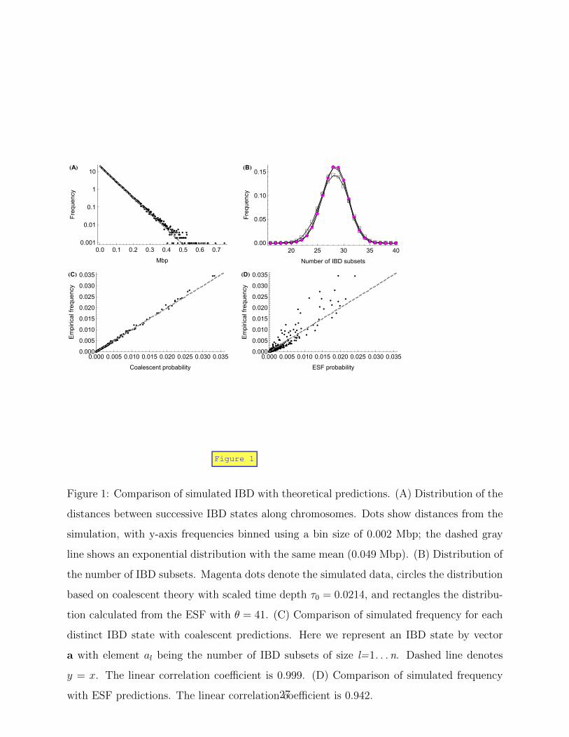
Figure 1: Comparison of simulated IBD with theoretical predictions. (A) Distribution of the

distances between successive IBD states along chromosomes. Dots show distances from the

simulation, with y-axis frequencies binned using a bin size of 0.002 Mbp; the dashed gray

line shows an exponential distribution with the same mean (0.049 Mbp). (B) Distribution of

the number of IBD subsets. Magenta dots denote the simulated data, circles the distribution

based on coalescent theory with scaled time depth τ0 = 0.0214, and rectangles the distribu-

tion calculated from the ESF with θ = 41. (C) Comparison of simulated frequency for each

distinct IBD state with coalescent predictions. Here we represent an IBD state by vector

a with element al being the number of IBD subsets of size l=1. . . n. Dashed line denotes

y = x. The linear correlation coefficient is 0.999. (D) Comparison of simulated frequency

with ESF predictions. The linear correlation coefficient is 0.942.27

HAL

0.000 0.002 0.004 0.006 0.008 0.0100

100

200

300

400

500

600

700

Allelic typing error rate ¶

Fre

qu

en

cy

HBL

0.000 0.002 0.004 0.006 0.008 0.0100

100

200

300

400

500

600

700

Allelic typing error rate ¶

Fre

qu

en

cy

HCL

0 20 40 60 800.00

0.05

0.10

0.15

0.20

ESF parameter Θ

Fre

qu

en

cy

HDL

0 20 40 60 800.00

0.05

0.10

0.15

0.20

ESF parameter Θ

Fre

qu

en

cy

HEL

0 10 20 30 40 500.00

0.05

0.10

0.15

0.20

IBD transition rate 106

Λ H1�MbpL

Fre

qu

en

cy

HFL

0 200 400 600 800 10000.000

0.001

0.002

0.003

0.004

IBD transition rate 106

Λ H1�MbpL

Fre

qu

en

cy

HGL

5 10 15 200.0

0.5

1.0

1.5

2.0

2.5

Average density of IBD transitions H1�MbpL

Fre

qu

en

cy

HHL

5 10 15 200.0

0.5

1.0

1.5

2.0

2.5

Average density of IBD transitions H1�MbpL

Fre

qu

en

cy

Figure 2

Figure 2: Posterior parameter distributions. Thin lines represent short data sets and thick

lines long data sets; left panels are no-LD results and right panels are LD results. Panels

show allelic typing error rate ε (A and B), ESF parameter θ (C and D), IBD transition rate

106λ (E and F), and average density of actual (state-changing) IBD transitions (G and H).

Cyan lines denote the marginal prior distributions, and the magenta dots in A and B denote

the true typing error rate (0.005). 28

HAL ÈÈ È ÈÈ ÈÈ È È È È È ÈÈ È È È È

0.0 0.2 0.4 0.6 0.8 1.00.0

0.2

0.4

0.6

0.8

1.0

xHMbpL

Cu

mu

lative

fre

qu

en

cy

HBL ÈÈ È ÈÈ ÈÈ È È È È È ÈÈ È È È ÈÈÈ È ÈÈ ÈÈ È È È È È ÈÈ È È È È

0.0 0.2 0.4 0.6 0.8 1.0

-0.2

-0.1

0.0

0.1

0.2

0.3

xHMbpL

Re

sid

ua

lfr

eq

ue

ncy

HCL ÈÈÈÈÈÈÈÈÈÈÈÈÈÈÈÈÈÈÈÈÈÈÈ ÈÈÈÈÈÈÈÈÈÈÈÈÈÈÈÈÈÈÈÈÈÈÈÈÈÈÈÈÈÈÈÈÈÈÈÈÈÈÈÈÈÈÈÈÈÈÈÈÈÈÈÈÈÈÈÈÈÈÈÈÈÈÈÈÈ ÈÈÈÈÈÈÈÈ ÈÈÈÈÈÈÈÈÈÈÈÈÈÈÈÈÈÈÈÈÈÈÈÈÈÈÈÈÈÈÈÈÈÈÈÈÈÈÈÈÈÈ ÈÈÈÈÈÈÈÈÈÈÈÈÈÈÈÈÈÈÈÈÈÈÈÈÈÈÈÈÈÈÈ

0 2 4 6 8 100.0

0.2

0.4

0.6

0.8

1.0

xHMbpL

Cu

mu

lative

fre

qu

en

cy

HDL ÈÈÈÈÈÈÈÈÈÈÈÈÈÈÈÈÈÈÈÈÈÈÈ ÈÈÈÈÈÈÈÈÈÈÈÈÈÈÈÈÈÈÈÈÈÈÈÈÈÈÈÈÈÈÈÈÈÈÈÈÈÈÈÈÈÈÈÈÈÈÈÈÈÈÈÈÈÈÈÈÈÈÈÈÈÈÈÈÈ ÈÈÈÈÈÈÈÈ ÈÈÈÈÈÈÈÈÈÈÈÈÈÈÈÈÈÈÈÈÈÈÈÈÈÈÈÈÈÈÈÈÈÈÈÈÈÈÈÈÈÈ ÈÈÈÈÈÈÈÈÈÈÈÈÈÈÈÈÈÈÈÈÈÈÈÈÈÈÈÈÈÈÈÈÈÈÈÈÈÈÈÈÈÈÈÈÈÈÈÈÈÈÈÈÈÈ ÈÈÈÈÈÈÈÈÈÈÈÈÈÈÈÈÈÈÈÈÈÈÈÈÈÈÈÈÈÈÈÈÈÈÈÈÈÈÈÈÈÈÈÈÈÈÈÈÈÈÈÈÈÈÈÈÈÈÈÈÈÈÈÈÈ ÈÈÈÈÈÈÈÈ ÈÈÈÈÈÈÈÈÈÈÈÈÈÈÈÈÈÈÈÈÈÈÈÈÈÈÈÈÈÈÈÈÈÈÈÈÈÈÈÈÈÈ ÈÈÈÈÈÈÈÈÈÈÈÈÈÈÈÈÈÈÈÈÈÈÈÈÈÈÈÈÈÈÈ

0 2 4 6 8 10

-0.2

-0.1

0.0

0.1

0.2

0.3

xHMbpL

Re

sid

ua

lfr

eq

ue

ncy

Figure 3

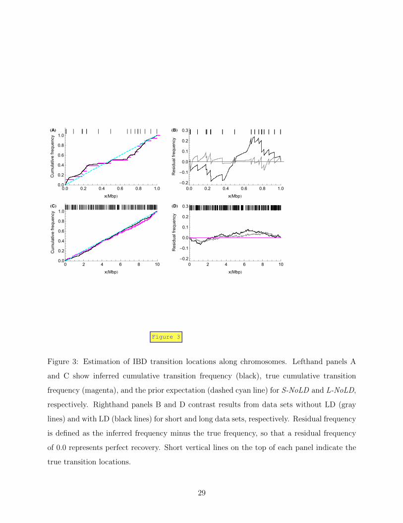
Figure 3: Estimation of IBD transition locations along chromosomes. Lefthand panels A

and C show inferred cumulative transition frequency (black), true cumulative transition

frequency (magenta), and the prior expectation (dashed cyan line) for S-NoLD and L-NoLD,

respectively. Righthand panels B and D contrast results from data sets without LD (gray

lines) and with LD (black lines) for short and long data sets, respectively. Residual frequency

is defined as the inferred frequency minus the true frequency, so that a residual frequency

of 0.0 represents perfect recovery. Short vertical lines on the top of each panel indicate the

true transition locations.

29

HAL

0.0 0.2 0.4 0.6 0.8 1.00.0

0.2

0.4

0.6

0.8

1.0

xHMbpL

Pro

ba

bility

HBL

0.0 0.2 0.4 0.6 0.8 1.00.0

0.2

0.4

0.6

0.8

1.0

xHMbpL

Pro

ba

bility

HCL

0 2 4 6 8 100.0

0.2

0.4

0.6

0.8

1.0

xHMbpL

Pro

ba

bility

HDL

0 2 4 6 8 100.0

0.2

0.4

0.6

0.8

1.0

xHMbpL

Pro

ba

bility

Figure 4

Figure 4: Detailed recovery of IBD states. Each panel shows the probability that the distance

between a random estimated IBD state and the true IBD state is no greater than 2 at each

SNP marker location. Throughout, heavy lines represent long datasets and narrow lines

represent short ones. Panel A contrasts S-NoLD and the first 1Mbp of L-NoLD ; panel B

contrasts S-LD and the first 1Mbp of L-LD. Panels C and D show results for the full length

of L-NoLD and L-LD, respectively.

30

HAL

0.0 0.2 0.4 0.6 0.8 1.018

20

22

24

26

28

30

xHMbpL

Nu

mb

er

of

IBD

su

bse

ts

HBL

0.0 0.2 0.4 0.6 0.8 1.018

20

22

24

26

28

30

xHMbpLN

um

be

ro

fIB

Dsu

bse

ts

HCL

0.0 0.2 0.4 0.6 0.8 1.00.00

0.01

0.02

0.03

0.04

0.05

xHMbpL

Pa

irw

ise

IBD

pro

ba

bility

HDL

0.0 0.2 0.4 0.6 0.8 1.00.00

0.01

0.02

0.03

0.04

0.05

xHMbpL

Pa

irw

ise

IBD

pro

ba

bility

HEL

0.0 0.2 0.4 0.6 0.8 1.00.000

0.005

0.010

0.015

0.020

0.025

0.030

xHMbpL

Fa

lse

po

sitiv

ep

rob

ab

ility

HFL

0.0 0.2 0.4 0.6 0.8 1.00.000

0.005

0.010

0.015

0.020

0.025

0.030

xHMbpL

Fa

lse

po

sitiv

ep

rob

ab

ility

Figure 5

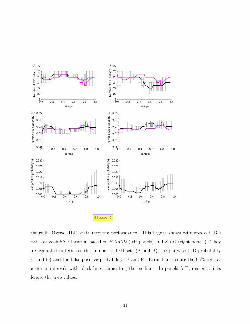
Figure 5: Overall IBD state recovery performance. This Figure shows estimates o f IBD

states at each SNP location based on S-NoLD (left panels) and S-LD (right panels). They

are evaluated in terms of the number of IBD sets (A and B), the pairwise IBD probability

(C and D) and the false positive probability (E and F). Error bars denote the 95% central

posterior intervals with black lines connecting the medians. In panels A-D, magenta lines

denote the true values.

31

HAL

0 2 4 6 8 100

50

100

150

xHMbpL

ðp

air

so

fa

ny

IBD

HBL

0 2 4 6 8 100

50

100

150

xHMbpL

ðp

air

so

fa

ny

IBD

HCL

0 2 4 6 8 100

20

40

60

80

100

120

xHMbpL

ðfa

lse

IBD

ca

lls

HDL

0 2 4 6 8 100

20

40

60

80

100

120

xHMbpL

ðfa

lse

IBD

ca

lls

HEL

0 2 4 6 8 100

5

10

15

20

25

30

xHMbpL

ðfa

lse

no

-IB

Dca

lls

HFL

0 2 4 6 8 100

5

10

15

20

25

30

xHMbpL

ðfa

lse

no

-IB

Dca

lls

Figure 6

Figure 6: JointIBD versus ibd haplo. Comparisons of JointIBD estimates (black lines) to

the pairwise estimates (cyan lines) obtained by ibd haplo from the data sets L-NoLD (left

panels) and L-LD (right panels). Magenta lines denote the true values. Panels A and B

show the number of pairs inferred to have any IBD. Panels C and D show the counts of false

IBD calls (false positives), and Panels E and F show the counts of false no-IBD calls (false

negatives). “No IBD” refers to the IBD state consisting of 4 singletons; all other IBD states

for two individuals are grouped as “any IBD”.

32

Supplemental Material

S1: The full posterior distribution

Following the notation in the main paper’s Methods section, the model parameters consist

of θ, ε, λ, and Z(x). We represent the transitions of IBD states Z(x) along chromosomes

by transition location xk and the resulting state zk = Z(xk) for k = 1, ..., K, where an IBD

transition occurs between nucleotide sites at xk − 1 and xk for k ≥ 2. For convenience we

set x1 = 1 and xK+1 = ` + 1, where ` is the length of the chromosome in base pairs (bp).

Let x = {xk}k=1..K+1 and z = {zk}k=1..K denote the vectors of transition points and IBD

partitions. Let s = {si}i=1..m and π = {πi}i=1..m, denote the vectors of SNP sites and their

minor allele frequencies. These allele frequencies π and SNP locations s are assumed to be

known. Finally, let yi = {yij}j=1..n denote the vector of observed alleles at SNP site i over

gametes j, and y = {yij}i=1..m,j=1..n the complete data over all gametes and sites. Note that

subscript i indexes the SNP sites, j the gametes, and k the IBD transition locations.

The full posterior distribution is given by

p(θ, ε, λ,K,x, z|y,π, s) ∝ p(y|π, s, K,x, z, ε) p(K,x, z|θ, λ) p(θ) p(λ) p(ε),

where each term is explained as follows. First, the SNPs are assumed to be independent

given the latent IBD state, so that the likelihood term is a product over SNP sites:

p(y|π, s, K,x, z, ε) =m∏

i=1

p(yi | Z(si), πi, θ, ε).

Additionally, since we assume independence of the allelic type of non-IBD DNA, each term

in the product over SNPs is again a product over the IBD subsets of gametes. Second, the

IBD process along the chromosome is modeled as a continuous time Markov process, with

the prior distribution given by

p(K,x, z|θ, λ) = p(z|K, θ) p(K,x|λ).

33

The probability of the vector z of IBD partitions is given by

p(z | K, θ) = p(z1 | θ)K−1∏

i=1

p(zi+1 | zi, θ),

where the distribution for the initial IBD state z1 is given by the ESF (main paper Equation

1), and the transition probability p(zi+1 | zi, θ) can be calculated from the modified Chinese

restaurant processes (MCRP) (main paper Equations 2 and 3).

Since λ� 1 and thus K � `, the geometrically distributed discrete inter-transition base-

pair counts are approximated by exponential distributions for the inter-transition distances.

That is, if K is not constrained,

p(K,x | λ) ∝ (1− λ)xK+1−xK−1K−1∏

i=1

((1− λ)xi+1−xi−1λ) ≈ λK−1e−λ`.

If K is bounded by Kc < ∞, the distribution of K will involve a normalization constant

that depends on λ. That is

p(K,x | λ) ∝ C(λ)λK−1e−λ`,

where C(λ) = Γ(Kc, λ`)/Γ(Kc), and the numerator is the incomplete Gamma function:

Γ(a, b) =∫∞bta−1e−tdt.

(Note C(λ) = 1 if Kc =∞.) Thus x is uniform on the space 1 = x1 < x2 < .... < xK+1 = `+1

and∫dx = `K−1/(K − 1)!. Then

p(K | λ) =

∫p(K,x | λ)dx =

C(λ)(λ`)K−1e−λ`/(K − 1)! if K ≤ Kc

0, if K > Kc

.

That is, the prior distribution for (K − 1) is a truncated Poisson distribution with mean λ`.

The prior distributions for θ and λ are Gamma distributions, where that for θ is bounded

below by θc. Thus if G[u | α, β] = (Γ(α)βα)−1uα−1e−u/β denotes the gamma probability

density on u > 0 with shape parameter α and scale parameter β, the prior distribution of θ

is

p(θ) ∝

G[θ | αθ, βθ] if θ ≥ θc

0 if θ < θc,

34

and the prior distribution of λ is

p (λ) = Γ[λ | αλ, βλ]

The prior distribution of ε is the uniform distribution in [0, 1]:

p(ε) =

1 if 0 ≤ ε ≤ 1

0 otherwise..

In general λ must be sampled via a Metropolis algorithm, but if Kc =∞ the full condi-

tional distribution for λ is the gamma distribution G(λ | (K + αλ − 1), (β−1λ + `)−1). In this

case λ can be integrated out to obtain the posterior distribution on the other parameters:

p(θ, ε,K,x, z | y,π, s) ∝ p(y | π, s, K,x, z, ε) p(z | K, θ) p(K,x) p(θ) p(ε), (S1)

where

p(K,x) =

∫p(K,x | λ) p(λ) dλ ∝ Γ(K + αλ − 1) (β−1λ + `)−(K+αλ−1).

S2: Possible transitions between two IBD states zA and zB

In this section we list all the transformations between two IBD states that differ by at most

two steps (|zA − zB| ≤ 2). In describing these transformations, we use lower case letters a,

b, c and d to denote gametes, and upper case X, Y , P and Q to denote IBD subsets. The

notation {a,X} will denote the subset {a}⋃X. Note that any specified gamete such as a is

not in any specified subset such as X. We denote the size of subset X by |X|, and group the

transformations by the pair of sizes (|zA|, |zB|) for the numbers of subsets in the two IBD

states that are involved in the transformation. Note that the IBD subsets shared between

zA and zB are irrelevant.

Case |zA − zB| = 0: If zA = zB no transformation is needed.

Case |zA − zB| = 1: Recall that one step of our process can move one gamete a from a

source subset S to a target set T . This move results from proposing the new gamete in set

T , and then deleting a from S, and the transformation is denoted (a : S → T ). In Table S1,

we give both the transformation from zA to zB and the transformation from zB to zA.

35

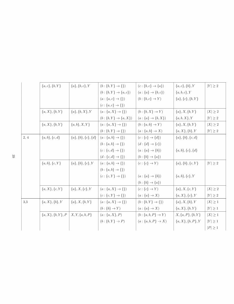
Case |zA − zB| = 2: In Table S2, we denote the intermediate state by zI , and give the

transformations from zA to zI and from zB to zI .

# subsets Subsets Subsets Transformation Transformation Condition

in zA, zB in zA in zB zA → zB zB → zA

1, 2 {a, b} {a}, {b} (a : {a, b} → {})(b : {a, b} → {})

(a : {a} → {b})(b : {b} → {a})

{a,X} {a}, X (a : {a,X} → {}) (a : {a} → X) |X| ≥ 2

2, 2 {a,X}, Y X, {a, Y } (a : {a,X} → Y ) (a : {a, Y } → X) |X| ≥ 1

|Y | ≥ 1

Table S1: List of transformations for |zA − zB| = 1.

36

# subsets Subsets Subsets Transformation Transformation Subsets Condition

in zA, zB in zA in zB zA → zI zB → zI in zI

1, 2 {a, b, c, d} {a, b}, {c, d} (a : {a, b, c, d} → {}) (b : {a, b} → {c, d}) {a}, {b, c, d}(b : {a, b, c, d} → {}) (a : {a, b} → {c, d}) {b}, {a, c, d}(c : {a, b, c, d} → {}) (d : {c, d} → {a, b}) {c}, {a, b, d}(d : {a, b, c, d} → {}) (c : {c, d} → {a, b}) {d}, {a, b, c}

{a, b,X} {a, b}, X (a : {a, b,X} → {}) (b : {a, b} → X) {a}, {b,X} |X| ≥ 3

(b : {a, b,X} → {}) (a : {a, b} → X) {b}.{a,X}1, 3 {a, b, c} {a}, {b}, {c} (a : {a, b, c} → {}) (b : {b} → {c})

(c : {c} → {b}){b, c}, {a}

(b : {a, b, c} → {}) (a : {a} → {c})(c : {c} → {a})

{a, c}, {b}

(c : {a, b, c} → {}) (a : {a} → {b})(b : {b} → {a})

{a, b}, {c}

{a, b,X} {a}, {b}, X (a : {a, b,X} → {}) (b : {b} → X) {b,X}, {a} |X| ≥ 2

(b : {a, b,X} → {}) (a : {a} → X) {a,X}, {b}2, 2 {a, b, c}, {d} {c}, {a, b, d} (a : {a, b, c} → {d}) (b : {a, b, d} → {c}) {b, c}, {a, d}

(b : {a, b, c} → {d}) (a : {a, b, d} → {c}) {a, c}, {b, d}(c : {a, b, c} → {d}) (d : {a, b, d} → {c}) {a, b}, {c, d}(c : {a, b, c} → {}) (d : {a, b, d} → {}) {a, b}, {c}, {d}(d : {d} → {a, b, c}) (c : {c} → {a, b, d}) {a, b, c, d}

{a, b,X}, Y X, {a, b, Y } (a : {a, b,X} → Y ) (b : {a, b, Y } → X) {b,X}, {a, Y } |X| ≥ 1

(b : {a, b,X} → Y ) (a : {a, b, Y } → X) {a,X}, {b, Y } |Y | ≥ 2

37

{a, b}, {c, d} {a, c}, {b, d} (a : {a, b} → {c, d}) (d : {b, d} → {a, c}) {b}, {a, c, d}(b : {a, b} → {c, d}) (c : {a, c} → {b, d}) {a}, {b, c, d}(c : {c, d} → {a, b}) (b : {b, d} → {a, c}) {d}, {a, b, c}(d : {c, d} → {a, b}) (a : {a, c} → {b, d}) {c}, {a, b, d}

{a,X}, {b} {b,X}, {a} (a : {a,X} → {b}) (b : {b,X} → {a}) X, {a, b} |X| ≥ 3

(b : {b} → {a,X}) (a : {a} → {b,X}) {a, b,X}(a : {a,X} → {}) (b : {b,X} → {}) X, {a}, {b}

{a,X}, {b, Y } {b,X}, {a, Y } (a : {a,X} → {b, Y }) (b : {b,X} → {a, Y }) X, {a, b, Y } |X| ≥ 1

|Y | ≥ 2

(b : {b, Y } → {a,X}) (a : {a, Y } → {b,X}) {a, b,X}, Y or |X| ≥ 2

|Y | ≥ 1

2, 3 {a, b, c}, {d} {a}, {c}, {b, d} (a : {a, b, c} → {}) (b : {b, d} → {c}) {b, c}, {a}, {d}(b : {a, b, c} → {d}) (a : {a} → {c})

(c : {c} → {a}){a, c}, {b, d}

(c : {a, b, c} → {}) (b : {b, d} → {a}) {a, b}, {c}, {d}{a, b,X}, Y X, {a}, {b, Y } (a : {a, b,X} → {}) (b : {b, Y } → X) {a}, {b,X}, Y |X| ≥ 2

(b : {a, b,X} → Y ) (a : {a} → X) {a,X}, {b, Y } |Y | ≥ 1

{a, c}, {b, d} {a}, {b, c}, {d} (a : {a, c} → {})(c : {a, c} → {})

(b : {b, c} → {d}) {a}, {c}, {b, d}

(b : {b, d} → {})(d : {b, d} → {})

(c : {b, c} → {a}) {b}, {d}, {a, c}

(b : {b, d} → {a, c}) (a : {a} → {b, c}) {a, b, c}, {d}(c : {a, c} → {b, d}) (d : {d} → {b, c}) {b, c, d}, {a}

38

{a, c}, {b, Y } {a}, {b, c}, Y (b : {b, Y } → {}) (c : {b, c} → {a}) {a, c}, {b}, Y |Y | ≥ 2

(b : {b, Y } → {a, c}) (a : {a} → {b, c}) {a, b, c}, Y(a : {a, c} → {})(c : {a, c} → {})

(b : {b, c} → Y ) {a}, {c}, {b, Y }

{a,X}, {b, Y } {a}, {b,X}, Y (a : {a,X} → {}) (b : {b,X} → Y ) {a}, X, {b, Y } |X| ≥ 2

(b : {b, Y } → {a,X}) (a : {a} → {b,X}) {a, b,X}, Y |Y | ≥ 2

{a,X}, {b, Y } {a, b}, X, Y } (a : {a,X} → {}) (b : {a, b} → Y ) {a}, X, {b, Y } |X| ≥ 2

(b : {b, Y } → {}) (a : {a, b} → X) {a,X}, {b}, Y |Y | ≥ 2

2, 4 {a, b}, {c, d} {a}, {b}, {c}, {d} (a : {a, b} → {})(b : {a, b} → {})

(c : {c} → {d})(d : {d} → {c})

{a}, {b}, {c, d}

(c : {c, d} → {})(d : {c, d} → {})

(a : {a} → {b})(b : {b} → {a})

{a, b}, {c}, {d}

{a, b}, {c, Y } {a}, {b}, {c}, Y (a : {a, b} → {})(b : {a, b} → {})

(c : {c} → Y ) {a}, {b}, {c, Y } |Y | ≥ 2

(c : {c, Y } → {}) (a : {a} → {b})(b : {b} → {a})

{a, b}, {c}, Y

{a,X}, {c, Y } {a}, X, {c}, Y (a : {a,X} → {}) (c : {c} → Y ) {a}, X, {c, Y } |X| ≥ 2

(c : {c, Y } → {}) (a : {a} → X) {a,X}, {c}, Y |Y | ≥ 2

3,3 {a,X}, {b}, Y {a}, X, {b, Y } (a : {a,X} → {}) (b : {b, Y } → {}) {a}, X, {b}, Y |X| ≥ 1

(b : {b} → Y ) (a : {a} → X) {a,X}, {b, Y } |Y | ≥ 1

{a,X}, {b, Y }, P X, Y, {a, b, P} (a : {a,X}, P ) (b : {a, b, P} → Y ) X, {a, P}, {b, Y } |X| ≥ 1

(b : {b, Y } → P ) (a : {a, b, P} → X) {a,X}, {b, P}, Y |Y | ≥ 1

|P | ≥ 1

39

{a,X}, {b, Y }, P {b,X}, Y, {a, P} (a : {a,X} → P ) (b : {b,X} → Y ) X, {b, Y }, {a, P} |X| ≥ 1

(b : {b, Y } → {a,X}) (a : {a, P} → {b,X}) {a, b,X}, Y, P |Y | ≥ 1

|P | ≥ 1

3, 4 {a,X}, Y, {b, c} X, {a, Y }, {b}, {c} (a : {a,X} → Y ) (b : {b} → {c})(c : {c} → {b})

X, {a, Y }, {b, c} |X| ≥ 1

|Y | ≥ 1

(b : {b, c} → {})(c : {b, c} → {})

(a : {a, Y } → X) {a,X}, Y, {b}, {c}

{a,X}, Y, {b, P} X, {a, Y }, {b}, P (a : {a,X} → Y ) (b : {b} → P ) X, {a, Y }, {b, P} |X| ≥ 1

|Y | ≥ 1

(b : {b, P} → {}) (a : {a, Y } → X) {a,X}, Y, {b}, P |P | ≥ 2

4,4 {a,X}, Y,{b, P}, Q

X, {a, Y },P, {b,Q}

(a : {a,X} → Y ) (b : {b,Q} → P ) X, {a, Y }, {b, P}, Q |X| ≥ 1

|Y | ≥ 1

(b : {b, P} → Q) (a : {a, Y } → X) {a,X}, Y, P, {b,Q} |P | ≥ 1

|Q| ≥ 1

Table S2: List of transformations for |zA − zB| = 2.

40

S3: The proposal distributions of an IBD state

We define three IBD proposal distributions used in the Metropolis type sampling from the

full posterior distribution (section S4).

1. One-side distribution. Let q(z|zA) be the proposal distribution where the IBD state z

is proposed from zA according to the MCRP.

2. Two-side distribution. Let q(z|zA, zB) be a proposal distribution for z as an interme-

diate state between zA and zB. Thus |zA − zB| ≤ 2, and the proposed z must satisfy

|z − zA| ≤ 1 and |z − zB| ≤ 1. We define q(z|zA, zB) for three cases:

• |zA − zB| = 0 (zA = zB). We sample z from q(z|zA).

• |zA − zB| = 1. We sample z = zA with probability 1/4, z = zB with probability

1/4, and otherwise generate the proposal by the following three steps:

– Insert a new gamete into a subset of zA of size j with probability j/(n+ θ),

or insert it as a new singleton with probability θ/(n+ θ).

– Delete the gamete that is deleted in a randomly chosen transformation from

zA to zB (see Table S1).

– Label the new gamete as the deleted one.

• |zA − zB| = 2. We list all the possible intermediate states, and randomly choose

one of them (Table S2).

3. Propagation distribution. Suppose that zA and zB are two consecutive IBD states along

the chromosome (|zA− zB| ≤ 1) and also that |zA− zC | = 1. Let q(z|zA, zB, zC) be the

proposal distribution of an IBD state z satisfying |z − zB| ≤ 1 and |z − zC | ≤ 1. Thus

there are four cases as shown in Figure S1.

• I: |zA − zB| = 0 and |zB − zC | = 1. Set z = zB.

• II: |zA − zB| = 1 and |zB − zC | = 0. Set z = zB.

• III: |zA − zB| = 1 and |zB − zC | = 1. Set z = zB.

41

Figure S1: The possible scenarios for state z under q(z|zA, zB, zC). The distance between

each pair of states is shown on the joining lines.

• IV: |zA − zB| = 1 and |zB − zC | = 2. Sample z uniformly from all the possible

IBD states satisfying the distance constraints (Table S2). If there is no such IBD

state, reject the proposal

Note that q(zB|zC , z, zB) is the reverse proposal distribution to q(z|zA, zB, zC).

Cases I and II are paired in this reversal, while cases III and IV remain unchanged.

S4 Sampling the posterior distribution via MCMC

We estimate the model parameters θ, λ, ε, K, x, and z by MCMC, using several versions of

the Metropolis algorithm. Our general notation for the target distribution of state variables

ω, is p(ω), and the proposal distribution for a new state given current state ωt is q(·|ωt). The

acceptance probability of proposed state ω∗ is

min

(1,p(ω∗)

p(ωt)/q(ω∗|ωt)q(ωt|ω∗)

). (S2)

If the proposal is accepted ωt+1 = ω∗, and otherwise ωt+1 = ωt. We refer to the ratio

p(ω∗)/p(ωt) in equation S2 as the target ratio, and the ratio q(ω∗|ωt)/q(ωt|ω∗) as the proposal

ratio. In the case of reversible jump MCMC, the acceptance probability also includes a

Jacobian factor (Green 1995).

42

The full conditional distributions of θ, ε and λ are given by

p(θ | ·) ∝ p(z | K, θ) p(θ)

p(ε | ·) ∝ p(y | π, s, K,x, z, ε) p(ε)

p(λ | ·) ∝ p(K,x | λ) p(λ) in general

and p(λ | ·) = Γ(λ|K + αλ − 1, 1/(β−1λ + `)

)if Kc =∞ (equation S1).

To sample θ, ε and λ from their full conditional distributions, we use random walk Metropolis

algorithms (Gelman et al. 1996) for each parameter separately (except in the case where λ

can be sampled directly). In this case the proposal ratio in equation S2 is equal to 1, and only

the target ratio is required. In each case the proposal distribution is a normal distribution

centered at the current value with the variance adjusted to give an acceptance ratio around

0.44 (Gelman et al. 2004).

Since the insertion or deletion of IBD change points involves a change in the dimension of

the parameter space, we update K, x, and z by reversible jump MCMC (Green 1995). We

use six move types in the sampler: (1) update a transition location, (2) update an IBD state,

(3) update an IBD state with downstream modification, (4) insert an IBD transition, (5)

delete an IBD transition, and (6) update segments of IBD states by swapping their gamete

labels. We denote by ϕi (i = 1...6) the sampling probability for move type i. In move types

(4-5), the parameter dimensions change by a transition location and an IBD state at the

location, and the Jacobian factor is 1.

In the following, we describe the proposals and give the proposal ratios for all the move

types (1-6), the target ratios for move types (4-5), and the full conditional distributions for

move types (1-3) and (6) from which the target ratio can be obtained.

1. Single update of a transition location. First randomly choose 2 ≤ k ≤ K, and then

sample a proposal value x∗k from a discrete uniform distribution in the range from

xk−1 + 1 to xk+1 − 1. The full conditional posterior distribution is

p(xk|·) ∝∏

{i|xk−1<si<xk+1}p(yi | Z(si), πi, θ, ε).

The proposal ratio is 1 as the proposal distribution is symmetric.

43

2. Single update of an IBD state. First randomly choose 1 ≤ k ≤ K. If there are no

IBD transitions (K = 1), a proposal state is sampled from q (z∗1 |z1). If the focal IBD

state is at an end of the chromosome (k = 1 or K ), a proposal state is sampled from

q (z∗1 |z2) for k = 1 and from q (z∗K |zK−1) for k = K. Otherwise, a proposal state z∗k is

sampled from q (z∗k|zk−1, zk+1). The full conditional posterior distribution is

p (zk|·) ∝∏

{i|xk≤si<xk+1}p(yi|Z(si), πi, θ, ε) p(zk+1|zk, θ) p(zk|zk−1, θ),

where p(zK+1|zK , θ) = p(z1|z0, θ) = 1 for the cases k = 1 or K.

The proposal ratio is

q(z∗1 |z1)/q(z1|z∗1) if K = 1, and otherwise q(z∗1 |z2)/q(z1|z2) if k = 1,

q(z∗K |zK−1)/q(zK |zK−1) if k = K, and otherwise q (z∗k|zk−1, zk+1) /q (zk|zk−1, zk+1) .

3. Single update of an IBD state with downstream modification. First randomly choose

k, 1 ≤ k ≤ K. If K = 1 or k = K, update using move type (2). If k = 1, sample

z∗1 from q(z∗1 |z1). Otherwise for k > 1, set z∗l = zl for l = 1 . . . k − 1, and sample z∗k

sampled from q(z∗k|zk−1, zk). If z∗k = zk we set l′ = k + 1. Otherwise we iteratively

sample z∗l from q(z∗l |zl−1, zl, z∗l−1) from l = k + 1 until there exists l′ ≥ k + 1 such that

z∗l′ = zl′ or l′ = K+ 1. If l′ < K, we set z∗l = zl for l = l′+ 1 . . . K. The full conditional

distribution is

p({Z(x)}xk≤x<xl′ |·) ∝∏

{i|xk≤si<xl′}p(yi|Z(si), πi, θ, ε)

l′−1∏

l=k−1p(zl+1|zl, θ),

where p(zK+1|zK , θ) is set to be 1 for l′ = K + 1. The proposal ratio is given by

q(z∗k|zk)q(zk|z∗k)

∏l′−1l=k q(z

∗l |zl−1, zl, z∗l−1)∏l′−1

l=k q(zl|, z∗l−1, z∗l , zl−1)

if k = 1, and otherwise (1 < k < K) by

q(z∗k|zk, zk−1)q(zk|z∗k, z∗k−1)

∏l′−1l=k q(z

∗l |zl−1, zl, z∗l−1)∏l′−1

l=k q(zl|, z∗l−1, z∗l , zl−1)

44

4. Insert one IBD transition. First randomly choose k, 1 ≤ k ≤ K. Then insert an

IBD transition location into x to give x∗ with x∗k+1, sampled from the discrete uniform

distribution in the range from xk + 1 to xk+1− 1. Set z∗l = zl for l = 1 . . . k, and insert

z∗k+1 sampled from q(z∗k+1|zk). If k = K we set l′ = K + 2, and if z∗k+1 = zk we set

l′ = k+ 2. Otherwise we iteratively sample z∗l from q(z∗l |zl−2, zl−1, z∗l−1) from l = k+ 2

until there exists l′ ≥ k + 2 such that z∗l′ = zl′−1 or l′ = K + 2. If l′ < K + 1, we set

z∗l = zl−1 for l = l′ + 1 . . . K + 1. The target ratio is

p(K + 1,x∗, z∗|·)p(K,x, z|·) =

∏{i|x∗k<si<x∗l′}

p(yi|Z∗(si), πi, θ, ε)∏{i|xk<si<xl′−1} p(yi|Z(si), πi, θ, ε)

∏l′−1l=k p(z

∗l+1|z∗l , θ)∏l′−2

l=k p(zl+1|zl, θ)p(K + 1,x∗)

p(K,x),

where the term p(K + 1,x∗)/p(K,x) is replaced by p(K + 1,x∗|λ)/p(K,x|λ) if λ is

sampled (equation S1), p(zK+1|zK , θ) and p(z∗K+2|z∗K+1, θ) are set to be 1 for l′ = K+2.

The proposal ratio is given by

ϕ4K−1(xk+1 − xk − 1)−1q(z∗k+1|zk)

∏l′−1l=k+2 q(z

∗l |zl−2, zl−1, z∗l−1)

ϕ5K−1∏l′−2

l=k+1 q(zl|, z∗l , z∗l+1, zl−1).

5. Delete one IBD transition. First randomly choose k, 2 ≤ k ≤ K. (If K = 1, we do

not change anything.) Set x∗ by deleting xk from x, and set z∗l = zl for l = 1 . . . k− 1.

If k = K we set l′ = K, and if z∗k−1 = zk we set l′ = k. Otherwise, we iteratively

sample z∗l from q(z∗l |zl, zl+1, z∗l−1) from l = k until there exists l′ ≥ k so that z∗l′ = zl′+1

or l′ = K. If l′ < K − 1, we set z∗l = zl+1 for l = l′ + 1 . . . K − 1. The target ratio is

p(K − 1,x∗, z∗|·)p(K,x, z|·) =

∏{i|x∗k−1<si<x

∗l′}p(yi|Z∗(si), πi, θ, ε)

∏{i|xk−1<si<xl′+1} p(yi|Z(si), πi, θ, ε)

∏l′−1l=k−1 p(z

∗l+1|z∗l , θ)∏l′

l=k−1 p(zl+1|zl, θ)p (K − 1,x∗)

p(K,x),

where the term p(K − 1,x∗)/p(K,x) is replaced by p(K − 1,x∗|λ)/p(K,x|λ) if λ is

sampled (equation S1), p(zK+1|zK , θ) and p(z∗K |z∗K−1, θ) are set to be 1 for l′ = K. The

proposal ratio is given by

ϕ5(K − 1)−1∏l′−1

l=k q(z∗l |zl, zl+1, z

∗l−1)

ϕ4(K − 1)−1 (x∗k − x∗k−1 − 1)−1q(zk|z∗k−1)∏l′

l=k+1 q(zl|z∗l−2, z∗l−1, zl−1).

6. Update segments of IBD states. We first randomly choose one pair of gametes and

partition them into IBD and non-IBD segments. Independently for each non-IBD

45

segment, we propose IBD states by swapping the labels for the pair of gametes. Let k

and l (l > k) be the two ends of the segment so that zk and zl are IBD for the pair of

gametes. We set k = 0 for the first segment, and l = K + 1 for the last segment. The

full conditional distribution is

p({Z(x)}xk+1≤x<xl |·) ∝∏

{i|xk+1≤si<xl}p(yi|Z(si), πi, θ, ε),

which does not depend on the IBD transition probabilities. The proposal ratio is 1 for

this symmetric proposal distribution.

In each iteration of a single MCMC, we update θ, λ, ε one by one, update Z(x) 10−5` times

with move types (1-5), and update IBD states n/2 times with move type (6). To improve

the mixing of the MCMC, with probability 0.5 we reverse the direction of the chromosome

in every iteration. When λ is not sampled (equation S1) move types (1-5) are sampled with

probabilities ϕ = ((1 − 2c)/3, (1 − 2c)/3, (1 − 2c)/3, c, c), respectively. Here c is a tunable

constant, and it is set to be 0.2. When λ must also be sampled due to the bounding of K

by Kc, we set c to be a small value of 0.05, as the number of IBD transitions is distributed

sharply around Kc due to the LD in the founder genomes.

We run two independent groups of MCMC chains. In each group there are four MCMC

chains, and parallel algorithms are used where the full conditional distribution is raised to

the power σ,0 < σ ≤ 1 (Metropolis-coupled MCMC, (Geyer 1991)). The power σ is set to

1 for the coldest chain, and decreases with equal interval ∆σ, which is adjusted so that the

accept probability for swapping a pair of chains is 0.5. Only the coldest chain in each group

is saved.

46

S5 IBD estimates from large data sets

HAL

0 2 4 6 8 1015

20

25

30

35

xHMbpL

Nu

mb

er

of

IBD

su

bse

ts

HBL

0 2 4 6 8 1015

20

25

30

35

xHMbpL

Nu

mb

er

of

IBD

su

bse

tsHCL

0 2 4 6 8 100.00

0.02

0.04

0.06

0.08

xHMbpL

Pa

irw

ise

IBD

pro

ba

bility

HDL

0 2 4 6 8 100.00

0.02

0.04

0.06

0.08

xHMbpL

Pa

irw

ise

IBD

pro

ba

bility

HEL

0 2 4 6 8 100.00

0.01

0.02

0.03

0.04

0.05

0.06

0.07

xHMbpL

Fa

lse

po

sitiv

ep

rob

ab

ility

HFL

0 2 4 6 8 100.00

0.01

0.02

0.03

0.04

0.05

0.06

0.07

xHMbpL

Fa

lse

po

sitiv

ep

rob

ab

ility

Figure S2

Figure S2: Overall recovery of IBD states from long data sets. Estimated IBD states along

gametes obtained from the data sets L-NoLD (left panels) and L-LD (right panels). They

are evaluated in terms of the number of IBD sets (A and B), the pairwise IBD probability

(C and D) and the false positive probability (E and F). Error bars denote the 95posterior

intervals with black lines connecting the medians. In panels A-D, magenta lines denote the

true values. Compare with Figure 5 in the main text.

47

Supplemental Literature Cited

Gelman, A., J. B. Carlin, H. S. Stern, et al., 2004 Bayesian Data Analysis (2 nd ed.).

Chapman & Hall/CRC press, Boca Raton, FL.

Gelman, A., G. O. Roberts, and W. R. Gilks, 1996 Efficient Metropolis jumping rules.

Bayesian Statistics 5: 599–607.

Geyer, C. J., 1991 . Markov chain Monte Carlo maximum likelihood. in Computing Science

and Statistics: Proceedings of the 23rd Conference on the Interface, edited by Keramidas,

pp. 156–163. Fairfax Station: Interface Foundation.

Green, P. J., 1995 Reversible jump Markov chain Monte Carlo computation and Bayesian

model determination. Biometrika 82: 711–732.

48