joint perception and control as inference with an …

Under review as a conference paper at ICLR 2021

JOINT PERCEPTION AND CONTROL AS INFERENCEWITH AN OBJECT-BASED IMPLEMENTATION

Anonymous authorsPaper under double-blind review

ABSTRACT

Existing model-based reinforcement learning methods often study perception mod-eling and decision making separately. We introduce joint Perception and Controlas Inference (PCI), a general framework to combine perception and control forpartially observable environments through Bayesian inference. Based on the factthat object-level inductive biases are critical in human perceptual learning andreasoning, we propose Object-based Perception Control (OPC), an instantiation ofPCI which manages to facilitate control using automatic discovered object-basedrepresentations. We develop an unsupervised end-to-end solution and analyze theconvergence of the perception model update. Experiments in a high-dimensionalpixel environment demonstrate the learning effectiveness of our object-based per-ception control approach. Specifically, we show that OPC achieves good perceptualgrouping quality and outperforms several strong baselines in accumulated rewards.

1 INTRODUCTION

Human-like computing, which aims at endowing machines with human-like perceptual, reasoningand learning abilities, has recently drawn considerable attention (Lake, 2014; Lake et al., 2015;Baker et al., 2017). In order to operate within a dynamic environment while preserving homeosta-sis (Kauffman, 1993), humans maintain an internal model to learn new concepts efficiently from afew examples (Friston, 2005). The idea has since inspired many model-based reinforcement learning(MBRL) approaches to learn a concise perception model of the world (Kaelbling et al., 1998). MBRLagents then use the perceptual model to choose effective actions. However, most existing MBRLmethods separate perception modeling and decision making, leaving the potential connection betweenthe objectives of these processes unexplored. A notable work by Hafner et al. (2020) provides aunified framework for perception and control. Built upon a general principle this framework covers awide range of objectives in the fields of representation learning and reinforcement learning. However,they omit the discussion on combining perception and control for partially observable Markov deci-sion processes (POMDPs), which formalizes many real-world decision-making problems. In thispaper, therefore, we focus on the joint perception and control as inference for POMDPs and providea specialized joint objective as well as a practical implementation.

Many prior MBRL methods fail to facilitate common-sense physical reasoning (Battaglia et al., 2013),which is typically achieved by utilizing object-level inductive biases, e.g., the prior over observedobjects’ properties, such as the type, amount, and locations. In contrast, humans can obtain theseinductive biases through interacting with the environment and receiving feedback throughout theirlifetimes (Spelke et al., 1992), leading to a unified hierarchical and behavioral-correlated perceptionmodel to perceive events and objects from the environment (Lee and Mumford, 2003). Before takingactions, a human agent can use this model to decompose a complex visual scene into distinct parts,understand relations between them, reason about their dynamics and predict the consequences of itsactions (Battaglia et al., 2013). Therefore, equipping MBRL with object-level inductive biases isessential to create agents capable of emulating human perceptual learning and reasoning and thuscomplex decision making (Lake et al., 2015). We propose to train an agent in a similar way to gaininductive biases by learning the structured properties of the environment. This can enable the agentto plan like a human using its ability to think ahead, see what would happen for a range of possiblechoices, and make rapid decisions while learning a policy with the help of the inductive bias (Lakeet al., 2017). Moreover, in order to mimic a human’s spontaneous acquisition of inductive biases

1


o1

s1

a1 o2 a2

……s2

x1 x2

q(s) � p(s |x) p(x, o |s)p(s)

o1

s1

a1 o2 a2

……θ1 s2 θ 2

x1 x2

q(s) � p�(s |x, o) p�(x, o |s)p�(s)

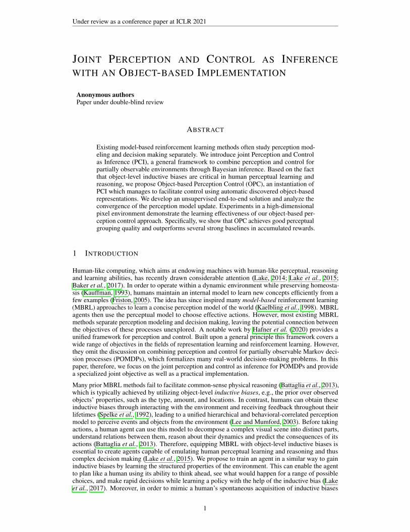
Figure 1: The graphical model of joint Perception and Control as Inference (PCI), where s and orepresent the latent state and the binary optimality binary variable, respectively. The hierarchicalperception model includes a bottom-up recognition model q(s) and a top-down generative modelp(x, o, s) (decomposed into the likelihood p(x, o|s) and the prior belief p(s)). Control is performedby taking an action a to affect the environment state.

throughout its life, we propose to build a model able to acquire new knowledge online, rather than aone which merely generates static information from offline training (Dehaene et al., 2017).

In this paper, we introduce joint Perception and Control as Inference (PCI) as shown in Fig. (1), aunified framework for decision making and perception modeling to facilitate understanding of theenvironment while providing a joint objective for both the perception and the action choice. As weargue that inductive bias gained in object-based perception is beneficial for control tasks, we thenpropose Object-based Perception Control (OPC), an instantiation of PCI which facilitates control withthe help of automatically discovered representations of objects from raw pixels. We consider a settinginspired by real-world scenarios; we consider a partially observable environment in which agents’observations consist of a visual scene with compositional structure. The perception optimization ofOPC is typically achieved by inference in a spatial mixture model through generalized expectationmaximization (Dempster et al., 1977), while the policy optimization is derived from conventionaltemporal-difference (TD) learning (Sutton, 1988). Proof of convergence for the perception modelupdate is provided in Appendix A. We test OPC on the Pixel Waterworld environment. Our resultsshow that OPC achieves good quality and consistent perceptual grouping and outperforms severalstrong baselines in terms of accumulated rewards.

2 RELATED WORK

Connecting Perception and Control Formulating RL as Bayesian inference over inputs andactions has been explored by recent works (Todorov, 2008; Kappen et al., 2009; Rawlik et al., 2010;Ortega and Braun, 2011; Levine, 2018; Tschiatschek et al., 2018; Lee et al., 2019b;a; Ortega etal., 2019; Xin et al., 2020; O’Donoghue et al., 2020). The generalized free energy principle (Parrand Friston, 2019) studies a unified objective by heuristically defining entropy terms. A unifiedframework for perception and control from a general principle is proposed by Hafner et al. (2020).Their framework provides a common foundation from which a wide range of objectives can be derivedsuch as representation learning, information gain, empowerment, and skill discovery. However, onetrade-off for the generality of their framework is the loss in precision. Environments in manyreal-world decision-making problems are only partially observable, which signifies the importanceof MBRL methods to solving POMDPs. However, relevant and integrated discussion is omittedin Hafner et al. (2020). In contrast, we focus on the joint perception and control as inference forPOMDPs and provide a specialized joint-objective as well as a practical implementation.

Model-based Deep Reinforcement Learning MBRL algorithms have been shown to be effectivein various tasks (Gu et al., 2016), including operating in environments with high-dimensional rawpixel observations (Igl et al., 2018; Shani et al., 2005; Watter et al., 2015; Levine et al., 2016; Finnand Levine, 2017). Existing methods have considered incorporating reward structure into model-learning (Farahmand et al., 2017; Oh et al., 2017), while our proposed PCI takes one step forward byincorporating the perception model into the control-as-inference derivation to yield a single unifiedobjective for multiple components in a pipeline. One of the methods closely related to OPC is theWorld Model (Ha and Schmidhuber, 2018), which consists of offline and separately trained modelsfor vision, memory, and control. These methods typically produce entangled latent representationsfor pixel observations whereas, for real world tasks such as reasoning and physical interaction, itis often necessary to identify and manipulate multiple entities and their relationships for optimalperformance. Although Zambaldi et al. (2018) has used the relational mechanism to discover andreason about entities, their model needs additional supervision of location information.

2


Object-based Reinforcement Learning The object-based approach, which recognizes decom-posed objects from the environment observations, has attracted considerable attention in RL aswell (Schmidhuber, 1992). However, most models often use pre-trained object-based representationsrather than learning them from high-dimensional observations (Diuk et al., 2008; Kansky et al.,2017). When objects are extracted through learning methods, these models usually require supervisedmodeling of the object property, by either comparing the activation spectrum generated from neuralnetwork filters with existing types (Garnelo et al., 2016) or leveraging the bounding boxes generatedby standard object detection algorithms (Keramati et al., 2018). MOREL (Goel et al., 2018) appliesoptical flow in video sequences to learn the position and velocity information as input for model-freeRL frameworks.

A distinguishing feature of our work in relation to previous works in MBRL and the object-based RLis that we provide the decision-making process with object-based abstractions of high-dimensionalobservations in an unsupervised manner, which contribute to faster learning.

Unsupervised Object Segmentation Unsupervised object segmentation and representation learn-ing have seen several recent breakthroughs, such as IODINE (Greff et al., 2019), MONet (Burgess etal., 2019), and GENESIS (Engelcke et al., 2020). Several recent works have investigated the unsu-pervised object extraction for reinforcement learning as well (Zhu et al., 2018; Asai and Fukunaga,2017; Kulkarni et al., 2019; Watters et al., 2019; Veerapaneni et al., 2020). Although OPC is builtupon a previous unsupervised object segmentation back-end (Greff et al., 2017; van Steenkiste etal., 2018), we explore one step forward by proposing a joint framework for perceptual groupingand decision-making. This could help an agent to discover structured objects from raw pixels sothat it could better tackle its decision problems. Our framework also adheres to the Bayesian brainhypothesis by maintaining and updating a compact perception model towards the cause of particularobservations (Friston, 2010).

3 METHODS

We start by introducing the environment as a partially observable Markov Decision Process (POMDP)with an object-based observation distribution in Sect. 3.11. We then introduce PCI, a generalframework for joint perception and control as inference in Sect. 3.2 and arrive at a joint objective forperception and control models. In the remainder of this section we propose OPC, a practical methodto optimize the joint objective in the context of an object-based environment, which requires themodel to exploit the compositional structure of a visual scene.

3.1 ENVIRONMENT SETTING

We define the environment as a POMDP represented by the tuple � = hS,P,A,X ,U ,Ri, whereS,A,X are the state space, the action space, and the observation space, respectively. At time step t,we consider an agent’s observation xt 2 X ⌘ RD as a visual image (a matrix of pixels) composited ofK objects, where each pixel xi is determined by exactly one object. The agent receives xt followingthe conditional observation distribution U(xt|st) : S ! X , where the hidden state st is definedby the tuple (zt,✓t1, . . . ,✓

tK). Concretely, we denote as zt 2 Z ⌘ [0, 1]D⇥K the latent variable

which encodes the unknown true pixel assignments, such that zti,k = 1 iff pixel zti was generated bycomponent k. Each pixel xt

i is then rendered by its corresponding object representations ✓tk 2 RM

through a pixel-wise distribution U ti,k(xt

i|zti,k = 1) 2, where ti,k = f�(✓tk)i is generated by feeding

✓tk into a differentiable non-linear function f�. When the environment receives an action at 2 A, itmoves to a new state st+1 following the transition function P(st+1|st, at) : S⇥A ! S . We assumethe transition function could be parameterized and we integrate its parameter into �. To embed thecontrol problem into the graphical model, we also introduce an additional binary random variable ot

to represent the optimality at time step t, i.e., ot = 1 denotes that time step t is optimal, and ot = 0denotes that it is not optimal. We choose the distribution over ot to be p(ot = 1|st, at) / exp(rt),

1Note that the PCI framework is designed for general POMDPs. We extend Sect. 3.1 to object-basedPOMDPs for the purpose of introducing the environment setting for OPC.

2We consider U as Gaussian, i.e., U ti,k

(xti|zti,k = 1) ⇠ N (xt

i;µ = ti,k,�

2) for some fixed �2.

3


where rt 2 R is the observed reward provided by the environment according to the reward functionR(rt|st, at) : S ⇥A ! R. We denote the distribution over initial state as p(s1) : S ! [0, 1].

3.2 JOINT PERCEPTION AND CONTROL AS INFERENCE

To formalize the belief about the unobserved hidden cause of the history observation xt, the agentmaintains a perception model qw(s) to approximate the distribution over latent states as illustratedin Fig. (1). An agent’s inferred belief about the latent state could serve as a sufficient statistic ofthe history and be used as input to its policy ⇡, which guides the agent to act in the environment.The goal of the agent is to maximize the future optimality o�t while learning a perception model byinferring unobserved temporal hidden states given the past observations xt and actions at, whichis achieved by maximizing the following objective:

log p(o�t,xt|a<t) = logX

s�1,a�t,x>t

p(o�t, s�1,x�1, a�t|a<t)

= log

2

4X

st

qwQt

j=1 p(xj |sj)p(s1)

Qt�1m=1 p(s

m+1|sm, am)

qw[ 1�]

3

5 , (1)

where we denote qw.= q(st|xt, a<t) and use 1� to represent the term related to control as

1� =X

s>t,a�t,x>t

Y

n=t

p(on|sn, an)Y

k=t

p(xk+1|sk+1)p(sk+1|sk, ak)p(ak|a<t).

The full derivation is presented in Appendix C.1. We denote qw.= q(st|xt, a<t) and assume

qw = p(s1)Qt

g=2 q(sg|x<g, a<g), where we slightly abuse notation for qw by ignoring the fact that

we sample from the model p(s1) for t = 1. We then apply Jensen’s inequality to Eq.(1) and get

log p(o�t,xt|a<t) � Est⇠qw

"log

Qtj=1 p(x

j |sj)p(s1)Qt�1

m=1 p(sm+1|sm, am)

p(s1)Qt

g=2 q(sg|x<g, a<g)

#+ Est⇠qw [log 1�]

=Est⇠qw

"log

tY

j=1

p(xj |sj)

#�DKL

"t�1Y

g=1

q(sg+1|xg, ag)kp(sg+1|sg, ag)

#

| {z }Lw(qw,�)

+Est⇠qw [log 1�] ,

where DKL represents the Kullback–Leibler divergence (Kullback and Leibler, 1951). As intro-duced in Sect. 3.1, we parameterize the transition distribution p�(st+1|st, at) and the observationdistribution p�(xt|st) by �. An instantiation to optimize the above evidence lower bound (ELBO)Lw(qw,�) in an environment with explicit physical properties and high-dimensional pixel-levelobservations will be discussed in Sect. 3.3.

We now derive the control objective by extending 1� as

logX

s>t,a�t,x>t

q(s>t, a�t,x>t)

Qn=t p(o

n|sn, an)Q

k=t p�(xk+1|sk+1)p�(s

k+1|sk, ak)p(ak|a<t)

q(s>t, a�t,x>t)

where we assume q(s>t, a�t,x>t) =Q

h=t p�(xh+1|sh+1)p�(sh+1|sh, ah)⇡(ah|sh) and denote

qc.= q(s>t, a�t,x>t). We then apply Jensen’s inequality to Est⇠qw [log 1�] and get

Est⇠qw [log 1�] �Est⇠qw

2

4X

s>t,a�t,x>t

qc log

Qn=t p(o

n|sn, an)Q

k=t p�(xk+1|sk+1)p�(sk+1|sk, ak)p(ak|a<t)Q

h=t p�(xh+1|sh+1)p�(sh+1|sh, ah)⇡(ah|sh)

3

5

=Est⇠qw

"X

t

Est+1,at,xt+1⇠⇢�⇡⇥R(st, at)�DKL(⇡(a

t|st)||p(at|a<t))⇤#,

(2)where we denote ⇢� as p�(xh+1|sh+1)p�(sh+1|sh, ah). Note that as this control objective is anexpectation under ⇢�, reward maximization also bias the learning of our perception model. We willpropose an option to optimize the control objective Eq.(2) in Sect. 3.4.

4


3.3 OBJECT-BASED PERCEPTION MODEL UPDATE

We now introduce OPC, an instantiation of PCI in the context of an object-based environment.Following the generalized expectation maximization (Dempster et al., 1977), we optimize the ELBOLw(qw,�) by improving the perception model qw about the true posterior p�(st+1|xt+1, st, at) withrespect to a set of object representations ✓t = [✓t1, . . . ,✓

tK ] 2 ⌦ ⇢ RM⇥K .

E-step to compute a new estimate qw of the posterior. Assume the ELBO is already maximizedwith respect to qw at time step t, i.e., qw = p�(s

t+1i |xt+1

i , st, at) = p�(zt+1i |xt+1

i , ti , a

t), we cangenerate a soft-assignment of each pixel to one of the K objects as

⌘ti,k.= p�(z

t+1i,k = 1|xt+1

i , ti , a

t). (3)

M-step to update the model parameter �. We then find ✓t+1 to maximize the ELBO as✓t+1 = argmax

✓t+1E

zt+1⇠⌘t

⇥log p�(x

t+1, zt+1, t+1|st, at)⇤ .= argmax

✓t+1⇤✓t(✓t+1). (4)

See derivation in Appendix C.2. Note that Eq. (4) returns a set of points that maximize ⇤✓t(✓t+1),and we choose ✓t+1 to be any value within this set. To update the perception model by maximizingthe evidence lower bound with respect to q(st) and ✓t+1, we compute Eq. (3) and Eq. (4) iteratively.However, an analytical solution to Eq. (4) is not available because we use a differentiable non-linearfunction f� to map from object representations ✓tk into t

i,k = f�(✓tk)i. Therefore, we get ✓t+1k by

✓t+1k = ✓tk + ↵

@⇤✓t+1(✓t+2)

@✓t+1k

��✓t+1k =✓t

k

= ✓tk + ↵DX

i=1

⌘ti,k · ti,k � xt+1

i

�2·@ t

i,k

@✓tk, (5)

where ↵ is the learning rate (see details of derivation in Appendix C.3).

We regard the iterative process as a tro-step rollout of K copies of a recurrent neural net-work with hidden states ✓tk receiving ⌘t

k � ( tk � xt+1) as input (see the inner loop of Algo-

rithm 1). Each copy generates a new t+1k , which is then used to re-estimate the soft-assignments

⌘t+1k . We parameterize the Jacobian @ t

k/@✓tk and the differentiable non-linear function f�k

using a convolutional encoder-decoder architecture with a recurrent neural network bottleneck,

ηtψ t

θ t+1Rel

MLP

Vζvt+1

πζt+1

TD-error

Env rt+1

K {

ψ t+1

DDDD

ηt+1

— *

Decision Making ModulePerception Model

gradient flow

Food Agent Poison

xt+1

xt+2

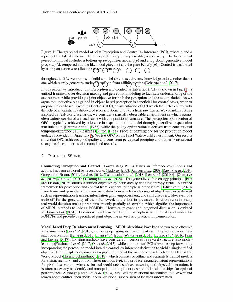
Figure 2: Illustration of OPC and the Pixel Waterworld envi-ronment. We regard the perception update as K copies of anRNN with hidden states ✓tk receiving ⌘t

k � ( tk � xt+1) as input.

Each copy generates a new t+1k , which is used to re-estimate

the soft-assignments ⌘t+1k for the calculation of the expected

log-likelihood ⇤✓t+1(✓t+2). The hidden states are then used asthe input to decision-making (before being fed into an optionalrelational module) to guide the agent’s action.

which linearly combines the out-put of the encoder with ✓tk fromthe previous time step. To fit thestatistical model f� to capturethe regularities corresponding tothe observation and the transitiondistribution for given POMDPs,we back-propagate the gradientof E⌧⇠⇡

⇥⇤✓t(✓t+1)

⇤through

“time” (also known as theBPTT Werbos (1988)) into theweights �. We demonstratethe convergence of a sequenceof {Lw

✓t(qw,�)} generated bythe perception update in Ap-pendix A. The proof is presentedby showing that the learningprocess follows the Global Con-vergence Theorem (Zangwill,1969).

Our implementation of the per-ceptual model is based on the un-supervised perceptual groupingmethod proposed by (Greff et al.,2017; van Steenkiste et al., 2018). However, using other advanced unsupervised object representationslearning methods as the perceptual model (such as IODINE (Greff et al., 2019) and MONet (Burgesset al., 2019)) is a straightforward extension.

5


Algorithm 1 Learning the Object-based Perception ControlInitialize ✓,⌘,�, ⇣, ⇣v, Tepi, tro, KCreate Ne environments that will execute in parallelwhile training not finished do

Initialize the history Da,Dx,D⌘ with environment rollouts for tro +1 time-steps under current policy ⇡⇣for T = 1 to Tepi � tro do

d� 0Get ⌘T�1 from D⌘

for t = T to T + tro doGet at,xt from Da,Dx respectivelyFeed ⌘t�1

k � ( t�1k � xt) into each of the K RNN copy to get ✓tk and forward-output t

k

Compute ⌘tk by Eq. 3

d� d�+ @��⇤✓t(✓t+1)

�/@� by Eq. (4)

Perform aT+tro according to policy ⇡⇣(aT+tro |✓T+tro)Receive reward rT+tro and new observation xT+tro+1

Store aT+tro ,xT+tro+1,⌘T in Da,Dx,D⌘ respectivelyFeed ⌘T+tro

k � ( T+trok � xT+tro+1) into each of the K RNN copy to get ✓T+tro+1

k

y rT+tro + �V⇣v (✓T+tro+1)

d⇣ r⇣ log ⇡⇣(aT+tro |✓T+tro)(y � V⇣v (✓T+tro))

d⇣v @�y � V⇣v (✓

T+tro)�2/@⇣v

d� d�+ @�y � V⇣v (✓

T+tro)�2/@�

Perform synchronous update of � using d�, of ⇣ using d⇣, and of ⇣v using d⇣v

3.4 DECISION-MAKING MODULE UPDATE

Recall that the control objective in Eq.(2) is the sum of the expected total reward along trajectory ⇢✓⇡and the negative KL divergence between the policy and our prior about the future actions. The priorcan reflect a preference over policies. For example, a uniform prior in SAC (Haarnoja et al., 2018)corresponds to the preference for a simple policy with minimal assumptions. This could preventearly convergence to sub-optimal policies. However, as we focus on studying the benefit of combingperception with control, we do not pre-impose a preference for policies. Therefore we set the priorequal to our training policy, resulting in a zero KL divergence term in the objective.

To maximize the total reward along trajectory ⇢✓⇡, we follow the conventional temporal-difference(TD) learning approach (Sutton, 1988) by feeding the object abstractions into a small multilayerperceptron (MLP) (Rumelhart et al., 1986) to produce a (dimR(A) + 1)-dimensional vector, whichis split into a dimR(A)-dimensional vector of ⇡⇣’s (the ‘actor’) logits, and a baseline scalar V⇣v(the ‘critic’). The ⇡⇣ logits are normalized using a softmax function, and used as the multinomialdistribution from which an action is sampled. The V⇣v is an estimate of the state-value function at thecurrent state, which is given by the last hidden state ✓ of the tro-step RNN rollout. On training thedecision-making module, the V⇣v is used to compute the temporal-difference error given by

LTD = (yt+1 � V⇣v (✓t+1))2, yt+1 = rt+1 + �V⇣v (✓

t+2), (6)

where � 2 [0, 1) is a discount factor. LTD is used both to optimize ⇡⇣ to generate actions with largertotal rewards than V⇣v predicts by updating ⇣ with respect to the policy gradient

r⇣ log ⇡⇣(at+1|✓t+1)(y � V⇣v (✓t+1)),

and to optimize V⇣v to more accurately estimate state values by updating ⇣v. Also, differentiatingLTD with respect to � enables the gradient-based optimizers to update the perception model. Weprovide the pseudo-code for one-step TD-learning of the proposed model in Algorithm 1. By groupingobjects concerning the reward, our model distinguishes objects with visual similarities but differentsemantics, thus helping the agent to better understand the environment.

4 EXPERIMENTS

4.1 PIXEL WATERWORLD

We demonstrate the advantage of unifying decision making and perception modeling by applyingOPC on an environment similar to the one used in COBRA (Watters et al., 2019), a modified

6


Waterworld environment (Karpathy, 2015), where the observations are 84⇥ 84 grayscale raw pixelimages composited of an agent and two types of randomly moving targets: the poison and the food,as illustrated in Fig. (2). The agent can control its velocity by choosing from four available actions: toapply the thruster to the left, right, up and down. A negative cost is given to the agent if it touches anypoison target, while a positive reward for making contact with any food target. The optimal strategydepends on the number, speed, and size of objects, thus requiring the agent to infer the underlyingdynamics of the environment within a given amount of observations.

The intuition of this environment is to test whether the agent can quickly learn dynamics of a newenvironment online without any prior knowledge, i.e., the execution-time optimization throughout theagent’s life-cycle to mimic humans’ spontaneous process of obtaining inductive biases. We chooseAdvantage Actor-Critic (A2C) (Mnih et al., 2016) as the decision-making module of OPC withoutloss of generality, although other online learning methods are also applicable. For OPC, we useK = 4 and tro = 20 except for Sect. 4.5, where we analyze the effect of the hyper-parameter setting.

4.2 ACCUMULATED REWARD COMPARISONS

0 1 2 3 4 5# of experienced observations (*1e5)

−20

−10

0

Costs (*1e3)

A2C, th 1A2C, th 4W0-A2C23C

(a)

0 1 2 3 4 5# of experienced observations (*1e5)

−1.5

−1.0

−0.5

0.0

3eriod Costs (*1e3)

5andoPA2C, th 1

A2C, th 4W0-A2C

23C

(b)

0 1 2 3 4 5# Rf experienced RbservatiRns (*1e5)

−1.5

−1.0

−0.5

0.0

3eriRd CRsts (*1e3)

. 4

. 4, 5el

. 3

. 3, 5el

(c)

0 1 2 3 4 5# Rf experienced RbservatiRns (*1e5)

−1.5

−1.0

−0.5

0.0

3er

iRd

CRs

ts (*

1e3)

tRO=20tRO=20, 5eltRO=10tRO=10, 5el

(d)Figure 3: Performance comparisons between methods.

To verify object-level in-ductive biases facilitatingdecision making, we com-pare OPC against a setof baseline algorithms, in-cluding: 1) the standardA2C, which uses convo-lutional layers to trans-form the raw pixel ob-servations to low dimen-sional vectors as input forthe same MLP describedin Sect. 3.4, 2) the WorldModel (Ha and Schmid-huber, 2018) with A2Cfor control (WM-A2C),a state-of-the-art model-based approach, whichseparately learns a vi-sual and a memorizationmodel to provide the in-put for a standard A2C, and 3) the random policy. For both the baseline A2C, WM-A2C and thedecision-making module of OPC, we follow the convention of Mnih et al. (2016) by running thealgorithm in the forward view and using the same mix of n-step returns to update both ⇡⇣ andV⇣v . Details of the model and of hyperparameter setting can be found in Appendix B. We build theenvironment with two poison objects and one food object, and set the size of the agent 1.5 timessmaller than the target. Results are reported with the average value among separate runs of threerandom seeds. Note that the training procedure of WM-A2C includes independent off-line trainingfor each component, thus requiring many more observation samples than OPC. Following its originalearly-stopping criteria, we report that WM-A2C requires 300 times more observation samples forseparately training a perception model before learning a policy to give the results presented in Fig. (3).

Fig. (3a) shows the result of accumulated rewards after each agent has experienced the same amountof observations. Note that OPC uses the plotted number of experienced observations for trainingthe entire model, while WM-A2C uses the amount of observations only for training the controlmodule. It is clear that the agent with OPC achieves the greatest performance, outperforming allother agents regardless of model in terms of accumulated reward. We believe this advantage isdue to the object-level inductive biases obtained by the perception model (compared to entangledrepresentations extracted by the CNN used in standard A2C), and the unified learning of perceptionand control of OPC (as opposed to the separate learning of different modules in WM-A2C).

To illustrate each agent’s learning process through time, we also present the period reward, whichis the accumulated reward during a given period of environment interactions (2e4 of experienced

7


observations). As illustrated in Fig. (3b), OPC significantly improves the sample efficiency of A2C,which enables the agent acting in the environment to find an optimal strategy more quickly thanagents with baseline models. We also find that the standard version of A2C with four parallel threadsgives roughly the same result as the single-threaded version of A2C (the same as the decision-makingmodule of OPC), eliminating the potential drawback of single-thread learning.

4.3 PERCEPTUAL GROUPING RESULTS

To demonstrate the performance of the perception model, we provide an example rollout at theearly stage of training in Fig. (4). We assign a different color to each k for better visualization

Figure 4: A sample rollout of perceptual groupingby OPC. The observation (top row), the next-stepprediction k of each copy of the K RNN copy(rows 4 to 7), the

Pk k (row 2), and the soft-

assignment ⌘ of the pixels to each of the copies(row 3). We assign a different color to each k

for better visualization. This sample rollout showsthat all objects are grouped semantically.

and show through the soft-assignment ⌘ thatall objects are grouped semantically: the agentin blue, the food in green, and both poisonsin red. During the joint training of perceptionand policy, the soft-assignment gradually consti-tutes a semantic segmentation as the TD signalimproves the recognition when grouping pixelsinto different types based on the interaction withthe environment. Consequently, the learned ob-ject representations ✓ becomes a semantic inter-pretation of raw pixels grouped into perceptualobjects.

4.4 BENEFITS OF JOINT INFERENCE

To gain insights into the benefit of the controlobjective for joint inference, we further compareOPC against OP, a perception model with thesame architecture as OPC but no guidance ofthe TD signal from RL, i.e., using the sameunsupervised object segmentation back-end asin Greff et al. (2017). Fig. (5) shows the result of accumulated rewards and the soft-assignment ⌘produced by both perception models. Results are produced by models running in environments withthe same random seed.

As illustrated in Fig. (5a), OPC outperforms OP in terms of the accumulated rewards throughtime with a given amount of observations. This performance difference owes to the fact shownin Fig. (5b), where the ⌘ of OP are overlaid, and the shapes are not delineated in bold colorsbut are a mixture, showing that OP has not learned to segment the objects clearly. The pixelassignment (coloring) does not appear to converge even after an extremely large number of iterations,suggesting that OP alone cannot properly show signs of any semantic adaptation to the task at hand.

0.0 0.5 1.0 1.5# of experienced observations (*1e5)

−6

−4

−2

0

Cos

ts (*

1e3)

23C23

(a)OPC OP OPC OP

# = 14000 # = 14500

OPC OP OPC OP

# = 14000 # = 14500

x

(b)

Figure 5: (a) Performance comparison between OPC and OP. (b) The soft-assignment ⌘ after experiencing 14000 and 14500 observations. Each k

is assigned with a different color as in Fig. (4). x is the binary-processedoriginal observation.

On the other hand, thequality and consistency ofthe soft-assignment gen-erated by OPC are im-proved with the TD sig-nal, suggesting that RLfacilitates the learningof the perception model.Furthermore, the inter-action between objectsshown in Fig. (5b) demon-strates the agent is mov-ing away from the poison(even when the food isnearby). Because of the

environment setting of the high moving speed, larger target sizes and more poison objects, we believethat agents are given strong indications to stay away from all stimuli. Thus, the result shows anunderstanding of visual reasoning that the agent can separate itself from the rest of the objects.

8


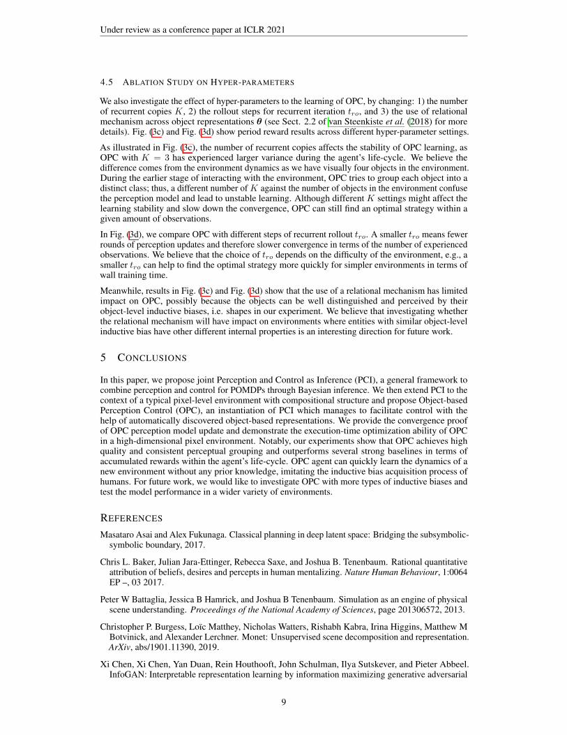
4.5 ABLATION STUDY ON HYPER-PARAMETERS

We also investigate the effect of hyper-parameters to the learning of OPC, by changing: 1) the numberof recurrent copies K, 2) the rollout steps for recurrent iteration tro, and 3) the use of relationalmechanism across object representations ✓ (see Sect. 2.2 of van Steenkiste et al. (2018) for moredetails). Fig. (3c) and Fig. (3d) show period reward results across different hyper-parameter settings.

As illustrated in Fig. (3c), the number of recurrent copies affects the stability of OPC learning, asOPC with K = 3 has experienced larger variance during the agent’s life-cycle. We believe thedifference comes from the environment dynamics as we have visually four objects in the environment.During the earlier stage of interacting with the environment, OPC tries to group each object into adistinct class; thus, a different number of K against the number of objects in the environment confusethe perception model and lead to unstable learning. Although different K settings might affect thelearning stability and slow down the convergence, OPC can still find an optimal strategy within agiven amount of observations.

In Fig. (3d), we compare OPC with different steps of recurrent rollout tro. A smaller tro means fewerrounds of perception updates and therefore slower convergence in terms of the number of experiencedobservations. We believe that the choice of tro depends on the difficulty of the environment, e.g., asmaller tro can help to find the optimal strategy more quickly for simpler environments in terms ofwall training time.

Meanwhile, results in Fig. (3c) and Fig. (3d) show that the use of a relational mechanism has limitedimpact on OPC, possibly because the objects can be well distinguished and perceived by theirobject-level inductive biases, i.e. shapes in our experiment. We believe that investigating whetherthe relational mechanism will have impact on environments where entities with similar object-levelinductive bias have other different internal properties is an interesting direction for future work.

5 CONCLUSIONS

In this paper, we propose joint Perception and Control as Inference (PCI), a general framework tocombine perception and control for POMDPs through Bayesian inference. We then extend PCI to thecontext of a typical pixel-level environment with compositional structure and propose Object-basedPerception Control (OPC), an instantiation of PCI which manages to facilitate control with thehelp of automatically discovered object-based representations. We provide the convergence proofof OPC perception model update and demonstrate the execution-time optimization ability of OPCin a high-dimensional pixel environment. Notably, our experiments show that OPC achieves highquality and consistent perceptual grouping and outperforms several strong baselines in terms ofaccumulated rewards within the agent’s life-cycle. OPC agent can quickly learn the dynamics of anew environment without any prior knowledge, imitating the inductive bias acquisition process ofhumans. For future work, we would like to investigate OPC with more types of inductive biases andtest the model performance in a wider variety of environments.

REFERENCES

Masataro Asai and Alex Fukunaga. Classical planning in deep latent space: Bridging the subsymbolic-symbolic boundary, 2017.

Chris L. Baker, Julian Jara-Ettinger, Rebecca Saxe, and Joshua B. Tenenbaum. Rational quantitativeattribution of beliefs, desires and percepts in human mentalizing. Nature Human Behaviour, 1:0064EP –, 03 2017.

Peter W Battaglia, Jessica B Hamrick, and Joshua B Tenenbaum. Simulation as an engine of physicalscene understanding. Proceedings of the National Academy of Sciences, page 201306572, 2013.

Christopher P. Burgess, Loïc Matthey, Nicholas Watters, Rishabh Kabra, Irina Higgins, Matthew MBotvinick, and Alexander Lerchner. Monet: Unsupervised scene decomposition and representation.ArXiv, abs/1901.11390, 2019.

Xi Chen, Xi Chen, Yan Duan, Rein Houthooft, John Schulman, Ilya Sutskever, and Pieter Abbeel.InfoGAN: Interpretable representation learning by information maximizing generative adversarial

9


nets. In D. D. Lee, U. V. Luxburg, I. Guyon, and R. Garnett, editors, Advances In NeuralInformation Processing Systems 29, pages 2172–2180. Curran Associates, Inc., 2016.

Stanislas Dehaene, Hakwan Lau, and Sid Kouider. What is consciousness, and could machines haveit? Science, 358(6362):486–492, 2017.

Arthur P Dempster, Nan M Laird, and Donald B Rubin. Maximum likelihood from incomplete datavia the em algorithm. Journal of the royal statistical society. Series B (methodological), pages1–38, 1977.

Carlos Diuk, Andre Cohen, and Michael L. Littman. An object-oriented representation for efficientreinforcement learning. In ICML, pages 240–247, 2008.

Martin Engelcke, Adam R. Kosiorek, Oiwi Parker Jones, and Ingmar Posner. GENESIS: GenerativeScene Inference and Sampling of Object-Centric Latent Representations. International Conferenceon Learning Representations (ICLR), 2020.

Amir-Massoud Farahmand, Andre Barreto, and Daniel Nikovski. Value-Aware Loss Function forModel-based Reinforcement Learning. volume 54 of Proceedings of Machine Learning Research,pages 1486–1494, Fort Lauderdale, FL, USA, 20–22 Apr 2017. PMLR.

Chelsea Finn and Sergey Levine. Deep visual foresight for planning robot motion. In Robotics andAutomation (ICRA), 2017 IEEE International Conference on, pages 2786–2793. IEEE, 2017.

Karl Friston. A theory of cortical responses. Philosophical Transactions of the Royal Society ofLondon B: Biological Sciences, 360(1456):815–836, 2005.

Karl Friston. The free-energy principle: a unified brain theory? Nature Reviews Neuroscience, 11:127EP –, 01 2010.

Marta Garnelo, Kai Arulkumaran, and Murray Shanahan. Towards deep symbolic reinforcementlearning. arXiv preprint arXiv:1609.05518, 2016.

Vikash Goel, Jameson Weng, and Pascal Poupart. Unsupervised video object segmentation for deepreinforcement learning. In NIPS, pages 5688–5699. 2018.

Klaus Greff, Sjoerd van Steenkiste, and Jürgen Schmidhuber. Neural expectation maximization. InNIPS, pages 6691–6701, 2017.

Klaus Greff, Raphaël Lopez Kaufmann, Rishabh Kabra, Nick Watters, Christopher Burgess, DanielZoran, Loic Matthey, Matthew Botvinick, and Alexander Lerchner. Multi-object representationlearning with iterative variational inference. In ICML, pages 2424–2433, 2019.

Shixiang Gu, Timothy Lillicrap, Ilya Sutskever, and Sergey Levine. Continuous deep q-learning withmodel-based acceleration. In ICML, pages 2829–2838, 2016.

David Ha and Jürgen Schmidhuber. Recurrent world models facilitate policy evolution. In NIPS,pages 2451–2463. 2018.

Tuomas Haarnoja, Aurick Zhou, Pieter Abbeel, and Sergey Levine. Soft actor-critic: Off-policymaximum entropy deep reinforcement learning with a stochastic actor. volume 80 of Proceedingsof Machine Learning Research, pages 1861–1870, Stockholmsmässan, Stockholm Sweden, 10–15Jul 2018. PMLR.

Danijar Hafner, Pedro A Ortega, Jimmy Ba, Thomas Parr, Karl Friston, and Nicolas Heess. Actionand perception as divergence minimization. arXiv preprint arXiv:2009.01791, 2020.

Maximilian Igl, Luisa Zintgraf, Tuan Anh Le, Frank Wood, and Shimon Whiteson. Deep variationalreinforcement learning for POMDPs. In ICML, pages 2117–2126, 10–15 Jul 2018.

Leslie Pack Kaelbling, Michael L Littman, and Anthony R Cassandra. Planning and acting in partiallyobservable stochastic domains. Artificial intelligence, 101(1-2):99–134, 1998.

10


Ken Kansky, Tom Silver, David A. Mély, Mohamed Eldawy, Miguel Lázaro-Gredilla, Xinghua Lou,Nimrod Dorfman, Szymon Sidor, Scott Phoenix, and Dileep George. Schema networks: Zero-shottransfer with a generative causal model of intuitive physics. In Doina Precup and Yee Whye Teh,editors, Proceedings of the 34th International Conference on Machine Learning, volume 70 ofProceedings of Machine Learning Research, pages 1809–1818, International Convention Centre,Sydney, Australia, 06–11 Aug 2017. PMLR.

Hilbert J Kappen, Vicenç Gómez, and Manfred Opper. Optimal control as a graphical model inferenceproblem. Machine learning, 87(2):159–182, 2009.

Andrej Karpathy. Reinforcejs: Waterworld. https://cs.stanford.edu/people/karpathy/reinforcejs/waterworld.html, 2015. Accessed: 2018-11-20.

Stuart A Kauffman. The origins of order: Self-organization and selection in evolution. OUP USA,1993.

Ramtin Keramati, Jay Whang, Patrick Cho, and Emma Brunskill. Strategic object oriented reinforce-ment learning. arXiv preprint arXiv:1806.00175, 2018.

Diederik P Kingma and Jimmy Ba. Adam: A method for stochastic optimization. arXiv preprintarXiv:1412.6980, 2014.

Tejas Kulkarni, Ankush Gupta, Catalin Ionescu, Sebastian Borgeaud, Malcolm Reynolds, AndrewZisserman, and Volodymyr Mnih. Unsupervised learning of object keypoints for perception andcontrol. arXiv preprint arXiv:1906.11883, 2019.

Solomon Kullback and Richard A Leibler. On information and sufficiency. The annals of mathemati-cal statistics, 22(1):79–86, 1951.

Brenden M. Lake, Ruslan Salakhutdinov, and Joshua B. Tenenbaum. Human-level concept learningthrough probabilistic program induction. Science, 350(6266):1332–1338, 2015.

Brenden M Lake, Tomer D Ullman, Joshua B Tenenbaum, and Samuel J Gershman. Buildingmachines that learn and think like people. Behavioral and Brain Sciences, 40, 2017.

Brenden M Lake. Towards more human-like concept learning in machines: Compositionality,causality, and learning-to-learn. PhD thesis, Massachusetts Institute of Technology, 2014.

Tai Sing Lee and David Mumford. Hierarchical bayesian inference in the visual cortex. JOSA A,20(7):1434–1448, 2003.

Alex X Lee, Anusha Nagabandi, Pieter Abbeel, and Sergey Levine. Stochastic latent actor-critic:Deep reinforcement learning with a latent variable model. arXiv preprint arXiv:1907.00953, 2019.

Lisa Lee, Benjamin Eysenbach, Emilio Parisotto, Eric Xing, Sergey Levine, and Ruslan Salakhutdinov.Efficient exploration via state marginal matching. arXiv preprint arXiv:1906.05274, 2019.

Sergey Levine, Chelsea Finn, Trevor Darrell, and Pieter Abbeel. End-to-end training of deepvisuomotor policies. The Journal of Machine Learning Research, 17(1):1334–1373, 2016.

Sergey Levine. Reinforcement learning and control as probabilistic inference: Tutorial and review.arXiv preprint arXiv:1805.00909, 2018.

Volodymyr Mnih, Koray Kavukcuoglu, David Silver, Alex Graves, Ioannis Antonoglou, DaanWierstra, and Martin Riedmiller. Playing atari with deep reinforcement learning. arXiv preprintarXiv:1312.5602, 2013.

Volodymyr Mnih, Adria Puigdomenech Badia, Mehdi Mirza, Alex Graves, Timothy Lillicrap, TimHarley, David Silver, and Koray Kavukcuoglu. Asynchronous methods for deep reinforcementlearning. In ICML, pages 1928–1937, 20–22 Jun 2016.

Brendan O’Donoghue, Ian Osband, and Catalin Ionescu. Making sense of reinforcement learningand probabilistic inference. In International Conference on Learning Representations, 2020.

11

https://cs.stanford.edu/people/karpathy/reinforcejs/waterworld.html

https://cs.stanford.edu/people/karpathy/reinforcejs/waterworld.html


Junhyuk Oh, Satinder Singh, and Honglak Lee. Value prediction network. In I. Guyon, U. V. Luxburg,S. Bengio, H. Wallach, R. Fergus, S. Vishwanathan, and R. Garnett, editors, Advances in NeuralInformation Processing Systems, volume 30, pages 6118–6128. Curran Associates, Inc., 2017.

Daniel Alexander Ortega and Pedro Alejandro Braun. Information, utility and bounded rationality. InInternational Conference on Artificial General Intelligence, pages 269–274. Springer, 2011.

Pedro A. Ortega, J. X. Wang, M. Rowland, Tim Genewein, Zeb Kurth-Nelson, Razvan Pascanu,N. Heess, J. Veness, A. Pritzel, P. Sprechmann, Siddhant M. Jayakumar, T. McGrath, K. Miller,Mohammad Gheshlaghi Azar, Ian Osband, Neil C. Rabinowitz, A. György, S. Chiappa, SimonOsindero, Y. Teh, H. V. Hasselt, N. D. Freitas, M. Botvinick, and S. Legg. Meta-learning ofsequential strategies. ArXiv, abs/1905.03030, 2019.

Thomas Parr and Karl J Friston. Generalised free energy and active inference. Biological cybernetics,113(5-6):495–513, 2019.

Konrad Rawlik, Marc Toussaint, and Sethu Vijayakumar. Approximate inference and stochasticoptimal control. arXiv preprint arXiv:1009.3958, 2010.

D. E. Rumelhart, G. E. Hinton, and R. J. Williams. Parallel distributed processing: Explorationsin the microstructure of cognition, vol. 1. chapter Learning Internal Representations by ErrorPropagation, pages 318–362. MIT Press, Cambridge, MA, USA, 1986.

Jürgen Schmidhuber. Learning factorial codes by predictability minimization. Neural Computation,4(6):863–879, 1992.

Guy Shani, Ronen I. Brafman, and Solomon E. Shimony. Model-based online learning of pomdps.In Machine Learning: ECML 2005, pages 353–364, Berlin, Heidelberg, 2005. Springer BerlinHeidelberg.

Elizabeth S Spelke, Karen Breinlinger, Janet Macomber, and Kristen Jacobson. Origins of knowledge.Psychological review, 99(4):605, 1992.

Richard S. Sutton. Learning to predict by the methods of temporal differences. Machine Learning,3(1):9–44, Aug 1988.

Tijmen Tieleman and Geoffrey Hinton. Lecture 6.5-rmsprop: Divide the gradient by a runningaverage of its recent magnitude. COURSERA: Neural networks for machine learning, 4(2):26–31,2012.

Emanuel Todorov. General duality between optimal control and estimation. In 2008 47th IEEEConference on Decision and Control, pages 4286–4292. IEEE, 2008.

Sebastian Tschiatschek, Kai Arulkumaran, Jan Stühmer, and Katja Hofmann. Variational inferencefor data-efficient model learning in pomdps. arXiv preprint arXiv:1805.09281, 2018.

Sjoerd van Steenkiste, Michael Chang, Klaus Greff, and Jürgen Schmidhuber. Relational neuralexpectation maximization: Unsupervised discovery of objects and their interactions. In ICLR,2018.

Rishi Veerapaneni, John D. Co-Reyes, Michael Chang, Michael Janner, Chelsea Finn, Jiajun Wu,Joshua Tenenbaum, and Sergey Levine. Entity abstraction in visual model-based reinforcementlearning. In Leslie Pack Kaelbling, Danica Kragic, and Komei Sugiura, editors, Proceedings of theConference on Robot Learning, volume 100 of Proceedings of Machine Learning Research, pages1439–1456. PMLR, 30 Oct–01 Nov 2020.

Manuel Watter, Jost Springenberg, Joschka Boedecker, and Martin Riedmiller. Embed to control:A locally linear latent dynamics model for control from raw images. In Advances in neuralinformation processing systems, pages 2746–2754, 2015.

Nicholas Watters, Loic Matthey, Matko Bosnjak, Christopher P Burgess, and Alexander Lerchner.Cobra: Data-efficient model-based rl through unsupervised object discovery and curiosity-drivenexploration. arXiv preprint arXiv:1905.09275, 2019.

12


Paul J. Werbos. Generalization of backpropagation with application to a recurrent gas market model.Neural Networks, 1(4):339 – 356, 1988.

CF Jeff Wu. On the convergence properties of the em algorithm. The Annals of statistics, pages95–103, 1983.

Bo Xin, Haixu Yu, You Qin, Qing Tang, and Zhangqing Zhu. Exploration entropy for reinforcementlearning. Mathematical Problems in Engineering, 2020, 2020.

Vinícius Flores Zambaldi, David Raposo, Adam Santoro, Victor Bapst, Yujia Li, Igor Babuschkin,Karl Tuyls, David P. Reichert, Timothy P. Lillicrap, Edward Lockhart, Murray Shanahan, VictoriaLangston, Razvan Pascanu, Matthew Botvinick, Oriol Vinyals, and Peter W. Battaglia. Relationaldeep reinforcement learning. CoRR, abs/1806.01830, 2018.

Willard I Zangwill. Nonlinear programming: a unified approach, volume 196. Prentice-HallEnglewood Cliffs, NJ, 1969.

Guangxiang Zhu, Zhiao Huang, and Chongjie Zhang. Object-oriented dynamics predictor. In NIPS,pages 9826–9837. 2018.

13


A CONVERGENCE OF THE OBJECT-BASED PERCEPTION MODEL UPDATE

Under main assumptions and lemmas as introduced below, we demonstrate the convergence of asequence of {Lw

✓t(qw,�)} generated by the perception update. The proof is presented by showingthat the learning process follows the Global Convergence Theorem (Zangwill, 1969).Assumption 1. ⌦✓0 =

�✓ 2 ⌦ : Lw

✓ (qw,�) Lw

✓0(qw,�)

is compact for any Lw✓0(qw,�) < 1.

Assumption 2. L is continuous in ⌦ and differentiable in the interior of ⌦.

The above assumptions lead to the fact that {Lw✓t(qw,�)} is bounded for any ✓0 2 ⌦.

Lemma 1. Let ⌦S be the set of stationary points in the interior of ⌦, then the mappingargmax✓t+1 ⇤✓t(✓t+1) from Eq. 4 is closed over ⌦\⌦S (the complement of ⌦S).

Proof. See Wu (1983). A sufficient condition is that ⇤✓t(✓t+1) is continuous in both ✓t+1 and✓t.

Proposition 1. Let ⌦S be the set of stationary points in the interior of ⌦, then (i.) 8✓t 2⌦S ,Lw

✓t+1(qw,�) Lw✓t(qw,�) and (ii.) 8✓t 2 ⌦\⌦S ,Lw

✓t+1(qw,�) < Lw✓t(qw,�).

Proof. Note that (i.) holds true given the condition. To prove (ii.), consider any ✓t 2 ⌦\⌦S , we have

@Lw✓t(qw,�)

@✓t+1

��✓t+1=✓t

=@⇤✓t(✓t+1)

@✓t+1

��✓t+1=✓t

6= 0.

Hence ⇤✓t(✓t+1) is not maximized at ✓t+1 = ✓t. Given the perception update described by Eq. (5),we therefore have ⇤✓t(✓t+1) > ⇤✓t(✓t), which implies Lw

✓t+1(qw,�) < Lw✓t(qw,�).

Theorem 1. Let {✓t} be a sequence generated by the mapping from Eq. 4, ⌦S be the set of stationarypoints in the interior of ⌦. If Assumptions 1 & 2, Lemma 1, and Proposition 1 are met, then all thelimit points of {✓t} are stationary points (local minima) and Lw

✓t(qw,�) converges monotonically toJ⇤ = Lw

✓⇤(qw,�) for some stationary point ✓⇤ 2 ⌦S .

Proof. Suppose that ✓⇤ is a limit point of the sequence {✓t}. Given Assumptions 1 & 2 andProposition 1.i), we have that the sequence {✓t} are contained in a compact set ⌦K ⇢ ⌦. Thus, thereis a subsequence {✓l}l2L of {✓t} such that ✓l ! ✓⇤ as l ! 1 and l 2 L.

We first show that Lw✓t(qw,�) ! Lw

✓⇤(qw,�) as t ! 1. Given L is continuous in ⌦ (Assumption2), we have Lw

✓l(qw,�) ! Lw✓⇤(qw,�) as l ! 1 and l 2 L, which means

8✏ > 0, 9l(✏) 2 L s.t. 8l � l(✏), l 2 L,Lw✓l(q

w,�)� Lw✓⇤(qw,�) < ✏. (7)

Given Proposition 1 and Eq. (4), L is therefore monotonically decreasing on the sequence {✓t}1t=0,which gives

8t,Lw✓t(qw,�)� Lw

✓⇤(qw,�) � 0. (8)Given Eq. (7), for any t � l(✏), we have

Lw✓t(qw,�)� Lw

✓⇤(qw,�) = Lw✓t(qw,�)� Lw

✓l(✏)(qw,�)

| {z }0

+Lw✓l(✏)(q

w,�)� Lw✓⇤(qw,�)

| {z }<✏

< ✏. (9)

Given Eq. (8) and Eq. (9), we therefore have Lw✓t(qw,�) ! Lw

✓⇤(qw,�) as t ! 1. We then provethat the limit point ✓⇤ is a stationary point. Suppose ✓⇤ is not a stationary point, i.e., ✓⇤ 2 ⌦\⌦S , weconsider the sub-sequence {✓l+1}l2L, which are also contained in the compact set ⌦K . Thus, thereis a subsequence {✓l0+1}l02L0 of {✓l+1}l2L such that ✓l

0+1 ! ✓⇤0

as l0 ! 1 and l0 2 L0, yieldingLw✓l0+1(q

w,�) ! Lw✓⇤0 (q

w,�) as l0 ! 1 and l0 2 L0, which gives

Lw✓⇤0 (q

w,�) = liml0!1l02L0

Lw✓l0+1(q

w,�) = limt!1t2N

Lw✓t(qw,�) = Lw

✓⇤(qw,�). (10)

On the other hand, since the mapping from Eq. (4) is closed over ⌦\⌦S (Lemma 1), and ✓⇤ 2 ⌦\⌦S ,we therefore have ✓⇤

0 2 argmax✓t+1 ⇤✓⇤(✓t+1), yielding Lw✓⇤0 (q

w,�) < Lw✓⇤(qw,�) (Proposition

1.ii), which contradicts Eq. (10).

14


B EXPERIMENT DETAILS

OPC In all experiments we trained the perception model using ADAM Kingma and Ba (2014) withdefault parameters and a batch size of 32. Each input consists of a sequence of binary 84⇥ 84 imagescontaining two poison objects (two circles) and one food object (a rectangle) that start in randompositions and move within the image for tro steps. These frames were thresholded at 0.0001 to obtainbinary images and added with bit-flip noise (p = 0.2). We used a convolutional encoder-decoderarchitecture inspired by recent GANs Chen et al. (2016) with a recurrent neural network as bottleneck,where the encoder used the same network architecture from Mnih et al. (2013) as

1. 8⇥ 8 conv. 16 ELU. stride 4. layer norm2. 4⇥ 4 conv. 32 ELU. stride 2. layer norm3. fully connected. 256 ELU. layer norm4. recurrent. 250 Sigmoid. layer norm on the output5. fully connected. 256 RELU. layer norm6. fully connected. 10⇥ 10⇥ 32 RELU. layer norm7. 4⇥ 4 reshape 2 nearest-neighbour, conv. 16 RELU. layer norm8. 8⇥ 8 reshape 4 nearest-neighbour, conv. 1 Sigmoid

We used the Advantage Actor-Critic (A2C) Mnih et al. (2016) with an MLP policy as the decisionmaking module of OPC. The MLP policy added a 512-unit fully connected layer with rectifiernonlinearity after layer 4 of the perception model. The decision making module had two set ofoutputs: 1) a softmax output with one entry per action representing the probability of selecting theaction, and 2) a single linear output representing the value function. The decision making modulewas trained using RMSProp Tieleman and Hinton (2012) with a learning rate of 7e � 4, a rewarddiscount factor � = 0.99, an RMSProp decay factor of 0.99, and performed updates after every 5actions.

A2C We used the same convolutional architecture as the encoder of the perception model of OPC(layer 1 to 3), followed by a fully connected layer with 512 hidden units followed by a rectifiernonlinearity. The A2C was trained using the same setting as the decision making module of OPC.

WM-A2C We used the same setting as Ha and Schmidhuber (2018) to separately train the V modeland the M model. The experience was generated off-line by a random policy operating in the PixelWaterworld environment. We concatenated the output of the V model and the M model as the A2Cinput, and trained A2C using the same setting as introduced above.

15


C DETAILS OF DERIVATION

C.1 DERIVATION OF EQ. (1)

logp(o�t,xt|a<t)

= logX

s�1,a�t,x>t

p(o�t, s�1,x�1, a�t|a<t)

= logX

s�1,a�t,x>t

p(o�t|s�1,x�1, a�1)p(s�1,x�1, a�1|a<t)

= logX

s�1,a�t,x>t

Y

n=t

p(on|sn, an)p(xt|s�1,x>t, a�1)p(s�1,x>t, a�1|a<t)

= logX

s�1,a�t,x>t

Y

n=t

p(on|sn, an)tY

j=1

p(xj |sj)p(x>t|s�1, a�1)p(s�1, a�1|a<t)

= logX

s�1,a�t,x>t

Y

n=t

p(on|sn, an)tY

j=1

p(xj |sj)Y

k=t+1

p(xk|sk)p(s>t|st, a�1)p(st, a�1|a<t)

= logX

s�1,a�t,x>t

Y

n=t

p(on|sn, an)tY

j=1

p(xj |sj)Y

k=t+1

p(xk|sk)Y

l=t

p(sl+1|sl, al)p(s1)t�1Y

m=1

p(sm+1|sm, am)Y

h=t

p(ah|a<t)

= log

2

6666664

X

st

tY

j=1

p(xj |sj)p(s1)t�1Y

m=1

p(sm+1|sm, am)

2

6666664

X

s>t,a�t,x>t

Y

n=t

p(on|sn, an)Y

k=t

p(xk+1|sk+1)p(sk+1|sk, ak)p(ak|a<t)

| {z }1�

3

7777775

3

7777775

= log

2

4X

st

q(st|xt, a<t)

Qtj=1 p(x

j |sj)p(s1)Qt�1

m=1 p(sm+1|sm, am)

q(st|xt, a<t)[ 1�]

3

5


✓t+1 =argmax✓t+1

qw log

Qtj=1 p(x

j |sj)p(s1)Qt�1

m=1 p(sm+1|sm, am)

p(s1)Qt�1

g=1 q(sg+1|xg, ag)

= argmax✓t+1

qw logp(s1)p(x1|s1)

Qt�1j=1 p(x

j+1, sj+1|sj , aj)p(s1)

Qt�1g=1 q(s

g+1|xg, ag)

= argmax✓t+1

⌘t logp(x1|s1)

Qt�1j=1 p(x

j+1, sj+1|sj , aj)Qt�1

g=1 ⌘g+1

drop terms which are constant with respect to ✓t+1

=argmax✓t+1

Ezt+1⇠⌘t

⇥log p�(x

t+1, zt+1, t+1|st, at)⇤

.=argmax

✓t+1⇤✓t(✓t+1)

16



@⇤✓t+1(✓t+2)

@✓t+1k

=@⇤✓t+1(✓t+2)

@ t+1k

·@{ t+1

k }T

@{✓t+1k }T

=

"@⇤✓t+1(✓t+2)

@ t+11,k

. . .@⇤✓t+1(✓t+2)

@ t+1D,k

#·

2

6664

@ t+11,k

@✓t+1k

...@ t+1

D,k

@✓t+1k

3

7775

=DX

i=1

@⇤✓t+1(✓t+2)

@ t+1i,k

·@ t+1

i,k

@✓t+1k

=DX

i=1

@

@ t+1i,k

2

4X

zt+1i

p�(zt+1i |xt+1

i , ti , a

t) log p t+1i

(xt+1i , zt+1

i |st, at)

3

5 ·@ t+1

i,k

@✓t+1k

=DX

i=1

@

@ t+1i,k

2

4X

zt+1i

p�(zt+1i |xt+1

i , ti , a

t) log p t+1i

(xt+1i |zt+1

i )p(zt+1i |st, at)

3

5 ·@ t+1

i,k

@✓t+1k

=DX

i=1

@

@ t+1i,k

"KX

k=1

p�(zt+1i,k = 1|xt+1

i , ti,k, a

t) log p t+1i,k

(xt+1i |zt+1

i )p(zt+1i |st, at)

#·@ t+1

i,k

@✓t+1k

=DX

i=1

p�(zt+1i,k = 1|xt+1

i , ti , a

t)@

@ t+1i,k

hlog p t+1

i,k(xt+1

i |zt+1i )p(zt+1

i |st, at)i·@ t+1

i,k

@✓t+1k

=DX

i=1

p�(zt+1i,k = 1|xt+1

i , ti , a

t)@

@ t+1i,k

hlog p t+1

i,k(xt+1

i |zt+1i ) + log p(zt+1

i |st, at)i·@ t+1

i,k

@✓t+1k

=DX

i=1

p�(zt+1i,k = 1|xt+1

i , ti , a

t)@

@ t+1i,k

hlog p t+1

i,k(xt+1

i |zt+1i )

i·@ t+1

i,k

@✓t+1k

=DX

i=1

p�(zt+1i,k = 1|xt+1

i , ti , a

t)@

@ t+1i,k

"log

"1p2⇡�2

exp

�1

2

(xt+1i � t+1

i,k )2

�2

!##·@ t+1

i,k

@✓t+1k

=DX

i=1

p�(zt+1i,k = 1|xt+1

i , ti , a

t)@

@ t+1i,k

"� log � � log

p2⇡ � 1

2

(xt+1i � t+1

i,k )2

�2

#·@ t+1

i,k

@✓t+1k

=DX

i=1

p�(zt+1i,k = 1|xt+1

i , ti , a

t) ·�1

2

2(xt+1i � t+1

i,k ) · (�1)

�2·@ t+1

i,k

@✓t+1k

Eq. (3)=

DX

i=1

⌘ti,k · t+1i,k � xt+1

i

�2·@ t+1

i,k

@✓t+1k

.

17

joint perception and control as inference with an …

Documents