1

IPN Progress Report 42-185 • May 15, 2011

Joint Source-Channel Coding for Deep-Space Image Transmission

Ozgun Bursalioglu Yilmaz,* Giuseppe Caire,* and Dariush Divsalar†

* Electrical Engineering Department, University of Southern California.

† Communications Architectures and Research Section.

The research described in this publication was carried out in part at the Jet Propulsion Laboratory, California Institute of Technology, under a contract with the National Aeronautics and Space Administration. The work by the University of Southern California and JPL was funded through the NASA/JPL Director’s Research and Development Fund (DRDF) and the Strategic University Research Partnerships (SURP) program. © 2011. All rights reserved.

abstract. — A new coding scheme for image transmission over a noisy channel is proposed. Similar to the standard image encoders, the scheme includes a transform coding stage and scalar quantization. Differently, the proposed scheme considers the image as a set of paral-lel subsources where subsources are equal-size partitions of transform domain subbands. The scheme is based on joint source-channel coding in a twofold sense: 1) The rate alloca-tions to different subsources are optimized considering both their individual operational rate-distortion curves and channel parameters; 2) instead of separate entropy coding and channel coding stages, the proposed scheme directly encodes quantization indices into channel codewords using a single linear encoder. Both of these properties are essential to increase robustness against channel noise and to decrease delay due to retransmissions. Comparisons are made with respect to concatenation of the state-of-the-art image coding and channel coding schemes used by the Jet Propulsion Laboratory using Mars Exploration Rover mission images.

I. Introduction

In the conventional image transmission methods over noisy channels, the source compres-sion and channel coding stages are designed and applied separately. The problem with this separation is due to catastrophic behavior of entropy coders embedded in image compres-sion tools (e.g., arithmetic coding, Huffman coding). In order to avoid error propagation, images can be segmented into regions to be independently coded at the expense of de-creased compression efficiency [1]. Unless an error-containment scheme similar to that found in [1] is used, subsequent decoded bits after the first bit error are usually all corrupted and not used in the reconstruction. This puts enormous pressure on channel code design to reach very low bit-error rate (BER) values. Even if the channel code can achieve these BER values for a fixed channel, when channel conditions are changed, the code may not be able to reach design BER; hence, a whole source block may be lost. Hence, a separated approach is not robust to changing channel conditions.

2

On the other hand, a noisy but still visually acceptable image can be appreciated even if the channel conditions do not satisfy the design. For this purpose, we consider a joint source-channel coding (JSCC) design for the Mars Exploration Rover (MER) mission. The scheme is based on the JSCC concept in two different aspects. First, each source block is encoded into a channel codeword with a single, joint, linear operation, avoiding explicit entropy cod-ing. Second, an image is considered to be formed by many subsources whose importance varies on the image reconstruction; hence, rate allocations to these different subsources are optimized with respect to channel conditions, subsource characteristics, and individual importance.

The JSCC scheme used in this work is flexible for layered code designs and more involved optimization problems introduced in [2] for multicast or fading scenarios. Note that this article concentrates on a single-layer scenario.

The joint source-channel coding scheme we propose [2,3] in the most simple terms con-sists of a wavelet transform, scalar and embedded quantizer, and linear encoding of quan-tization indices. These three components will be the topics of Section III, Section IV, and Section V.A. Before getting into the details of transform, quantizer, or the code design, the notation used throughout the report and the system optimization problem are introduced in Section II.

II. System Setup

Consider a source formed by s independent (or “parallel”) components. A block of source symbols of length K is denoted by S ! Rs#K, where the i-th row of S, denoted by

S(i)= (S 1

(i),f ,SK

(i)), corresponds to a source component of the parallel source.

For this article, we assume to work with a binary input–additive white Gaussian noise (BI-AWGN) channel, where we let EN denote energy per symbol and v2 denote AWGN, the noise variance.

An (s # K)-to-N source-channel code is formed by an encoding function f that maps S into { EN , - EN }

N denoted by X and by decoding function g, such that the received channel output Y is mapped into the reconstructed source block SW = g (Y). We consider a weighted minimum square error (WMSE) distortion measure. Let the minimum square error (MSE) distortion for the ith source component be given by i Ed S S( ) ( )

Ki i1

2

= -6 @W , then the WMSE distortion at the decoder is defined as

Ds

v d1i i

i

s

1

==

/

where {vi $ 0 : i = 1,f,s} are weights that depend on the specific application. For digital images, these coefficients correspond to non-unit weights due to a biorthogonal wavelet transform and are explained in detail in Section III.

(1)

3

Let ri ($) denote the rate-distortion (R-D) function of the ith source component with respect to the MSE distortion. Then the R-D function of S is given by the following optimization problem:

,R minDs

r ds

v d D1 1subject toi i

i

s

i i

i

s

1 1

= == =

^ ^h h/ /

where {di : i = 1,f,s} are dummy optimization variables, corresponding to the individual MSE distortions of the ith source components. For example, for parallel Gaussian sources and equal weights (vi = 1 for all i), Equation (2) yields the well-known “reverse waterfill-ing’’ formula (see [4], Theorem 10.3.3).

We assume that there exists some successive refinement code (possibly suboptimal) that achieves an operational R-D function ri (d) for the i-th source component. The functions

{ri (d) : i = 1,f,s} depend on the specific code used. These functions are assumed to be convex and non-increasing [5], and identically zero for i Ed S( )

Ki1 2

2 6 @.1

In Section IV, we describe how we obtain an operational rate-distortion curve for subsources using a scalar, embedded quantizer. For a family of successively refinable codes with R-D functions {ri (d) : i = 1,f,s}, the operational R-D function of the parallel source S is also given by Equation (2). Therefore, in the following we will use R(D) to indicate the actual operational R-D function of a given successive refinement code.

Inspired by the bit-per-pixel convention used in image compression, for a source with a total number of samples equal to Ks, encoded and transmitted over the channel using Nchannel uses, we define b = N/ (Ks) as a measure of the system bandwidth efficiency, as it corresponds to the number of channel uses per source symbol. For a digital image, the number of pixels is equal to the number of source symbols according to the parallel sub-sources model established in Section III, hence b is also defined as the number of channel-coded bits per pixel (bpp).

Let C denote the channel capacity, then we have KsR(D) = NC, assuming ideal codes. Recalling Equation (2), the ideal distortion is

( )RD bC1= -

Hence, the minimum distortion D that can be achieved at channel capacity C and band-width expansion b is given by the minimizing weighted total distortion (MWTD) optimiza-tion problem given in Equation (4).

MWTD:

, ,R

sv d

sv d bC d i

1

1 0

minimize

subject to

i i

i

s

i i

i

s

ii

1

1

2 6# $ $v

=

=

e o

/

/

1 Convexity follows directly from the average distortion definition: for any two achievable points ( lRi, ldi) and ( mRi, mdi ), all points in the convex combination (m lRi+ (1 - m) mRi,m ldi+ (1 - m) mdi ) for m d [0,1] are also achievable by time-sharing.

(3)

(4)

(2)

4

where the optimization variables are the subsource distortions {di} and vi2 denotes the vari-ance (per symbol) of the i-th source component S(i).

Next, the transform and quantizer designs are discussed in Section III and Section IV, respectively.

III. Wavelet Transform

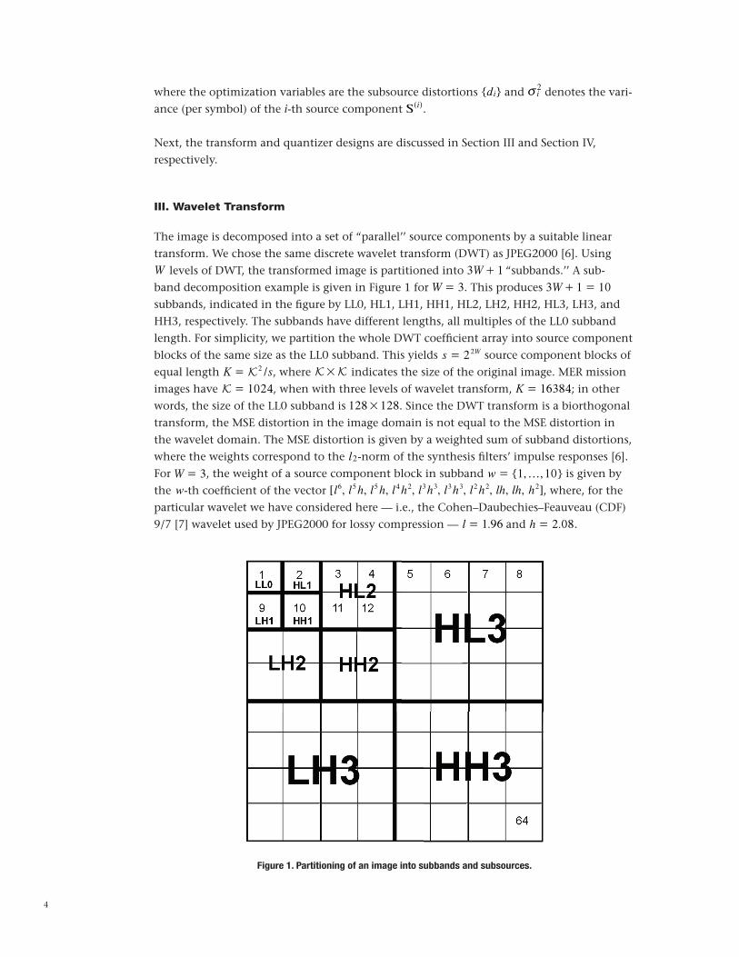
The image is decomposed into a set of “parallel’’ source components by a suitable linear transform. We chose the same discrete wavelet transform (DWT) as JPEG2000 [6]. Using W levels of DWT, the transformed image is partitioned into 3W+ 1 “subbands.’’ A sub-band decomposition example is given in Figure 1 for W = 3. This produces 3W+ 1 = 10 subbands, indicated in the figure by LL0, HL1, LH1, HH1, HL2, LH2, HH2, HL3, LH3, and HH3, respectively. The subbands have different lengths, all multiples of the LL0 subband length. For simplicity, we partition the whole DWT coefficient array into source component blocks of the same size as the LL0 subband. This yields s = 22W source component blocks of equal length K = K 2/s, where K #K indicates the size of the original image. MER mission images have K = 1024, when with three levels of wavelet transform, K = 16384; in other words, the size of the LL0 subband is 128 # 128. Since the DWT transform is a biorthogonal transform, the MSE distortion in the image domain is not equal to the MSE distortion in the wavelet domain. The MSE distortion is given by a weighted sum of subband distortions, where the weights correspond to the l2-norm of the synthesis filters’ impulse responses [6]. For W = 3, the weight of a source component block in subband w = {1,f,10} is given by the w-th coefficient of the vector [l6, l5h, l5h, l4h2, l3h3, l3h3, l2h2, lh, lh, h2], where, for the particular wavelet we have considered here — i.e., the Cohen–Daubechies–Feauveau (CDF) 9/7 [7] wavelet used by JPEG2000 for lossy compression — l = 1.96 and h = 2.08.

Figure 1. Partitioning of an image into subbands and subsources.

5

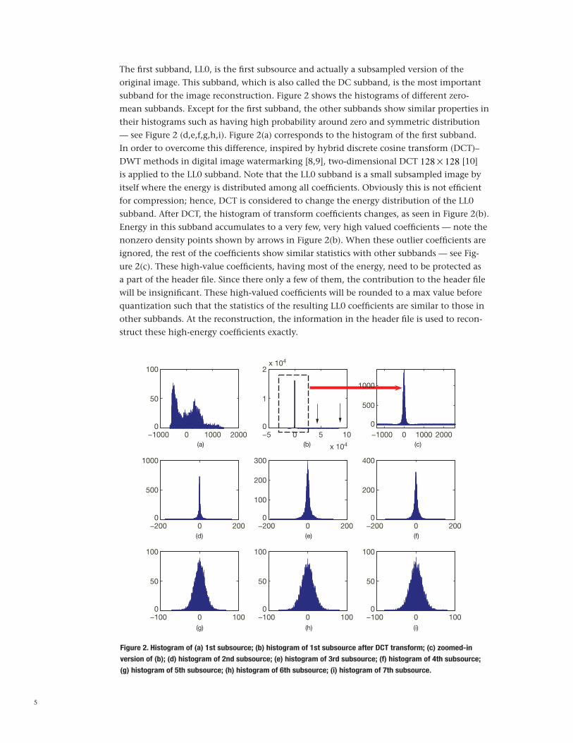
The first subband, LL0, is the first subsource and actually a subsampled version of the original image. This subband, which is also called the DC subband, is the most important subband for the image reconstruction. Figure 2 shows the histograms of different zero-mean subbands. Except for the first subband, the other subbands show similar properties in their histograms such as having high probability around zero and symmetric distribution — see Figure 2 (d,e,f,g,h,i). Figure 2(a) corresponds to the histogram of the first subband. In order to overcome this difference, inspired by hybrid discrete cosine transform (DCT)–DWT methods in digital image watermarking [8,9], two-dimensional DCT 128 # 128 [10] is applied to the LL0 subband. Note that the LL0 subband is a small subsampled image by itself where the energy is distributed among all coefficients. Obviously this is not efficient for compression; hence, DCT is considered to change the energy distribution of the LL0 subband. After DCT, the histogram of transform coefficients changes, as seen in Figure 2(b). Energy in this subband accumulates to a very few, very high valued coefficients — note the nonzero density points shown by arrows in Figure 2(b). When these outlier coefficients are ignored, the rest of the coefficients show similar statistics with other subbands — see Fig-ure 2(c). These high-value coefficients, having most of the energy, need to be protected as a part of the header file. Since there only a few of them, the contribution to the header file will be insignificant. These high-valued coefficients will be rounded to a max value before quantization such that the statistics of the resulting LL0 coefficients are similar to those in other subbands. At the reconstruction, the information in the header file is used to recon-struct these high-energy coefficients exactly.

Figure 2. Histogram of (a) 1st subsource; (b) histogram of 1st subsource after DCT transform; (c) zoomed-in

version of (b); (d) histogram of 2nd subsource; (e) histogram of 3rd subsource; (f) histogram of 4th subsource;

(g) histogram of 5th subsource; (h) histogram of 6th subsource; (i) histogram of 7th subsource.

−1000 0 1000 20000

50

100

a−5 0 5 100

1

2x 104

x 104b−1000 0 1000 20000

500

c

−200 0 2000

500

1000

d−200 0 200

0

100

200

300

e−200 0 200

0

200

400

f

−100 0 1000

50

100

g−100 0 100

0

50

100

h−100 0 100

0

50

100

j

1000

(b) (c)

(d) (e) (f)

(g) (h) (i)

(a)

6

Instead of using DCT on the LL0 subband, an extra level of DWT might be used for better compression characteristics at the expense of lowered block-length; i.e., smaller K value, which can affect the performance of modern block codes. Differential coding of the coeffi-cients is not considered due to possible error propagation.

Next, the quantizer selection for subsources is explained in Section IV.

IV. Quantizer

The simplest form of quantization employed by JPEG2000 is a dead-zone uniform scalar quantizer. A quantizer is called dead-zone if the center cell width is different than the other cells. The quantizer illustrated in Figure 3 is the quantizer used in JPEG 2000 Part I, where the dead-zone cell’s width is twice that of the other cells for any resolution level. In Fig-ure 3, an embedded dead-zone quantizer is shown for three different resolution levels.

p = 3

2 x

2 x

2 x

p = 2

p = 10

Quantizer Thresholds

Quantizer Reconstruction Points

–2 1

1 1

2 1– 1 1

3

2 2 2 2 2 2

3 3 3 3 3 3 3

2

= 2 x 2 x= 2 x1 32

1

3 3 3 3 3 3 3

Figure 3. An embedded dead-zone quantizer with p = 1,2,3.

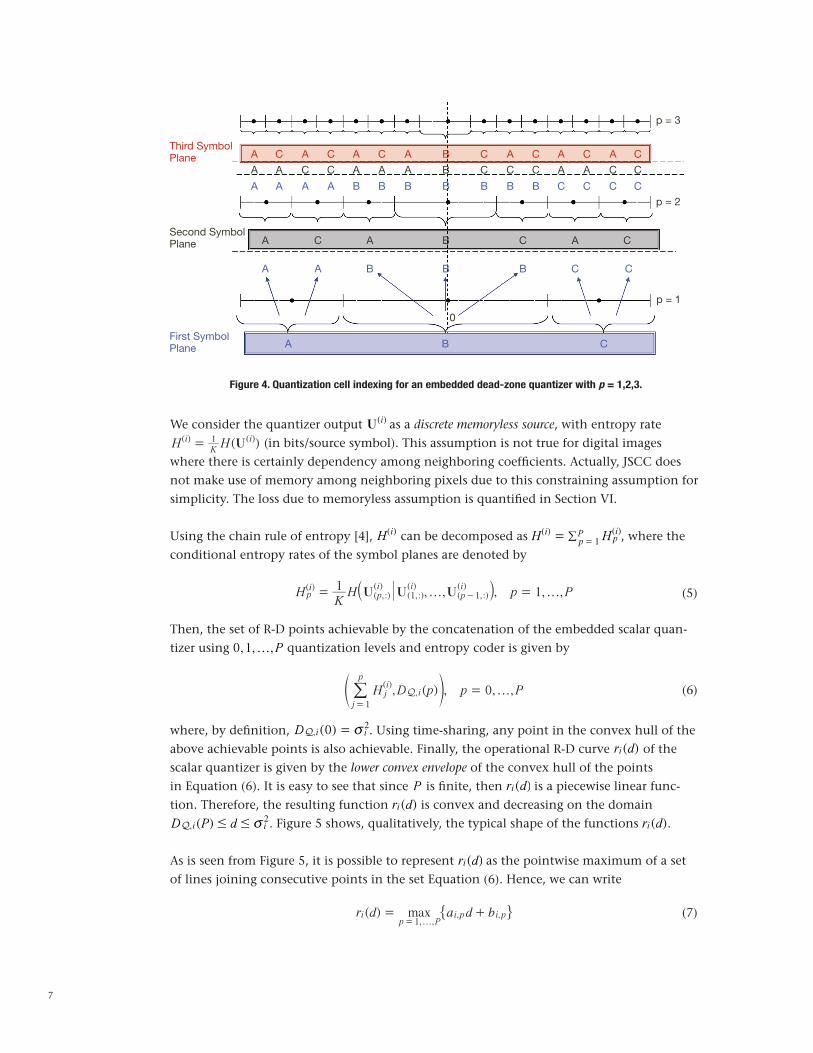
Notice that with dead-zone quantizers, the number of cells at any level p is given by 2 p+1 - 1. The cell regions are named by three symbols, {A,B,C}, as shown in Figure 4. As seen from Figure 4, quantization indices are described using multiple, consecutive symbol planes.

We denote the quantization function as Q : R " {A,B,C} P , where 2P+1 - 1 is the number of quantization regions for the highest level of refinement. The quantization distortion for the i-th source component is denoted by DQ,i (p) at a quantization level of p.

Let U(i) = Q (S(i)) denote the sequence of ternary quantization indices formatted as a P # K binary array. The p-th row of U(i), denoted by U(p,:)

(i) , is referred to as the p-th “sym-bol plane.’’ Without loss of generality, we let U(1,:)

(i) denote the first symbol plane, and U(2,:)(i),f,U(P,:)

(i) denote the other symbol planes with decreasing order of significance.

7

p = 3

p = 2

p = 1

Third SymbolPlane

Second SymbolPlane

First SymbolPlane

A

A

A

A

A

A B C

C

A

A

B

0

B

B

C

B

A

C

C

C

A

C

A

A

C

B

A

A

B

A

A

C

A

A

B

A

C

C

B

B

B

C

A

A

C

C

B

C

C

A

C

C

B

C

A

B

C

A

C

C

C

C

Figure 4. Quantization cell indexing for an embedded dead-zone quantizer with p = 1,2,3.

We consider the quantizer output U(i) as a discrete memoryless source, with entropy rate

( )H H U( ) ( )iK

i1= (in bits/source symbol). This assumption is not true for digital images where there is certainly dependency among neighboring coefficients. Actually, JSCC does not make use of memory among neighboring pixels due to this constraining assumption for simplicity. The loss due to memoryless assumption is quantified in Section VI.

Using the chain rule of entropy [4], H(i) can be decomposed as H(i) = Hp(i)

p= 1P/ , where the

conditional entropy rates of the symbol planes are denoted by

, , , 1, ,HKH p PU U U1( )

( ,:)( )

( ,:)( )

( ,:)( )

pi

pi i

pi

1 1f f= =-a k

Then, the set of R-D points achievable by the concatenation of the embedded scalar quan-tizer using 0,1,f,P quantization levels and entropy coder is given by

, ( ) , 0, ,H D p p P( )

,Qji

j

p

i

1

f==

f p/

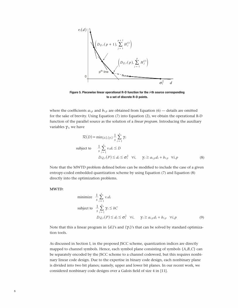
where, by definition, DQ,i (0) = vi2. Using time-sharing, any point in the convex hull of the above achievable points is also achievable. Finally, the operational R-D curve ri (d) of the scalar quantizer is given by the lower convex envelope of the convex hull of the points in Equation (6). It is easy to see that since P is finite, then ri (d) is a piecewise linear func-tion. Therefore, the resulting function ri (d) is convex and decreasing on the domain

DQ,i (P) # d # vi2. Figure 5 shows, qualitatively, the typical shape of the functions ri (d).

As is seen from Figure 5, it is possible to represent ri (d) as the pointwise maximum of a set of lines joining consecutive points in the set Equation (6). Hence, we can write

( ) maxr d a d b, ,

, ,ip P

i p i p1

= +f=" ,

(5)

(6)

(7)

8

Figure 5. Piecewise linear operational R-D function for the i-th source corresponding

to a set of discrete R-D points.

0

pth line

ri d^ h

DQ , i p + 1^ h, H j(i)

j = 1

p + 1

/f p

DQ , i p^ h, H j(i)

j = 1

p

/f p

vi2 d

where the coefficients ai,p and bi,p are obtained from Equation (6) — details are omitted for the sake of brevity. Using Equation (7) into Equation (2), we obtain the operational R-D function of the parallel source as the solution of a linear program. Introducing the auxiliary variables ci, we have

, ,

R minDs

sv d D

D P d i a d b i p

1

1subject to

,

, , ,Q

d i

i

s

i i

i

s

i i i i i p i i p

1

1

2

i i

6 6

#

# # $

c

v c

=

+

c=

=

^

^

h

h

" ", , /

/

Note that the MWTD problem defined before can be modified to include the case of a given entropy-coded embedded quantization scheme by using Equation (7) and Equation (8) directly into the optimization problems.

MWTD:

, ,

sv d

s

D

bC

P d i a d b i p

1

1

minimize

subject to

, , ,Q

i i

i

s

i

i

s

i i i i p i i pi

1

1

2 6 6

#

# # $

c

v c +

=

=

^ h

/

/

Note that this a linear program in {di}’s and {ci}’s that can be solved by standard optimiza-tion tools.

As discussed in Section I, in the proposed JSCC scheme, quantization indices are directly mapped to channel symbols. Hence, each symbol plane consisting of symbols {A,B,C} can be separately encoded by the JSCC scheme to a channel codeword, but this requires nonbi-nary linear code design. Due to the expertise in binary code design, each nonbinary plane is divided into two bit planes; namely, upper and lower bit planes. In our recent work, we considered nonbinary code designs over a Galois field of size 4 in [11].

(8)

(9)

9

(10)

(11)

Let Hp(i,u) be the conditional entropy of the upper bit plane of the ith symbol plane given previous symbol planes, and let Hp(i,l) denote the conditional entropy of the lower bit plane given previous symbol planes and also the upper bit plane of the ith symbol plane. Then,

H H H( ) ( , ) ( , )pi

pi u

pi l= +

For a given embedded scalar quantizer, we let ri denote the number of symbol planesof source component i that must be decoded according to the solution of the MWTD optimization problem. In the case of a separate design, if the output of the entropy coder is encoded with ideal channel codes, b will be given as follows:

bC

H H( , ) ( , )pi u

pi l

pi

s

11

i

=+r

==

//

In Section V, after discussing the details of the linear coding scheme, an expression for b is derived for the JSCC scheme. Then, comparing these two equations, we will be able to define the analogous MWTD problem for the JSCC case.

V. Linear Index Coding

Conventional fixed-to-variable-length entropy coding, such as Huffman or arithmetic cod-ing [4], is catastrophically nonrobust to residual channel errors.2 In practice, some robust-ness to mismatch in the channel parameter is desirable.

In order to cope with the mismatched case, several techniques have been proposed to heal the catastrophic effect of entropy coders. For example, a vast literature has dealt with the issue of making entropy coding “robust’’ to channel errors (see [12,13,14] and references therein). A simple approach along this line consists of partitioning the source block into shorter subblocks, and entropy coding each subblock separately. In this way, if a subblock contains a residual erasure, it is discarded and the missing block is somehow “concealed’’ in the source reconstruction. Broadly speaking, such an approach is adopted in the “error resilience’’ tools of JPEG2000 [15,16]. Similarly, ICER, a state-of-the-art image compressor employed by the JPL MER mission, divides an image into segments, as summarized in Sec-tion X; more details can be found in [1]. In order to cope with mismatch, we investigate the use of channel-optimized quantization [17,18], also known as “index coding’’ or “fixed-length index assignment.” The classical literature on channel optimized quantization has focused on ad hoc design and resulted in fixed-length indexing with no particular structure.3 Be-cause of complexity, this approach is limited to short block-lengths. More recently [3,19], linear coding is proposed in order to efficiently implement fixed-length index assignment. In this way, each quantizer bit plane is directly linearly encoded into a channel codeword. The resulting scheme provides naturally a channel-optimized successive refinement quantization scheme, and therefore it is ideally suited to the problems considered here.

2 See [3] for a detailed analysis of the effect of residual channel decoding errors on the end-to-end distortion for quantiza-tion followed by arithmetic coding.3 The channel-optimized codebook and its indexing are given through an exhaustive enumeration of the codewords.

10

(13)

(14)

(12)

A. Linear Bit-Plane Encoding and Multistage Decoding

We encode each of the 2ri bit planes for a single symbol plane separately using the linear coding. The upper bit plane U(p,:)

(i,u), for p # ri , are mapped into codewords X(p,:)(i,u)= U(p,:)

(i,u)G p,i,u

where G p,i,u denotes the K # np,i,u generator matrix of a suitable linear code and similar mapping is also applied to lower bit planes. This linear code is actually obtained by using a linear, systematic channel code. More details on this can be found in [3].

The coding rate K/np,i,u is chosen such that

/(1 )KH n C( , ), , , ,p

i up i u p i ui= +

where i p , i,u denotes the coding “overhead’’ for the p-th bit plane of the i-th source. The overhead definition is analogous to the overhead defined for channel coding in [20]. For the time being, we consider the coefficients i p , i,u to be given and greater than zero. They measure the suboptimality of the code with respect to ideal performance, which is K/np,i,u = Hp

(i,u) /C. In general, the coding rate overhead at each bit plane must be allocated such that each stage of the multistage BP decoder works with enough reliability in order to 1) provide reliable hard decisions in order to avoid error propagation in the multistage decoder; and 2) achieve output distortion close enough to the designed quantization distor-tion. Their calculation is discussed in Section VII.

The overall channel-encoded block is formed by the concatenation of all codewords {X(p,:)(i,u)}

and {X(p,:)(i,l)} for p = 1,f,P and i = 1,f,s , where it is understood that if some bit plane is

encoded with zero bits, the corresponding codeword is not present. The total source-chan-nel encoder output length is given by

N n n, , , ,p i u p i l

pi

s

11

i

= +r

==

//

Then,

(1 ) (1 )b

C

H H( , ), ,

( , ), ,p

i up i u p

i lp i l

pi

s

11

i i i=

+ + +r

==

//

Note that the value of b in the case of the proposed JSCC scheme in Equation (14) is equal to the value of b in the case of a separate scheme with an ideal channel code, and operational R-D curve pairs given by (1 ) (1 ), ( )H H D p

( , ), ,

( , ), , ,Qj

i up j u j

i lp j l ij

p1

i i+ + +=

a k/ using Equation (11). Then it follows that the MWTD problem defined in Section II for a separate scheme with ideal channel code and modified operational rate-distortion curves is formally identical to the MWTD problem that can be defined for the JSCC scheme.

In Section VI, the MWTD problem setup is first used to determine the pure compres-sion performance of the JSCC scheme. Then, in Section X, we provide results with noisy channels.

B. Multistage Decoding

As discussed earlier, the bit planes are encoded separately. On the other hand, the decoding of bit planes is done sequentially using previously decoded planes. Hence, this is a multi-

,

11

(15)

stage decoder. For example, in order to decode the (p, i,u)-th bit plane, the decoder must use the conditional a priori probability P(U(p,:)

(i)U(1,:)(i),f,U(p-1,:)

(i)) of the p-th symbol

plane, given the realization of the symbol planes 1,f,p- 1. Note that for the (p, i, l)-th bit plane, conditioning will be also done given the (p, i,u) bit plane. For simplicity, below we consider only the upper bit plane. This probability mass function (pmf) determines the conditional entropy Hp(i,u) in Equation (5) and collects the a priori information needed by the (p, i,u)-th decoder in order to decode the corresponding plane symbols. Letting Y(p,:)

(i,u) denote the channel output received corresponding to the transmission of X(p,:)

(i,u), a multistage decoder based on the maximum a posteriori probability (MAP) principle decodes the bit planes in sequence, according to the rule

, ,, ,Parg maxU uG U UY( ,:)( , )

{ }, ( ,:)

( )( ,:)( )

0,1( ,:( )

pi u

p ii

pi

pi

11K

ff= -!u

a kX X X

for p = 1,f,ri . Each p-th decoding stage makes use of the hard decisions UX(1,:)(i) ,f,UX(p-1,:)(i)

made at previous stages 1,f,p- 1 [21]. For modern sparse-graph codes, the MAP rule Equa-tion (15) would be computationally too complex. Instead, the low-complexity iterative BP algorithm is used at each stage of the multistage decoder [22]. The multistage BP decoder needs the knowledge of the conditional bit plane pmfs for each source component. For digital images, this must be estimated from the sequence of quantized DWT coefficients. In conventional source coding schemes (e.g., JPEG2000), these probabilities are implicitlyestimated by using sequential probability estimators [23] implemented together with the bit plane context model and arithmetic coding. For the a priori information calculation, we basically count symbols.

VI. Pure Compression

Lossless data compression (or “entropy coding’’) of general discrete sources can be achieved by linear coding [24,19]. This, combined with the well-known fact that linear coding achieves the capacity of symmetric channels [25], suggests a channel-optimized quantiza-tion scheme [17,18] based on linear coding of the quantization indices [19]. As discussed in [3], the proposed JSCC scheme can approach the Shannon separation limit H/C for send-ing a discrete memoryless source with entropy H over a symmetric channel with capacity C . Then, for the case of the pure compression scenario, the limiting performance of the proposed scheme can be found by setting C = 1 and i p , i,u = i p , i, l = 0 6p, i in the MWTD optimization problem, as described in Equation (9).

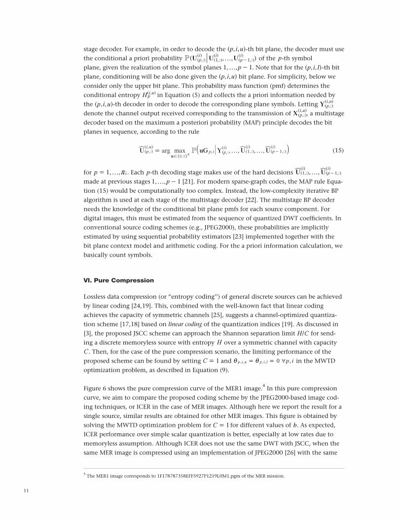
Figure 6 shows the pure compression curve of the MER1 image.4 In this pure compression curve, we aim to compare the proposed coding scheme by the JPEG2000-based image cod-ing techniques, or ICER in the case of MER images. Although here we report the result for a single source, similar results are obtained for other MER images. This figure is obtained by solving the MWTD optimization problem for C = 1 for different values of b. As expected, ICER performance over simple scalar quantization is better, especially at low rates due to memoryless assumption. Although ICER does not use the same DWT with JSCC, when the same MER image is compressed using an implementation of JPEG2000 [26] with the same

4 The MER1 image corresponds to 1F178787358EFF5927P1219L0M1.pgm of the MER mission.

12

Figure 6. Comparison of the JSCC scheme with DCT or without DCT of LL0 subband with respect to ICER.

MER1

With DCTICERWithout DCT

50

45

40

35

30

25

20

0 0.1 0.2 0.3 0.4 0.5 0.6 0.7 0.8 0.9 1bpp

PS

NR

DWT as JSCC, a very similar pure compression curve with respect to that of ICER is ob-tained. Hence, we explain the gap by the fact that the scalar quantization approach treats the transform coefficients in each source component block as being independently and identically distributed (i.i.d.), while ICER exploits the residual memory among the DWT coefficients thanks to its context mechanism, which accurately models the residual memory in the sequence of quantized DWT coefficients [1].

VII. Channel Code

As discussed in [3], the linear encoding of a bit plane is done using a systematic linear channel code encoder. Assume that for a block-length of K bits, K+ n channel symbols are created. Then the rate of this code is rc = K/ (K+ n). For a bit plane with entropy H over a channel with capacity C , the overhead i is related to rc using Equation (16):

HCr1 1 1c

i = - -c m

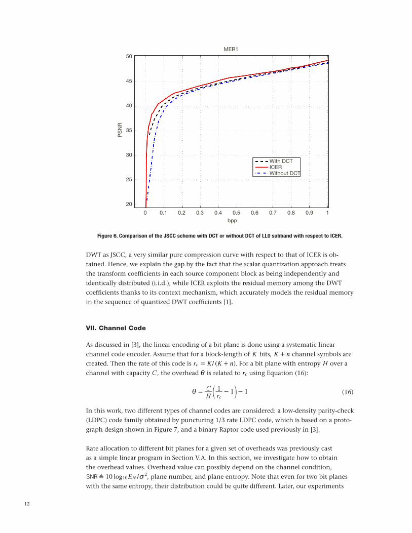
In this work, two different types of channel codes are considered: a low-density parity-check (LDPC) code family obtained by puncturing 1/3 rate LDPC code, which is based on a proto-graph design shown in Figure 7, and a binary Raptor code used previously in [3].

Rate allocation to different bit planes for a given set of overheads was previously cast as a simple linear program in Section V.A. In this section, we investigate how to obtain the overhead values. Overhead value can possibly depend on the channel condition,

SNR _ 10 log10EN /v2, plane number, and plane entropy. Note that even for two bit planes with the same entropy, their distribution could be quite different. Later, our experiments

(16)

13

Figure 7. By puncturing, we can obtain the following set of rates: 16/i 6i ! {17, 18,f, 47, 48}.

will show that bit planes with the same entropy have the same overhead value for a given channel condition. This observation provides a universal decision rule for overheads. Without this observation, JSCC would need to determine overhead for every possible plane distribution, which is obviously not feasible.

First, without making use of the above observation, for a single image the overhead values are obtained by both Monte Carlo simulations and extrinsic information transfer (EXIT) chart analysis (described in more detail next) for every bit plane. Using Equation (16), we can see that for a given channel and bit plane, there is a one-to-one relationship between i value and chosen code rate value. Hence, in the following we pose the problem as finding the right code rate value for each bit plane for a given channel condition. Similar to the i definition in Section V.A, the right code rate for the bit plane is the code rate at which the BER of the bit block is small enough to avoid error propagation and to avoid large diver-gence from quantization distortion values.

For a fixed channel condition, the highest rate code satisfying small enough error prob-ability for the chosen bit plane is selected as the corresponding code rate. We have found these code rates for different bit planes both in infinite case and finite case using EXIT chart analysis and Monte Carlo simulations, respectively.

Next, we explain how we have run EXIT charts for the JSCC scheme based on protograph code design and compare the finite and infinite block-length performances in Section VIII. In Section X, we explain in detail the binary Raptor code design we selected.

47 31151531

46 30141430

45 29131329

44 28121228

43 27111127

42 26101026

41 259925

40 248824

39 237723

38 226622

37 215521

36 204420

35 193319

34 182218

33 171117

32 0016

16

= =

14

VIII. Protograph-Based LDPC Codes

A. Infinite-Length Case: EXIT Chart Analysis

It has been shown in [3] that there exists a one-to-one mapping of the messages of the BP decoder for the JSCC problem and the messages of the BP decoder for a two-channel prob-lem as described in [3]. This means that the source-channel BP decoding can be analyzed, for example, by using the EXIT chart method, by considering the associated “virtual’’ chan-nel, where the all-zero codeword from the associated systematic code is transmitted partly on a binary additive noise channel with noise realization identical to the source realization of the source-channel problem and partly on the AWGN channel.

The standard analysis tool for graph-based codes under BP iterative decoding, in the limit of infinite block-length, is density evolution (DE) [27,28]. DE is typically computationally heavy, and numerically not very well conditioned. A much simpler approximation of DE consists of the so-called EXIT chart, which corresponds to DE by imposing the restriction that message densities are of some particular form. In particular, the EXIT with Gaussian approximation (GA) assumes that at every iteration the BP message distribution is Gauss-ian having a particular symmetry condition, which imposes that the variance is equal to 2 times the mean [29]. At this point, densities are uniquely identified by a single parameter, and the approximate DE tracks the evolution of this single parameter across the decoding rounds.

In particular, the EXIT chart tracks the mutual information between the message on a random edge of the graph and the associated binary variable node connected to the edge. By the isomorphism proved in [3], the JSCC scheme and the “two-channel’’ scheme have identical BER performance. For the sake of completeness, in this section we apply the EXIT chart analysis to the “two-channel’’ case. The resulting EXIT chart applies directly to the JSCC EXIT chart for a binary source.

Let Nc denote the number of checknodes, while Nv denotes the number of variable nodes. Different than a random ensemble, a base protograph can have parallel edges between a parity and a checknode [30]. Let hij denote the number of parallel edges between the jth

variable and ith checknode. EXIT charts can be seen as a multidimensional dynamic system. We are interested in studying the fixed points and the trajectories of this system. As such, an EXIT chart on the base protograph has the following state variables:

Xij — Mutual information between a message sent along the (i ! j) edge (i.e., ith check, jth variable) and the jth variable node symbol.

Yij — Mutual information between a message sent along the (i " j) edge (i.e., ith check, jth variable) and the jth variable node symbol.

C j — Mutual information between the jth variable node and the corresponding log likelihood ratio (LLR) at the channel output (channel capacity of the jth variable node). Note that if a node is punctured, C j = 0.

We consider the class of EXIT functions that make use of Gaussian approximation of the BP messages. Imposing the symmetry condition and Gaussianity, the conditional distribution

15

(17)

(18)

(19)

(20)

of each message L in the direction from a variable to checknode is Gaussian +N(n,2n) for some value n ! R+ . Hence, letting V denote the corresponding bit node variable, we have

; 1 1EL logI V e JL2 _ n= - + -^ ^ ^h h h6 @

where L +N(n,2n).

In BP, the message on edge (i ! j) is the sum of all messages incoming to i on all other edges. The sum of Gaussian random variables is also Gaussian, and its mean is the sum of the means of the incoming messages. As far as checknodes are concerned, we use the well-known quasi-duality approximation and replace checknodes with bit nodes by changing mutual information into entropy (i.e., replacing x by 1 - x). Then iterative equations are as follows:

Y

X X1 1 1

X

Y

YJ J

J

J J C

J J1

11 1 1

1 1

ij sj sj ij

s i

ij j

ij is is ij ij

s j

h

h h

h=

= - -

+ - +

- + -

!

!

- - -

- -

^ ^ ^ ^c

^ ^ ^c

h h h hm

h h hm

/

/

Decision step:

jYJ

P Q

J C

2

1 1j sj

s

sj

jj

n h

n

=

=

+- -^ ^

c

h h

m

/

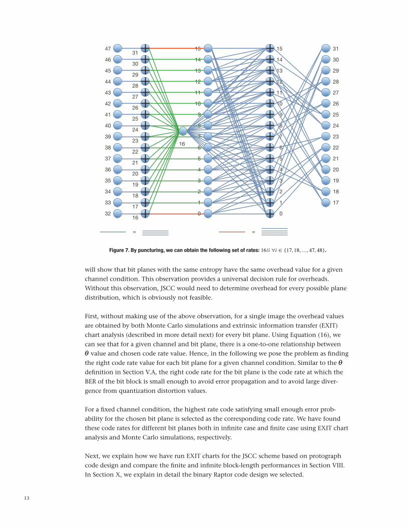
Figure 8 shows the notation used to describe the protograph.

Figure 8. Notation used to describe the protograph.

j iX

Y

B. EXIT Charts for Two-Channel Model

For variable nodes that are systematic, the channel is not stationary. As explained in [3], the systematic nodes correspond to virtual channels, which can be described by the source model.

16

(21)

(22)

(23)

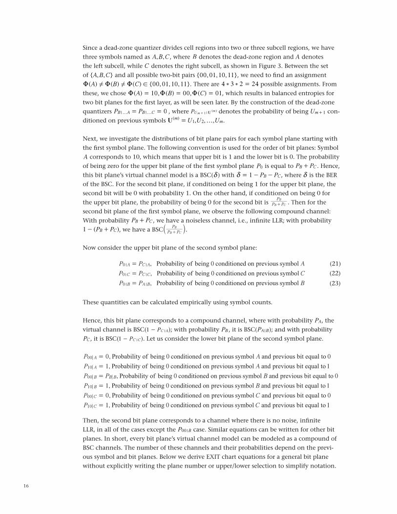
Since a dead-zone quantizer divides cell regions into two or three subcell regions, we have three symbols named as A,B,C , where B denotes the dead-zone region and A denotes the left subcell, while C denotes the right subcell, as shown in Figure 3. Between the set of {A,B,C} and all possible two-bit pairs {00,01,10,11}, we need to find an assignment U(A) ! U(B) ! U(C) ! {00,01,10,11}. There are 4 ) 3 ) 2 = 24 possible assignments. From these, we chose U(A) = 10,U(B) = 00,U(C) = 01, which results in balanced entropies for two bit planes for the first layer, as will be seen later. By the construction of the dead-zone quantizers PB |fA = PB |fC = 0 , where PUm+ 1 |U (m ) denotes the probability of being Um+1 con-ditioned on previous symbols U(m) = U1,U2,f,Um.

Next, we investigate the distributions of bit plane pairs for each symbol plane starting with the first symbol plane. The following convention is used for the order of bit planes: Symbol

A corresponds to 10, which means that upper bit is 1 and the lower bit is 0. The probability of being zero for the upper bit plane of the first symbol plane P0 is equal to PB+ PC . Hence, this bit plane’s virtual channel model is a BSC(d) with d = 1- PB- PC, where d is the BER of the BSC. For the second bit plane, if conditioned on being 1 for the upper bit plane, the second bit will be 0 with probability 1. On the other hand, if conditioned on being 0 for the upper bit plane, the probability of being 0 for the second bit is P P

P

B C

B

+ . Then for the second bit plane of the first symbol plane, we observe the following compound channel: With probability PB+ PC , we have a noiseless channel, i.e., infinite LLR; with probability 1 - (PB+ PC), we have a BSC P P

P

B C

B

+a k.

Now consider the upper bit plane of the second symbol plane:

, 0

, 0

, 0

P P A

P P

P P

C

B

Probability of being conditioned on previous symbolProbability of being conditioned on previous symbolProbability of being conditioned on previous symbol

| |

| |

| |

A C A

CC C

B A B

0

0

0

=

=

=

These quantities can be calculated empirically using symbol counts.

Hence, this bit plane corresponds to a compound channel, where with probability PA, the virtual channel is BSC(1 - PC | A); with probability PB , it is BSC(PA |B); and with probability

PC , it is BSC(1 - PC | C). Let us consider the lower bit plane of the second symbol plane.

0, 0 0

,

,

,

,

,

P A

P A

P P B

P B

P C

P C

1 0 1

0 0

1 0 1

0 0 0

1 0 1

Probability of being conditioned on previous symbol and previous bit equal toProbability of being conditioned on previous symbol and previous bit equal toProbability of being conditioned on previous symbol and previous bit equal to

Probability of being conditioned on previous symbol and previous bit equal toProbability of being conditioned on previous symbol and previous bit equal toProbability of being conditioned on previous symbol and previous bit equal to

00

10

00

10

00

10

A

A

B B B

B

C

C

=

=

=

=

=

=

Then, the second bit plane corresponds to a channel where there is no noise, infinite LLR, in all of the cases except the P00 |B case. Similar equations can be written for other bit planes. In short, every bit plane’s virtual channel model can be modeled as a compound of BSC channels. The number of these channels and their probabilities depend on the previ-ous symbol and bit planes. Below we derive EXIT chart equations for a general bit plane without explicitly writing the plane number or upper/lower selection to simplify notation.

17

(24)

(25)

(26)

Let M denote the maximum number of BSC channels that a bit plane’s virtual compound channel can be modeled with. Then, for a variable node j , let C j

(c), c ! {1,f,M} denote dif-

ferent possible capacity values with probabilities e j(c).

Note that for nonsystematic nodes, although we have a single, common capacity value, we can set C j = C j

(1)=f = C j

(M) and e j(c)= 1/M . Hence, every variable node has M possible

channel capacities.

Note that due to the structure of the JSCC problem, all of the nonsystematic nodes have the same channel capacity value. Similarly, all of the systematic nodes have the same chan-nel capacity and probability values from the viewpoint of EXIT chart calculations.

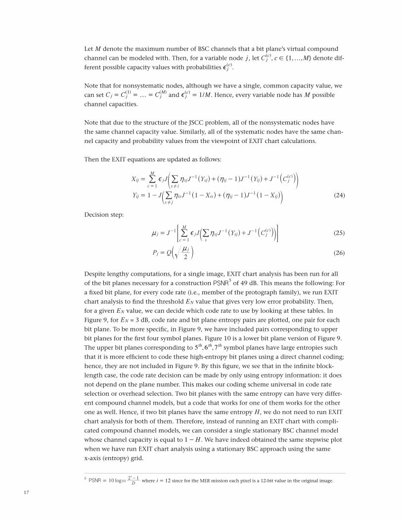
Then the EXIT equations are updated as follows:

X J J Y

Y J J X

J Y J C

J X1 1

1

1 1

1 1 1

1 1

( )ij j

c

M

sj

s i

sj ij ij

ij is

s j

is ij ij

jc

1

e h

h

h

h

=

= - -

+ - +

+ - -

!

!

=

- - -

- -

^ ^ ^ af

^ ^ ^c

h h h kp

h h hm

/ /

/

Decision step:

J J J Y J C

2

1 1 1 ( )j j sj sj

jj

c

M

sjc

1

n

n

e h= +- - -

=

P Q=

^ ac

c

h km

m

> H/ /

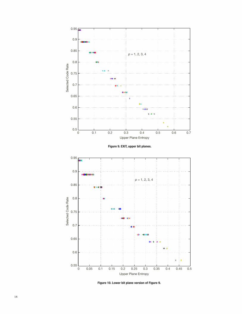
Despite lengthy computations, for a single image, EXIT chart analysis has been run for all of the bit planes necessary for a construction PSNR

5 of 49 dB. This means the following: For a fixed bit plane, for every code rate (i.e., member of the protograph family), we run EXIT chart analysis to find the threshold EN value that gives very low error probability. Then, for a given EN value, we can decide which code rate to use by looking at these tables. In Figure 9, for EN = 3 dB, code rate and bit plane entropy pairs are plotted, one pair for each bit plane. To be more specific, in Figure 9, we have included pairs corresponding to upper bit planes for the first four symbol planes. Figure 10 is a lower bit plane version of Figure 9. The upper bit planes corresponding to 5th,6th,7 th symbol planes have large entropies such that it is more efficient to code these high-entropy bit planes using a direct channel coding; hence, they are not included in Figure 9. By this figure, we see that in the infinite block-length case, the code rate decision can be made by only using entropy information: it does not depend on the plane number. This makes our coding scheme universal in code rate selection or overhead selection. Two bit planes with the same entropy can have very differ-ent compound channel models, but a code that works for one of them works for the other one as well. Hence, if two bit planes have the same entropy H , we do not need to run EXIT chart analysis for both of them. Therefore, instead of running an EXIT chart with compli-cated compound channel models, we can consider a single stationary BSC channel model whose channel capacity is equal to 1 -H . We have indeed obtained the same stepwise plot when we have run EXIT chart analysis using a stationary BSC approach using the same x-axis (entropy) grid.

5 PSNR log10D2 1i

10=-

where i = 12 since for the MER mission each pixel is a 12-bit value in the original image.

18

Figure 10. Lower bit plane version of Figure 9.

Figure 9. EXIT, upper bit planes.

p = 1, 2, 3, 4

0.95

0.9

0.85

0.8

0.75

0.7

0.65

0.6

0.55

0.50 0.1 0.2 0.3 0.4 0.5 0.6 0.7

Upper Plane Entropy

Sel

ecte

d C

ode

Rat

e

p = 1, 2, 3, 4

0.95

0.9

0.85

0.8

0.75

0.7

0.65

0.6

0.550 0.05 0.1 0.15 0.2 0.25 0.3 0.35 0.4 0.45 0.5

Upper Plane Entropy

Sel

ecte

d C

ode

Rat

e

19

C. Finite Length

For each p-th bit plane of the i-th source component, the overhead i p, i,u is optimized as follows: The multistage decoder is initialized by the perfect knowledge of the symbol planes from 1,f,p- 1. Then, a Monte Carlo simulation of the BP decoder is run with this information for coding block-length np, i,u = (1 + ip, i,u)KHp(i,u) /C , for increasing values of i p, i,u $ 0, which corresponds to decreasing values of code rates from the given LDPC code family. We stop increasing the overhead factor when the target p-th level distortion DQ,i (p) is reached and when the residual post-decoding erasure rate is sufficiently close to zero. The resulting value of i p, i,u yields the required overhead for the upper bit plane. Lower bit plane overhead can be obtained similarly. This optimization is performed off-line.

Obviously, this Monte Carlo simulation will become very costly if we need to do this for every bit plane configuration. Inspired by the staircase (universality) result of the EXIT chart analysis, we have run Monte Carlo simulations only for the stationary BSC model for a wide range of channel capacities. Then, by simulations, we have indeed verified that the code rates selected for the stationary BSC model also work for any compound channel model suggested by a specific bit plane as long as their capacity and entropy values match in the sense of C = 1-H .

IX. Binary Raptor Codes

Similar to the approach followed for protograph LDPC codes, we could run EXIT chart analysis or do finite-length simulations for every bit plane using their specific compound channel model. Instead, we worked with a stationary BSC model for a wide range of chan-nel capacities. Then we have verified that the code rates selected only according to the entropy using a stationary BSC model are also good codes for the corresponding bit plane with nonstationary distribution.

For this work, we used the Raptor codes used in [3]. To be specific, we considered Raptor codes with the “LT’’ degree distribution [31].

( ) 0.008 0.494 0.166 0073 0.083

0.056 0.037 0.056 0.025 0.003

x x x x x x

x x x x x

2 3 4 5

8 9 19 65 66

X = + + + +

+ + + + +

As outer code, we used a regular high-rate LDPC code with degrees (2,100) and rate 0.98.

EXIT chart analysis for the JSCC scheme using Raptor codes was first done in [3]. For the sake of completeness, we include the derivations of [3] below.

Finite-length performance using binary Raptor codes is obtained similar to Section VIII.B; hence, we directly provide simulation results in Section X for the finite-length case without any need for further explanation.

For the graph induced by the Raptor (LT) distribution, we define the input nodes (also called information bitnodes), the output nodes (also called coded bitnodes) and the check-

(27)

20

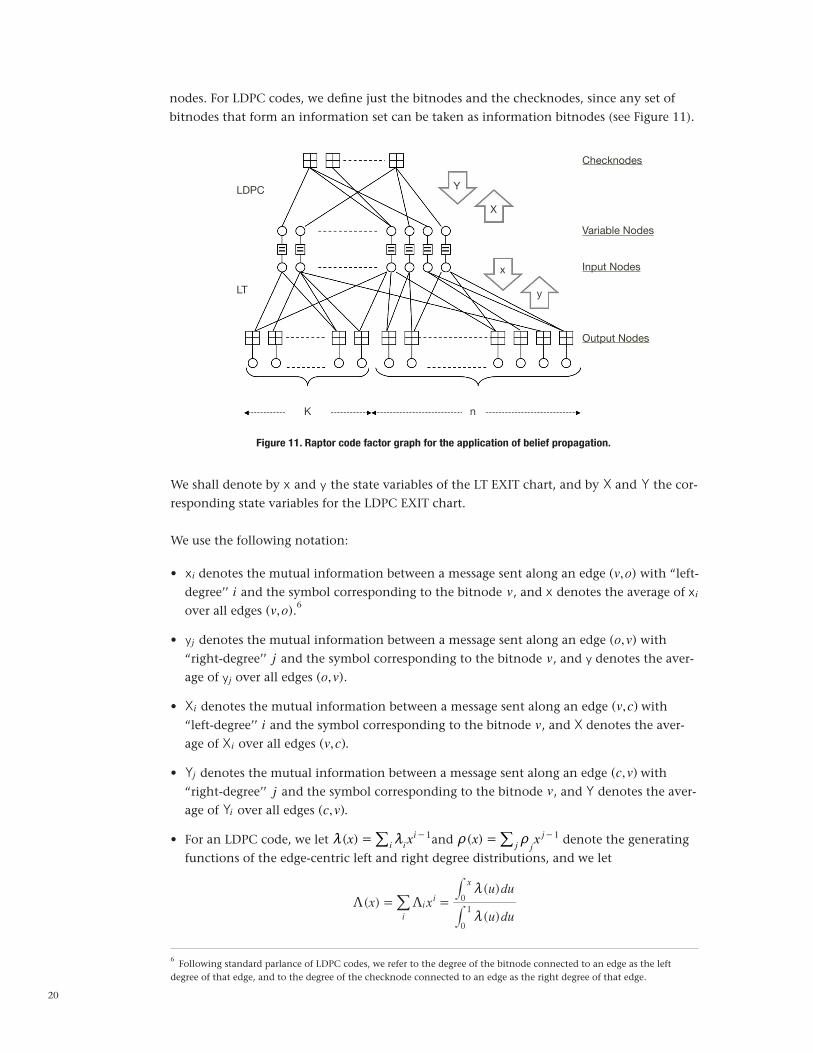
nodes. For LDPC codes, we define just the bitnodes and the checknodes, since any set of bitnodes that form an information set can be taken as information bitnodes (see Figure 11).

Figure 11. Raptor code factor graph for the application of belief propagation.

LDPC

LT

Checknodes

Variable Nodes

Input Nodes

Output Nodes

K n

Y

X

y

x

We shall denote by x and y the state variables of the LT EXIT chart, and by X and Y the cor-responding state variables for the LDPC EXIT chart.

We use the following notation:

• xi denotes the mutual information between a message sent along an edge (v,o) with “left-degree’’ i and the symbol corresponding to the bitnode v, and x denotes the average of xi over all edges (v,o).6

• yj denotes the mutual information between a message sent along an edge (o,v) with “right-degree’’ j and the symbol corresponding to the bitnode v, and y denotes the aver-age of yj over all edges (o,v).

• Xi denotes the mutual information between a message sent along an edge (v,c) with “left-degree’’ i and the symbol corresponding to the bitnode v, and X denotes the aver-age of Xi over all edges (v,c).

• Yj denotes the mutual information between a message sent along an edge (c,v) with “right-degree’’ j and the symbol corresponding to the bitnode v, and Y denotes the aver-age of Yi over all edges (c,v).

• For an LDPC code, we let m(x) = mi/

ixi-1and t (x) = t

j/

jx j-1 denote the generating

functions of the edge-centric left and right degree distributions, and we let

( )( )

( )x x

u du

u duii

i

x

0

1

0

m

mKK = =/

##

6 Following standard parlance of LDPC codes, we refer to the degree of the bitnode connected to an edge as the left degree of that edge, and to the degree of the checknode connected to an edge as the right degree of that edge.

21

denote the bit-centric left degree distribution.

• For an LT code, we let k(x) = ki/

ixi-1 denote the edge-centric degree distribution of the

input nodes, and we let ~ (x) = ~j/

jx j-1 denote the edge-centric degree distribution

of the “output nodes’’ or, equivalently, the edge-centric degree distribution of the checknodes. The node-centric degree distribution of the checknodes is given by

( )( )

( )x x

u du

u duj

i

j

x

0

1

0

~

~X X= =/

##

• For the concatenation of the LT code with the LDPC code, we also have the node-centric degree distribution of the LT input nodes. This is given by

( )( )

( )x x

u du

u duii

i

x

0

1

0% %k

k= =/

##

Similar to Section VIII.A, we make use of Gaussian assumption to derive

(( 1) ( ) ( ))x yJ i J J Ci1 1= - +- -

where C is the mutual information (capacity) between the bitnode variable and the cor-responding LLR at the (binary-input symmetric output) channel output. In the Raptor case, the bitnodes correspond to variables that are observed through a virtual channel by the LDPC decoder. Averaging with respect to the edge degree distribution, we have

x y(( 1) ( ) ( ))i J J CJii

1 1k= - +- -/

Then, using quasi-duality approximation for checknodes, we write

jy x1 (( 1) (1 ) (1 ))J j J J C1 1= - - - + -- -

Let us consider now the “two-channel” scenario induced by the JSCC isomorphism. Let

K denote the number of source bits, and n denote the number of parity bits. In the cor-responding LT code, we have K+ n output nodes. The first K output nodes are “observed’’ through a channel with capacity 1 -H (i.e., the channel corresponds to the source statis-tics), while the second n output nodes are observed through the actual transmission chan-nel, with capacity C .

This channel feature is taken into account by an outer expectation in the EXIT functions. Therefore, the LT EXIT chart can be written in terms of the state equations as following

x y

y Y

(( 1) ( ) ( ))

(( 1) ( ) ( ))

J i J J c

J i J kJ

k i k

ik

i

i

k

k

1 1

1 1k

k

K

K .= - +

= - +

- -

- -

//

//

where K/ (K+ n) = b and n/ (K+ n) = 1 - b, and

(28)

22

(30)

(31)

(29)

y x x1 (( 1) (1 ) ( )) (1 ) (( 1) (1 ) (1 ))J j J J H J j J J Cj

j

1 1 1 1~ b b= - - - + + - - - + -- - - -6 @/

where . ck is the mutual information input by the LDPC graph into the LT code graph via the node v of degrees (i,k) as explained in the following.

Equation (29) follows from the fact that a random edge (o,v) is connected with probability

b to a source bit (i.e., to the channel with capacity 1 -H ), while with probability 1 - b to a parity bit (i.e., to the channel with capacity C ).

Consider an LDPC bitnode v that coincides with an input node of the LT code. The degree of this node with respect to the LDPC graph is k, while the degree of v with respect to the LT graph is i. For a randomly generated graph, and a random choice of v, k and i are inde-pendent random variables, with joint distribution given by

,i k i k%P K=

The mutual information input by the LT graph into the LDPC graph via the node v of de-grees (i,k) is given by

y( ( ))c J iJi1

- = -

Therefore, the LDPC EXIT chart can be written in terms of the state equations

X Y

Y y

(( 1) ( ) ( ))

(( 1) ( ) ( ))

J k J J c

J k J iJ

k i i

ik

k i

ik

1 1

1 1

-%

%

m

m

= - +

= - +

- -

- -

//

//

and

Y X1 (( 1) (1 ))J J 1,t= - - -,

-,/

The mutual information input by the LDPC graph into the LT graph via the node v of de-grees (i,k) is given by

Y( ( ))c J kJk1

. = -

Equations (30), (31), (28), and (29) form the state equations of the global EXIT chart of the concatenated LT–LDPC graph, where the state variables are x,y,X,Y, while the parameters are H , C , and b, and the degree sequences ~ , k,t, and m .

Finally, in order to get the reconstruction distortion, we need to obtain the conditional probability density function (pdf) of the LLR’s output by BP for the source bits. Under the Gaussian approximation, the LLR is Gaussian. Let n j denote the mean of the LLR of a source bitnode corrected to a checknode of degree j , given by

x1 ( (1 )) ( )J J jJ J H1j1 1 1n = - - + -- - -^ h

23

(32)

Then, we approximate the average BER of the source bits as

P Q2

b jj

j

nX= c m/

X. Results

In this section, we present in some detail the deep-space image transmission scheme cur-rently employed by the MER mission. This scheme, which represents the benchmark for comparison to the JSCC scheme presented in this article, is based on a separated approach including ICER [1] and state-of-the-art channel codes for deep-space transmission.

ICER is a progressive, wavelet-based image data compressor based on the same principles as JPEG2000, including a DWT, quantization, segmentation, and entropy coding of the blocks of quantization indices with arithmetic coding and an adaptive probability model estimator based on context models. These blocks have differences with respect to their counterparts in JPEG2000 to handle properties of deep-space communication (details can be found in [1]).

ICER partitions an image into segments to increase robustness against channel errors. A segment “loosely’’ corresponds to a rectangular region of the image. Each image segment is compressed independently by ICER so that a decoding error due to data loss affecting one segment has no impact on decoding of the other segments. The encoded bits corresponding to all the segments are concatenated. The mapping of segments to variable-length packets (and to fixed-length frames) is handled outside of ICER according to the the Consulta-tive Committee for Space Data Systems (CCSDS) packet telemetry standard [1,32]. For the

PSNR values and number of segments we work with, a segment almost always corresponds to a single packet. Hence, in the following, we skip packetization but directly work with segments and frames.7 The encoded bits of segments are divided into fixed-length frames that are individually channel encoded with a fixed channel code rate Rc !Rc, where Rc denotes a finite set of possible coding rates. The channel coding rate is chosen according to the channel SNR . Rc can be chosen from a set of different code rates Rc according to chan-nel conditions.

A segment is generally divided into several frames. Data losses occur at the frame level. A whole segment is discarded even if a single frame corresponding to that segment is lost. When a frame loss occurs, it typically affects a single segment, but it could affect two seg-ments if the lost frame straddled the boundary between two segments. If a fixed PSNR value is targeted, the discarded segments must be retransmitted. Note that the delay and the cost of retransmission and feedback is significant when deep-space image transmission is consid-ered. In contrast, for the proposed JSCC we do not consider any retransmission.

In order to compare the performance of the proposed JSCC scheme with that of the base-line scheme, we consider an experiment where a target PSNR is fixed. For both schemes, the

7 A MER image is 1024 × 1024 pixels. This corresponds to 217 bytes at a compression ratio of 1 bpp in order to reach PSNR ∼ 49 dB. Packet length is 216 bytes. Then, for the PSNR values we are interested in, it’s almost always going to be a single packet per segment, provided that 2 or more segments are used for an image. We have used 32 segments for an image as it gave the best performance for the separated approach.

24

bandwidth expansion factor b for the fixed target PSNR depends on the particular imageand on the channel SNR . For a given set of test images, we compare the two schemes in terms of b versus SNR , for the fixed target PSNR.

As explained above, when a frame is lost, the whole segment is retransmitted. Frame-error rate (FER) is assumed to be fixed during the entire transmission process. Then the number of transmissions necessary for a segment is a geometric random variable with success probabil-ity depending only on the FER and the number of frames corresponding to the segment’s data, denoted by F . Therefore, the expected number of transmissions for a segment is given by

Z FER1F

= -^ h

The number of frames spanning each segment is not constant, in general, and some frame may straddle across two segments; hence, this analysis is not exact. Nevertheless, we can find tight upper and lower bounds to the average number of channel uses necessary to achieve the target PSNR, for given channel SNR and chosen coding rate Rc .

For a given SNR value, the baseline scheme chooses a code from standard JPL codes. For a well-matched SNR and rate pair, the FER is very low such that the expected number of re-transmissions is insignificant. Then b is very close to the “one-shot’’ transmission value; i.e., B/ (Rc), where B is the total number of ICER-encoded bits for the image at the given target

PSNR.

For a given code rate, as the SNR increases beyond the matched point, b will stay fixed, since retransmissions are getting more and more insignificant. On the other hand, when the SNR is lower than the matched point, the FER increases significantly and retransmis-sions become significant. In this case, b rapidly increases and becomes much larger than its minimum value B/ (Rc). If the SNR is very low with respect to a given channel code, then it might be more advantageous to switch to a lower-rate code.

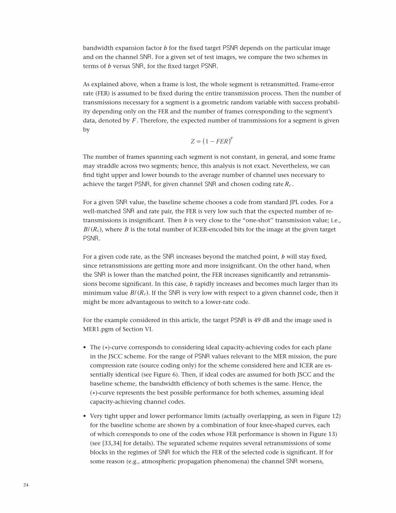
For the example considered in this article, the target PSNR is 49 dB and the image used is MER1.pgm of Section VI.

• The ())-curve corresponds to considering ideal capacity-achieving codes for each plane in the JSCC scheme. For the range of PSNR values relevant to the MER mission, the pure compression rate (source coding only) for the scheme considered here and ICER are es-sentially identical (see Figure 6). Then, if ideal codes are assumed for both JSCC and the baseline scheme, the bandwidth efficiency of both schemes is the same. Hence, the ())-curve represents the best possible performance for both schemes, assuming ideal capacity-achieving channel codes.

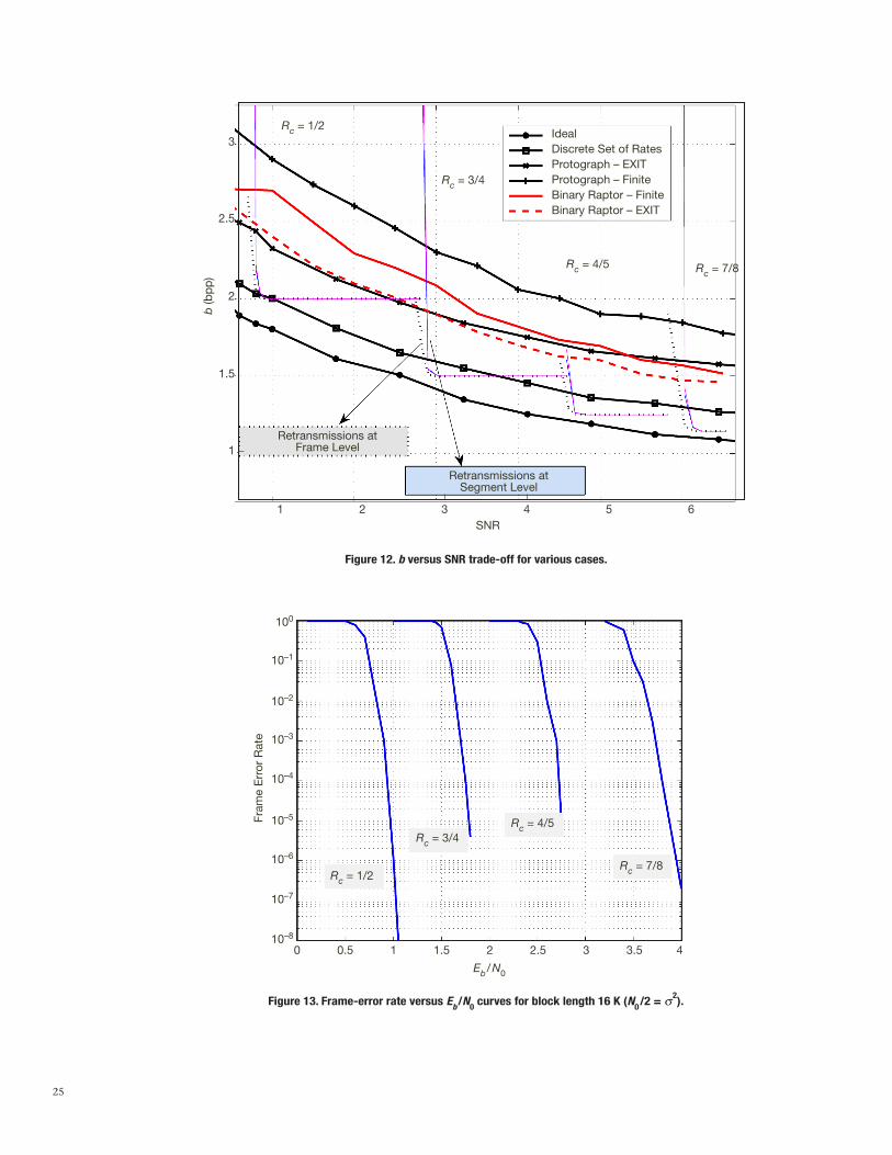
• Very tight upper and lower performance limits (actually overlapping, as seen in Figure 12) for the baseline scheme are shown by a combination of four knee-shaped curves, each of which corresponds to one of the codes whose FER performance is shown in Figure 13) (see [33,34] for details). The separated scheme requires several retransmissions of some blocks in the regimes of SNR for which the FER of the selected code is significant. If for some reason (e.g., atmospheric propagation phenomena) the channel SNR worsens,

25

Figure 13. Frame-error rate versus Eb /N0 curves for block length 16 K (N0 /2 = s 2).

Figure 12. b versus SNR trade-off for various cases.

SNR

Rc = 1/2

Rc = 3/4

Rc = 4/5 Rc = 7/8

1 2 3 4 5 6

3

2.5

2

1.5

1

IdealDiscrete Set of RatesProtograph – EXITProtograph – FiniteBinary Raptor – FiniteBinary Raptor – EXIT

Retransmissions at Segment Level

Retransmissions at Frame Level

b (b

pp

)

Rc = 1/2

Rc = 3/4Rc = 4/5

Rc = 7/8

100

10–1

10–2

10–3

10–4

10–5

10–6

10–7

10–8

0 0.5 1 1.5 2 2.5 3 3.5 4

Eb / N0

Fram

e E

rror

Rat

e

26

eventually the separated scheme must decrease the coding rate and jump to the next available lower-rate code. Hence, the baseline scheme’s performance is given as the lower envelope of these four curves indicated as “Retransmissions at Segment Level”; Rc value corresponding to each curve is also shown in Figure 12.

• Although an entire segment is retransmitted due to a single frame loss according to cur-rent deep-space image transmission standards [1,32], this is obviously very inefficient. A more efficient system would use ICER with retransmission at the frame level; in other words, sending only lost frames, not the entire segment. Again using the expectation of geometric random variable (with success rate 1 - FER for each frame), the average num-ber of transmissions can be exactly calculated. These curves are indicated as “Retransmis-sions at Frame Level’’ in Figure 12.

• The (#)-curve is the result of EXIT calculations for protograph LDPC codes, while the (+)-curve is the finite-length results of the same codes.

• The curve with is plotted assuming we have capacity-achieving codes but not at all rates in a continuous rate range (rather at discrete rate points given by the LDPC pro-tograph code family we use; hence, available rates are 16/17,...16/48). The difference between the )-curve and the -curve shows us how much we lose due to a discrete set of channel code rates.

• The (-)-curve is the result of EXIT calculations for binary Raptor codes when the LDPC code described in Section IX is used with the LT degree distribution in Equation (27). Shokrollahi reported this degree distribution in [20] to be used for erasure channels. The (--)-curve corresponds to finite-length simulations of the same degree distribution.

XI. Conclusions and Future Work

For finite block-length, the separated scheme requires several retransmissions of some blocks in the regimes of SNR for which the FER of selected code is non-negligible. If, for some reason (e.g., atmospheric propagation phenomena), the channel SNR worsens,eventually the separated scheme must decrease the coding rate and jump to the next avail-able lower-rate code.

From Figure 12, we observe that the performance of the JSCC scheme assuming capacity-achieving codes for a continuum of rate values ()-line) is very promising; i.e., the b value required for any channel condition is less than of the ICER and channel code concatena-tion. Besides, JSCC provides a smooth trade-off curve between b and channel SNR, unlike the “knee’’-shaped curves of the separated scheme.

On the other hand, currently the best finite-length performance of JSCC suffers from a sig-nificant penalty. As a consequence, the current JSCC design is not as efficient as the separat-ed approach for the presented numerical results, with a fixed target PSNR. Note that in this experiment, we only discuss b as the performance criteria. But one should remember that the separated scheme achieves the current curve with retransmissions and hence requires feedback and delay tolerance, which is not reflected in Figure 12.

27

As discussed earlier, the difference between the )-curve and the -curve shows us how much we lose due to a discrete set of LDPC channel code rates. Although the rate range of the LDPC code family can cover both the maximum and minimum entropy bit planes, the available rate grid is not fine enough to match each bit plane to a code rate with low over-head. This has been improved by using Raptor codes in which the rate region is continuous. The line corresponding to the performance of the binary Raptor codes for finite length is in-dicated in the figure. Compared with the finite-length LDPC curve, we obtain a significant improvement. Hence, using a continuous range of rates is essential for the JSCC scheme. This is because, a priori, we do not know the entropy rate of each bit plane and in reality this would change from image to image. Raptor codes can provide a continuous range of rates with a single basic encoding algorithm (just by producing more or less parity symbols).

For both Raptor codes and LDPC codes, there is significant difference between finite-length and EXIT chart results. At every bit plane we send, a penalty occurs due to error propaga-tion between layer because of finite-length effects. This penalty is referred to as the “coding overhead,’’ and increases with the number of successive encoding layers. In this current version of JSCC, each layer consists of a bit plane. In this case, it is important to minimize the number of layers in order to reduce the coding overhead. We notice that although the image quantization indices are nonbinary symbols, we converted them into bit planes to make use of binary code design. Therefore, a possible approach to reduce the coding layers consists of using linear nonbinary codes, in order to directly encoding the nonbinary quan-tization indices. Our recent work [11] considers nonbinary Raptor code design and the gap with respect to the limit performance is improved in [11].

Finally, as investigated in [2], the proposed JSCC design can be applied to the lossy multi-casting to different terminals in different SNR conditions or, equivalently, to the transmis-sion over a quasi-static fading channel where every SNR state is identified with a different (virtual) user. This is referred to as the “broadcast approach’’ to the transmission over a slowly varying fading channel, for which the receiver SNR is random, unknown at the transmitter, but constant for the whole duration of transmission. For a given probability distribution of possible channel SNRs, various system optimization problems can be defined as in [2].

28

References

[1] A. Kiely and M. Klimesh, “The ICER Progressive Wavelet Image Compressor,” The

Interplanetary Network Progress Report, vol. 42-155, July–September 2003, Jet Propulsion Laboratory, Pasadena, California, pp. 1–46, November 15, 2003. http://ipnpr.jpl.nasa.gov/progress_report/42-155/l55J.pdf

[2] O. Y. Bursalioglu, M. Fresia, G. Caire, and H. V. Poor, “Lossy Multicasting Over Binary Symmetric Broadcast Channels,” January 2011, to appear in IEEE Transactions on Signal

Processing. Available at http://www-scf.usc.edu/~bursalio/.

[3] O. Y. Bursalioglu, M. Fresia, G. Caire, and H. V. Poor, “Lossy Joint Source-Channel Coding Using Raptor Codes,” International Journal of Digital Multimedia Broadcasting, vol. 2008, Article ID 124685.

[4] T. Cover and J. Thomas, Elements of Information Theory, New York: Wiley, 1991.

[5] A. Ortega and K. Ramchandran, “Rate-Distortion Methods for Image and Video Com-pression,” IEEE Signal Processing Magazine, vol. 15, no. 6, pp. 23–50, November 1998.

[6] D. S. Taubman and M. W. Marcellin, JPEG2000: Image Compression Fundamentals, Stan-

dards, and Practices, Norwell, Massachusetts: Kluwer Academics Publishers, 2002.

[7] A. Cohen, I. Daubechies, and J. Feaeveau, “Biorthogonal Bases of Compactly Supported Wavelets,” Communications on Pure and Applied Mathematics, vol. 45, no. 5, pp. 485–560, June 1992.

[8] S. Emek and M. Pazarci, “A Cascade DWT-DCT–Based Digital Watermarking Scheme,” Proceedings of the 13th European Signal Processing Conference, Antalya, Turkey, September 2005.

[9] V. Fotopulos and A. N. Skodras, “A Subband DCT Approach to Image Watermarking,” 10th European Signal Processing Conference, Tampere, Finland, September 2000.

[10] W. B. Pennebaker and J. L. Mitchell, JPEG: Still Image Data Compression Standard, Nor-well, Massachusetts: Kluwer Academics Publishers, 1993.

[11] O. Y. Bursalioglu, G. Caire, and D. Divsalar, “Joint Source-Channel Coding for Deep Space Image Transmission Using Rateless Codes,” Information Theory and Applications

Workshop, San Diego, California, February 6–11, 2011.

[12] M. Grangetto, B. Scanavino, and G. Olmo, “Joint Source-Channel Iterative Decoding of Arithmetic Codes,” Proceedings of the IEEE International Conference on Communications, Paris, France, pp. 886–890, 2004.

[13] M. Jeanne, J. Carlach, and P. Siohan, “Joint Source-Channel Decoding of Variable-Length Codes for Convolutional Codes and Turbo Codes,” IEEE Transactions on Com-

munications, vol. 53, no. 1, pp. 10–15, January 2005.

[14] L. Perros-Meilhac and C. Lamy, “Huffman Tree–Based Metric Derivation for a Low-Complexity Sequential Soft VLC Decoding,” Proceedings of the IEEE International Confer-

ence on Communications, New York, New York, pp. 783–787, 2002.

29

[15] ISO/IEC JTC 1/SC 29 WG 1 N1980, “JPEG2000, Part I, Final Draft, International Stan-dard,” International Organization for Standardization, September 2000.

[16] I. Moccagatta, S. Soudagar, J. Liang, and H. Chen, “Error-Resilient Coding in JPEG-2000 and MPEG-4,” IEEE Journal on Selected Areas in Communication, vol. 18, no. 6, pp. 899–914, June 2000.

[17] S. McLaughlin, D. Neuhoff, and J. Ashley, “Optimal Binary Index Assignments for a Class of Equiprobable Scalar and Vector Quantizers,” IEEE Transactions on Information

Theory, vol. 41, no. 6, pp. 2031–2037, November 1995.

[18] N. Farvardin and V. Vaishampayan, “Optimal Quantizer Design for Noisy Channels: An Approach to Combined Source-Channel Coding,” IEEE Transactions on Information

Theory, vol. 33, no. 6, pp. 827–838, November 1987.

[19] M. Fresia and G. Caire, “A Linear Encoding Approach to Index Assignment in Lossy Source-Channel Coding,” IEEE Transactions on Information Theory, vol. 56, no. 3, March 2010.

[20] A. Shokrollahi, “Raptor Codes,” IEEE Transactions on Information Theory, vol. 52, no. 6, pp. 2551–2567, June 2006.

[21] U. Wachsmann, R. Fischer, and J. Huber, “Multilevel Codes: Theoretical Concepts and Practical Design Rules,” IEEE Transactions on Information Theory, vol. 45, no. 5, pp. 1361–1391, July 1999.

[22] T. Richardson and R. Urbanke, Modern Coding Theory, Cambridge, UK: Cambridge Uni-versity Press, 2008.

[23] R. E. Krichevsky and V. K. Trofimov, “The Performance of Universal Coding,” IEEE

Transactions on Information Theory, vol. IT-27, pp. 199–207, March 1981.

[24] G. Caire, S. Shamai, and S. Verdu, “Noiseless Data Compression with Low-Density Parity-Check Codes,” DIMACS Series in Discrete Mathematics and Theoretical Computer

Science, pp. 263–284, 2004.

[25] I. Csizár and J. Koerner, Information Theory: Coding Theorems for Discrete Memoryless

Systems. Budapest: Akademiai Kiado, 1997.

[26] M. D. Adams, JasPer Version 1.600.0.0, software implementation of JPEG2000 standard. http://www.ece.uvic.ca/~mdadams/jasper

[27] M. Luby, M. Mitzenmacher, A. Shokrollahi, and D. Spielman, “Analysis of Low-Density Codes and Improved Designs Using Irregular Graphs,” Proceedings of the 30th ACM Sym-

posium on Theory of Computing, Dallas, Texas, pp. 249–258, May 24–26, 1998.

[28] T. J. Richardson, M. A. Shokrollahi, and R. L. Urbanke, “Design of Capacity-Approach-ing Irregular Low-Density Parity-Check Codes,” IEEE Transactions on Information Theory, vol. 47, no. 2, pp. 619–637, February 2001.

[29] S. T. Brink, “Convergence Behavior of Iteratively Decoded Parallel Concatenated Codes,” IEEE Transacdtions on Communications, vol. 49, no. 10, pp. 1727–1737, Octo-ber 2001.

30

[30] G. Liva and M. Chiani, “Protograph LDPC Codes Design Based on EXIT Analysis,” IEEE Global Telecommunications Conference, GLOBECOM ’07, Washington, DC, Novem-ber 26–30, 2007.

[31] O. Etesami and A. Shokrollahi, “Raptor Codes on Binary Memoryless Symmetric Chan-nels,” IEEE Transactions on Information Theory, vol. 52, no. 5, pp. 2033–2051, May 2006.

[32] Consultative Committee for Space Data Systems (CCSDS), Packet Telemetry, 102.0-B-5-S: Silver Book, Issue 5, November 2000. http://public.ccsds.org/publications/SilverBooks.aspx

[33] K. Andrews, D. Divsalar, S. Dolinar, J. Hamkins, C. Jones, and F. Pollara, “The Develop-ment of Turbo and LDPC Codes for Deep-Space Applications,” Proceedings of the IEEE, vol. 95, no. 11, 2007.

[34] Consultative Committee for Space Data Systems (CCSDS), Low-Density Parity-Check

Codes for Use in Near-Earth and Deep Space Applications, 131.1-O-2, Orange Book, Issue 2, September 2007. http://public.ccsds.org/publications/OrangeBooks.aspx