Joint Spatial Division and Multiplexing

Ansuman Adhikary†, Junyoung Nam∗, Jae-Young Ahn∗, and Giuseppe Caire†

Abstract

We propose Joint Spatial Division and Multiplexing (JSDM), an approach to multiuser MIMO downlink that

exploits the structure of the correlation of the channel vectors in order to allow for a large number of antennas

at the base station while requiring reduced-dimensional Channel State Information at the Transmitter (CSIT). This

allows for significant savings both in the downlink training and in the CSIT feedback from the user terminals to the

base station, thus making the use of a large number of base station antennas potentially suitable also for Frequency

Division Duplexing (FDD) systems, for which uplink/downlink channel reciprocity cannot be exploited. JSDM forms

the multiuser MIMO downlink precoder by concatenating a pre-beamforming matrix, which depends only on the

channel second-order statistics, with a classical multiuser precoder, based on the instantaneous knowledge of the

resulting reduced dimensional “effective” channels. We prove a simple condition under which JSDM incurs no loss of

optimality with respect to the full CSIT case. For linear uniformly spaced arrays, we show that such condition is closely

approached when the number of antennas is large. For this case, we use Szego’s asymptotic theory of large Toeplitz

matrices to design a DFT-based pre-beamforming scheme requiring only coarse information about the users angles of

arrival and angular spread. Finally, we extend these ideas to the case of a two-dimensional base station antenna array,

with 3-dimensional beamforming, including multiple beams in the elevation angle direction. We provide guidelines for

the pre-beamforming optimization and calculate the system spectral efficiency under proportional fairness and max-

min fairness criteria, showing extremely attractive performance. Our numerical results are obtained via an asymptotic

random matrix theory tool known as “deterministic equivalent” approximation, which allows to avoid lengthy Monte

Carlo simulations and provide accurate results for realistic (finite) number of antennas and users.

Keywords: Multiuser MIMO Downlink, Antenna Correlation, 3D Beamforming, Deterministic Equivalents.

∗ Mobile Communications Division, Electronics Telecommunications Research Institute, Daejeon, Korea.† Ming-Hsieh Department of Electrical Engineering, University of Southern California, CA.

This work was supported by the IT R&D program of MKE/KEIT in Korea [Development of beyond 4G technologies for smart mobile

services].

arX

iv:1

209.

1402

v2 [

cs.I

T]

28

Jan

2013

1

I. INTRODUCTION

In a Multiuser MIMO (MU-MIMO) downlink where a base station (BS) with M antennas serves K single-

antenna user terminals (UTs) on the same time-frequency slot, and the channel fading coefficients can be considered

constant over coherence blocks of T channel uses, 1 the high-SNR system spectral efficiency behaves at best as

M?(1−M?/T ) log SNR+O(1), where M? = min{M,K, T/2}. The upper bound yielding this behavior is obtained

by letting all UTs cooperate and using the result of [2] on the high-SNR capacity of the non-coherent block-fading

MIMO point-to-point channel. A tight lower bound is obtained by devoting M? dimensions per block to training,

in order to acquire the Channel State Information at the Transmitter (CSIT), i.e., to estimate the downlink channel

matrix on each fading coherence block. In Frequency Division Duplexing (FDD) systems, where the fading channel

reciprocity cannot be exploited, the lower bound is achievable by assuming ideal instantaneous CSIT feedback from

the UTs to the BS, between the downlink training phase and the data transmission phase. If, more realistically,

instantaneous feedback in the same fading coherence block is not possible, a prediction error further decreases the

system multiplexing gain by the factor max{1 − 2BdTs, 0}, where Bd = vf0/c is the Doppler bandwidth (Hz), (v

denoting the UT speed (m/s), f0 the carrier frequency (Hz) and c the light speed (m/s)), and Ts is the slot duration

(s) [3], [4].

It is evident that, even not taking into account the cost of CSIT feedback (which may impact the uplink system

capacity), the MU-MIMO multiplexing gain for an FDD system based on downlink training, channel estimation (and

possibly prediction) at the UTs, and CSIT feedback, is significantly reduced when M? is not much smaller than T

and/or 2BdTs is not much smaller than 1. In particular, for large M and K, the downlink training represent a significant

bottleneck (as quantified by the analysis in [5]) and the corresponding CSIT feedback yields an unacceptably high

overhead for the uplink.

Alternatives that do not require CSIT [6] or require only outdated CSIT [7] (without requiring a strict one-slot

prediction constraint) have been proposed. Although these schemes may achieve better multiplexing gain than the

basic training and feedback scheme in certain conditions (see for example the comparison in [8]) they do not scale

well with the number of BS antennas and UTs, since they require a precoding block length (in time slots) that grows

very rapidly with the number of system antennas. 2 Hence, these schemes are not suited for “large” MIMO systems

with many BS antennas serving many UTs.

In contrast, Time Division Duplexing (TDD) systems can exploit channel reciprocity for estimating the downlink

channels from uplink training. In this case, the system multiplexing gain is still upper bounded by M?(1−M?/T ),

but training in the same coherence block is possible (hence, no extra degradation due to prediction) and the training

1A channel use corresponds to an independent complex signal-space dimension in the time-frequency domain.2For example, [7] requires precoding over M !

∑Mj=1

1j

time slots in order to serve M UTs with M BS antennas.

2

dimension is determined by the number of total UT antennas, while the number of BS antennas can be made as

large as desired. By using M � K antennas at the BS with TDD, as proposed in [9] (see also the more refined

performance analysis and system optimization in [10], [11]), is very attractive for TDD systems both in terms of

achieved throughput and in terms of simplified downlink scheduling and signal processing at the BS. Systems where

the number of BS antennas are much larger than the number of served UTs are generally referred to as “massive”

MIMO. A recent practical testbed implementation of a 64 antenna massive MIMO system, achieving transmitter clock

stability and self-calibration in order to effectively exploit TDD reciprocity, has been demonstrated in [12].

In this paper we consider a Joint Spatial Division and Multiplexing (JSDM) approach to potentially achieve massive

MIMO-like throughput gains and simplified system operations also for FDD systems, which still represent the far

majority of currently deployed cellular networks. We observe that, for a typical cellular configuration, the channel

from the M BS antennas to any UT antenna is a correlated random vector with covariance matrix that depends on the

scattering geometry. Assuming a macro-cellular tower-mounted BS with no significant local scattering, the propagation

between the BS antennas and any given UT antenna is characterized by the local scattering around the UT, resulting

in the well-known one-ring model [13]. The main idea of JSDM consists of partitioning the user population into

groups with approximately the same channel covariance eigenspace, and split the downlink beamforming into two

stages: a pre-beamforming matrix that depends only on the channel covariances, and a MU-MIMO precoding matrix

for the “effective” channel, inclusive of pre-beamforming. The pre-beamforming matrix is chosen in order to minimize

the inter-group interference for any instantaneous channel realization, by exploiting the linear independence of the

dominant eigenmodes of the channel covariance matrices of the different groups. Pre-beamforming can be considered

as a generalization of sectorization, widely used in current cellular technology.

The MU-MIMO precoding stage requires estimation and feedback of the instantaneous (effective) channel realiza-

tion. As we shall see, this may have significantly reduced dimension with respect to the original physical channel.

Therefore, both downlink training and uplink feedback overhead is greatly reduced, making this scheme attractive for

FDD systems. Notice that the pre-beamforming stage requires only the channel covariance information, which can

be tracked with small protocol overhead.3

We show that, under some conditions on the eigenvectors of the channel covariance matrices, JSDM incurs no

loss of optimality with respect to the full CSIT case. When these conditions cannot be met, we examine the design

of the pre-beamforming matrix and the performance of regularized zero forcing (linear) MU-MIMO precoding for

the resulting effective channel. Then, we specialize our system design in the case of Uniform Linear Arrays (ULAs)

3In practice, the channel covariance changes over time at a much slower time scale with respect to the system slot rate, therefore we assume

that this is locally stationary and can be estimated and tracked using some standard subspace tracking technique [14], [15], [16], [17]. See also

the remark at the end of Section III.

3

and use Szego’s asymptotic results on Toeplitz matrices [18] to show that the optimality conditions can be met by

ULAs when M is large, as long as the user groups have non-overlapping supports of their Angle of Arrival (AoA)

distributions. Using the Toeplitz eigen-subspace approximation result of [18], we argue that the pre-beamforming

matrix for large ULAs can be obtained by selecting blocks of columns of a unitary Discrete Fourier Transform (DFT)

matrix. DFT pre-beamforming achieves very good performance and effective channel dimensionality reduction and

requires only a coarse knowledge of the support of the AoA distribution for each user group, without requiring an

accurate estimation of the actual channel covariance matrix. Interestingly, related eigen-structure properties of the

covariance matrices were independently derived in [19] for the purpose of eliminating the pilot contamination effect

which limits the performance of TDD massive MIMO with the maximal-ratio single-user beamforming advocated

in [9]. Finally, we extend our approach to the case of 2-dimensional ULAs (rectangular antenna arrays) and three-

dimensional (3D) beamforming, where we create fixed beams also in the elevation angle direction, in addition to

the azimuth angle (planar) direction. The resulting beamforming matrix takes on the appealing form of a Kronecker

product. In this way, we can serve simultaneously angular-separated groups of users in different annular regions in

a sector, at different distances from the BS. We demonstrate the performance of such a system in a realistic layout

assuming a rectangular antenna array mounted on the face of a tall building.

This paper focuses not only on the concept of JSDM, which is not entirely new, but specifically on its performance

analysis and system design guidelines, i.e., how to choose the parameters of JSDM for a given set of user groups that

we wish to serve simultaneously, on the same time-frequency slot. Since we focus on the large system regime, we

can leverage asymptotic random matrix theory results and in particular a recently developed analytical tool referred

to as “deterministic equivalent approximation” (see [20] and references therein), which is able to handle the rather

complicated class of structured random matrices arising in the JSDM context. Thanks to this analytical tool, all

numerical results presented here are obtained in a semi-analytic way, by solving iteratively a provably convergent

system of fixed-point equations, without the need of heavy Monte Carlo simulation. For completeness, we provide

the equations for the analysis of the basic JSDM schemes without including channel estimation errors in Section V,

and in Appendix A the corresponding general case including downlink estimation and noisy CSIT.

Notation : We use boldface capital letters (XXX) for matrices, boldface small letters for vectors (xxx), and small letters

(x) for scalars. XXXT and XXXH denote the transpose and the Hermitian transpose of XXX , ||xxx|| denotes the vector 2-norm

of xxx, tr(XXX) and |XXX| denote the trace and the determinant of the square matrix XXX . The identity matrix is denoted

by III (when the dimension is clear from the context) or by IIIn (when pointing out its dimension n × n improves

clarity of exposition). XXX ⊗YYY denotes the Kronecker product of two matrices XXX,YYY . ‖XXX‖2F = tr(XXXHXXX) indicates the

squared Frobenius norm of a matrix XXX . We also use Span(XXX) to denote the linear subspace generated by columns

of XXX and Span⊥(XXX) for the orthogonal complement of Span(XXX). xxx ∼ CN (µ,Σ) indicates that xxx is a complex

4

circularly-symmetric Gaussian vector with mean µ and covariance matrix Σ.

II. CHANNEL MODEL

We consider the downlink of a single-cell FDD system with a BS with M antennas serving K UTs equipped

with a single antenna each. For simplicity, we consider a narrowband (frequency-flat) channel model. By using the

Karhunen-Loeve representation, a generic downlink channel vector from the M BS antennas to a UT can be expressed

as

hhh = UUUΛ1

2www, (1)

where www ∈ Cr×1 ∼ CN (000, III), Λ is an r × r diagonal matrix whose elements are the non-zero eigenvalues of RRR,

and UUU ∈ CM×r is the tall unitary matrix of the eigenvectors of RRR corresponding to the non-zero eigenvalues. We

consider the one-ring model of Fig. 1, where a UT located at azimuth angle θ and distance s is surrounded by a

ring of scatterers of radius r such that the AS is ∆ ≈ arctan(r/s). Assuming a uniform distribution4 of the received

power from planar waves impinging on the BS antennas, the correlation between the channel coefficients of antennas

1 ≤ m, p ≤M is given by (see [13] and references therein)

[RRR]m,p =1

2∆

∫ ∆

−∆ejkkk

T(α+θ)(uuum−uuup)dα, (2)

where kkk(α) = −2πλ (cos(α), sin(α))T is the wave vector for a planar wave impinging with AoA α, λ is the carrier

wavelength, and uuum,uuup ∈ R2 are the vectors indicating the position of BS antennas m, p in the two-dimensional

coordinate system (see Fig. 1).

✓

��

s

r

scattering ring

region containing the BS antennas

Fig. 1. A UT at AoA θ with a scattering ring of radius r generating a two-sided AS ∆ with respect to the BS at the origin.

4The uniform distribution is assumed here only for analytical convenience. It is easy to show that similar performances and asymptotic

behaviors are achieved by any AoA distribution (measurable non-negative function integrating to 1) with limited support in [θ −∆, θ + ∆].

5

Let HHH denote the M ×K system channel matrix given by stacking the K users channel vectors by columns. The

signal vector received by the UTs is given by

yyy = HHHHVVV ddd+ zzz = HHHHxxx+ zzz (3)

where VVV is the M×S precoding matrix with S the rank of the input covariance Σ = E[VVV ddddddHVVV H] (i,e., the number of

independent data streams sent to the users), ddd is the S-dimensional transmitted data symbol vector, and zzz ∼ CN (000, III)

denotes the Gaussian noise at the UT receivers. The transmit signal vector is given by xxx = VVV ddd.

III. JOINT SPATIAL DIVISION AND MULTIPLEXING

JSDM exploits the fact that, after appropriate partitioning of the UTs such that users in the same group are nearly co-

located and different groups are sufficiently well separated in the AoA domain, the structure of the channel covariance

matrices can be leveraged in order to reduce the dimensionality of the effective channels and therefore achieve large

multiplexing gains with reduced dimension channel training and CSIT feedback.

Suppose that K UTs are selected to form G groups based on the similarity of their channel covariance matrices.

We let Kg denote the number of UTs in group g, such that K =∑G

g=1Kg, and define the index gk =∑g−1

g′=1Kg′+k,

for k = 1, . . . ,Kg, to denote UT k in group g. Similarly, we let Sg denote the number of independent data streams

sent to users in group g, such that S =∑G

g=1 Sg. We assume for simplicity that all UTs in the same group g have

identical covariance matrix RRRg = UUUgΛgUUUHg , with rank rg and r?g ≤ rg dominant eigenvalues. In practice, this condition

is not verified exactly, but we can select groups such that this condition is closely approximated. Also, the notion of

“dominant eigenvalues” is intentionally left fuzzy, since r?g is a design parameter that depends on how much signal

power outside the subspace spanned by the corresponding eigenvectors can be tolerated. For future reference, we

denote by UUU?g the M × r?g matrix collecting the dominant eigenvectors, and let UUUg = [UUU?g,UUU′g], with UUU ′g of dimension

M× (rg−r?g), containing the eigenvectors corresponding to the weakest eigenvalues. Notice that, by construction, we

have that 0 ≤ Sg ≤ min{Kg, r?g}, since we cannot deliver more independent symbol streams than the multiplexing

gain min{Kg, r?g} of each group g.

The channel vector of user gk is given by hhhgk = UUUgΛ1

2gwwwgk . We let HHHg =

[hhhg1 , · · · ,hhhgKg

]and HHH =

[HHH1, · · · ,HHHG

]denote the group g channel matrix and the overall system channel matrix, respectively. As anticipated in Section I,

JSDM is based on two-stage precoding. Namely, we let VVV = BBBPPP , where BBB ∈ CM×b is a pre-beamforming matrix,

PPP ∈ Cb×S is a MU-MIMO precoding matrix, and where b ≥ S is an integer design parameter, to be optimized. The

pre-beamforming matrix BBB is a function of the channels second-order statistics, i.e., it depends on the set {UUUg,Λg},

or on some directional information extracted from the channel covariance matrices (AoA and AS of the different

groups). In any case, BBB is independent of the instantaneous realization of the channel matrix HHH . The MU-MIMO

precoding matrix PPP is allowed to depend on the instantaneous realization of the reduced dimensional effective channel

6

HHH , BBBHHHH . We let b =∑G

g=1 bg such that bg ≥ Sg, and let BBBg be the M × bg pre-beamforming matrix of group g.

The received signal (3) can be rewritten as

yyy = HHHHPPPddd+ zzz (4)

where

HHHH =

HHHH

1BBB1 HHHH1BBB2 · · · HHHH

1BBBG

HHHH2BBB1 HHHH

2BBB2 · · · HHHH2BBBG

......

. . ....

HHHHGBBB1 HHHH

GBBB2 · · · HHHHGBBBG

,

and where HHHHgBBBg′ is the Kg× bg′ effective channel matrix connecting the users of group g with the effective channel

inputs of group g′.

If the estimation and feedback of the effective channel HHH can be afforded, the precoding matrix PPP is determined

as a function of the whole HHH. We refer to this approach as Joint Group Processing (JGP). However, this may still

be too costly in terms of transmission resource. Hence, a lower complexity and generally more attractive approach

consists of estimating and feeding back only the G diagonal blocks HHHg = BBBHgHHHg, of dimension bg×Kg, and treating

each group separately. We refer to this approach as Per-Group Processing (PGP). In this case, the precoding matrix

takes on the block-diagonal form PPP = diag(PPP 1, · · · ,PPPG), where PPP g ∈ Cbg×Sg , resulting in the vector broadcast plus

interference Gaussian channel

yyyg = HHHHgPPP gdddg +

∑g′ 6=g

HHHgHBBBg′PPP g′dddg′ + zzzg, for g = 1, . . . , G. (5)

With PGP, it is interesting to choose the groups and design the pre-beamforming matrix such that, with high probability,

HHHgHBBBg′ ≈ 000, for all g′ 6= g. (6)

Exact Block Diagonalization (BD) is possible if Span(UUUg) 6⊆ Span({UUUg′ : g′ 6= g}) for all g = 1, . . . , G. In particular,

multiplexing gain Sg (i.e., the number of interference-free data streams) can be achieved for group g if and only if

dim(

Span(UUUg) ∩ Span⊥({UUUg′ : g′ 6= g}))≥ Sg. (7)

Approximate BD can be achieved by selecting r?g dominant eigenmodes for each group g, such that Span(UUU?g) 6⊆

Span({UUU?g′ : g′ 6= g}) for all g = 1, . . . , G. In this case, in order to deliver Sg streams to group g we require

dim(

Span(UUU?g) ∩ Span⊥({UUU?g′ : g′ 6= g}))≥ Sg. (8)

However, these streams will be affected by some residual interference due to the weak eigenmodes not included in

the matrices {UUU?g : g = 1, . . . , G}.

7

Remark 1: Notice that the PGP pre-beamforming creates virtual sectors, i.e., a generalization of spatial sectorization

commonly used in current cellular technology. Each group corresponds to a virtual sector, and it is independently

precoded under a total sum power constraint, possibly incurring some residual inter-group interference in the case of

approximate BD. ♦

Remark 2: It is reasonable to assume that the channel covariance matrix RRRg for each user group changes slowly

with respect to the coherence time of the instantaneous channel matrix HHHg. The dominant eigenmodes UUU?g can be

tracked for each UT using a suitable subspace estimation and tracking algorithm [21], by exploiting the downlink

training phase, and they can be fed back to the BS at a low rate. Furthermore, for particularly designed BS antenna

configurations, these estimates can be refined at the BS by exploiting the uplink, even though in an FDD system

this takes place at a different carrier frequency (see for example [22]). The estimation and tracking of the (slowly

time-varying) channel statistics is a topic of great interest in this context, but it is out of the scope of this paper. Here,

we assume that the channel covariance matrix for each user is known. ♦

IV. JSDM WITH EIGEN-BEAMFORMING

A. Achieving capacity with reduced CSIT

Let r =∑G

g=1 rg and suppose that the channel covariances of the G groups are such that UUU = [UUU1, · · · ,UUUG] is

M × r tall unitary (i.e., r ≤ M and UUUHUUU = IIIr). In order to obtain exact BD it is sufficient to let bg = rg and

BBBg = UUUg. This choice for the pre-beamforming matrix is referred to in the following as eigen-beamforming. In this

case, the decoupled MU-MIMO channel (5) takes on the form

yyyg = HHHgHPPP gdddg + zzzg = WWWH

g Λ1/2g PPP gdddg + zzzg, for g = 1, . . . , G, (9)

where WWW g is a rg ×Kg i.i.d. matrix with elements ∼ CN (0, 1). In this case we have:

Theorem 1: For UUU tall unitary, JSDM with PGP achieves the same sum capacity of the corresponding MU-MIMO

downlink channel (3) with full CSIT.

Proof: Let Csum(HHH;P ) denote the sum capacity of (3) with sum power constraint P and fixed channel matrix

HHH , perfectly known to transmitter and receivers. By the MAC-BC duality [23], we have

Csum(HHH;P ) = maxSSSg�0:

∑g tr(SSSg)≤P

log

∣∣∣∣∣∣IIIM +

G∑g=1

UUUgΛ1/2g WWW gSSSgWWW

HgΛ

1/2g UUUH

g

∣∣∣∣∣∣(10)

where SSSg denotes the diagonal Kg×Kg input covariance matrix for group g in the dual MAC channel. For any fixed

set {SSSg} of feasible input covariance matrices, define for notation simplicity AAAg = Λ1/2g WWW gSSSgWWW

HgΛ

1/2g . Notice that

8

AAAg has dimension rg × rg and is invertible with probability 1 over the random channel realization. The theorem is

proved by showing the the determinant identity∣∣∣∣∣∣IIIM +

G∑g=1

UUUgAAAgUUUHg

∣∣∣∣∣∣ =

G∏g=1

∣∣∣IIIM +UUUgAAAgUUUHg

∣∣∣ . (11)

This can be proved by induction, noticing the following step: for any 1 ≤ g′ ≤ G,∣∣∣∣∣∣IIIM +

G∑g=g′

UUUgAAAgUUUHg

∣∣∣∣∣∣ =∣∣∣IIIM +UUUg′AAAg′UUU

Hg′

∣∣∣∣∣∣∣∣∣IIIM + (IIIM +UUUg′AAAg′UUU

Hg′)−1

G∑g=g′+1

UUUgAAAgUUUHg

∣∣∣∣∣∣=

∣∣∣IIIM +UUUg′AAAg′UUUHg′

∣∣∣∣∣∣∣∣∣IIIM + (IIIM −UUUg′(AAA−1

g′ + IIIrg)−1UUUH

g′)

G∑g=g′+1

UUUgAAAgUUUHg

∣∣∣∣∣∣ (12)

=∣∣∣IIIM +UUUg′AAAg′UUU

Hg′

∣∣∣∣∣∣∣∣∣IIIM +

G∑g=g′+1

UUUgAAAgUUUHg

∣∣∣∣∣∣ , (13)

where (12) follows form the matrix inversion lemma and (13) follows from the the fact that, by assumption, UUUHg′UUUg = 000

for all g′ 6= g. Using (11) in (10) we obtain

Csum(HHH;P ) = maxSSSg�0:

∑g tr(SSSg)≤P

G∑g=1

log∣∣∣IIIrg + Λ1/2

g WWW gSSSgWWWHgΛ

1/2g

∣∣∣ , (14)

which is immediately recognized to be the capacity of the dual MAC (with sum power constraint) for the set of

decoupled MU-MIMO downlink channels (9).

Remark 3: In a similar manner it is possible to show that under the orthogonality condition of Theorem 1, JSDM

achieves the whole capacity region [24], and not only the sum capacity. In order to see this, for any user subset

K ⊆ {1, . . . ,K} define HHHg(K) as the sub matrix of HHHg obtained by selecting the columns gk ∈ K, and let SSSg(K)

denote the submatrix of SSSg obtained by retaining the rows and columns corresponding to users gk ∈ K. Then, the

capacity region of the dual MAC of (3) subject to the sum power constraint can be written as

C(HHH;P ) =⋃

SSSg�0:∑Gg=1 Tr(SSSg)≤P

rrr ∈ R+K :

∑gk∈K

rgk ≤ log

∣∣∣∣∣∣IIIM +

G∑g=1

HHHg(K)SSSg(K)HHHHg (K)

∣∣∣∣∣∣ , ∀ K ⊆ {1, . . . ,K} . (15)

The determinant identity (11) can be applied to the partial sum-rate bounds for each user subset K, noticing that the

tall unitary condition of the singular vectors is retained by the new system matrix HHH(K) = [HHH1(K), . . . ,HHHG(K)]. ♦

Remark 4: Theorem 1 has an important practical implication: in a situation where a large number of UTs, each of

which has its own AoA and AS, must be served by the downlink, a good scheduling strategy consists of the following.

First, partition the users into groups with (approximately) identical eigenspaces. Then, partition the collection of groups

into disjoint and mutually exclusive sets, such that the groups in each set satisfy the tall unitary condition of Theorem

1, and such that the number of sets is minimal, over all possible partitions. Finally, schedule the groups in each set

9

to be served simultaneously, on the same time-frequency slot, using JSDM, and use time-frequency sharing across

the groups. Notice that this does not mean that, in general, JSDM is optimal. In fact, in order to meet the tall unitary

condition we may be obliged to reduce the number G of simultaneously served groups in each set. As already noticed

for the problem of clustering users into groups, also the problem of finding optimal partitions of the user groups

under JSDM with PGP is far from trivial, and goes beyond the scope of this paper. ♦

When achieving the tall unitary condition is too restrictive in terms of multiplexing gain, the pre-beamforming

matrix BBB can be chosen as a function of the whole UUU in order to achieve exact or approximated BD. This approach

is presented in the next section.

B. Block diagonalization

Recall thatBBB = [BBB1, . . . ,BBBG] is an M×b matrix consisting of G blocks of dimension M×bg, each corresponding to

a particular group g. For given target numbers of streams per group {Sg} and dimensions {bg} satisfying Sg ≤ bg ≤ rg,

our goal is to design the blocks BBBg such that BD is achieved, i.e., UUUHg′BBBg = 000 for all g′ 6= g and rank(UUUH

gBBBg) ≥ Sg.

A necessary condition for exact zero-forcing of the off-diagonal blocks is Span(BBBg) ⊆ Span⊥({UUUg′ : g′ 6= g}).

When Span⊥({UUUg′ : g′ 6= g}) has dimension smaller than Sg, the rank condition on the diagonal blocks cannot

be satisfied. In this case, Sg should be reduced or, as an alternative, approximated BD based on selecting r?g < rg

dominant eigenmodes for each group g can be implemented. This consists of replacing UUUg with UUU?g in the above

conditions. When Span({UUUg′ : g′ 6= g}) has dimension M , then exact BD cannot be achieved even for Sg = 1, and

therefore approximated BD should be considered in any case. Without loss of generality, we formulate the design of

{BBBg} for approximated BD with some feasible choice of the parameters {r?g}, {bg} and {Sg}. It should be noticed

that these are design parameters that should be optimized for a given system configuration, in order to maximize the

overall spectral efficiency. This optimization is far from trivial. For the time being, we consider an arbitrary feasible

choice and postpone the discussion on the tradeoff that governs the design of these parameters in Sections V-C (see

Remark 5) and VI-A (see Remark 7).

Following the approach of [25], we define

Ξg =[UUU?1, . . . ,UUU

?g−1,UUU

?g+1, . . . ,UUU

?G

], (16)

of dimensions M×∑

g′ 6=g r?g′ and rank

∑g′ 6=g r

?g′ , and let [EEE(1)

g ,EEE(0)g ] denote a system of left eigenvectors of Ξg (e.g.,

obtained by Singular Value Decomposition (SVD)), such that EEE(0)g is M ×

(M −

∑g′ 6=g r

?g′

)and forms a unitary

basis for the orthogonal complement of Span(Ξg), i.e., such that Span(EEE(0)g ) = Span⊥({UUU?g′ : g′ 6= g}).

We obtain BBBg by concatenating the projection onto Span(EEE(0)g ) with eigen-beamforming along the dominant

eigenmodes of the covariance matrix of the resulting projected channels of group g, i.e., of the columns of (EEE(0)g )HHHHg.

Recalling the Karhunen-Loeve decomposition (1), we have that the covariance matrix of hhhgk = (EEE(0)g )HUUUgΛ

1/2g wwwgk

10

is given by

RRRg = (EEE(0)g )HUUUgΛgUUU

HgEEE

(0)g = GGGgΦgGGG

Hg , (17)

where the expression on the right of (17) is the SVD of RRRg. Letting GGGg = [GGG(1)g ,GGG(0)

g ] where GGG(1)g contains the

dominant bg eigenmodes of RRRg, we eventually obtain

BBBg = EEE(0)g GGG(1)

g . (18)

The pre-beamforming matrix BBBg can be interpreted as being orthogonal to the dominant r∗g′ eigenmodes of groups

g′ 6= g, and matched to the bg dominant eigenmodes of the covariance matrix of the projected channels (EEE(0)g )HHHHg

of group g. By construction, we have that bg is less or equal to the rank of RRRg, given by min{rg,M −

∑g′ 6=g r

?g′

}.

In particular, if r =∑

g rg ≤M , we can choose bg = r?g = rg and obtain exact BD.

V. PERFORMANCE ANALYSIS WITH LINEAR PRECODING

In this section we provide expressions for the performance analysis of JSDM with JGP and PGP and linear precoding,

using the techniques of deterministic equivalents [11]. For simplicity of exposition, we consider a symmetric scenario

with the same number Kg = K ′ of users per group, the same number Sg = S′ of streams per group, and the same

dimension bg = b′ of the pre-beamforming matrix per group. However, the analysis can be immediately extended to

the general case considered before. This technique can be applied as long as the users to be served in each group are

selected independently of their instantaneous channel realization. Hence, we assume that for each group a subset of S′

out of the possible K ′ users is pre-selected and scheduled for transmission over the current downlink time-frequency

slot. This simplified scheduling requires only the instantaneous CSIT feedback from the pre-scheduled users 5 and it

is in line with the massive MIMO concept, where hardware augmentation at the BS allows significant simplification

in the system operations.

Under these assumptions, the transformed channel matrix HHH has dimension b × S, with blocks HHHg of dimension

b′ × S′. Also for the sake of simplicity and in line with massive MIMO system simplification (see for example [9],

[10]) we allocate to all users the same fraction of the total transmit power P , such that the data vector covariance

matrix is given by E[ddddddH] = PS IIIS . In the following, we present the deterministic equivalent fixed-point equations

for determining the Signal-to-Interference plus Noise Ratio (SINR) at the UTs receivers for the case of JSDM with

JGP and PGP with linear regularized zero forcing precoding. Along the same lines, Appendix A presents the case

of regularized and non-regularized linear zero forcing precoding for PGP in the case of noisy CSIT obtained from

downlink training (see Section VI). It is well-known that a discrete-time complex additive noise plus interference

5Unlike channel-based opportunistic user selection, [26]–[29], that requires to collect CSIT from many users and then select a subset of users

with quasi-orthogonal channel vectors.

11

channel with SINR equal to γ has capacity at least as large as log(1 + γ) bit/symbol [30]. Hence, in order to obtain

an asymptotically convergent approximation of the achievable spectral efficiency (in bit/symbol) per served user, we

compute γ via the deterministic equivalent method, and plug the result into the log(1 + γ) rate formula.

A. JSDM with joint group processing

For fixed pre-beamforming matrix BBB and JGP, the regularized zero forcing precoding matrix is given by

PPP rzf = ζKKKHHH, (19)

where KKK =[HHHHHHH + bαIIIb

]−1, α is a regularization factor, and ζ is a normalization factor chosen to satisfy the power

constraint and is given by

ζ2 =S

tr(PPPH

rzfBBBHBBBPPP rzf

) . (20)

The covariance matrix of the transformed channel of group g is given by

RRRg =

BBBH

1RRRgBBB1 BBBH1RRRgBBB2 · · · BBBH

1RRRgBBBG

BBBH2RRRgBBB1 BBBH

2RRRgBBB2 · · · BBBH2RRRgBBBG

......

. . ....

BBBHGRRRgBBB1 BBBH

GRRRgBBB2 · · · BBBHGRRRgBBBG

. (21)

The SINR for user gk is given by

γgk,jgp,rzf =PS ζ

2|hhhHgkBBBKKKBBBHhhhgk |2

PS

∑j 6=gk ζ

2|hhhHgkBBBKKKBBBHhhhj |2 + 1

(22)

where the subscript “jgp” stands for joint group processing.

Following the approach of [11], assuming that as M → ∞ the other system dimensions r, S and b also go to

infinity linearly with M , we have

γgk,jgp,rzf − γogk,jgp,rzfM→∞−→ 0 with probability 1, (23)

where, for all users gk, γogk,jgp,rzf is a deterministic quantity that can be computed for any finite M as

γogk,jgp,rzf =PS ζ

2(mog)

2

ζ2Υog + (1 +mo

g)2, (24)

12

where ζ2 = PΓo and the quantities mo

g, Υog and Γo are obtained by solving the system of fixed-point equations

mog =

1

btr(RRRgTTT

)(25)

TTT =

S′b

G∑g=1

RRRg1 +mo

g

+ αIIIb

−1

(26)

Γo =1

b

P

G

G∑g=1

ng(1 +mo

g)2

(27)

Υog =

1

b

P

G

G∑g′=1,g′ 6=g

ng′,g(1 +mo

g′)2

+S′ − 1

S′ng,g

(1 +mog)

2

,(28)

with nnn = [n1, n2, . . . , nG]T and nnng = [n1,g, n2,g, . . . , nG,g]T defined by

nnn = (IIIG − JJJ)−1vvv (29)

nnng = (IIIG − JJJ)−1vvvg, (30)

where JJJ,vvv and vvvg are given as

[JJJ ]g,g′ =

S′

b tr(RRRgTTTRRRg′TTT

)b(1 +mo

g′)2

(31)

vvv =1

b

[tr(RRR1TTTBBB

HBBBTTT), . . . , tr

(RRRGTTTBBB

HBBBTTT)]T

(32)

vvvg =1

b

[tr(RRR1TTTRRRgTTT

), . . . , tr

(RRRGTTTRRRgTTT

)]T(33)

B. JSDM with per-group processing

The channel covariance matrix for a user gk is given by RRRg = BBBHgRRRgBBBg. Focusing only on the users in group g,

the regularized zero forcing precoding matrix is given by

PPP g,rzf = ζgKKKgHHHg, (34)

where KKKg =[HHHgHHH

Hg + b′αIIIb′

]−1, α is a regularization factor, and ζg is the power normalization factor given by

ζ2g =

S′

tr(PPPHg,rzfBBB

HgBBBgPPP g,rzf

) . (35)

When BBBg is given by (18), then it is the product of two tall unitary matrices so that BBBHgBBBg = IIIb′ . However, we use

(35) for the sake of generality.

The SINR of user gk given by

γgk,pgp =PS ζ

2g |hhhHgkBBBgKKKgBBB

Hg hhhgk |2

PS

∑j 6=k ζ

2g |hhhHgkBBBgKKKgBBB

Hg hhhgj |2 + P

S

∑g′ 6=g

∑j ζ

2g′ |hhh

HgkBBBg′KKKg′BBB

Hg′hhhg′j |2 + 1

(36)

13

where the subscript “pgp” stands for per-group processing.

Proceeding similarly as before and applying the method developed in [11], and assuming that as M →∞ the other

system dimensions r, S and b also go to infinity linearly with M , we have

γgk,pgp,rzf − γogk,pgp,rzfM→∞−→ 0 with probability 1, (37)

where, for all users gk, γogk,pgp,rzf is a deterministic quantity that can be computed for any finite M as

γogk,pgp,rzf =PS ζ

2g (mo

g)2

ζ2g Υo

g,g + (1 +∑

g′ 6=g ζ2g′Υ

og,g′)(1 + mo

g)2, (38)

where ζ2g = P/G

Γogand the quantities mo

g, Υog,g, Υo

g,g′ and Γog are given by

mog =

1

b′tr(RRRgTTT g

)(39)

TTT g =

(S′

b′RRRg

1 + mog

+ αIIIb′

)−1

(40)

Γog =1

b′P

G

ng(1 + mo

g)2

(41)

Υog,g =

1

b′S′ − 1

S′P

G

ng,g(1 + mo

g)2

(42)

Υog,g′ =

1

b′P

G

ng′,g(1 + mo

g′)2

(43)

ng =

1b′ tr(RRRgTTT gBBB

HgBBBgTTT g

)1−

S′b′ tr(RRRgTTT gRRRgTTT g)

b′(1+mog)2

(44)

ng,g =1b′ tr(RRRgTTT gRRRgTTT g

)1−

S′b′ tr(RRRgTTT gRRRgTTT g)

b′(1+mog)2

(45)

ng′,g =

1b′ tr(RRRg′TTT g′BBB

Hg′RRRgBBBg′TTT g′

)1−

S′b′ tr(RRRg′TTT g′RRRg′TTT g′)

b′(1+mog′ )

2

(46)

C. Validation of the asymptotic analysis

In this section we present some numerical examples focusing on the case when the tall unitary condition is not

satisfied, and we discuss the choice of the effective rank parameter r? in the approximated BD for PGP (more in

general, the parameters {r?g}, for an asymmetric case). We also compare the results obtained via the method of

deterministic equivalents with finite-dimensional Monte Carlo simulations, in order to give an idea on the method

accuracy. 6

6Precise statements on the order of convergence with respect to M of the actual finite dimensional SINRs to their deterministic equivalents

are given in [11].

14

0 5 10 15 20 25 300

50

100

150

200

250

300

350

SNR (in dBs)

Sum

Rat

e

CapacityZFBF, JGPRZFBF, JGPZFBF, PGPRZFBF, PGP

(a) r? = 6

0 5 10 15 20 25 300

50

100

150

200

250

300

350

SNR (in dBs)Su

m R

ate

CapacityZFBF, JGPRZFBF, JGPZFBF, PGPRZFBF, PGP

(b) r? = 11

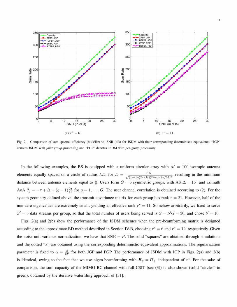
Fig. 2. Comparison of sum spectral efficiency (bit/s/Hz) vs. SNR (dB) for JSDM with their corresponding deterministic equivalents. “JGP”

denotes JSDM with joint group processing and “PGP” denotes JSDM with per-group processing.

In the following examples, the BS is equipped with a uniform circular array with M = 100 isotropic antenna

elements equally spaced on a circle of radius λD, for D = 0.5√(1−cos(2π/M))2+sin(2π/M)2

, resulting in the minimum

distance between antenna elements equal to λ2 . Users form G = 6 symmetric groups, with AS ∆ = 15o and azimuth

AoA θg = −π + ∆ + (g − 1)2πG for g = 1, . . . , G. The user channel correlation is obtained according to (2). For the

system geometry defined above, the transmit covariance matrix for each group has rank r = 21. However, half of the

non-zero eigenvalues are extremely small, yielding an effective rank r? = 11. Somehow arbitrarily, we fixed to serve

S′ = 5 data streams per group, so that the total number of users being served is S = S′G = 30, and chose b′ = 10.

Figs. 2(a) and 2(b) show the performance of the JSDM schemes when the pre-beamforming matrix is designed

according to the approximate BD method described in Section IV-B, choosing r? = 6 and r? = 12, respectively. Given

the noise unit variance normalization, we have that SNR = P . The solid “squares” are obtained through simulations

and the dotted “x” are obtained using the corresponding deterministic equivalent approximations. The regularization

parameter is fixed to α = SbP for both JGP and PGP. The performance of JSDM with JGP in Figs. 2(a) and 2(b)

is identical, owing to the fact that we use eigen-beamforming with BBBg = UUUg, independent of r?. For the sake of

comparison, the sum capacity of the MIMO BC channel with full CSIT (see (3)) is also shown (solid “circles” in

green), obtained by the iterative waterfiling approach of [31].

15

Remark 5: By choosing r? too small, such that significant eigenmodes are not taken into account by the approx-

imate BD pre-beamforming matrix, the resulting inter-group interference is large and the performance of PGP is

severely interference limited (e.g., Fig. 2(a)). Instead, by choosing r? large enough, in order to include all significant

eigenmodes, the performance of PGP does not show a noticeable interference limited behavior over a wide range of

SNR. This is the case of Fig. 2(b), where we chose r? = 12 and the channel covariance matrix has rank r = 21,

but only 11 significant eigenvalues. As a matter of fact, the PGP rate curves of Fig. 2(b) will eventually flatten,

but this happens at extremely large SNR, irrelevant for practical applications. This example shows that r? should

always be chosen in order to include all strongest eigenmodes. However, making r? = r is generally not a good

choice since many eigenmodes may be very close to zero (as in this example) and therefore including them in the

count of r? yields a dimensionality bottleneck without any real benefit in terms of inter-group interference (recall

that r?G ≤ M , therefore if r? is large we may have to decrease G, i.e., serve less groups in parallel). We conclude

that the choice of the effective rank r? should be carefully optimized, depending on the specific channel covariance

eigenvalue distribution. ♦

VI. DOWNLINK TRAINING AND NOISY CSIT

In this section, we evaluate the impact of noisy CSIT by including the fact that the effective channels are estimated

by the UTs from the downlink training phase. In the vast literature dedicated to CSIT feedback (see for example [3]

and references therein), methods that achieve the estimated channel Mean-Square Error (MSE) decreases as O(1/P β)

for some β ≥ 1, even in the presence of channel feedback noise and errors, are well-known. In contrast, the MSE due

to estimation from the downlink training phase decreases at best as O(1/P ). In fact, this is given by the high-SNR

behavior of the MMSE for a Gaussian signal (the channel vectors) in Gaussian noise. If the CSIT feedback scheme

is designed to achieve exponent β > 1 and the channel SNR is sufficiently large, the feedback error is negligible with

respect to the downlink estimation error [3]. Hence, for simplicity, we consider the optimistic situation of ideal and

delay-free CSIT feedback, and focus only on the effect of the downlink channel estimation error and dimensionality

penalty factor of the training phase (a similar approach is followed in [5]).

For brevity, we focus only on the case of PGP.7 From Section V-B, the channel covariance matrix for a user gk

is given by RRRg = BBBHgRRRgBBBg. In order to estimate the effective channel vector hhhgk , i.e., the column of the effective

channel matrix HHHg corresponding to user gk, the BS sends unitary training sequences of length b′, in parallel over

the b′ virtual inputs of the pre-beamforming of each group g. Hence, the training phase with PGP spans b′ symbols.

The UTs in each group make use of linear MMSE estimation, which is the optimal estimator for minimizing the

7Analogous results can be obtained for the case of JGP, but these are practically less interesting since JGP requires typically too large training

and feedback overhead in FDD systems.

16

MSE since the observation at each user and the channel vector are conditionally jointly Gaussian given the training

sequences. The MMSE channel estimates are fed back to the BS and are used to compute the linear precoders {PPP g}.

Assuming that in each coherence block of T symbols the training phase makes use of b′ symbols, and the remaining

T − b′ symbols are available for downlink data transmission, it follows that the spectral efficiency must be scaled by

the dimensionality penalty factor max{1− b′/T, 0}.

We consider a scheme where a scaled unitary training matrix XXXtr of dimension b′ × b′ is sent, simultaneously, to

all groups in the common downlink training phase. The corresponding received signal at group g receivers is given

by

YYY g = HHHHgXXXtr +

∑g′ 6=g

HHHgHBBBg′XXXtr +ZZZg. (47)

Multiplying from the right by XXXHtr and using the fact that, by design, XXXtrXXX

Htr = ρtrIIIb′ where ρtr is the power allocated

to training, we obtain

YYY gXXXHtr = ρtrHHH

Hg + ρtr

∑g′ 6=g

HHHgHBBBg′ +ZZZgXXX

Htr. (48)

Extracting the gk-th row, dividing by√ρtr, using the fact that ZZZgXXXH

tr has i.i.d. entries ∼ CN (0, ρtr) and taking

Hermitian transpose of everything, we obtain the noisy observation for estimating the gk-th effective channel vector

in the form

hhhgk =√ρtrhhhgk +

√ρtr

∑g′ 6=g

BBBHg′

hhhgk + zzzgk , (49)

where zzzgk ∼ CN (000, IIIb′). The MMSE estimator for hhhgk based on (49) is given by

hhhgk = E[hhhgkhhh

H

gk

]E[hhhgkhhh

H

gk

]−1

hhhgk

=√ρtr

BBBHgRRRg

G∑g′=1

BBBg′

ρtr

G∑g′,g′′=1

BBBHg′RRRgBBBg′′ + IIIb′

−1

hhhgk

=1√ρtr

(MMMgRRRgOOO

T)[OOORRRgOOO

T +1

ρtrIIIb′

]−1

hhhgk (50)

where we used the fact that hhhgk = BBBHg hhhgk , where RRRg is defined in (21) and we introduced the b′ × b block matrices

MMMg = [000, . . . ,000, IIIb′︸︷︷︸block g

,000, . . . ,000]

OOO = [IIIb′ , IIIb′ , . . . , IIIb′ ].

Notice that in the case of perfect BD we have that RRRgBBBg′ = 000 for g′ 6= g. Therefore, (49) and (50) reduce to

hhhgk =√ρtrhhhgk + zzzgk , (51)

17

and

hhhgk =1√ρtrRRRg

[RRRg +

1

ρtrIIIb′

]−1

hhhgk (52)

respectively, where we recall the definition RRRg = BBBHgRRRgBBBg.

For this channel estimation scheme, the deterministic equivalent approximation of the SINR terms for RZFBF and

ZFBF precoding can be obtained following [11], [33], the approach of which can be directly applied to our case, and

using the well-known MMSE decomposition

hhhgk = hhhgk + eeegk , (53)

with E[hhhgkhhhH

gk ] = RRRg and MMSE covariance matrix E[eeegkeeeHgk ] = RRRg− RRRg. For completeness, the fixed-point equations

leading to the deterministic equivalent SINR approximation for PGP with noisy CSIT are given in Appendix A.

Eventually, the achievable rate of user gk is approximated by

Rgk,pgp,csit = max

{1− b′

T, 0

}× log(1 + γogk,pgp,csit), (54)

where γogk,pgp,csit indicates either γogk,pgp,rzf,csit or γogk,pgp,zf,csit, as detailed in Appendix A.

Remark 6: Assuming that, as M → ∞, the other system dimensions r?, S and b also go to infinity linearly with

M , the achievable rate approximation error converges to zero almost surely as M →∞. However, the dimensionality

factor max{1 − b′/T, 0} is equal to zero for b′ ≥ T . Hence, in order to obtain mathematically meaningful results

we assume that also the coherence block length T grows linearly with M , and we define the factor τ = b′/T as the

dimensionality crowding factor of the channel. In practice, this means that the method is valid in the regime of b′

large, but still significantly smaller than T . ♦

A. Results with downlink channel estimation

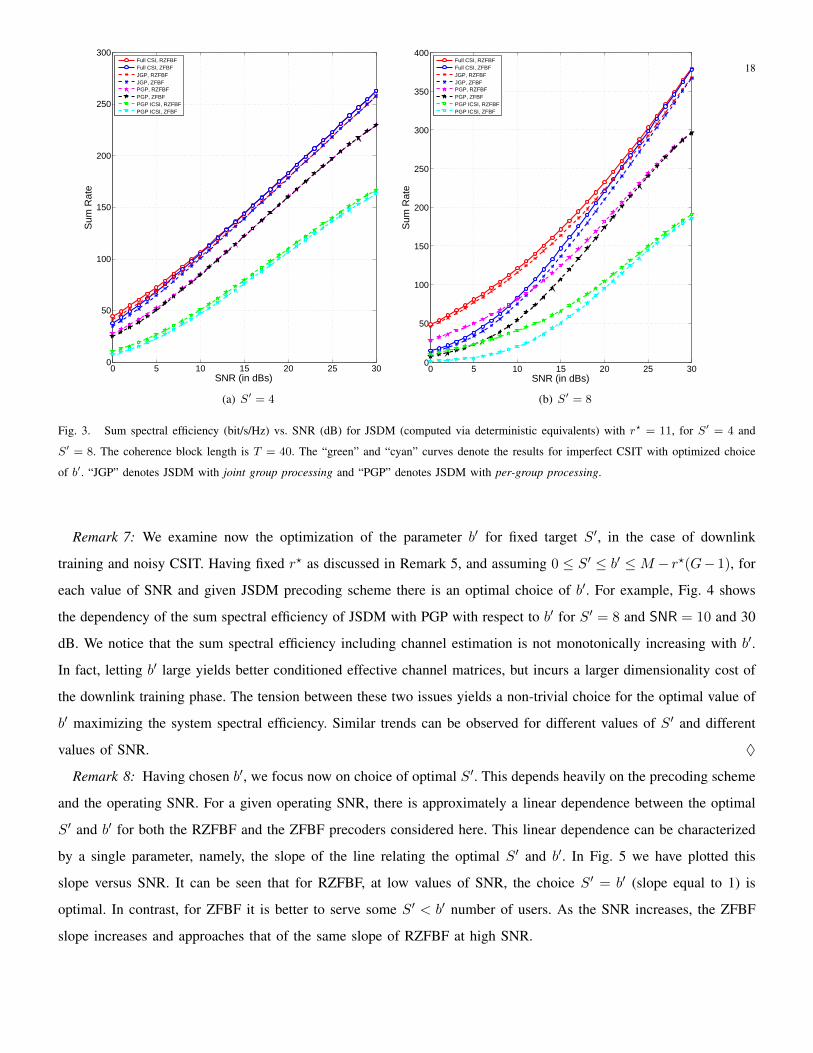
We demonstrate the effect of noisy CSIT on the performance of RZFBF and ZFBF in Fig. 3, for the same antenna

configuration of Section V-C with r? = 11, for S′ = 4 and S′ = 8 streams per group. For the sake of comparison,

the solid “red” (“blue”) curve denotes the sum spectral efficiency achieved by RZFBF (ZFBF) with full noiseless

CSIT, i.e., by computing the precoding matrix in one step, directly from the instantaneous channel matrix HHH . The

dotted lines represent the performance of JSDM for JGP with eigen-beamforming and noiseless CSIT (i.e., perfect

knowledge of the effective channel HHH). The “magenta” (“black”) curves denote the sum spectral efficiency for JSDM

with PGP and approximate BD, also in the case of noiseless CSIT. Finally, the “green” (“cyan”) curves denote the

achievable sum spectral efficiency for JSDM with PGP and noisy CSIT, obtained by downlink training and MMSE

estimation as explained above. These curves are obtained by optimizing the parameter b′, for given S′, r? and SNR.

Since a set of training sequences is sent simultaneously to all groups, the training power is given by ρtr = PG , such

that the total sum power constraint is preserved also during the training phase.

18

0 5 10 15 20 25 300

50

100

150

200

250

300

SNR (in dBs)

Sum

Rat

e

Full CSI, RZFBFFull CSI, ZFBFJGP, RZFBFJGP, ZFBFPGP, RZFBFPGP, ZFBFPGP ICSI, RZFBFPGP ICSI, ZFBF

(a) S′ = 4

0 5 10 15 20 25 300

50

100

150

200

250

300

350

400

SNR (in dBs)

Sum

Rat

e

Full CSI, RZFBFFull CSI, ZFBFJGP, RZFBFJGP, ZFBFPGP, RZFBFPGP, ZFBFPGP ICSI, RZFBFPGP ICSI, ZFBF

(b) S′ = 8

Fig. 3. Sum spectral efficiency (bit/s/Hz) vs. SNR (dB) for JSDM (computed via deterministic equivalents) with r? = 11, for S′ = 4 and

S′ = 8. The coherence block length is T = 40. The “green” and “cyan” curves denote the results for imperfect CSIT with optimized choice

of b′. “JGP” denotes JSDM with joint group processing and “PGP” denotes JSDM with per-group processing.

Remark 7: We examine now the optimization of the parameter b′ for fixed target S′, in the case of downlink

training and noisy CSIT. Having fixed r? as discussed in Remark 5, and assuming 0 ≤ S′ ≤ b′ ≤M − r?(G− 1), for

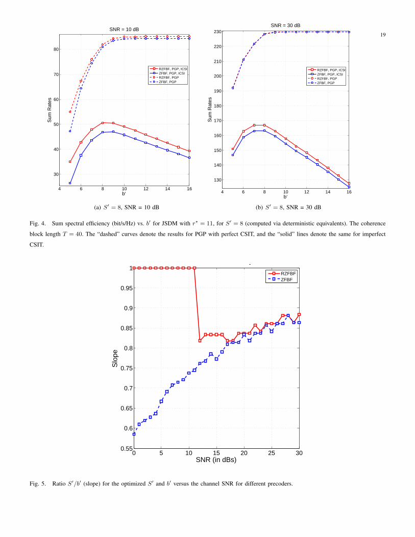
each value of SNR and given JSDM precoding scheme there is an optimal choice of b′. For example, Fig. 4 shows

the dependency of the sum spectral efficiency of JSDM with PGP with respect to b′ for S′ = 8 and SNR = 10 and 30

dB. We notice that the sum spectral efficiency including channel estimation is not monotonically increasing with b′.

In fact, letting b′ large yields better conditioned effective channel matrices, but incurs a larger dimensionality cost of

the downlink training phase. The tension between these two issues yields a non-trivial choice for the optimal value of

b′ maximizing the system spectral efficiency. Similar trends can be observed for different values of S′ and different

values of SNR. ♦

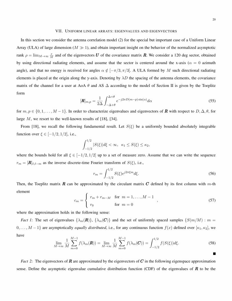
Remark 8: Having chosen b′, we focus now on choice of optimal S′. This depends heavily on the precoding scheme

and the operating SNR. For a given operating SNR, there is approximately a linear dependence between the optimal

S′ and b′ for both the RZFBF and the ZFBF precoders considered here. This linear dependence can be characterized

by a single parameter, namely, the slope of the line relating the optimal S′ and b′. In Fig. 5 we have plotted this

slope versus SNR. It can be seen that for RZFBF, at low values of SNR, the choice S′ = b′ (slope equal to 1) is

optimal. In contrast, for ZFBF it is better to serve some S′ < b′ number of users. As the SNR increases, the ZFBF

slope increases and approaches that of the same slope of RZFBF at high SNR.

19

4 6 8 10 12 14 16

30

40

50

60

70

80

b‘

Sum

Rat

es

SNR = 10 dB

RZFBF, PGP, ICSIZFBF, PGP, ICSIRZFBF, PGPZFBF, PGP

(a) S′ = 8, SNR = 10 dB

4 6 8 10 12 14 16

130

140

150

160

170

180

190

200

210

220

230

b‘

Sum

Rat

es

SNR = 30 dB

RZFBF, PGP, ICSIZFBF, PGP, ICSIRZFBF, PGPZFBF, PGP

(b) S′ = 8, SNR = 30 dB

Fig. 4. Sum spectral efficiency (bit/s/Hz) vs. b′ for JSDM with r? = 11, for S′ = 8 (computed via deterministic equivalents). The coherence

block length T = 40. The “dashed” curves denote the results for PGP with perfect CSIT, and the “solid” lines denote the same for imperfect

CSIT.

0 5 10 15 20 25 300.55

0.6

0.65

0.7

0.75

0.8

0.85

0.9

0.95

1

SNR (in dBs)

Slo

pe

M = 500, Circular Array

RZFBFZFBF

Fig. 5. Ratio S′/b′ (slope) for the optimized S′ and b′ versus the channel SNR for different precoders.

20

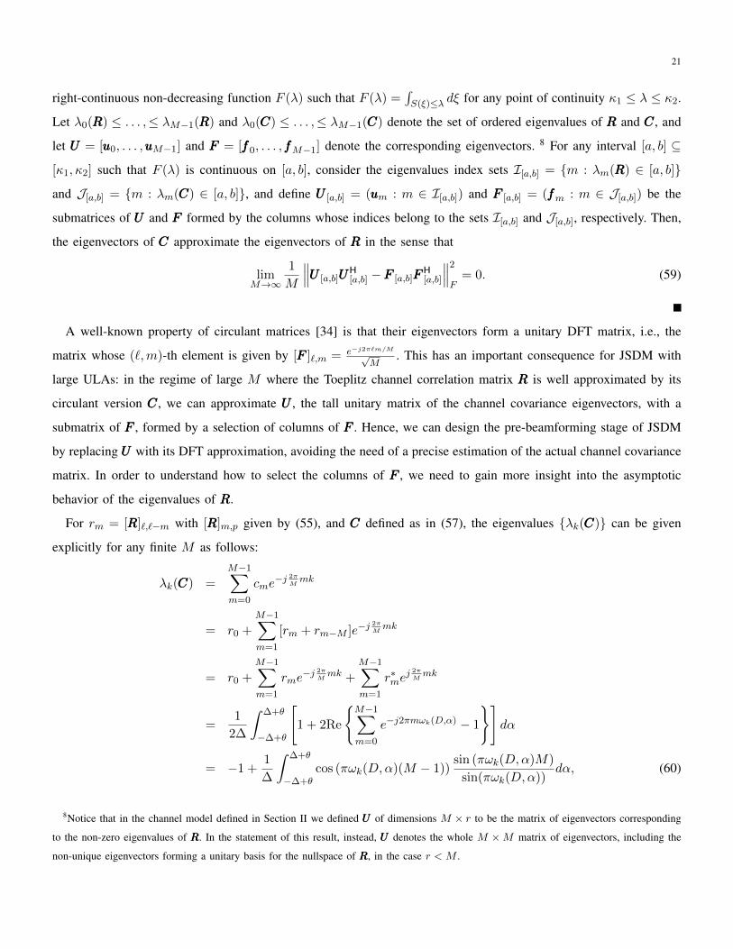
VII. UNIFORM LINEAR ARRAYS: EIGENVALUES AND EIGENVECTORS

In this section we consider the antenna correlation model (2) for the special but important case of a Uniform Linear

Array (ULA) of large dimension (M � 1), and obtain important insight on the behavior of the normalized asymptotic

rank ρ = limM→∞rM and of the eigenvectors UUU of the covariance matrix RRR. We consider a 120 deg sector, obtained

by using directional radiating elements, and assume that the sector is centered around the x-axis (α = 0 azimuth

angle), and that no energy is received for angles α /∈ [−π/3, π/3]. A ULA formed by M such directional radiating

elements is placed at the origin along the y-axis. Denoting by λD the spacing of the antenna elements, the covariance

matrix of the channel for a user at AoA θ and AS ∆ according to the model of Section II is given by the Toeplitz

form

[RRR]m,p =1

2∆

∫ ∆+θ

−∆+θe−j2πD(m−p) sin(α)dα (55)

for m, p ∈ {0, 1, . . . ,M − 1}. In order to characterize eigenvalues and eigenvectors of RRR with respect to D,∆, θ, for

large M , we resort to the well-known results of [18], [34].

From [18], we recall the following fundamental result. Let S(ξ) be a uniformly bounded absolutely integrable

function over ξ ∈ [−1/2, 1/2], i.e., ∫ 1/2

−1/2|S(ξ)|dξ <∞, κ1 ≤ S(ξ) ≤ κ2,

where the bounds hold for all ξ ∈ [−1/2, 1/2] up to a set of measure zero. Assume that we can write the sequence

rm = [RRR]`,`−m as the inverse discrete-time Fourier transform of S(ξ), i.e.,

rm =

∫ 1/2

−1/2S(ξ)ej2πξmdξ. (56)

Then, the Toeplitz matrix RRR can be approximated by the circulant matrix CCC defined by its first column with m-th

element

cm =

rm + rm−M for m = 1, . . . ,M − 1

r0 for m = 0, (57)

where the approximation holds in the following sense:

Fact 1: The set of eigenvalues {λm(RRR)}, {λm(CCC)} and the set of uniformly spaced samples {S(m/M) : m =

0, . . . ,M − 1} are asymptotically equally distributed, i.e., for any continuous function f(x) defined over [κ1, κ2], we

have

limM→∞

1

M

M−1∑m=0

f(λm(RRR)) = limM→∞

1

M

M−1∑m=0

f(λm(CCC)) =

∫ 1/2

−1/2f(S(ξ))dξ. (58)

Fact 2: The eigenvectors ofRRR are approximated by the eigenvectors ofCCC in the following eigenspace approximation

sense. Define the asymptotic eigenvalue cumulative distribution function (CDF) of the eigenvalues of RRR to be the

21

right-continuous non-decreasing function F (λ) such that F (λ) =∫S(ξ)≤λ dξ for any point of continuity κ1 ≤ λ ≤ κ2.

Let λ0(RRR) ≤ . . . ,≤ λM−1(RRR) and λ0(CCC) ≤ . . . ,≤ λM−1(CCC) denote the set of ordered eigenvalues of RRR and CCC, and

let UUU = [uuu0, . . . ,uuuM−1] and FFF = [fff0, . . . , fffM−1] denote the corresponding eigenvectors. 8 For any interval [a, b] ⊆

[κ1, κ2] such that F (λ) is continuous on [a, b], consider the eigenvalues index sets I[a,b] = {m : λm(RRR) ∈ [a, b]}

and J[a,b] = {m : λm(CCC) ∈ [a, b]}, and define UUU [a,b] = (uuum : m ∈ I[a,b]) and FFF [a,b] = (fffm : m ∈ J[a,b]) be the

submatrices of UUU and FFF formed by the columns whose indices belong to the sets I[a,b] and J[a,b], respectively. Then,

the eigenvectors of CCC approximate the eigenvectors of RRR in the sense that

limM→∞

1

M

∥∥∥UUU [a,b]UUUH[a,b] −FFF [a,b]FFF

H[a,b]

∥∥∥2

F= 0. (59)

A well-known property of circulant matrices [34] is that their eigenvectors form a unitary DFT matrix, i.e., the

matrix whose (`,m)-th element is given by [FFF ]`,m = e−j2π`m/M√M

. This has an important consequence for JSDM with

large ULAs: in the regime of large M where the Toeplitz channel correlation matrix RRR is well approximated by its

circulant version CCC, we can approximate UUU , the tall unitary matrix of the channel covariance eigenvectors, with a

submatrix of FFF , formed by a selection of columns of FFF . Hence, we can design the pre-beamforming stage of JSDM

by replacing UUU with its DFT approximation, avoiding the need of a precise estimation of the actual channel covariance

matrix. In order to understand how to select the columns of FFF , we need to gain more insight into the asymptotic

behavior of the eigenvalues of RRR.

For rm = [RRR]`,`−m with [RRR]m,p given by (55), and CCC defined as in (57), the eigenvalues {λk(CCC)} can be given

explicitly for any finite M as follows:

λk(CCC) =

M−1∑m=0

cme−j 2π

Mmk

= r0 +

M−1∑m=1

[rm + rm−M ]e−j2π

Mmk

= r0 +

M−1∑m=1

rme−j 2π

Mmk +

M−1∑m=1

r∗mej 2π

Mmk

=1

2∆

∫ ∆+θ

−∆+θ

[1 + 2Re

{M−1∑m=0

e−j2πmωk(D,α) − 1

}]dα

= −1 +1

∆

∫ ∆+θ

−∆+θcos (πωk(D,α)(M − 1))

sin (πωk(D,α)M)

sin(πωk(D,α))dα, (60)

8Notice that in the channel model defined in Section II we defined UUU of dimensions M × r to be the matrix of eigenvectors corresponding

to the non-zero eigenvalues of RRR. In the statement of this result, instead, UUU denotes the whole M ×M matrix of eigenvectors, including the

non-unique eigenvectors forming a unitary basis for the nullspace of RRR, in the case r < M .

22

where we define the quantity ωk(D,α) = D sin(α) + k/M .

In order to obtain the limiting CDF of the eigenvalues of RRR and find a simple formula for the asymptotic rank ρ,

we obtain an explicit expression of S(ξ) for the autocorrelation function rm = [RRR]`,`−m. Using (55) and invoking the

Lebesgue dominated convergence theorem, we have

S(ξ) =

∞∑m=−∞

rme−j2πξm

=1

2∆

∫ ∆+θ

−∆+θ

[ ∞∑m=−∞

e−j2πm(D sin(α)+ξ)

]dα

(a)=

1

2∆

∫ ∆+θ

−∆+θ

[ ∞∑m=−∞

δ(D sin(α) + ξ −m)

]dα

(b)=

1

2∆

∫ D sin(∆+θ)

D sin(−∆+θ)

[ ∞∑m=−∞

δ(z + ξ −m)

]dz√

D2 − z2, (61)

where in (a) we used the Poisson sum formula (also known as “picked fence miracle” [35]), in (b) we made the

change of variable z = D sin(α). The expression (61) is valid for −π2 ≤ θ−∆ < θ+∆ ≤ π

2 . A more general formula,

able to recover the classical Bessel J0 autocorrelation function [36] in the case of uniform isotropic scattering, is

provided in Appendix B. Owing to the property of the Dirac delta function, we arrive at

S(ξ) =1

2∆

∑m∈[D sin(−∆+θ)+ξ,D sin(∆+θ)+ξ]

1√D2 − (m− ξ)2

. (62)

We have:

Lemma 1: The function S(ξ) is non-constant over its support and uniformly bounded, provided that D ∈ [0, 1/2]

and −φ ≤ θ −∆ < θ + ∆ ≤ φ for some constant angle φ ∈ [0, π/2).

Proof: S(ξ) is periodic and it is sufficient to restrict ξ to the interval [−1/2, 1/2]. As observed before, if

−π2 ≤ θ −∆ < θ + ∆ ≤ π

2 , the general expression of S(ξ) given in Appendix B coincides with (62), and we have

−D < −D sin(φ) ≤ D sin(−∆ + θ) < D sin(∆ + θ) ≤ D sin(φ) < D. Since −1/2 ≤ ξ ≤ 1/2 and D ∈ [0, 1/2], the

following inequalities hold:

D sin(−∆ + θ) + ξ ≥ D sin(−∆ + θ)− 1/2 > −D − 1/2 ≥ −1

D sin(∆ + θ) + ξ ≤ D sin(∆ + θ) + 1/2 < D + 1/2 ≤ 1.

Since −1 < D sin(−∆+θ)+ξ < D sin(∆+θ)+ξ < 1, the only integer in the interval [D sin(−∆+θ)+ξ,D sin(∆+

θ) + ξ] is 0. Thus,

S(ξ) =1

2∆

∑0∈[D sin(−∆+θ)+ξ,D sin(∆+θ)+ξ]

1√D2 − ξ2

. (63)

The support S of S(ξ) is the set of values ξ ∈ [−1/2, 1/2] for which the interval [D sin(−∆+θ)+ξ,D sin(∆+θ)+ξ]

contains the point 0, i.e., S = [−D sin(∆ + θ),−D sin(−∆ + θ)]. It is clear by inspection that S(ξ) is not constant

23

over S (it is sufficient to observe that S(ξ) is differentiable, and its derivative is not identically zero over a set of

non-zero measure). To prove that S(ξ) is uniformly bounded, it is sufficient to notice that the term 1√D2−ξ2 in (63) is

real, continuous and finite for all ξ ∈ (−D,D) ⊃ [−D sin(φ), D sin(φ)] ⊇ S. Hence, it attains its minimum κ′ and

maximum κ2 on S, and these are uniformly bounded as 9

1

D≤ κ′ < κ2 ≤

1

D cos(φ)<∞.

Notice that the assumptions of Lemma 1 are satisfied for antenna spacing not larger than λ/2 and in the assumption,

made here, that the ULA receives/transmits energy only in a 120 deg sector (i.e., for AoAs in [−π/3, π/3]). As a

corollary of (62), we obtain the asymptotic rank in closed form:

Theorem 2: The asymptotic normalized rank of the channel covariance matrix RRR with elements defined in (55),

with antenna separation λD, AoA θ and AS ∆, is given by

ρ = min{1, B(D, θ,∆)}, (64)

where

B(D, θ,∆) = |D sin(−∆ + θ)−D sin(∆ + θ)| . (65)

Proof: Notice that B(D, θ,∆) is the size of the interval for m in the summation appearing in (62). If B(D, θ,∆) ≥

1, for any ξ ∈ [−1/2, 1/2] the sum in (62) is non-empty. It follows that S(ξ) > 0 for all ξ and the asymptotic

normalized rank is ρ = 1. In contrast, if B(D, θ,∆) < 1, there exist a set Sc ⊆ [−1/2, 1/2] of measure 1−B(D, θ,∆)

for which if ξ ∈ Sc then the sum in (62) is empty. Therefore, in this case we have ρ = B(D, θ,∆).

A good approximation of the actual rank r for large but finite M is given by r ≈ ρM , where ρ is given by Theorem 2.

Hence, we can predict accurately the rank of the channel covariance from the system geometric parameters (D, θ,∆).

The empirical CDF of the eigenvalues of RRR is defined by

F(M)RRR (λ) =

1

M

M∑m=1

1{λm(RRR) ≤ λ}. (66)

For large M , F (M)RRR (λ) can be approximated either using (60) or the collection of samples {S([m/M ]) : m =

0, . . . ,M − 1}, where [x] indicates x modulo the interval [−1/2, 1/2]. In both cases, using the resulting collection

of M values in (66), we obtain a convergent approximation F (M)RRR (λ) of the empirical CDF (66) such that [18]

limM→∞

F(M)RRR (λ) = lim

M→∞F

(M)RRR (λ) = F (λ).

9We use κ′ instead of κ1 to denote the minimum of S(ξ) on its support since the minimum eigenvalue, denoted previously by κ1, is generally

equal to 0 whenever S is strictly included in [−1/2, 1/2].

24

0 0.5 1 1.5 2 2.50

0.1

0.2

0.3

0.4

0.5

0.6

0.7

0.8

0.9

1

Eigen Values

CD

F

ToeplitzCirculant, M finiteCirculant, M ∞

Fig. 6. M = 400, θ = π/6, D = 1,∆ = π/10. Exact empirical eigenvalue cdf of RRR (red), its approximation (60) based on the circulant

matrix CCC (dashed blue) and its approximation from the samples of S(ξ) (dashed green).

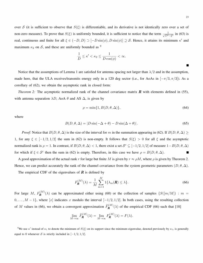
As an example, Fig. 6 shows the exact empirical CDF of RRR, its circulant approximation obtained by (60)) and the

asymptotic approximation obtained from the set {S([m/M ]) : m = 0, . . . ,M−1}, for a specific choice of the system

parameters. It is apparent that, in this regime, both approximations are very accurate.

A. Approximating the channel eigenspace

Going back to the problem of approximating the eigenvectors of RRR with a set of DFT columns, we notice the

following properties of S(ξ) in (62):

1) S(ξ) has support on an interval S ⊆ [−1/2, 1/2], of length ρ (see proof of Theorem 2).

2) S(ξ) is non-constant and bounded over its support (see Lemma 1).

It follows that F (λ) has a single discontinuity at λ = 0, with jump of height 1− ρ, corresponding to the mass-point

of the zero eigenvalues of RRR. For ρ < 1, F (λ) is continuous over (0, κ2] where κ2 = maxS(ξ) <∞ by Lemma 1.

Hence, any interval [a, b] with 0 < a < b ≤ κ2 is a continuity interval of F (λ), and the eigenspace approximation

property of Fact 2 holds. In particular, we have established the following:

25

Corollary 1: Let S denote the support of S(ξ), let JS = {m : [m/M ] ∈ S,m = 0, . . . ,M − 1} be the set of

indices for which the corresponding “angular frequency” ξm = [m/M ] belongs to S, let fffm denote the m-th column

of the unitary DFT matrix FFF , and let FFFS = (fffm : m ∈ JS) be the DFT submatrix containing the columns with

indices in JS . Then,

limM→∞

1

M

∥∥∥UUUUUUH −FFFSFFFHS

∥∥∥2

F= 0, (67)

where UUU is the M × r “tall unitary” matrix of the non-zero eigenvectors of RRR.

Proof: Since S(ξ) is uniformly bounded and strictly positive over S, we have 0 < minξ∈S S(ξ) = κ′ <

maxS(ξ) = κ2. Hence, letting a = κ′ and b = κ2, and using the eigenspace approximation property of Fact 2 yields

the result.

Consider now a JSDM configuration with an ULA serving G groups with AoAs within a 120 deg sector. For

each group g, we can approximate the eigenmodes UUUg by the DFT submatrix FFFSg , where Sg denotes the support of

Sg(ξ), given by (62) for AoA θg and AS ∆ (for simplicity we assume that the AS is common to all groups, although

this can be easily generalized). Corollary (1) implies that if Sg ∩ Sg′ = ∅ (disjoint angular frequency support), then

FFFHSgFFFS′g = 000. It follows that if the G groups are chosen to have spectra with disjoint support, then [FFFS1 , . . . ,FFFSG ]

is exactly tall unitary and, because of Fact 2, UUU = [UUU1, . . . ,UUUG] is approximately tall unitary, for large M . The

following result provides such condition expressed directly in terms of the AoA intervals.

Theorem 3: Groups g and g′ with angle of arrival θg and θg′ and common angular spread ∆ have spectra with

disjoint support if their AoA intervals [θg −∆, θg + ∆] and [θg′ −∆, θg′ + ∆] are disjoint.

Proof: Define:

Ag = max(D sin(θg + ∆), D sin(θg −∆))

Bg = min(D sin(θg + ∆), D sin(θg −∆))

Ag′ = max(D sin(θg′ + ∆), D sin(θg′ −∆))

Bg′ = min(D sin(θg′ + ∆), D sin(θg′ −∆)).

From (62) we notice that Sg(ξ) and Sg′(ξ) have disjoint supports if Ag ≤ Bg′ or Ag′ ≤ Bg. Since the mapping x 7→

sin(x) is one-to-one in the interval [−π/3, π/3], this condition corresponds to [θg−∆, θg+∆]∩ [θg′−∆, θg′+∆] = ∅.

B. DFT pre-beamforming

Owing to the asymptotic eigenspace approximation and mutual orthogonality of the previous section, an efficient

approach to JSDM design when the BS is equipped with a large ULA per sector consists of selecting groups of

users with (almost) identical AoA intervals, and find G groups of such users with non-overlapping AoA intervals.

26

−0.5 0 0.50

1

2

3

4

5

6

7

8

ξ

Eig

en V

alue

s

θ = −45θ = 0θ = 45

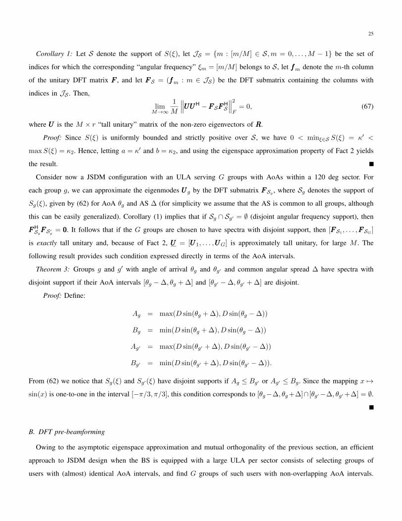
Fig. 7. Eigenvalue spectra for a ULA with M = 400, G = 3, θ1 = −π4, θ2 = 0, θ3 = π

4, D = 1/2 and ∆ = 15 deg.

Then, we let BBBg = FFFSg , for g = 1, . . . , G, with FFFSg defined as in Corollary 1. It follows that FFFHSgUUUg′ ≈ 000 for all

g 6= g′, such that the sum spectral efficiency achieved by JSDM with PGP is close to the sum spectral efficiency

of the corresponding MU-MIMO downlink channel with full CSIT (see Theorem 1). Notice that this approach is

particularly attractive since only a coarse parametric knowledge (AoA interval) for each user is required, rather than

an accurate estimate of its channel covariance matrix.

Fig. 7 show the spectra Sg(ξ) for g = 1, 2, 3, M = 400, and θ1 = −π4 , θ2 = 0, θ3 = π

4 , with D = 1/2 and ∆ = 15

deg. The performance of JSDM with PGP and DFT pre-beamforming is shown in Fig. 8, indicating that up to 20 dB

of SNR, DFT pre-beamforming performs close to schemes with full CSIT.

VIII. JSDM WITH 3D PRE-BEAMFORMING

So far we considered a planar geometry where each user group g is identified by its AoA interval [θg−∆, θg + ∆].

For the sake of simplicity, we allocated equal power to all S downlink data streams. This is a near-optimal power

allocation in the high SNR (high spectral efficiency) regime and in the case where the pathloss from the BS to all

the UTs is approximately equal. In practice, however, users with same (or very similar) AoA interval may be located

at different distances to the BS. In this case, a simple alternative to the complicated and generally non-convex power

27

0 5 10 15 20 25 300

500

1000

1500

SNR

Sum

Rat

e

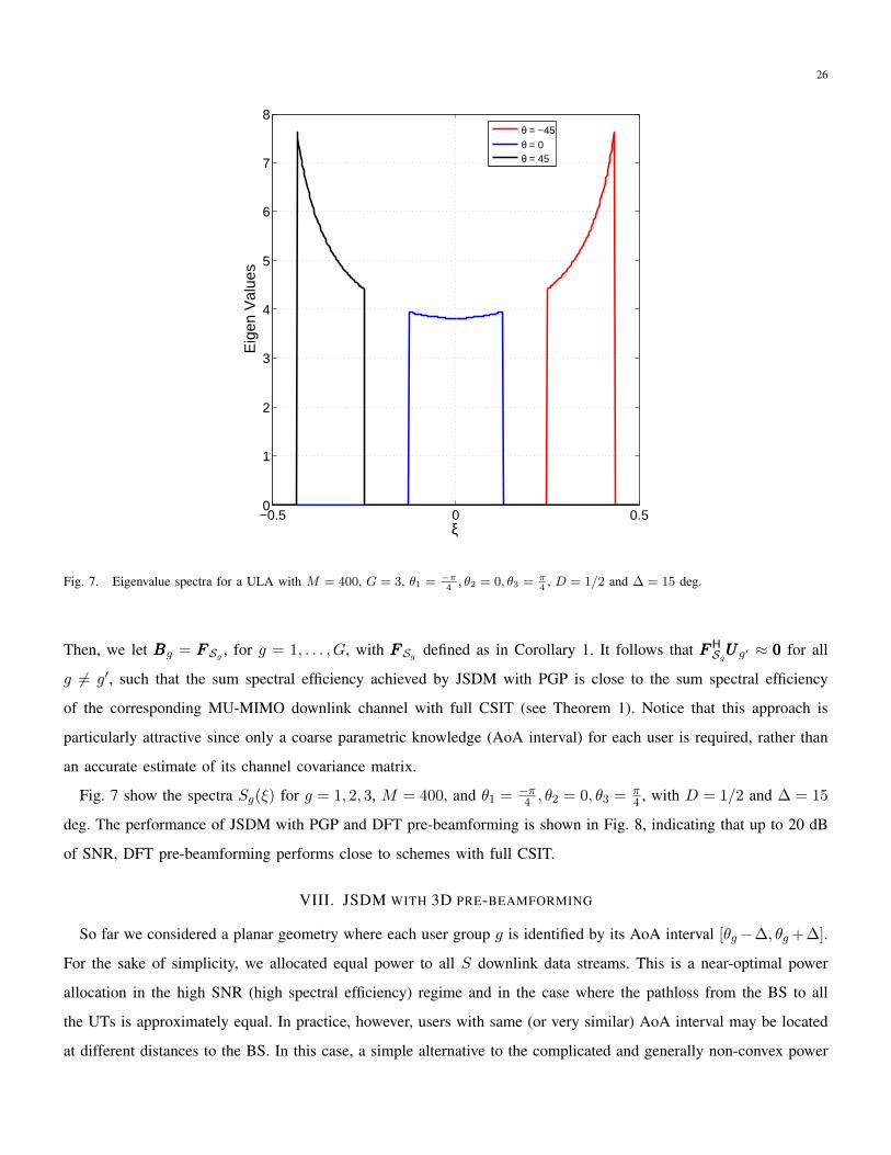
RZFBF, FullZFBF, FullRZFBF, DFTZFBF, DFT

Fig. 8. Sum spectral efficiency (bit/s/Hz) vs. SNR (dB) for JSDM (computed via deterministic equivalents) for DFT pre-beamforming and

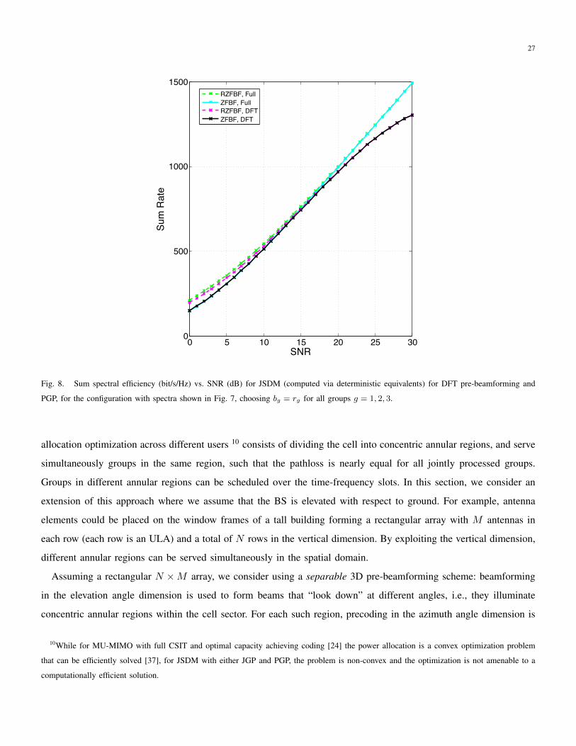
PGP, for the configuration with spectra shown in Fig. 7, choosing bg = rg for all groups g = 1, 2, 3.

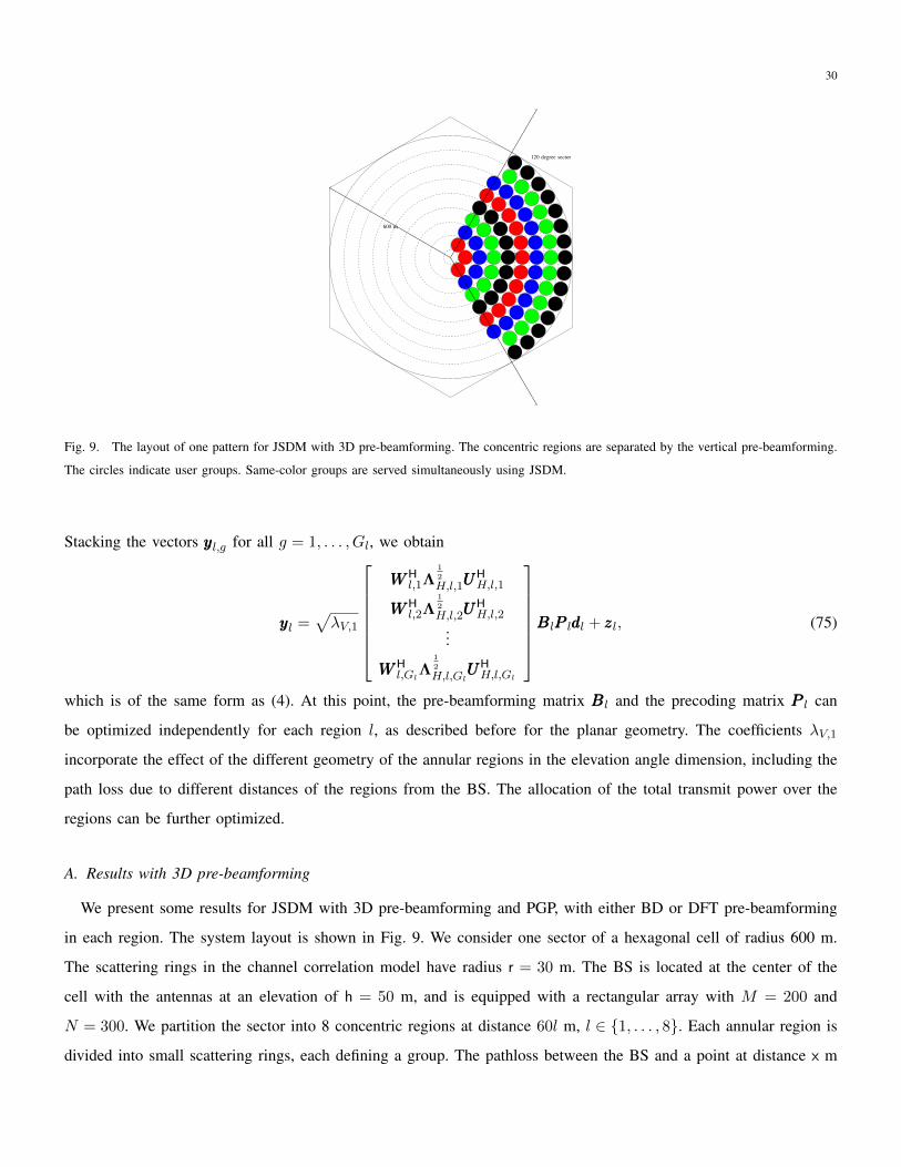
allocation optimization across different users 10 consists of dividing the cell into concentric annular regions, and serve

simultaneously groups in the same region, such that the pathloss is nearly equal for all jointly processed groups.

Groups in different annular regions can be scheduled over the time-frequency slots. In this section, we consider an

extension of this approach where we assume that the BS is elevated with respect to ground. For example, antenna

elements could be placed on the window frames of a tall building forming a rectangular array with M antennas in

each row (each row is an ULA) and a total of N rows in the vertical dimension. By exploiting the vertical dimension,

different annular regions can be served simultaneously in the spatial domain.

Assuming a rectangular N ×M array, we consider using a separable 3D pre-beamforming scheme: beamforming

in the elevation angle dimension is used to form beams that “look down” at different angles, i.e., they illuminate

concentric annular regions within the cell sector. For each such region, precoding in the azimuth angle dimension is

10While for MU-MIMO with full CSIT and optimal capacity achieving coding [24] the power allocation is a convex optimization problem

that can be efficiently solved [37], for JSDM with either JGP and PGP, the problem is non-convex and the optimization is not amenable to a

computationally efficient solution.

28

obtained by JSDM scheme with M antennas, as done before. Thanks to separability, we can optimize JSDM schemes

independently, one for each annular region.

The groups served simultaneously by JSDM in the same region are now identified by two indices, (l, g) where

l = 1, . . . , L indicates the annular region and g = 1, . . . , Gl the group in each l-th region. A set of groups served

simultaneously, on the same time-frequency dimensions, is referred to as a “pattern”. A pattern does not necessarily

cover the whole sector. In fact, it is usually better to allow for “holes” in the pattern, i.e., the group footprints can be

separated by gaps, in order to guarantee near orthogonality between the dominant eigenmodes of the groups in the

same pattern and thus limiting inter-group interference with PGP. In order to provide coverage to the whole sector,

different intertwined patterns can be multiplexed over the time-frequency dimension, similarly to the intertwined

cooperative pattern idea proposed in [38], [39], [40]. The fraction of the time-frequency dimensions allocated to each

pattern can be further optimized in order to maximize a network utility function, reflecting some desired notion of

fairness (see for example [10]).

For the time being, we focus on a single pattern comprising L regions in the elevation angle dimension, and

Gl groups in the azimuth angle dimension for each region l = 1, . . . , L. We let Kl,g denote the number of users

in group (l, g). At the BS, an N ×M rectangular antenna array with N rows and M columns is used. For each

region l, we denote by RRRV,l ∈ CN×N the vertical channel covariance matrix 11 and, for each group (l, g), we let

RRRH,l,g ∈ CM×M denote the the horizontal channel covariance matrix. RRRV,l and RRRH,l,g are modeled according to (2),

with the eigen-decompositions:

RRRV,l = UUUV,lΛV,lUUUHV,l, and RRRH,l,g = UUUH,l,gΛH,l,gUUU

HH,l,g. (68)

Letting hhhl,gk denote the MN × 1 the vectorized channel from the M ×N BS array to the kth user in group (l, g),

we have

E[hhhl,gkhhhHl,gk ] = RRRl,g = RRRH,l,g ⊗RRRV,l = (UUUH,l,g ⊗UUUV,l)(ΛH,l,g ⊗ΛV,l)(UUU

HH,l,g ⊗UUUH

V,l). (69)

This covariance matrix is common (by assumption) to all users gk in group (l, g). Denoting the ranks of RRRH,l,g and

RRRV,l by rH,l,g and rV,l, respectively, we write hhhl,gk as

hhhl,gk = (UUUH,l,g ⊗UUUV,l)(Λ1

2

H,l,g ⊗Λ1

2

V,l)wwwl,gk ,

where UUUH,l,g is M × rH,l,g, UUUV,l is N × rV,l, ΛH,l,g is rH,l,g × rH,l,g and ΛV,l is rV,l × rV,l. The vector wwwl,gk , of

dimension rH,l,grV,l × 1, has i.i.d. entries ∼ CN (0, 1).

In JSDM with 3D pre-beamforming, the transmitted signal is given by

xxx =

L∑l=1

(BBBlPPP ldddl)⊗ qqql, (70)

11We assume that the vertical correlation does not depend on g, but just on l.

29

where qqql denotes the N × 1 pre-beamforming vector for region l in the elevation angle dimension, BBBl is the M × blpre-beamforming matrix of the form BBBl = [BBBl,1, . . . ,BBBl,Gl ], where BBBl,g denotes the pre-beamforming matrix of

size M × bl,g for group (l, g) and PPP l is the linear precoding matrix for the groups of region l, that depends on

the instantaneous effective channels as given in Section III. Notice that we allocate (by design) a single dimension

per region in the elevation angle direction (this is why qqql has dimensions N × 1) since, because of the relatively

small angle under which the BS sees the different regions, it is realistic to expect that RRRV,l has a single dominant

eigenmode. Generalizations considering higher dimensional vertical pre-beamforming for each region are conceptually

straightforward, although not very useful in typical practical scenarios.

Using repeatedly the Kronecker product rule (AAA⊗BBB)(CCC ⊗DDD) = (AAACCC)⊗ (BBBDDD), the received signal for user gk in

group (l, g) can be written as

yl,gk = wwwHl,gk(Λ

1

2

H,l,g ⊗Λ1

2

V,l)(UUUHH,l,g ⊗UUUH

V,l)xxx+ zl,gk

= wwwHl,gk(Λ

1

2

H,l,g ⊗Λ1

2

V,l)(UUUHH,l,g ⊗UUUH

V,l)

[L∑

m=1

(BBBmPPPmdddm)⊗ qqqm

]+ zl,gk

= wwwHl,gk(Λ

1

2

H,l,g ⊗Λ1

2

V,l)

L∑m=1

[(UUUH

H,l,gBBBmPPPmdddm)⊗ (UUUHV,lqqqm)

]+ zl,gk

= wwwHl,gk(Λ

1

2

H,l,g ⊗Λ1

2

V,l)

L∑m=1

[(UUUH

H,l,gBBBm)⊗ (UUUHV,lqqqm)

]PPPmdddm + zl,gk . (71)

If qqqm is chosen to be orthogonal to Span({UUUV,l : l 6= m}), (71) reduces to

yl,gk = wwwHl,gk(Λ

1

2

H,l,g ⊗Λ1

2

V,l)[(UUUH

H,l,gBBBl)⊗ (UUUHV,lqqql)

]PPP ldddl + zl,gk . (72)

Stacking the signals yl,gk for all users gk in group (l, g) into a Kl,g × 1 vector yyyl,g, we obtain

yyyl,g = WWWHl,g(Λ

1

2

H,l,g ⊗Λ1

2

V,l)[(UUUH

H,l,gBBBl)⊗ (UUUHV,lqqql)

]PPP ldddl + zzzl,g, (73)

where we let WWW l,g = [wwwl,g1 , . . . ,wwwl,gKl,g ] and zzzl,g = [zl,g1 , . . . , zl,gKl,g ]T.

If the regions are sufficiently separated in the elevation angle dimension, it is possible to align qqql with the dominant

eigenmode of UUUV,l, while maintaining the orthogonality condition UUUHV,mqqql = 0 for m 6= l. In this case, we have

UUUHV,lqqql = (1, 0, . . . , 0)T and (73) reduces to the same form treated previously for the planar geometry, with an

additional region-specific coefficient√λV,1, corresponding to the largest eigenvalue of the matrix ΛV,l:

yyyl,g =√λV,1WWW

Hl,gΛ

1

2

H,l,gUUUHH,l,gBBBlPPP ldddl + zzzl,g. (74)

300

600 m

50 m

120 degree sector

Fig. 9. The layout of one pattern for JSDM with 3D pre-beamforming. The concentric regions are separated by the vertical pre-beamforming.

The circles indicate user groups. Same-color groups are served simultaneously using JSDM.

Stacking the vectors yyyl,g for all g = 1, . . . , Gl, we obtain

yyyl =√λV,1

WWWH

l,1Λ1

2

H,l,1UUUHH,l,1

WWWHl,2Λ

1

2

H,l,2UUUHH,l,2

...

WWWHl,GlΛ

1

2

H,l,GlUUUHH,l,Gl

BBBlPPP ldddl + zzzl, (75)

which is of the same form as (4). At this point, the pre-beamforming matrix BBBl and the precoding matrix PPP l can

be optimized independently for each region l, as described before for the planar geometry. The coefficients λV,1

incorporate the effect of the different geometry of the annular regions in the elevation angle dimension, including the

path loss due to different distances of the regions from the BS. The allocation of the total transmit power over the

regions can be further optimized.

A. Results with 3D pre-beamforming

We present some results for JSDM with 3D pre-beamforming and PGP, with either BD or DFT pre-beamforming

in each region. The system layout is shown in Fig. 9. We consider one sector of a hexagonal cell of radius 600 m.

The scattering rings in the channel correlation model have radius r = 30 m. The BS is located at the center of the

cell with the antennas at an elevation of h = 50 m, and is equipped with a rectangular array with M = 200 and

N = 300. We partition the sector into 8 concentric regions at distance 60l m, l ∈ {1, . . . , 8}. Each annular region is

divided into small scattering rings, each defining a group. The pathloss between the BS and a point at distance x m

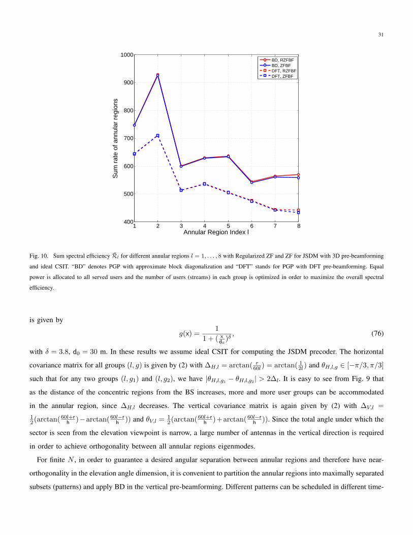
31

1 2 3 4 5 6 7 8400

500

600

700

800

900

1000

Annular Region Index l

Sum

rat

e of

ann

ular

reg

ions

BD, RZFBFBD, ZFBFDFT, RZFBFDFT, ZFBF

Fig. 10. Sum spectral efficiency Rl for different annular regions l = 1, . . . , 8 with Regularized ZF and ZF for JSDM with 3D pre-beamforming

and ideal CSIT. “BD” denotes PGP with approximate block diagonalization and “DFT” stands for PGP with DFT pre-beamforming. Equal

power is allocated to all served users and the number of users (streams) in each group is optimized in order to maximize the overall spectral

efficiency.

is given by

g(x) =1

1 + ( xd0

)δ, (76)

with δ = 3.8, d0 = 30 m. In these results we assume ideal CSIT for computing the JSDM precoder. The horizontal

covariance matrix for all groups (l, g) is given by (2) with ∆H,l = arctan( r60l ) = arctan( 1

2l ) and θH,l,g ∈ [−π/3, π/3]

such that for any two groups (l, g1) and (l, g2), we have |θH,l,g1 − θH,l,g2 | > 2∆l. It is easy to see from Fig. 9 that

as the distance of the concentric regions from the BS increases, more and more user groups can be accommodated

in the annular region, since ∆H,l decreases. The vertical covariance matrix is again given by (2) with ∆V,l =

12(arctan(60l+r

h )−arctan(60l−rh )) and θV,l = 1

2(arctan(60l+rh )+arctan(60l−r

h )). Since the total angle under which the

sector is seen from the elevation viewpoint is narrow, a large number of antennas in the vertical direction is required

in order to achieve orthogonality between all annular regions eigenmodes.

For finite N , in order to guarantee a desired angular separation between annular regions and therefore have near-

orthogonality in the elevation angle dimension, it is convenient to partition the annular regions into maximally separated

subsets (patterns) and apply BD in the vertical pre-beamforming. Different patterns can be scheduled in different time-

32

frequency slots. We denote by A = {A1,A2, . . .} the set of patterns. Finding the best possible pattern partition is

computationally hard, so for the sake of simplicity, we consider a simple partitioning as shown in Fig. 9, where

annular regions with the same color belong to the same pattern. In our example (see Fig. 9), numbering the annular

regions in ascending order based on their proximity to the BS, we have A = {{1, 5}, {2, 6}, {3, 7}, {4, 8}}. In this

way, (75) is replaced by

yyyl = |Λ1

2

V,lUUUHV,lqqql|

WWWH

l,1Λ1

2

H,l,1UUUHH,l,1

WWWHl,2Λ

1

2

H,l,2UUUHH,l,2

...

WWWHl,GlΛ

1

2

H,l,GlUUUHH,l,Gl

BBBlPPP ldddl + zzzl. (77)

Notice that due to BD in the vertical direction, the inter-region interference is exactly zero since UUUHV,mqqql = 000 for

m 6= l. Within each annular region, we use JSDM with PGP. The pre-beamforming matrices BBBl for region l are

obtained using approximate BD or the DFT method, as discussed in previous sections. The dominant rank r?l,g for

each group (l, g) is given by

r?l,g = MD(sin(θH,l,g + ∆H,l)− sin(θH,l,g −∆H,l)), (78)

which is a good approximation for large M motivated by Theorem 2. For simplicity, we do not consider noisy CSIT

and assume that the BS has full knowledge of the effective channels. Hence, we let bl,g = r?l,g. In contrast, in the

case of noisy CSIT the parameter bl,g should be optimized for given channel coherence block length T , as discussed

in Remark 7.

Denoting by Rq the sum spectral efficiency of pattern Aq, and letting Q denote the number of patterns, the network

utility maximization problem is given by

max g(R1, . . . ,RQ)

subject to Rq ≤ νqR∗q , for q = 1, . . . , Q,

Q∑q=1

νq = 1. (79)

where g(·) is a concave component-wise non-decreasing network utility function capturing some desired notion of

fairness, and the optimization variables {νq} are the fractions of time-frequency dimensions allocated to each pattern.

We define

R∗q =∑l∈Aq

Gl∑g=1

Sl,g∑k=1

Rl,g,k,

to be the spectral efficiency of each individual pattern, where Sl,g is the number of downlink streams to group (l, g)

and Rl,g,k is the rate of the k-th stream of group (l, g). We have considered two cases of fairness: proportional fairness

(PFS), and max-min fairness. In both cases, the optimal dimension allocation fractions {νq} can be found in closed

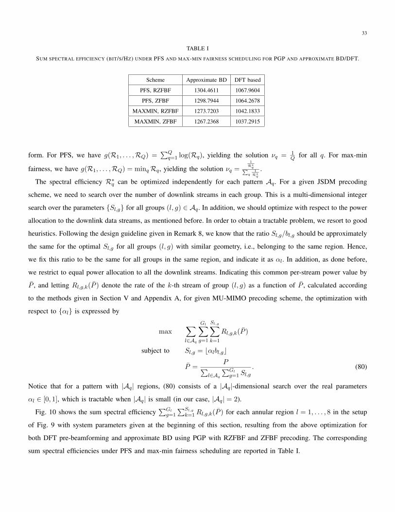
33

TABLE I

SUM SPECTRAL EFFICIENCY (BIT/S/HZ) UNDER PFS AND MAX-MIN FAIRNESS SCHEDULING FOR PGP AND APPROXIMATE BD/DFT.

Scheme Approximate BD DFT based

PFS, RZFBF 1304.4611 1067.9604

PFS, ZFBF 1298.7944 1064.2678

MAXMIN, RZFBF 1273.7203 1042.1833

MAXMIN, ZFBF 1267.2368 1037.2915

form. For PFS, we have g(R1, . . . ,RQ) =∑Q

q=1 log(Rq), yielding the solution νq = 1Q for all q. For max-min

fairness, we have g(R1, . . . ,RQ) = minqRq, yielding the solution νq =1

R∗q∑q

1

R∗q

.

The spectral efficiency R∗q can be optimized independently for each pattern Aq. For a given JSDM precoding

scheme, we need to search over the number of downlink streams in each group. This is a multi-dimensional integer

search over the parameters {Sl,g} for all groups (l, g) ∈ Aq. In addition, we should optimize with respect to the power

allocation to the downlink data streams, as mentioned before. In order to obtain a tractable problem, we resort to good

heuristics. Following the design guideline given in Remark 8, we know that the ratio Sl,g/bl,g should be approximately

the same for the optimal Sl,g for all groups (l, g) with similar geometry, i.e., belonging to the same region. Hence,

we fix this ratio to be the same for all groups in the same region, and indicate it as αl. In addition, as done before,

we restrict to equal power allocation to all the downlink streams. Indicating this common per-stream power value by

P , and letting Rl,g,k(P ) denote the rate of the k-th stream of group (l, g) as a function of P , calculated according

to the methods given in Section V and Appendix A, for given MU-MIMO precoding scheme, the optimization with

respect to {αl} is expressed by

max∑l∈Aq

Gl∑g=1

Sl,g∑k=1

Rl,g,k(P )

subject to Sl,g = bαlbl,gc

P =P∑

l∈Aq∑Gl

g=1 Sl,g. (80)

Notice that for a pattern with |Aq| regions, (80) consists of a |Aq|-dimensional search over the real parameters

αl ∈ [0, 1], which is tractable when |Aq| is small (in our case, |Aq| = 2).

Fig. 10 shows the sum spectral efficiency∑Gl

g=1

∑Sl,gk=1Rl,g,k(P ) for each annular region l = 1, . . . , 8 in the setup

of Fig. 9 with system parameters given at the beginning of this section, resulting from the above optimization for

both DFT pre-beamforming and approximate BD using PGP with RZFBF and ZFBF precoding. The corresponding

sum spectral efficiencies under PFS and max-min fairness scheduling are reported in Table I.

34

IX. CONCLUDING REMARKS

In this work we proposed Joint Space-Division and Multiplexing (JSDM), a novel approach to MU-MIMO downlink

that requires reduced channel estimation downlink training overhead and CSIT feedback and therefore is potentially

suited to FDD systems, despite using a large number of BS antennas. JSDM exploits the fact that for large BSs,

mounted on the top of a building or on a dedicated tower, channel vectors are far from isotropically distributed.

Instead, their dominant eigenspace has dimension much smaller than the number of BS antennas. Different groups

of users are selected, such that the users in each group share (approximately) the same dominant eigenspace, and

the eigenspaces of different groups are nearly orthogonal. JSDM serves simultaneously such groups of users, and

multiple users in each group. The separation of the groups in the spatial domain (space-division) is obtained through

a pre-beamforming matrix that depends only on the channel covariance matrices, while the multiplexing of multiple

users in each group is obtained via linear MU-MIMO precoding based on the instantaneous “effective” channel,

including the pre-beamforming. It turns out that the effective channel has reduced dimensionality with respect to

the original multi-antenna multiuser channel, especially with a “per-group processing” (PGP) approach, i.e., where

each group is individually pre-coded, disregarding the inter-group interference. JSDM with PGP can be regarded as a

generalization of sectorization, where each group acts as a directional sector, and in each sector we apply MU-MIMO

spatial multiplexing, disregarding inter-sector interference.

We showed that when the collection of the channel covariance eigenvectors of the groups forms a tall unitary matrix,

then JSDM with PGP is optimal, in the sense that it can achieve the capacity of the underlying MU-MIMO channel

with full instantaneous CSIT. Then, using Szego’s asymptotic theory of large Toeplitz random matrices, we showed

that when the BS is equipped with a large linear uniform array, this tall unitary condition is closely approached, and

the pre-beamforming matrix can be obtained by selecting an appropriate subset of columns of a unitary DFT matrix.

In fact, under these assumptions the accurate estimation of the channel covariance matrix is not needed, and just a

coarse estimation of the AoA range for each group is sufficient, as long as the AoA ranges of different groups do not

overlap in the azimuth angle domain. Finally, we extended our approach to the case of 3D beamforming, considering

rectangular arrays and pre-beamforming in the elevation angle (vertical) direction. In this case, the proposed JSDM

scheme partitions the cell into concentric annular regions, and serves groups of users with different azimuth angle

in each region. We demonstrated the effectiveness of the proposed scheme in the case of a typical cell size, typical

propagation pathloss, and a large rectangular antenna array mounted on the face of a tall building. In our case, under

ideal CSIT, unprecedented spectral efficiencies of the order of 1000 bit/s/Hz per sector are achieved under various

fairness criteria and pre-beamforming techniques.

We also considered the problem of downlink channel estimation and provided formulas for the asymptotic “deter-

ministic equivalent” approximation of the achievable receiver SINR, which allows efficient calculation of the system

35

performance without resorting to lengthy Monte Carlo simulation. For a realistic SNR range around 20 dB, the effect

of noisy CSIT can be quantified in ≈ 30% loss with respect to the ideal CSIT case. Hence, spectral efficiencies of

≈ 700 bit/s/Hz can be expected for the massive 3D JSDM system scenario.

The design of a JSDM system involves many choices: effective rank r?g of the channel covariance matrix for

each group, pre-beamforming dimension bg, number of users (downlink streams) for each group Sg, for given

pre-beamforming design, operating SNR, and MU-MIMO precoding scheme. In the case of 3D beamforming, this

optimization is significantly more complicated since it has to be repeated for groups of annular regions served

simultaneously by the vertical beamforming. One of the main merits of this paper is to provide simple and solid

design criteria for such a system, based on the insight gained by the asymptotic analysis. In fact, a brute-force search

over the whole parameter space becomes quickly infeasible for practical system scenarios.

We conclude this work by pointing out two interesting related topics, which are left for future work: 1) user

group formation; 2) estimation of the channel covariance matrix dominant eigenspace. User group formation considers

clustering algorithms that, given K users each of which is characterized by its channel covariance dominant eigenspace,

forms groups of users that can be served simultaneously using JSDM, such that the system spectral efficiency is

maximized. In order to enable user group formation and JSDM, the dominant eigenspace of each user must be

estimated from noisy samples of the received signal. Here, the problem is that for a large number of BS antennas

the channel covariance matrix is high-dimensional, and the dimension is typically comparable with the number of

samples. Hence, the common wisdom on “sample covariance” estimation does not apply, and more sophisticated

techniques must be used (e.g., [20, Ch. 17], [15], [17]).

APPENDIX A

DETERMINISTIC EQUIVALENTS FOR THE SINR WITH PGP AND NOISY CSIT

We provide fixed-point equations for the calculation of the deterministic equivalent approximations of the SINR

for JSDM with PGP, noisy CSIT and the two types of linear precoding considered in this paper, namely, RZFBF and

ZFBF. Notice that these expressions hold for arbitrary pre-beamforming matrices, as long as they are fixed constants

independent of the instantaneous channel matrix realizations. In particular, they hold for (approximated) BD and

DFT pre-beamforming. We consider the general case of group parameters {Sg}, {bg}, with equal power per stream,

Pgk = PS for all gk. The formulas below are a direct application of the results in [11]. Their derivation is lengthy but

somehow straightforward after realizing that all the assumption in [11] apply to our case. In the spirit of striking a

good balance between usefulness, conciseness and completeness, we report the formulas without the details of their

derivation.

36

A. Regularized Zero Forcing Precoding

For users in group g, the regularized zero forcing precoding matrix is given by

PPP g,rzf = ζg(HHHgHHHH

g + bgαIIIbg)−1HHHg, (81)

where HHHg is the matrix formed by the channel estimates hhhgk obtained as in (50). The power normalization factor ζg

is given by

ζ2g =

Sg

tr(PPPHg,rzfBBB

HgBBBgPPP g,rzf

) (82)

Letting KKKg = (HHHgHHHH

g + bgαIIIbg)−1, the SINR of user gk is given by

γgk,pgp,icsi =PS ζ

2g |hhh

H

gkKKKghhhgk |2

PS ζ

2g |eee

HgkKKKghhhgk |2 +

∑j 6=k

PS ζ

2g |hhhHgkBBBg

KKKghhhgj |2 +∑

g′ 6=g,jPS ζ

2g′ |hhh

HgkBBBg′

KKKg′hhhg′j |2 + 1(83)

where “csi” denotes noisy CSIT. The deterministic equivalent of the SINR in this case is given by

γgk,pgp,rzf,csi − γogk,pgp,rzf,csiM→∞−→ 0 (84)

with

γogk,pgp,rzf,csi =PSζ2

g( mog)

2

PSζ2

gEog + P

Sζ2

gΥo

g,g +

(1 +

∑g′ 6=g

PSζ2

g′Υo

g,g′

)(1 + mo

g

)2 (85)

37

where ζ2

g = 1Γog and the quantities mog, Υo

g,g, Υo

g,g′ and Γog are given by

mog =

1

bgtr(RRRg TTT g) (86)

TTT g =

(Sgbg

RRRg1 + mo

g

+ αIIIbg

)−1

(87)

Γog =1

bg

ng(1 + mo

g)2

(88)

ng =

1bg

tr(RRRg TTT gBBBH

gBBBgTTT g)

1−Sg

bgtr(RRRg TTT g RRRg TTT g)bg(1+ mo

g)2

(89)

Eog =1

bg

1bg

tr(RRRg TTT g(RRRg − RRRg)TTT g)

1−Sg

bgtr(RRRg TTT g RRRg TTT g)bg(1+ mo

g)2

(90)

Υo

g,g = (1 + mog)

2A1 −[2 mo

g(1 + mog)− ( mo

g)2]A2 (91)

A1 =1

bg(Sg − 1)

ng,g,1(1 + mo

g)2

(92)

A2 =1

bg(Sg − 1)

ng,g,2(1 + mo

g)2

(93)

ng,g,1 =

1bg

tr(RRRg TTT gRRRg TTT g)

1−Sg

bgtr(RRRg TTT g RRRg TTT g)bg(1+ mo

g)2

(94)

ng,g,2 =

1bg

tr(RRRg TTT g RRRg TTT g)

1−Sg

bgtr(RRRg TTT g RRRg TTT g)bg(1+ mo

g)2

(95)

Υo

g,g′ =Sg′

bg′

ng′,g(1 + mo

g′)2

(96)

ng′,g =

1bg′

tr(RRRg′ TTT g′BBBH

g′RRRgBBBg′TTT g′)

1−Sg′bg′

tr(RRRg′ TTT g′ RRRg′ TTT g′)bg′ (1+ mo

g′ )2

(97)

B. Zero Forcing Precoding

For α = 0, the precoding matrix in (81) reduces to the zero forcing precoding matrix given by

PPP g,zf = ζgHHHg(HHHH

g HHHg)−1 (98)

where ζg is the power normalization factor given by

ζ2g =

Sg

tr(PPPHg,zfBBBgBBB

HgPPP g,zf)

(99)

38

Letting KKKg = HHHg(HHHH

g HHHg)−2HHH

H

g , the SINR of user gk is given by

γgk,pgp,zf,csi =PSζ2

g|hhhH

gkKKKghhhgk |2

PSζ2

g|eeeHgkKKKghhhgk |2 +

∑j 6=k

PSζ2

g|hhhHgkBBBgKKKghhhgj |2 +

∑g′ 6=g,j

PSζ2

g′ |hhhHgkBBBg′KKKg′hhhg′j |2 + 1

(100)

The deterministic equivalent of the SINR is given as

γgk,pgp,zf,csi − γogk,pgp,zf,csiM→∞−→ 0 (101)

where γogk,pgp,zf,csi is given by

γogk,pgp,zf,csi =PSζ2

g

1 + PSζ2

g

Eog( mo

g)2+ P

Sζ2

gΥo

g,g +∑

g′ 6=gPSζ2

g′Υo

g,g′

=PSζ2

g

1 + PSζ2

gSgEog

( mo

g)2+∑

g′ 6=gPSζ2

g′Υo

g,g′

(102)

39

with ζ2

g = 1Γog and the quantities Γog, Υo

g,g′ , and mog are given by 12

mog =

1

bgtr(RRRg TTT g) (103)

TTT g =

(Sgbg

RRRgmog

+ IIIbg

)−1

(104)

Γog =1

bg

ng( mo

g)2

(105)

Υo

g,g′ =Sg′

bg′

ng′,g( mo

g′)2

(106)

ng =

1bg

tr(RRRg TTT gBBBH

gBBBgTTT g)

1−Sg

bgtr(RRRg TTT g RRRg TTT g)bg( mo

g)2

(107)

ng′,g =

1bg′

tr(RRRg′ TTT g′BBBH

g′RRRgBBBg′TTT g′)

1−Sg′bg′

tr(RRRg′ TTT g′ RRRg′ TTT g′)bg′ ( mo

g′ )2

(108)

Υo

g,g = A1 −A2 (109)

A1 =1

bg(Sg − 1)

ng,g,1( mo

g)2

(110)

A2 =1

bg(Sg − 1)

ng,g,2( mo

g)2

(111)

ng,g,1 =

1bg

tr(RRRg TTT gRRRg TTT g)

1−Sg

bgtr(RRRg TTT g RRRg TTT g)bg( mo

g)2

(112)

ng,g,2 =

1bg

tr(RRRg TTT g RRRg TTT g)

1−Sg

bgtr(RRRg TTT g RRRg TTT g)bg( mo

g)2

(113)

Eog =1

bg

1bg

tr(RRRg TTT g(RRRg − RRRg)TTT g)

1−Sg

bgtr(RRRg TTT g RRRg TTT g)bg( mo

g)2

(114)

In order to obtain the desired expression (102), we notice thatEog( mo

g)2

+ Υo

g,g = Sg

Eog( mo

g)2

(115)

12It is easy to see that when BBBHgBBBg = IIIbg , ng = mg

40

APPENDIX B

GENERAL FORMULA FOR S(ξ)

We find the general expression for S(ξ) defined in (56) for rm = [RRR]`,`−m with [RRR]m,p given by (55), without any

restriction on the AoA range. We have:

S(ξ) =

∞∑m=−∞

[1

2∆

∫ ∆+θ

−∆+θe−j2πDm sin(α)dα

]e−j2πξm

=1

2∆

∫ ∆+θ

−∆+θ

[ ∞∑m=−∞

e−j2πm(D sin(α)+ξ)

]dα

=1

2∆

∫ ∆+θ

−∆+θ

[ ∞∑m=−∞

δ(D sin(α) + ξ −m)

]dα

=1

2∆

∫ [ ∞∑m=−∞

δ(z + ξ −m)

]dz√

D2 − z2, (116)

The limits in (116) depend on the range of [θ −∆, θ + ∆]. We distinguish the following cases:

1) For θ + ∆ < −π2 , θ −∆ > π

2 and −π2 ≤ θ −∆ < θ + ∆ ≤ π

2 , (116) becomes∞∑

m=−∞

[∫ max(D sin(θ−∆),D sin(θ+∆))

min(D sin(θ−∆),D sin(θ+∆))δ(z + ξ −m)

dz√D2 − z2

](117)

2) For θ −∆ < −π2 , θ + ∆ > π

2 , (116) becomes∞∑

m=−∞

[∫ D sin(θ−∆)

−Dδ(z + ξ −m)

dz√D2 − z2

+

∫ D

−Dδ(z + ξ −m)

dz√D2 − z2

(118)

+

∫ D

D sin(θ+∆)δ(z + ξ −m)

dz√D2 − z2

](119)

3) For θ −∆ < −π2 ,−

π2 ≤ θ + ∆ ≤ π

2 , (116) becomes∞∑

m=−∞

[∫ D sin(θ−∆)

−Dδ(z + ξ −m)

dz√D2 − z2

+

∫ D sin(θ+∆)

−Dδ(z + ξ −m)

dz√D2 − z2

](120)

4) For −π2 ≤ θ −∆ ≤ π

2 , θ + ∆ > π2 , (116) becomes

∞∑m=−∞

[∫ D

D sin(θ−∆)δ(z + ξ −m)

dz√D2 − z2

+

∫ D

D sin(θ+∆)δ(z + ξ −m)

dz√D2 − z2

](121)

Now, owing to the property of the Dirac delta function, we have∞∑

m=−∞

[∫ B

Aδ(z + ξ −m)

dz√D2 − z2

]=

∑m∈[A+ξ,B+ξ]

1√D2 − (m− ξ)2

(122)

as a result of which we can write S(ξ) for the cases identified above as

1) Case θ + ∆ < −π2 , θ −∆ > π

2 and −π2 ≤ θ −∆ < θ + ∆ ≤ π

2

S(ξ) =1

2∆

∑m∈[min(D sin(−∆+θ),D sin(∆+θ))+ξ,max(D sin(−∆+θ),D sin(∆+θ))+ξ]

1√D2 − (m− ξ)2

(123)

41

2) Case θ −∆ < −π2 , θ + ∆ > π

2

S(ξ) =1

2∆

∑m∈[−D+ξ,D sin(−∆+θ)+ξ]

1√D2 − (m− ξ)2

+1

2∆

∑m∈(−D+ξ,D+ξ)

1√D2 − (m− ξ)2

+1

2∆

∑m∈[D sin(∆+θ)+ξ,D+ξ]

1√D2 − (m− ξ)2

3) Case θ −∆ < −π2 ,−

π2 ≤ θ + ∆ ≤ π

2

S(ξ) =1

2∆

∑m∈[−D+ξ,D sin(−∆+θ)+ξ]

1√D2 − (m− ξ)2

+1

2∆

∑m∈(−D+ξ,D sin(∆+θ)+ξ]

1√D2 − (m− ξ)2

(124)

4) Case −π2 ≤ θ −∆ ≤ π

2 , θ + ∆ > π2

S(ξ) =1

2∆

∑m∈[D sin(−∆+θ)+ξ,D+ξ]

1√D2 − (m− ξ)2

+1

2∆

∑m∈[D sin(∆+θ)+ξ,D+ξ)

1√D2 − (m− ξ)2

(125)

It is easy to see that the formula reduces to (62) when −π2 ≤ θ −∆ < θ + ∆ ≤ π

2 . Taking the limits from −π to π

recovers the Fourier transform of the Bessel J0 function commonly used to model correlated Rayleigh fading in an

isotropic scattering environment [36], given by 1π

rect(ξ/2D)√D2−ξ2 , ξ ∈ [−1/2, 1/2] for D ∈ [0, 1

2 ].

REFERENCES

[1] J. Nam, J.-Y. Ahn, A. Adhikary, and G. Caire, “ Joint spatial division and multiplexing: Realizing massive MIMO gains with limited

channel state information,” in 2012 46th Annual Conference on Information Sciences and Systems (CISS), March 2012, pp. 1–6.

[2] L. Zheng and D. Tse, “Communication on the grassmann manifold: A geometric approach to the noncoherent multiple-antenna channel,”

IEEE Trans. on Inform. Theory, vol. 48, no. 2, pp. 359–383, 2002.

[3] G. Caire, N. Jindal, M. Kobayashi, and N. Ravindran, “Multiuser MIMO achievable rates with downlink training and channel state

feedback,” IEEE Trans. on Inform. Theory, vol. 56, no. 6, pp. 2845–2866, June 2010.

[4] M. Kobayashi, N. Jindal, and G. Caire, “Training and feedback optimization for multiuser mimo downlink,” IEEE Trans. on Commun.,

vol. 59, no. 8, 2011.

[5] H. Huh, A. M. Tulino, and G. Caire, “Network MIMO With Linear Zero-Forcing Beamforming: Large System Analysis, Impact of Channel

Estimation, and Reduced-Complexity Scheduling,” IEEE Trans. on Inform. Theory, vol. 58, no. 5, pp. 2911 – 2934, 2012.

[6] T. Gou, C. Wang, and S. Jafar, “Aiming perfectly in the dark-blind interference alignment through staggered antenna switching,” in IEEE

Global Telecommunications Conference (GLOBECOM 2010). IEEE, 2010, pp. 1–5.

[7] M. Maddah-Ali and D. Tse, “Completely stale transmitter channel state information is still very useful,” in Communication, Control, and

Computing (Allerton), 2010 48th Annual Allerton Conference on. IEEE, 2010, pp. 1188–1195.

[8] M. Kobayashi and G. Caire, “On the net dof comparison between zf and mat over time-varying miso broadcast channels,” in IEEE

International Symposium on Information Theory, 2012.

[9] T. L. Marzetta, “Noncooperative cellular wireless with unlimited numbers of base station antennas,” IEEE Trans. on Wireless Commun.,

vol. 9, no. 11, pp. 3590–3600, Nov. 2010.

[10] H. Huh, G. Caire, H. Papadopoulos, and S. Ramprashad, “Achieving ”Massive MIMO” Spectral Efficiency with a Not-so-Large Number

of Antennas,” IEEE Trans. on Wireless Commun., vol. PP, no. 99, pp. 1 – 14, 2012.

[11] R. Couillet, S. Wagner, and M. Debbah, “Asymptotic analysis of linear precoding techniques in correlated multi-antenna broadcast

channels,” CoRR, vol. abs/0906.3682, 2009. [Online]. Available: http://arxiv.org/abs/0906.3682

42

[12] H. Clayton Shepard, N. Anand, L. Li, T. Marzetta, R. Yang, and L. Zhong, “Argos: Practical many-antenna base stations,” Rice

University Technical Report, 2012. [Online]. Available: http://networks.rice.edu/papers/argos.pdf

[13] D. Shiu, G. Foschini, M. Gans, and J. Kahn, “Fading correlation and its effect on the capacity of multielement antenna systems,” IEEE

Trans. on Commun., vol. 48, no. 3, pp. 502–513, 2000.

[14] P. Vallet, P. Loubaton, and X. Mestre, “Improved subspace estimation for multivariate observations of high dimension: the deterministic

signals case,” IEEE Trans. on Inform. Theory, vol. 58, no. 2, pp. 1043–1068, 2012.

[15] T. Marzetta, G. Tucci, and S. Simon, “A random matrix–theoretic approach to handling singular covariance estimates,” IEEE Trans. on

Inform. Theory, vol. 57, no. 9, 2011.

[16] B. Hochwald and T. Maretta, “Adapting a downlink array from uplink measurements,” IEEE Trans. on Sig. Proc., vol. 49, no. 3, pp.

642–653, 2001.

[17] X. Mestre, “Improved estimation of eigenvalues and eigenvectors of covariance matrices using their sample estimates,” IEEE Trans. on

Inform. Theory, vol. 54, no. 11, pp. 5113–5129, 2008.

[18] U. Grenander and G. Szego, Toeplitz forms and their applications. Chelsea Pub Co, 1984.

[19] H. Yin, D. Gesbert, M. Filippou, and Y. Liu, “A Coordinated Approach to Channel Estimation in Large-scale Multiple-antenna Systems,”

IEEE J. Select. Areas Commun., Special Issue on Large Scale Antenna Systems, Feb. 2013.

[20] R. Couillet and M. Debbah, Random matrix methods for wireless communications. Cambridge Univ Pr, 2011.

[21] A. Eriksson, P. Stoica, and T. Soderstrom, “On-line subspace algorithms for tracking moving sources,” IEEE Trans. on Sig. Proc., vol. 42,

no. 9, pp. 2319–2330, 1994.

[22] B. Hochwald and T. Marzetta, “Adapting a downlink array from uplink measurements,” IEEE Trans. on Sig. Proc., vol. 49, no. 3, pp.

642–653, 2001.

[23] S. Vishwanath, N. Jindal, and A. Goldsmith, “Duality, achievable rates, and sum-rate capacity of Gaussian MIMO broadcast channels,”

IEEE Trans. on Inform. Theory, vol. 49, no. 10, pp. 2658–2668, 2003.

[24] H. Weingarten, Y. Steinberg, and S. Shamai, “The capacity region of the gaussian multiple-input multiple-output broadcast channel,”

Information Theory, IEEE Transactions on, vol. 52, no. 9, pp. 3936–3964, 2006.

[25] Q. Spencer, A. Swindlehurst, and M. Haardt, “Zero-forcing methods for downlink spatial multiplexing in multiuser mimo channels,” IEEE

Trans. on Sig. Proc., vol. 52, no. 2, pp. 461–471, 2004.

[26] P. Viswanath, N. David, and R. Laroia, “Opportunistic beamforming using dumb antennas,” IEEE Trans. on Inform. Theory, vol. 48, no. 6,

p. 1277, 2002.

[27] T. Yoo and A. Goldsmith, “On the optimality of multiantenna broadcast scheduling using zero-forcing beamforming,” IEEE J. Select.

Areas Commun., vol. 24, no. 3, pp. 528–541, 2006.

[28] T. Al-Naffouri, M. Sharif, and B. Hassibi, “How much does transmit correlation affect the sum-rate scaling of mimo gaussian broadcast

channels?” IEEE Trans. on Commun., vol. 57, no. 2, pp. 562–572, 2009.

[29] M. Sharif and B. Hassibi, “On the capacity of mimo broadcast channels with partial side information,” IEEE Trans. on Inform. Theory,

vol. 51, no. 2, pp. 506–522, 2005.

[30] N. Merhav, G. Kaplan, A. Lapidoth, and S. Shamai Shitz, “On information rates for mismatched decoders,” IEEE Trans. on Inform.

Theory, vol. 40, no. 6, pp. 1953–1967, 1994.

[31] W. Yu, “Sum-capacity computation for the Gaussian vector broadcast channel via dual decomposition,” IEEE Trans. on Inform. Theory,

vol. 52, no. 2, pp. 754–759, 2006.

[32] J. Nam, A. Adhikary, J.-Y. Ahn, and G. Caire, “Joint Spatial Division and Multiplexing – Benefits of Antenna Correlation in Multi-User

MIMO,” 2012, in preparation.

43

[33] J. Hoydis, S. ten Brink, and M. Debbah, “Massive MIMO in UL/DL of cellular networks: How many antennas do we need?” CoRR,

vol. abs/1107.1709, 2011. [Online]. Available: http://arxiv.org/abs/1107.1709

[34] R. Gray, Toeplitz and circulant matrices: A review. Now Pub, 2006.

[35] A. Lapidoth, A Foundation in Digital Communications. Cambridge University Press, 2009.

[36] P. Bello, “Characterization of randomly time-variant linear channels,” IEEE Transactions on Communications Systems, vol. 11, no. 4, pp.

360–393, 1963.

[37] H. Weingarten, Y. Steinberg, and S. Shamai, “The capacity region of the Gaussian multiple-input multiple-output broadcast channel,”

IEEE Trans. on Inform. Theory, vol. 52, no. 9, pp. 3936–3964, 2006.

[38] S. Ramprashad, G. Caire, and H. Papadopoulos, “Cellular and network mimo architectures: Mu-mimo spectral efficiency and costs of

channel state information,” in Forty-Third Asilomar Conference on Signals, Systems and Computers. IEEE, 2009, pp. 1811–1818.

[39] ——, “A joint scheduling and cell clustering scheme for mu-mimo downlink with limited coordination,” in IEEE International Conference

on Communications (ICC). IEEE, 2010, pp. 1–6.

[40] G. Caire, S. Ramprashad, and H. Papadopoulos, “Rethinking network mimo: Cost of csit, performance analysis, and architecture

comparisons,” in Information Theory and Applications Workshop (ITA), 2010. IEEE, 2010, pp. 1–10.