joint upsampling and noise reduction fo r real-time depth

Joint upsampling and noise reduction

for real-time depth map enhancement

Kazuki Matsumoto, Chiyoung Song, Francois de Sorbier and Hideo Saito

Graduate School of Science and Technology, Keio University, Yokohama, Japan

ABSTRACT

An efficient system that upsamples depth map captured by Microsoft Kinect while jointly reducing the effect of noise is

presented. The upsampling is carried by detecting and exploiting the piecewise locally planar structures of the downsam-

pled depth map, based on corresponding high-resolution RGB image. The amount of noise is reduced by accumulating

the downsampled data simultaneously. By benefiting from massively parallel computing capability of modern commodity

GPUs, the system is able to maintain high frame rate. Our system is observed to produce the upsampled depth map that is

very close to the original depth map both visually and mathematically.

Keywords: depth map, upsampling, GPUs, high frame rate

1. INTRODUCTION

Recent advances in both computer vision technology and available computing power of ordinary systems brought an

easier access to videos with high frame rate capturing not only the color information, but also the 3-dimensional physical

geometry of the real world. These videos are getting more popularity among some of the on-going computer vision research

fields including reconstructions and tracking. Several types of costly depth cameras exist for capturing the real geometry,

but with the recently increasing popularity came an inexpensive device called Kinect from Microsoft. By projecting a

registered pattern to a space and observing its deformation, Kinect calculates the disparity between them, and generates a

depth map whose individual pixel values indicate the distance from the sensor to a point in 3-dimensional environment.

Also equipped with an ordinary RGB-camera, Kinect can capture RGB-D video stream at 30 frames per second, with a

resolution of 640 x 480. Kinect captures relatively reliable RGB-D video for casual applications; however, the raw depth

information produced by Kinect suffers from too much noise to be used for more sophisticated projects, and therefore

requires some degree of post-processing to increase the accuracy of the data. Moreover, though not particularly pertaining

to Kinect, sometimes the resolution of the depth map needs to be reduced for remotely operating applications requiring

communications between host and client in order to reduce the bandwidth congestion. A prime example of such usage

is the streaming of free-viewpoint video in real-time. While such downsampling, or lossy-compression is necessary to

achieve the runtime efficiency, doing so inevitably reduces the amount of information available for the given video frame,

as well as the trivial disagreement of RGB and depth resolutions. This unavoidable trade-off therefore calls for an efficient

up-sampling algorithm for the sparse depth information to restore the dense and complex 3-dimensional geometry as much

as possible, while having a minimum effect on overall runtime of the system. In this paper, we propose a framework that

downsamples and upsamples the depth map captured by Microsoft Kinect by piecewise planar fitting approach based on

higher-resolution RGB image stream, with dramatically reduced amount of noise while maintaining real-time requirements

for aforementioned video streaming usage case, by using GPGPU acceleration via nVidia CUDA architecture.

The rest of the paper is organized as follows: we discuss related works in section 2. After describing the system in

section 3, we assess the results in section 4. We conclude with future works in section 5.

2. RELATEDWORKS

There are many approaches that exploit information from RGB image to improve the resolution of depth data1–4 . The

main assumption is that depth discontinuities are often related to color changes in the corresponding regions in the color

image. Yongseok et al.5 proposed a depth image super-resolution algorithm based on RGB image segmentation. The

input depth image is upsampled to the same size as the input color image using a bicubic interpolation. The edges in the

reconstructed high resolution depth image are refined by forcing them to match those of high resolution color image and

depth values of the image are enhanced by optimizing an energy function based on the Markov Random Field6 . They,

Stereoscopic Displays and Applications XXV, edited by Andrew J. Woods, Nicolas S. Holliman, Gregg E. Favalora,Proc. of SPIE-IS&T Electronic Imaging, SPIE Vol. 9011, 901120 · © 2014 SPIE-IS&T

CCC code: 0277-786X/14/$18 · doi: 10.1117/12.2039190

SPIE-IS&T/ Vol. 9011 901120-1

Downloaded From: http://proceedings.spiedigitallibrary.org/ on 04/03/2014 Terms of Use: http://spiedl.org/terms

RGB -Dinput

RGB

DepthDownsample

Depth frameaccumulation

Segmentation

Plane fittingand projection Upsample

Interpolated if projection fails

Figure 1. System overview

however, applied this approach only to the depth image free of noises provided by the Middlebury dataset and does not

provide any information about the computational time. Xuequin et al. presented a simple pipeline to enhance the quality as

well as the spatial resolution of range data in real-time with GPU implementation7 . Moreover, they upsampled the depth

information with the data from high resolution video camera and succeeded in improving the sub-pixel accuracy. But, they

applied their method to time-of-flight(TOF) depth camera only. Although the resolution of the depth map from TOF depth

camera is much lower than RGB image, it includes less structural noise than that from triangulation depth camera like

Microsoft Kinect; Consequently, it still remains difficult to efficiently upsample the depth data from depth cameras like

Kinect.

3. PROPOSEDMETHOD

3.1 Overview

We propose a full pipeline that downsamples and upsamples the depth map produced by Microsoft Kinect, while also

enhancing the quality of it by reducing the amount of structural noise which raw depth map from Kinect is heavily con-

taminated with. The overview of our system is illustrated in figure 1.

We first downsample the raw depth mapD(u) where u is a pixel in an image plane,

u = (x, y)T ∈ R2, (1)

to obtain D′(u′) by subsampling D(u) around each neighborhood and averaging. Occluded pixels, or the pixels affected

by the structural noise fromD(u) are discarded for averaging in order to reduce the effect of structural noises that appear

as holes in the depth map, which results from random occlusions of pattern projected by Kinect. We then haveD′(u′) gothrough a frame accumulation buffer for noise reduction. The buffer takes a weighted average of D′(u′) and previously-

stored dataG(u′) in the buffer, and stores the result back intoG(u′) for future use. Then, the intensity image I(u) capturedby Kinect at the same time is segmented to a number of clusters that groups pixels that have relatively small Cartesian

distance with each other, with similar intensities. Under an assumption that the depth edges often coincide with sharp

intensity changes123,4 the segmentation of I(u) is used to partition D′(u′) to corresponding clusters whose depth values

are expected to represent a planar structure. Therefore by fitting plane formula to each of depth cluster DCk, we gain a

mathematical foundation to base the upsampling ofD′(u′). However, our assumption of discontinuity-similarities between

depth and intensity images is not concrete, implying that someDCk might not depict a planar structure. To accommodate

such clusters, a plane sanity check is performed while attempting the planar fitting. If a cluster is thought to be non-planar,

we instead use upsampledG(u′), denoted as LIG(u) to the resolution of I(u) with simple linear interpolation.

Most of the steps described is implemented in GPU architecture for massively parallel computation, which made it

feasible to process the depth and RGB video streams in real time. The implementation details are discussed in the following

sections.

SPIE-IS&T/ Vol. 9011 901120-2


Figure 2. Effect of depth accumulation buffer. Left: corresponding RGB image. Center: raw depth map D′(u′) Right: accumulated

and buffered depth map G(u′) after few frames. The amount of holes due to the structural noise in the ceiling and left bottom corner of

D′(u′) are greately reduced in G(u′).

3.2 Noise reduction by frame accumulation

The depth data obtained fromKinect is often contaminated with what is called structural noise that results from the average

noise as well as spontaneous occlusions of the projected pattern to the physical environment. Therefore, simply applying

frame-wise filters such as gaussian can be insufficient to raise the reliability of the depth map.

Many research projects applied various methods to circumvent this problem. Hozer et al.8 exploited the constant

complexity of applying gaussian kernel to integral image to drastically smoothen the bumpy depth surfaces while preserving

the depth edges by using a variation of bilateral filter. This was suitable for minimizing the effect of gaussian noises;

however, the overhead associated with building the integral image is not ignorable, and as mentioned above, it does not

handle random occlusions that appear as holes in depth map. Newcombe et al.9 explicitly solved the structural noise

problem by using Truncated Signed Distance Function and ray casting to maintain and update a globally unique model

of 3-dimensional environment in a voxel grid. They succeeded in keeping the runtime of the system to minimum by

processing the data in massively parallel manner with GPU implementation, but as they acknowledged, their approach was

memory inefficient because TSDF needs to maintain the geometry model corresponding to the scenes outside of the current

viewing angle of the sensor.

In our system, we implemented a variation of Newcombe et al.9 instead of accumulating into a 3-dimensional voxel

grid with TSDF, we accumulate the frame-by-frame depth data into a pixel grid G(u′), therefore obtaining not an explicit

geometry structure model, but a depth map model. This is similar to Newcombe. et al. in that we accumulate the observed

data while benefiting from parallel capability of GPU, but differs in that our approach is both speed and memory efficient.

Algorithm 1 Accumulation buffer

for all d′i ∈ D′(u′) AND gi ∈ G(u′) do in parallel

if (gi = ø AND d′i 6= ø) OR ||gi − d′i||2 > α then

gi ← d′ielse if d′i = ø for x consecutive frames then

gi ← øelse

gi ←gi(wi+1)+d′

iwi

2wi+1end if

end for

Assigning each parallel thread to each grid cell gi ∈ G(u′) and corresponding input depth pixel d′i ∈ D′(u′) pairkeeps the overall processing time to minimum. This conforms to the real-time processing efficiency required by our usage

scenario of video streaming, and brings additional benefits over traditional neighborhood filtering approaches. Maintaining

high frame rate while accumulating all observed data, having the raw depth map go through this accumulation buffer

quickly minimizes the number of holes that appear on the raw depth map resulting from random occlusions. In our

experiments, we observed that the vast majority of the holes inside non-complex depth surface areas disappeared as shown

SPIE-IS&T/ Vol. 9011 901120-3


in figure 2 within first few frames. A noteworthy point is that as shown in algorithm 1, the buffer cell value gi is thrownaway if the corresponding input pixel di remains empty for few consecutive frames in order to accommodate the real

occlusions resulting from the obstacles placed closer to the sensor. Also, our buffer implementation is robust against

random fluctuations of the depth readings, or in other words the imprecise nature of Kinect depth readings by taking the

weighted average of both model and input values when updating the buffer, where the modelled value is weighted more as

shown in algorithm 1.

This implies that our method improves the quality of the depth map iteratively, and that the first few frames still suffer

from the structural noises. However, because the buffer does not keep track of the global transformation matrix of the

sensor position, our buffer is not well suited for the cases in which the Kinect is moving either extremely or gradually.

Instead, our buffer is more suited for stationary camera with moving objects. If the difference between the model and the

input exceeds a threshold, the buffer considers it as a change in real environment, and completely replaces the model value

to the input value. Our high runtime makes it possible to observe several identical depth frames if the movements of the

objects stay relatively gradual. Even when the movements becomes more drastic, the depth values of the physical areas not

occluded by the objects still benefits from frame buffering.

3.3 Segmentation

Our assumption is that an abrupt depth discontinuity often aligns with the drastic changes in color intensities, and it

makes segmenting the high-resolution RGB image into number of clusters a necessity to obtain the planar structures of the

depth map regions corresponding to those of RGB image, as done in previously discussed projects1–4 . Yet, segmenting an

intensity image, evenwith the state-of-art algorithms, remains a costly process not conforming to our real-time requirement.

Another requirement is that each cluster must not overgrow too large. The assumption we use is only a possibility; a depth

discontinuity can still occur without corresponding intensity change. Therefore, having a cluster depict an entire region

of intensity-similarities, the chance of overlooking a depth discontinuity, which would result in poor upsampling quality,

increases. So the optimum solution is that the shape of the clusters remain relatively granular throughout the image; that is,

the distance from a pixel to the center of a possible cluster candidate must be considered as well as the intensity differences

when assigning a pixel to a cluster. This additional limitation, however, does not guarantee the presence of a locally planar

structure inside a cluster, and we perform a sanity test of the clusters afterwards, which we will discuss in next section.

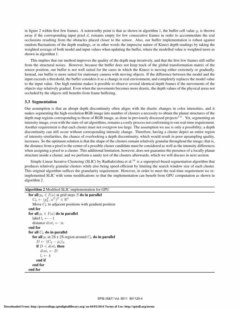
Simple Linear Iterative Clustering (SLIC) by Radhakrishna et al.10 is a superpixel-based segmentation algorithm that

produces relatively granular clusters while also being speed-efficient by limiting the search window size of each cluster.

This original algorithm suffices the granularity requirement. However, in order to meet the real-time requirement we re-

implemented SLIC with some modifications so that the implementation can benefit from GPU computation as shown in

algorithm 2.

Algorithm 2Modified SLIC implementation for GPU

for all pk ∈ I(u) at grid steps S do in parallel

Ck ← (pTk , uT )T ∈ R

5

Move Ck to adjacent positions with gradient position

end for

for all pi ∈ I(u) do in parallel

label li ← −1distance disti ←∞

end for

for all Ck do in parallel

for all pi in 2S x 2S region around Ck do in parallel

D ← ||Ck − pi||2if D < disti thendisti ← Dli ← k

end if

end for

end for

SPIE-IS&T/ Vol. 9011 901120-4


5, 0

.45.

1110111011111111tte...iti111111MISIIMMISW10/111111111111.1611"11111,041(411111111111111111111161WMFA1111111111111111111.4017111111111111111110111k1111111111111.1101,11"jd111111111011,0W111IMINIMP11461001011111111/0.0S 4,141111111111111i0V,;41% ¡".%

1111111111/1111 Pit-11mums* *fr,'lam limitntaltitfAcIIIIIIN4 kW1111111111111111111tAlltiMill111111111111/14.4411111111111101101111111"ir

111111111111111110111041,11111111111111111111111114041

11111111111111111110111101

1111111111111tOMMITIM111111111111101Or 41161-c.611

111111111111,11/.. '31411111111111111MV 4 IA4.4sanutafwwwww,t,moind , 4*

Otvialnummuna, 41 linmariffsoici.

Figure 3. GPU SLIC image segmentation. Left: input RGB image. Center: SLIC segmentation result for single iteration. Right:

SLIC segmentation result for 10 iterations. No visually distinguishable difference was produced by adding iterations. Single iteration

segmentation is used for further processing.

In order to maximize the throughput of GPU parallel computation, we parallelized not only the initial steps of the

segmentation by assigning threads to all pixels, but also the actual segmentation procedure by assigning multiple threads

per cluster so that the clusters grow more rapidly. However, special atomic instruction is used to avoid race condition that

happens when multiple threads attempt to assign a pixel to different clusters, therefore effectively serializing the control

flow. While such serialization is necessary to avoid excessive number of disjointed pixels resulting from the aforementioned

race conditions, it also decreases the throughput of the segmentation, therefore reducing the throughput. However, we

observed that the effect of decreased throughput becomes negligible if the number of clusters is kept sufficiently large,

which results in increased number of threads and consequently reducing the magnitude of overall serialization.

SLIC is originally a multi-pass segmentation algorithm that iterates until the clusters converge; however, we observed

that such iteration is too computationally heavy even with fully pipelined GPU implementation. Because the segmentation

result is to be used to partition the already-downsampled depth map, complex cluster edges are prone to get ignored. This

lead us to abandon the multi-pass nature of the original algorithm, and to only rely on the very first configurations of the

clusters. This also allows the removal of the related post-processing procedures of the original SLIC algorithm from our

implementation, and it resulted in greatly reduced runtime of the segmentation, while still producing relatively granular

clusters as shown in figure 3.

3.4 Plane fitting

Segmenting I(u)makes it possible to partitionG(u′), which is already calibrated to the RGB image coordinates, into same

number of clusters by taking the correspondences between the depth map pixels and those of segmented intensity image

by using the fact that u′ originates from downsampling u by a factor of two. By denoting the linear transformation from u′

to u as u← π(u′), we can relate the depth clustersDCk ⊂ G(u′) to the intensity clusters µk ⊂ I(u) as follows:

DCk = {gi ∈ G(u′)| pπ(i) ∈ µk ⊂ I(u)}. (2)

As previously stated, our assumption, as in many related works,1–4 is that the sharp depth discontinuities are likely to

align with those of intensity similarities. This implies that each depth map clusterDCk likely contains relatively continuous

surfaces, or possibly even a completely planar surface. This makes it possible to attempt fitting planar equations to each

depth cluster.

To fit a plane model to each cluster, first we obtain a vertex map,

V (u′) ⊂ R3 = D′(u′)K−1u̇′, (3)

whereK denotes a camera calibration matrix for Kinect depth sensor that performs transformation of coordinates between

camera and image coordinate systems, and u̇′ = (u′ | 1)T . V (u′) and G(u′) stores their elements vi and gi in same image

plane coordinate system u′, vertice clusters V Ck ⊂ V (u′) can be trivially defined as follows:

V Ck(u′) = DCk(u

′)K−1u̇′, (4)

SPIE-IS&T/ Vol. 9011 901120-5


and subsequently can be used for cluster-wise planar fitting.

There exist number of ways for fitting planar equations to a set of points in 3-dimensional space. Among all the most

frequently used is Random Sample Consensus(RANSAC) based approach, relying on randomization and iterations. How-

ever we found such method to be infeasible for real-time efficiency, in that the moment of convergence is too indeterministic

because of the random subsamplings.

Another method is Principal Conponent Analysis(PCA), used by many modern research projects including.11 By

building a covariance matrix of the population and concentrating the axis-wise variances to the first few dimensions of

the corresponding eigensystem, PCA is often used as dimension-reduction method. Because V Ck ⊂ R3, applying PCA

to each V Ck results in 3 x 3 covariance matrix. By exploiting that the eigenvectors are ordered in decreasing variance

representation of the population, we can assume that the last eigenvector of the covariance matrix represents the normal

vector of the optimal fitted plane, because it has the same direction of the cross product of the two vectors depicting the

two largest variance directions.

However, it is possible that some V Ck does not necessarily contain planar structures, as discussed in previous sections.

We therefore need to perform a sanity check of the fitted plane to avoid erroneously upsampling a complex non-planar

structure as a simplified planar representation. The eigenvalues associated with each eigenvector of the covariance matrix

obtained by performing PCA are proportional to the magnitude of the variance depicted by the corresponding eigenvectors.

This implies that if the corresponding eigenvalue of the last eigenvector is large, the first two eigenvectors are insufficient

in depicting all variances of the population. In other words, the population has three variance directions, indicating that it

is not a planar structure. Therefore, we can check the validity of the fitted plane just by looking at its eigenvalue, and if it is

larger than a threshold, the plane model is rejected. This makes the plane sanity check trivial enough to maintain real-time

performance.

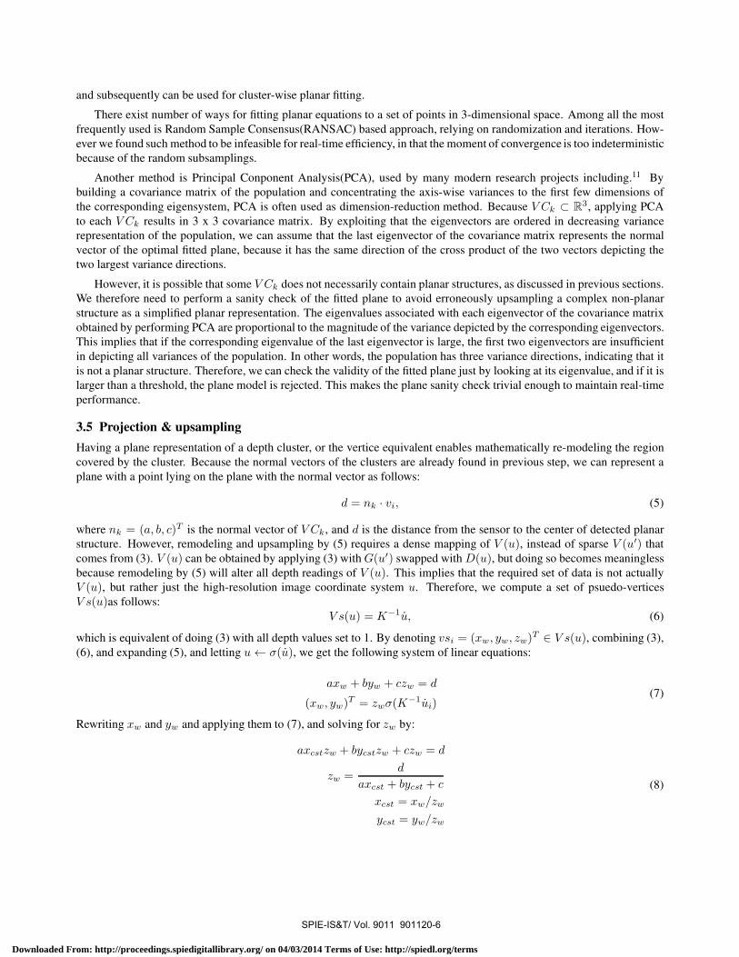
3.5 Projection & upsampling

Having a plane representation of a depth cluster, or the vertice equivalent enables mathematically re-modeling the region

covered by the cluster. Because the normal vectors of the clusters are already found in previous step, we can represent a

plane with a point lying on the plane with the normal vector as follows:

d = nk · vi, (5)

where nk = (a, b, c)T is the normal vector of V Ck , and d is the distance from the sensor to the center of detected planar

structure. However, remodeling and upsampling by (5) requires a dense mapping of V (u), instead of sparse V (u′) thatcomes from (3). V (u) can be obtained by applying (3) withG(u′) swapped withD(u), but doing so becomes meaningless

because remodeling by (5) will alter all depth readings of V (u). This implies that the required set of data is not actually

V (u), but rather just the high-resolution image coordinate system u. Therefore, we compute a set of psuedo-vertices

V s(u)as follows:V s(u) = K−1u̇, (6)

which is equivalent of doing (3) with all depth values set to 1. By denoting vsi = (xw, yw, zw)T ∈ V s(u), combining (3),

(6), and expanding (5), and letting u← σ(u̇), we get the following system of linear equations:

axw + byw + czw = d

(xw, yw)T = zwσ(K

−1u̇i)(7)

Rewriting xw and yw and applying them to (7), and solving for zw by:

axcstzw + bycstzw + czw = d

zw =d

axcst + bycst + c

xcst = xw/zw

ycst = yw/zw

(8)

SPIE-IS&T/ Vol. 9011 901120-6


7;-;-:;;i..7

,"1";'

;

-

- - .4;

f

- , . -* kV , , ' ' - o ,, '"Ii.L 'n'r.' -;''.'" ;,' ''',. '', 2...1.:','''..'

- ,I ."WI

ï t,_. t.,_

. 0 ' "

we get the re-modeled depth mapDup(u) = {zw} of dense population u. While this suffices the upsampling of G(u′), wefurther re-generate Vup(u),

Vup(u) = Dup(u)K−1u̇ (9)

to show that our approach can be used for generating stream of free-viewpoint images.

As discussed previously, not all clusters contain planar structures that can be upsampled as described. For such clusters,

which are already identified in plane-fitting phase of the pipeline, we instead useLIG(u) to prevent erroneous linearlizationof complex structures. Also, it is important to note that the steps described so far are all efficiently implemented in GPU to

gain from massively parallel computation.

4. PERFORMANCE

4.1 Experimental setting

Our full framework is implemented in a system equipped with i7-3940XM, GeForce 680M, and 32GB of memory. We

used OpenCV for trivial visualizations of color and depth images as well as data manipulations, and PointCloudLibrary for

3-dimensional visualization. Microsoft Kinect was accessed via Prime Sense drivers. All GPGPU implementations were

done with computing capability 2.0 of CUDA version 4.0.

4.2 Runtime

For any type of scenary captured by Kinect, we observed that our system is able to maintain high-frame rate, ranging

from 24 to 27. This fluctuations in processing time is resulting from the plane sanity check; because parts of Vup(u)are overwritten with LIG(u) according to the planar fitting quality, the amount of post-processing is proportional to the

complexity of the scene captured by Kinect. The distribution of the computational cost is presented in table 1.

Steps Computation cost[%]

Downsample 1.69

Frame accumulation 1.71

Interpolation 4.94

Segmentation 55.72

Plane fitting 30.0

Projection 3.61

Upsample 2.32Table 1. Computational cost for each step of the pipeline.

Figure 4. Left: Input RGB-D image in vertices form. Right: Upsampled depth image with corresponding colors in vertices form. Notice

that the the upsampled depth image has both interpolated and plane-based upsampled data

SPIE-IS&T/ Vol. 9011 901120-7


Figure 5. Magnified visualization of parts of figure 4 where planar structure is present. Upper: raw input, Bottom: upsampled result.

Notice the uniform distribution of the data. Also visible is the piecewise remodelings of the large surface.

4.3 Overall results

Having interpolated input image as a backup for plane-based upsampling implies that our system can always upsamples

for every downsampled pixel values of the original input depth image. As shown in figure 4, our system can reproduce the

dense depth data from the downsampled input depth with an extreme visual similarity.

Visual similarity between the upsampled image and the original input image also implies that our assumption of

intensity-depth discontinuity coincidence is valid; for total 240 clusters of the input RGB image, depending on the scene

complexity, from aroud 100 to as many as 220 clusters were identified to contain planar structures by performing the planar

model sanity checks.

Being able to compute planar structures of each cluster brings an additional benefit other than merely reproducing the

geometric structure. As discussed in earlier chapters, the raw depth readings fromKinect is often heavily contaminatedwith

structural noises. Moreover, because of the triangulation based on the projected pattern, smooth surfaces are represented in

discretized depth readings. However, remodeling based on the planar structures for upsampling is independent of the input

depth readings once the planar model has been found, we can completely replace the inevitably discretized representations

of smooth flat surface with true flat representation as shown in figure 5. This new uniformly dense representation of planar

structures is especially suited for free-viewpoint images, since they provide constant visualization unlike the descritized

stepwise readings of raw Kinect depth map. However, a large planar structure can be represented as a series of smaller

planar structures as shown in figure 5. This is due to the fact that the planar fitting is done for piece-wise planar structures

depicted from RGB image segmentation. As stated however, it is not always feasible to fit a planar model to a cluster,

SPIE-IS&T/ Vol. 9011 901120-8


Figure 6. Example of complex and noisy subsection of depth structures. Up: Raw input RGB-D data in vertices form. Down: Cor-

responding upsampled depth data in RGB-D vertices form. Only the right and middle side of the upsampled data are based on planar

model fitting because of the spread of the input data is too 3-dimensional. Notice how the bottom left corner of the upsampled data

remains noisy and unevenly spread. Also, it is shown that the input image suffers from the discretization of smooth surface.

as shown in figure . Resulting from either absence of clearly depth edges, or depth-color edge misalignment, non-planar

clusters becomes drastically incorrect set of points when the planar fitting method is forcefully used. In such cases instead

LIG(u) is used in place of planar remodeling, which suffers from the same discontinuity problem present in the raw

readings. Also as visible in figure 6, the boundaries between LIG(u) and planar models do not go smooth, and can stand

out upon a careful inspection of the overall upsampled output.

Apart from visual assessments, we also conducted numerical analysis of the produced outcome of the system. Because

our assumed usage scenario is in real-time transmission, it is necessary to measure how well the output of our pipeline

resembles the input data. We observed the changes in the resulting upsampled depth map, in vertice form, to analyze the

different effects of changing the number of clusters, the strength of planar sanity check threshold, against three different

types of data coming from complex and simple geometric environments, as shown in figure 7. In order to assess the effect

of the alterations of parameters, the standard deviation of the resulting upsampled data is taken against the raw input data

for various settings of cluster numbers and threshold settings. The results are shown in the table 2.

Overall, it was observed that increasing the number of clusters tends to decrease the discrepancy between input and

output data for scenes 01 and 02. For scene 03, only when the planar fitting threshold is set loosely configured. This

phenomenon is determined to be resulting from the viewpoint of the Kinect when the experiment was performed for

SPIE-IS&T/ Vol. 9011 901120-9


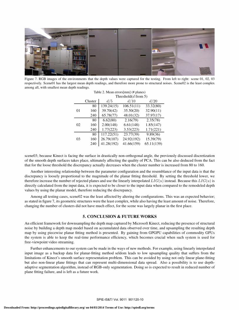
Figure 7. RGB images of the environments that the depth values were captured for the testing. From left to right: scene 01, 02, 03

respectively. Scene01 has the largest mean depth readings, and therefore more prone to structural noises. Scene02 is the least complex

among all, with smallest mean depth readings.

Table 2. Mean errors[mm] (# planes)

Threshold(d from 5)

Cluster d/5 d/10 d/2080 139.24(15) 106.51(11) 33.32(80)

01 160 39.70(42) 35.50(20) 32.90(11)

240 65.78(77) 48.01(32) 37.97(17)

80 6.62(80) 2.16(79) 2.35(78)

02 160 2.00(148) 6.61(148) 1.85(147)

240 1.77(223) 3.53(223) 1.71(221)

80 117.22(51) 23.77(39) 9.89(36)

03 160 26.79(107) 24.92(192) 15.39(79)

240 41.28(192) 41.66(159) 65.11(139)

scene03; because Kinect is facing the surface in drastically non-orthogonal angle, the previously discussed discretization

of the smooth depth surfaces takes place, ultimately affecting the quality of PCA. This can be also deduced from the fact

that for the loose threshold the discrepancy actually decreases when the cluster number is increased from 80 to 160.

Another interesting relationship between the parameter configuration and the resemblance of the input data is that the

discrepancy is loosely proportional to the magnitude of the planar fitting threshold. By setting the threshold lower, we

therefore increase the number of rejected planes and use the linearly interpolatedLIG(u) instead. Because this LIG(u) isdirectly calculated from the input data, it is expected to be closer to the input data when compared to the remodeled depth

values by using the planar model, therefore reducing the discrepancy.

Among all testing cases, scene02 was the least affected by altering the configurations. This was an expected behavior;

as stated in figure 7, its geometric structures were the least complex, while also having the least amount of noise. Therefore,

changing the number of clusters did not have much effect, for the scene was largely planar in the first place.

5. CONCLUSION& FUTUREWORKS

An efficient framework for downsampling the depth map captured by Microsoft Kinect, reducing the presence of structural

noise by building a depth map model based on accumulated data observed over time, and upsampling the resulting depth

map by using piecewise planar fitting method is presented. By gaining from GPGPU capabilities of commodity GPUs

the system is able to keep the real-time performance efficiency, which becomes crucial when such system is used for

free-viewpoint video streaming.

Further enhancements to our system can be made in the ways of new methods. For example, using linearly interpolated

input image as a backup data for planar-fitting method seldom leads to low upsampling quality that suffers from the

limitations of Kinect’s smooth surface representation problem. This can be avoided by using not only linear plane-fitting

but also non-linear plane fittings that can represent multi-dimensional data spread. Also a possibility is to use depth-

adaptive segmentation algorithm, instead of RGB-only segmentation. Doing so is expected to result in reduced number of

plane fitting failure, and is left as a future work.

SPIE-IS&T/ Vol. 9011 901120-10


ACKNOWLEDGEMENT

This work is partially supported by National Institute of Information and Communications Technology (NICT), Japan.

REFERENCES

[1] J. Kopf, M. F. Cohen, D. Lischinski, and M. Uyttendaele, “Joint bilateral upsampling,” ACM Transactions on Graph-

ics 26(3), p. 96, 2007.

[2] Y. Li and L. Sun, “A novel upsampling scheme for depth map compression in 3DTV system," in Picture CodingSymposium (PCS), 2010, pp. 186–189, IEEE, 2010.

[3] D. Chan, H. Buisman, C. Theobalt, S. Thrun, et al., “A noise-aware filter for real-time depth upsampling,” in Work-

shop on Multi-camera and Multi-modal Sensor Fusion Algorithms and Applications-M2SFA2 2008, 2008.

[4] M. Wildeboer, T. Yendo, M. P. Tehrani, T. Fujii, and M. Tanimoto, “Color based depth up-sampling for depth com-

pression,” in Picture Coding Symposium (PCS), 2010, pp. 170–173, IEEE, 2010.

[5] Y. Soh, J.-Y. Sim, C.-S. Kim, and S.-U. Lee, “Superpixel-based depth image super-resolution,” in IS&T/SPIE Elec-

tronic Imaging, pp. 1–10, International Society for Optics and Photonics, 2012.

[6] J. Diebel and S. Thrun, “An application of markov random fields to range sensing,” Advances in neural information

processing systems 18, p. 291, 2006.

[7] X. Xiang, G. Li, J. Tong, M. Zhang, and Z. Pan, “Real-time spatial and depth upsampling for range data,” Transactions

on computational science XII , pp. 78–97, 2011.

[8] S. Holzer, R. Rusu, M. Dixon, S. Gedikli, and N. Navab, “Adaptive neighborhood selection for real-time surface

normal estimation from organized point cloud data using integral images,” in IEEE/RSJ International Conference on

Intelligent Robots and Systems (IROS), pp. 2684–2689, IEEE, 2012.

[9] R. A. Newcombe, A. J. Davison, S. Izadi, P. Kohli, O. Hilliges, J. Shotton, D. Molyneaux, S. Hodges, D. Kim, and

A. Fitzgibbon, “Kinectfusion: Real-time dense surface mapping and tracking,” in 10th IEEE International Symposium

on Mixed and Augmented Reality (ISMAR), pp. 127–136, IEEE, 2011.

[10] R. Achanta, A. Shaji, K. Smith, A. Lucchi, P. Fua, and S. Susstrunk, “Slic superpixels compared to state-of-the-art

superpixel methods,” in IEEE Transactions on Pattern Analysis and Machine Intelligence, pp. 2274–2282, IEEE,

2012.

[11] T. Hayashi, F. de Sorbier, and H. Saito, “Texture overlay onto non-rigid surface using commodity depth camera.,” in

VISAPP, pp. 66–71, 2012.

SPIE-IS&T/ Vol. 9011 901120-11


joint upsampling and noise reduction fo r real-time depth

Documents