jointly periodic points in cellular automata - school of computer

JOINTLY PERIODIC POINTS IN CELLULAR AUTOMATA

MIKE BOYLE AND BRYANT LEE

Abstract. For a one-dimensional surjective cellular automaton, we consider

temporal periodicity of spatially periodic points. We offer some questions,

facts and experimental results.

Contents

1. Introduction 12. Definitions and background 23. Some mechanisms for periodicity 44. Experimental results 65. Discussion of the computer program 76. Tables 8References 23

1. Introduction

In this paper we consider the action of a surjective one-dimensional cellular au-tomaton map f on spatially periodic points. (In the language of symbolic dynamics[9, 11, 13]), f is a surjective endomorphism of SN , the full shift on N symbols, whereN is the size of the symbol set of the automaton.) This paper is primarily an ex-perimental mathematics paper, based on data from a computer program written byauthor Lee. The experimental results and mathematical context, which we explain,lead us to questions and a conjecture on the growth rate of the spatially periodicpoints which are also temporally periodic points.

To express the questions and conjecture, we make the following definitions. LetPk(S) denote the points of period k of S, i.e. the points fixed by Sk, and letPer(S) = ∪kPk(S). So, Per(SN ) is the set of spatially periodic points for a one-dimensional cellular automaton on N symbols. Let νk(f, SN ) denote the numberof jointly periodic points in Pk(S) (i.e. points periodic under f as well as SN ), anddefine

ν(f, SN ) = lim supk

νk(f, SN )1/k .

These definitions make sense for any f commuting with any SN : X → X.

Question 1.1. Is it true for every surjective one-dimensional cellular automatonf on N symbols that ν(f, SN ) ≥

√N?

2000 Mathematics Subject Classification. 37B10.Key words and phrases. cellular automaton; shift of finite type; periodic points.Partially supported by NSF Grant 0400493 and NSF VIGRE Grant xxx.

1

2 MIKE BOYLE AND BRYANT LEE

Question 1.2. Is it true for every surjective one-dimensional cellular automatonf on N symbols that ν(f, SN ) > 1?

Conjecture 1.3. There exists N > 1 and a surjective cellular automaton f on Nsymbols such that ν(f, SN ) < N

In Section 2, we give detailed definitions and background. In Section 3, we de-scribe some mechanisms by which one can prove lower bounds for ν(f, SN ) for somef , and discuss the questions. In Section 4, we discuss the experimental evidence(which is collected in tables at the end). In Section 5, we discuss the computerprogram we use. We collect the data tables in Section 6.

2. Definitions and background

In this section we recall some background. For a thorough introduction to thesetopics, see [11] or [13].

Let A be a finite set of N elements (the symbol set), with the discrete topology.Let ΣN be the product space AZ, with the product topology. We view a point x inΣn as a doubly infinite sequence of symbols from S, so x = . . . x−1x0x1 . . . . Thespace ΣN is compact metrizable, and one metric compatible with the topology isdist(x, y) = 1/(|n| + 1) where |n| is the minimum nonnegative integer such thatxn 6= yn. A set E is dense in ΣN in this topology if for every k and every word Win A2k+1 there exists x in E such that x[−k, k] = W .

The shift map σ : Σn → Σn is the homeomorphism defined by the rule (σx)i =xi+1. The topological dynamical system (ΣN , σ) is called the full shift on n symbols.If X is a closed shift-invariant subsystem of some full shift, then (X,σ|X) is asubshift. If X is exactly the subsystem of points which never see some given finiteset of words, then (X,σ|X) is a shift of finite type. These subshifts are useful andnatural for the study of cellular automata (see the remarks in [4]). For a lighternotation, we may sometimes use a single letter like S to represent a subshift (X,σ|X)or the restricted shift map σ|X .

The entropy h(S) of a subshift S = (X,σ|X) is the growth rate of S-words:h(S) = limk(1/k) log(|{x[1, k] : x ∈ X|}). In particular, h(SN ) = logN .

A map f : ΣN → ΣN is a continuous and shift-commuting (fσ = σf) if and onlyf is a block code, i.e. there exist integers a, b and a function F : Ab−a+1 → A suchthat (fx)i = F (x[i + a, i + b]) for all integers i and all x ∈ ΣN . Such a map f iscalled a one-dimensional cellular automaton map. If b−a+1 is minimal for f , thenit is the span of f . There is a well known dichotomy for such maps f : either (i) fis surjective and for some integer M every point has at most M preimages, or (ii)image points typically have uncountably many preimages, and f is not surjective[9, 11, 13]. For an onto c.a. map f , there is a positive integer d, the degree of f ,such that most points have d preimage points under f , and no point has fewer thand preimage points.

We restrict our attention to surjective maps in this paper because we are inter-ested in periodic points of f , which must be contained in ∩k>0f

kΣN , the eventualimage of f . We separate our ignorance about periodic points from additional diffi-culties involving the passage to the eventual image [14].

If N is prime, then every c.a. map f on N symbols can be presented by a uniquepolynomial [9] over the finite field Z/N . For example, x−1 + x1x2 defines the c.a.map f such that for all x, (fx)i = xi−1 +xi+1xi+2. (If N is not prime, there is still

PERIODIC POINTS 3

a representation by products of polynomials over suitable finite fields [15], whichwe won’t need.) If (fx)0 is determined by x[a, b], with a maximal and b minimal,then b − a + 1 is the span of f . If a is not specified, then it is assumed a = 0.A c.a. map on SN can also be defined by a lookup code, as in tables 8 and 9.For example, with N = 2, order the 23 words on symbols {0, 1} lexicographically(000,001,010,011,100,101,110,111); then the lookup code for a span 3 c.a. f is givenby the word c1c2 . . . c8 on {0, 1} such that (fx)0 = ci if x0x1x2 is the ith word inlexicographic order. E.g., x0 + x1x2 corresponds to lookup code 00011110.

A block code f : ΣN → ΣN is right-closing if it never collapses distinct left-asymptotic points. This means that if f(x) = f(x′) and for some I it holds thatxi = x′i for −∞ < i ≤ I, then x = x′. The definition of left closing is given byreversing the inequality. The map f is closing if it is either left or right closing. Aclosing c.a. map is surjective. An endomorphism of a full shift SN is constant-to-oneif and only if it is both right and left closing.

If f is given by a polynomial which is linear in the leftmost variable (e.g. x−1+x1x2), then f is left closing. If a map is linear in the leftmost variable xi, withi = 0, then f is called left permutative. If f is linear in the rightmost variable, thenf is called right permutative, and f is right closing.

Closing maps are important in the coding theory of symbolic dynamics [11,13]. The immediate relation to the current paper is the following fact: if f is aclosing one-dimensional cellular automaton map, then the jointly periodic pointsin the cellular automaton are dense [4]. It is an open question as to whetherevery surjective cellular automaton map has dense periodic points. This is a goodexample of the difficulty of resolving the most basic questions about periodic pointsand cellular automata.

There are many onto c.a. maps. Let ak, bk, ck be the number of span k c.a. mapson SN which are respectively injective, surjective, arbitrary (so, ck = NNk

). If dk isany of the quantities ak, bk, ck, ck/bk, bk/ak, then limk(1/k) log log dk = logN (fordk = ak this was proved in [10]; quantitative estimates related to the rest were toour knowledge first written in an unpublished manuscript of Milnor FIND REF-ERENCE. There are more constructive abundance results: many automorphismsof subsystems extend to automorphisms of SN [6], and closing maps of subsystemsextend to closing maps of SN [1].

Given a map g, we let Fix(g) or Pk(g) denote the set of fixed points of gk.E.g., Fix(SN ) = Nk. We let P o

k (g) denote the points of least period k of g. E.g.,P o

3 (S2) = 8− 2 = 6. Pk(SN ) is mapped into itself by any c.a. f . We define

νk(f, SN ) = |{x ∈ Pk(SN ) : ∃j > 0, f jx = x}| , ν(f, SN ) = lim supk

νk(f, SN )1/k ,

νok(f, SN ) = |{x ∈ P o

k (SN ) : ∃j > 0, f jx = x}| , ν(f, SN ) = lim supk

νok(f, SN )1/k .

For a c.a. map f of SN , the jointly periodic points are those which are both f -periodic (temporally periodic) and SN -periodic (spatially periodic). We record aremark indicating the subtlety of the periodic behavior of the jointly periodic points.

Remark 2.1. Suppose φ and ψ are automorphisms of SN and N is prime. Possiblyafter replacing φ, ψ with φSj , ψS` for some integers j, `, there will exist a κ > 0such that

|Fix(Smφn)| = |Fix(Smψn)| = |Fix(Sm)|


whenever 0 < |m/n| < κ [5]. At the same time, the sequences (|Fix(φn)|) and(|Fix(ψn)|) can be very different. A dramatic example of this sort in the setting ofshifts of finite type is part of [16, Example 10.1].

Remark 2.2. Suppose x ∈ Per(SN ) and f is an endomorphism of SN = S. Then xis in Per(f) if and only if for some i > 0, f ix and x are in the same S-orbit. Thusfor all integers i, j, k,m with m, i, k positive, we have νk(f, S) = νk(f iSj , Sm), andconsequently ν(f, S) = ν(f iSj , Sm).

3. Some mechanisms for periodicity

Throughout this section f denotes a c.a. map on N symbols. In this section, wediscuss four ways to demonstrate ν(f, SN ) is large:

(1) find a large shift fixed by f (or more generally by a power of f)(2) let f be a group endomorphism(3) use the algebra of a polynomial presenting f(4) find equicontinuity points.

After discussing these, we offer a random maps heuristic and a question.We will exhibit the first mechanism in some generality. We prove Proposition

3.2 below to show that there is no property of f considered just as a quotient map(i.e., a map between systems which is not iterated) which prevents ν(f, SN ) frombeing arbitrarily close to N . To avoid a digression into detailed symbolic dynamics,we only outline the proof of the technical lemma we need for this result. Below,e.g. fφ denotes the composition f ◦ φ, i.e. φ followed by f .

Lemma 3.1. Suppose S is a mixing SFT, and f : S → S is a surjective block code,and ε > 0. Then there is an automorphism φ of (XA, S) and a shift of finite typeT contained in S such that h(T ) > h(S)− ε and the fixed point set of φf containsT .

Outline of proof. First, using magic words [11, 13] construct an SFT T1 in S suchthat h(T1) > h(S) − ε/2 and the restriction of f to T1 is injective. Then pick Msuch that for every n ≥ M , S has at least two orbits of length n which are notin T1. Then choose T to be an SFT inside T1 such that T has no orbits of lengthsmaller than M and also such that h(T ) > h(S) − ε. Now the image of T is anSFT T ′ isomorphic to T , and there is a block code g : T ′ → T such that on T , gfis the identity map. By [6, Theorem 1.5], there is an automorphism φ of S whoserestriction to T ′ equals g. Clearly the restriction of φf to T is the identity map. �

Proposition 3.2. Suppose f is a surjective c.a. on N symbols and ε > 0. Thenthere is an invertible c.a. φ such that log(ν(φf, SN ) > h(SN )− ε.

Proof. If T is a shift of finite type, then lim supk(1/k) log |Fix(T k)| = h(T ). Givenf , choose φ and T as in Lemma 3.1, then νk(fφ, SN ) ≥ |Fix(T k)|. Consequentlylog(ν(φf), SN )) ≥ log(N)− ε = h(SN )− ε. �

Remark 3.3. The statements of Lemma 3.1 and Proposition 3.2 remain true if φfis replaced by fφ. One way to see this is to notice that the systems (fφ, S) and(φ(fφ)φ−1, φSφ−1) = (φf, S) are isomorphic.

PERIODIC POINTS 5

Now we turn to algebra. The points of SN form a group under coordinatewiseaddition (mod N), and some c.a. are endomorphisms of this group; in the terminol-ogy of [15], these c.a. are linear. Such maps are given by nonconstant polynomialswhich are sums of monomials.

Proposition 3.4. Suppose a surjective c.a. map f is linear on SN . Then for alllarge primes p, νp(f, SN ) ≥ Np−1. Therefore ν(f, SN ) = N .

Proof. We use an argument from the proof of a related result [4, Proposition 3.2].Let M be the cardinality of the kernel of f . Suppose p > M and p is prime;then f must map orbits of length p to orbits of length p (otherwise, some orbit oflength p would be collapsed to an orbit of length dividing p, i.e. to a fixed point,which would contradict the fact that every point has M preimages, with M < p).Therefore, for all k, the kernel of fk contains no point in an orbit of length p. Thefixed points of (SN )p form a subgroup H which is mapped into itself by f , so forsome k > 0, the restriction of fk to fkH is injective, and all points in the set fkHare f -periodic. Because the kernel of (fk)|H contains at most N points, it followsthat at least 1/N of the fixed points of Sp are periodic for f . �

In the linear case, the algebraic structure allows a number theoretic descriptionof the way that f -periods of jointly periodic points of SN period k vary (quiteirregularly) with k [15]. In the nonlinear case we have nothing close to such anunderstanding.

Algebra can be used in a different way. Again, cellular automata maps can bepresented by polynomials [9, 15]. Frank Rhodes [18] used algebraic properties ofthese to exhibit a family of one-dimensional noninjective c.a. such that νo

k(f, SN ) =|P o

k (SN )| for all k outside mN, where m is a positive integer greater than 1. Clearlyin this case ν(f, SN ) = N . We will not review that argument.

We now turn to equicontinuity. A point x is equicontinuous for f if there arepositive integers K,M such that for all points y, if x[−K,K] = y[−K,K] then forall n > 0 (fnx)[−M,M ] = (fny)[−M,M ]. If the surjective c.a. f has a point ofequicontinuity, then limn(1/n) log νn(f, SN ) = log(N) [2]. Points of equicontinuityoccur in various natural examples (e.g. [3, 12]).

For most surjective c.a., the criteria above are not applicable. This leads tothe experimental investigations discussed in the next section, and to the possibilityraised in Questions 1.1 and 1.2 of a general plenitude of spatially periodic points.Question 1.1 arises because in the experimental data, the restrictions of the c.a.f to Pk(SN ) are somewhat reminiscent of a random map on a finite set. Sincef is a surjective c.a. map, there is an M such that no point has more than Mpreimages under f . Suppose for example k is a prime greater than M and letOk(SN ) denote the set of Sn orbits of size N . Then f defines an at most M -to-1map fk from Ok(SN ) into itself, and it is perhaps a plausible heuristic that, in theabsence of some additional structure, members of the sequence (fk) will displaysome of the behavior of random maps; and that “additional structure” such asexistence of equicontinuity points may serve to put a floor rather than a ceilingon the numbers νk(f, SN ). The beautiful and extensive theory of random mapson finite sets provides precise asymptotic distributions answering various naturalquestions [19]. Here we simply note that for a random map on a set of K elements:asymptotically on the order of

√K of the elements will lie in cycles (whether the


map is bounded-to-one as in [7, Theorem 2], or not [19]); the longest cycle will beon the order of

√K; and there will be few big cycles.

The maps fk, derived from the surjective c.a. f , do have one other obviousnonrandom property [9, 11, 13]: most points have the minimal possible number ofpreimages. This does not work against the heuristic behind Question 1.1.

We cannot answer Question 1.2 even in the case where f is a “closing” mapand we know there is an abundance of jointly periodic points [4]. Conjecture 1.3is a stronger expression of our ignorance. From the experimental data discussedbelow, it seems clear that there will be many surjective c.a. f with ν(f, SN ) < N .However, we cannot give a proof for any example.

4. Experimental results

With two exceptions, f below is a surjective c.a. defined on the full shift SN withN = 2, with symbol set {0, 1}. The two exceptions are Tables 18 and 19, whereN = 3. In the tables which display individual maps, in row k counts are made fromthe Nk points of (not necessarily least) shift period k. P denotes the number ofpoints of which are also periodic under f , and L denotes the number of points inthe largest f -cycle. The preperiod of a point x is the smallest nonnegative integerj such that f j(x) is f -periodic. The period of a point is the size of the f -cycleinto which it moves under the action of f . Note that the data for P 1/k and L1/k isperhaps suggestive of a common limsup of at least

√N .

The computer program gives more information than this; it will list the lengthsand multiplicities of all f -cycles, and all f -preperiods. We have suppressed most ofthis (which can be found at Boyle’s web site) for reasons of space.

Example 4.1. [A linear map] In Table 1, we exhibit the output for a familiar exam-ple, the map f defined by the rule f(x)[0] = x[0] + x[1] (where addition is mod 2).This map is linear (a group endomorphism) and everywhere 2-to-1.

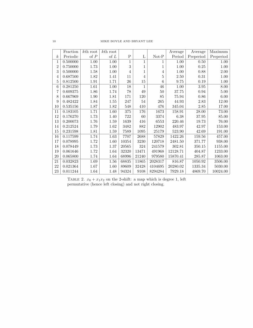
Example 4.2. [Permutative] In Table 2, we exhibit results for x0 +x1x2, a degree 1map which is not right closing but which is left permutative and hence left closing.

Example 4.3. [Not closing] In Table 3, we consider a map which is neither leftclosing nor right closing. The map is constructed by composing a not-left-closingmap and a not-right-closing map.

Example 4.4. [2-to-1 linear composed with degree 1 closing ] In Table 4, the c.a.map is a composition, the linear degree two map x0 + x1 followed by a degree oneleft permutative (hence left closing) map.

Example 4.5. [Linear composed with automorphism] In Table 5, we exhibit resultsfor a biclosing map which is not linear in the end variables. For this, we simplycompose the map of Example 4.1 with an involution (an automorphism U such thatU2 is the identity map). The immediately striking feature is that this compositiondrastically reduces the sequence (νn) in comparison with Example 4.1.

Example 4.6. [Bipermutative] In Table 6, we exhibit results for the nonlinear mapx−1 + x0x1 + x2, which is however linear in both end variables. The results don’tseem all that different from the biclosing example 4.5 above.

Example 4.7. [Closing] In Table 7, we exhibit results for a left closing map whichis not right closing and is not linear in the leftmost variable. This map is thecomposition of the left permutative map of Table 2 with an involution.

PERIODIC POINTS 7

Hedlund, Appel and Welch conducted an early investigation [8] in which theyfound all surjective c.a. on two symbols of span at most five. (This was not trivial,especially in 1963, because there are 232 c.a. maps of span at most five.) Among allonto maps of span at most four, there are exactly 32 which are not linear in an endvariable and which send the point . . . 0000 . . . to itself. There are listed in Table8. Any other span four onto map which is not linear in an end variable is one ofthese 32 maps g precomposed or postcomposed with the flip map F (given by thepolynomial x0 +1). Because gF = F (Fg)F = F−1(Fg)F , the jointly periodic datafor Fg and gF will be the same. We exhibit νo

k(·, S2) in Tables 10 – 13 for the 32maps g and the 32 maps Fg. (νo

k(·, S2) counts out of points of least shift period kwhile νk(·, S2) counts out of points of (not necessarily least) shift period k.)

According to [8], there are 141,792 surjective c.a. maps of span 5. These arearranged in [8] into classes – linear in end variables, compositions of lower-spanmaps, remainder. The remainder class (11,388 maps) is broken down into subclassesby patterns of generation, and a less regular residual class of 200 maps. The residualclass is generated with various operations by the 26 maps we copy in Table 9 from[8, Table XII]. As some kind of sample, in Tables 14 and 15 we display νk(·, S2)(k ≤ 19) for these 26 maps of span 5.

In Table 16, we generate a sample of 16 span 5 resolving maps as follows.Let pn(x[0, 4]) denote the polynomial rule map for map n in Table 16 and letqn(x0, x1, x2, x3) denote the polynomial rule for the map n in Table 8. Then pn isdefined by pn = x0 + qn(x1, x2, x3, x4). The purpose of Table 16 is to make a roughcomparison of a sample of maps which are and are not linear in an end variable.We see no particular difference.

In Table 17 we give a composition of an arbitrarily chosen pair of span 4 ontomaps. The decay in νk with k is similar to to that in the previous tables.

Finally, in Tables 18 and 19 we look at two examples on the 3-shift. We can’tfor computer memory reasons look at orbits of long shift period.

5. Discussion of the computer program

Our data come from the program FPeriod developed by author Lee. FPeriodtakes as input N , the number of symbols in the shift; k, the shift period of thepoints; and F , the function that induces the block code f . It tests all points thatare shift periodic of period k and determines how many are f -periodic, as well aslisting the multiplicity of points for each f -period, the multiplicity of orbits andtheir periods, and the multiplicity of preperiods for the non-periodic points.

The algorithm. The points x of (not necessarily least) period k are in bijectivecorrespondence with the words x[0, k − 1]. The program computes (fx)[0, k − 1]from x[0, k − 1] using the rule F . The main idea of the underlying algorithm is tostart with a word of length k and continuously apply f , storing the generated pointsin a list, until some point is encountered twice. Then, the period and preperiod ofall the points in the list are known. Store all the points from the list, with theirperiod and preperiod information, in a table. Then, starting from the next pointnot in the table, continuously apply f and store the generated points until one oftwo conditions is met. Either some point is encountered twice, allowing the periodsand preperiods for the new points to be calculated, or some point already in thetable is encountered, in which case that point’s period and preperiod information


can likewise be used to calculate the periods and preperiods for the new points.Continue until the period and preperiod for all points of period k are found.

Algorithm complexity. The number of add-to-table, find-in-table, and evaluate-f operations is proportional to Nk. Thus, the time required by the algorithmis proportional to Nk. The add-to-table and find-in-table operations take timeproportional to a small constant, so the time taken by the evaluate-f operationsdominates the time of the overall algorithm. The memory required by the algorithmis also proportional to Nk because Nk points are eventually stored in the table.

The FPeriod program. FPeriod is a program written in the C++ programminglanguage that implements the algorithm given above. (An earlier Java version ranmuch more slowly.) It runs under Unix and related operating systems. It and itssource code are freely available under the GNU General Public License and canbe downloaded at http://www.math.umd.edu/∼mmb/. The more detailed outputfrom which the tables of the current paper were taken are also available there.

The program uses exponential amounts of time and memory, as per the algo-rithm, but in practice memory is the limiting factor. The program is quite fastbecause the f -evaluation operation is done by lookup tables. Although the usermay input the polynomial that induces f as a formula, the formula is convertedinto a table so it is faster to evaluate. Functions are only evaluated through actualcomputation if they are too large to store in a table.

The amount of memory used by the program limits the size of N and k thatcan be used. By nature of the algorithm, storing Nk points cannot be avoidedbecause it is necessary to remember which points were previously processed. Also,the storage of period and preperiod information for previously processed points iswhat allows new period and preperiod information to be derived quickly.

FPeriod uses 16 bytes of memory for each point stored in the table. An additionalseveral bytes per point are used by the table itself and by the dynamic memoryallocation system. In practice, running the program using N = 2 and k = 26required 1.8 gigabytes (1.8 billion bytes) of memory, close to the limit of a high-end computer. Note that this is more than (16 bytes) x (226) = 1.1 gigabytesand less than (32 bytes) x (226) = 2.1 gigabytes, which was reasonable to expect.Exponential memory use is inherent in the algorithm, and it is not feasible toimprove the memory use of the FPeriod program or a similar program enough toallow exploring significantly larger N or k values.

Additional features of the program include the ability to induce block codes fromcompositions of functions; the ability to separately track period and preperiod datafor points of least period k; and a truncated version which produces just output forνo

k .The FPeriod program was originally developed to produce experimental evidence

relevant to the open question of whether a surjective c.a. map must have denseperiodic points.

6. Tables

PERIODIC POINTS 9

Fraction kth root kth root Average Average Maximumk Periodic of P of L P L Not-P Period Preperiod Preperiod1 0.500000 1.00 1.00 1 1 1 1.00 0.50 12 0.250000 1.00 1.00 1 1 3 1.00 1.25 23 0.500000 1.58 1.44 4 3 4 2.50 0.50 14 0.062500 1.00 1.00 1 1 15 1.00 3.06 45 0.500000 1.74 1.71 16 15 16 14.12 0.50 16 0.250000 1.58 1.34 16 6 48 5.12 1.25 27 0.500000 1.81 1.32 64 7 64 6.91 0.50 18 0.003906 1.00 1.00 1 1 255 1.00 7.00 89 0.500000 1.85 1.58 256 63 256 62.05 0.50 1

10 0.250000 1.74 1.40 256 30 768 29.01 1.25 211 0.500000 1.87 1.69 1,024 341 1024 340.67 0.50 112 0.062500 1.58 1.23 256 12 3840 11.57 3.06 413 0.500000 1.89 1.67 4,096 819 4096 818.80 0.50 114 0.250000 1.81 1.20 4,096 14 12,288 13.89 1.25 215 0.500000 1.90 1.19 16,384 15 16,384 14.99 0.50 116 0.000015 1.00 1.00 1 1 65535 1.00 15.00 1617 0.500000 1.92 1.38 65,536 255 65,536 254.33 0.50 118 0.250000 1.85 1.30 65,536 126 196,608 125.73 1.25 219 0.500000 1.92 1.62 262,144 9,709 262,144 9708.96 0.50 120 0.062500 1.74 1.22 65,536 60 983,040 59.88 3.06 421 0.500000 1.93 1.21 1,048,576 63 1,048,576 62.99 0.50 122 0.250000 1.87 1.34 1,048,576 682 3,145,728 681.67 1.25 223 0.500000 1.94 1.39 4,194,304 2,047 4,194,304 2047.00 0.50 1

Table 1. x0 + x1 on the 2-shift: an algebraic, two-to-one map.


Fraction kth root kth root Average Average Maximumk Periodic of P of L P L Not-P Period Preperiod Preperiod1 0.500000 1.00 1.00 1 1 1 1.00 0.50 1.002 0.750000 1.73 1.00 3 1 1 1.00 0.25 1.003 0.500000 1.58 1.00 4 1 4 1.00 0.88 2.004 0.687500 1.82 1.41 11 4 5 2.50 0.31 1.005 0.812500 1.91 1.71 26 15 6 9.75 0.19 1.006 0.281250 1.61 1.00 18 1 46 1.00 3.95 8.007 0.609375 1.86 1.74 78 49 50 37.75 0.94 5.008 0.667969 1.90 1.81 171 120 85 75.94 0.86 6.009 0.482422 1.84 1.55 247 54 265 44.93 2.83 12.00

10 0.535156 1.87 1.82 548 410 476 345.04 2.85 17.0011 0.183105 1.71 1.60 375 176 1673 158.91 28.00 73.0012 0.176270 1.73 1.40 722 60 3374 6.38 37.95 85.0013 0.200073 1.76 1.59 1639 416 6553 220.46 19.73 76.0014 0.212524 1.79 1.62 3482 882 12902 483.97 42.97 153.0015 0.231598 1.81 1.59 7589 1095 25179 523.90 42.69 191.0016 0.117599 1.74 1.63 7707 2688 57829 1422.26 159.56 457.0017 0.078995 1.72 1.60 10354 3230 120718 2481.50 371.77 938.0018 0.078449 1.73 1.37 20565 324 241579 302.81 350.15 1155.0019 0.061646 1.72 1.64 32320 13471 491968 12128.71 404.87 1233.0020 0.065800 1.74 1.64 68996 21240 979580 15870.41 285.87 1063.0021 0.032823 1.69 1.56 68835 11865 2028317 816.87 1050.92 3506.0022 0.021364 1.67 1.60 89609 32428 4104695 20280.02 1335.34 5030.0023 0.011244 1.64 1.48 94324 9108 8294284 7929.18 4869.70 10024.00

Table 2. x0 + x1x2 on the 2-shift: a map which is degree 1, leftpermutative (hence left closing) and not right closing.

PERIODIC POINTS 11


10 0.261 1.74 1.49 268 55 756 20.18 6.75 1811 0.387 1.83 1.57 793 143 1255 53.53 3.00 1312 0.088 1.63 1.16 362 6 3734 1.39 20.61 4813 0.150 1.72 1.63 1236 611 6956 259.75 20.15 7814 0.126 1.72 1.51 2068 329 14316 119.61 33.22 13215 0.091 1.70 1.50 3014 465 29754 414.94 44.45 13816 0.092 1.72 1.50 6043 728 59493 650.33 101.66 28217 0.107 1.75 1.68 14145 6783 116927 3918.82 48.16 19618 0.060 1.71 1.58 15753 4095 246391 3406.78 110.78 39619 0.072 1.74 1.60 38191 7619 486097 6336.19 142.98 40620 0.038 1.69 1.54 40396 5780 1008180 1691.96 279.69 78021 0.018 1.65 1.48 37867 4011 2059285 3961.81 705.45 177722 0.017 1.66 1.51 75309 9658 4118995 4527.64 605.57 177023 0.017 1.67 1.57 144096 34477 8244512 26857.88 1191.56 2687

Table 3. The composition x0x1 + x2 followed by x0 + x1x2 onthe 2-shift: a map which is neither left nor right closing. Thepolynomial rule for the composition is x0x1 + x0x2x3 + x1x2 +x1x2x3 + x2 + x3x4.



10 0.1767 1.68 1.46 181 45 843 29.75 2.14 711 0.0703 1.57 1.55 144 132 1904 98.08 6.76 1912 0.0012 1.14 1.12 5 4 4091 1.01 19.25 3613 0.0556 1.60 1.49 456 182 7736 162.94 18.54 4914 0.0261 1.54 1.35 428 70 15956 28.54 18.35 5515 0.0342 1.59 1.45 1121 285 31647 138.58 21.60 5816 0.0074 1.47 1.47 485 480 65051 430.96 71.09 14617 0.0160 1.56 1.55 2109 1734 128963 1633.83 51.36 16918 0.0060 1.50 1.41 1594 549 260550 334.44 70.40 23319 0.0046 1.50 1.45 2452 1197 521836 834.45 92.00 22720 0.0058 1.54 1.50 6165 3640 1042411 2700.37 70.21 21121 0.0017 1.47 1.36 3627 693 2093525 585.86 356.39 81722 0.0033 1.54 1.46 14004 4147 4180300 3305.59 251.62 86423 0.0022 1.53 1.53 18746 18538 8369862 18491.96 262.30 900

Table 4. The composition x0 + x1 followed by x0 + x1x2 on thetwo-shift: algebraic degree 2 followed by degree 1 left permutative.

PERIODIC POINTS 13

Fraction kth root kth root Average Average Maximumk Periodic of P of L P L Not-P Period Preperiod Preperiod1 .5000 1.00 1.00 1 1 1 1.00 0.50 12 .2500 1.00 1.00 1 1 3 1.00 1.25 23 .5000 1.58 1.44 4 3 4 2.50 0.50 14 .3125 1.49 1.41 5 4 11 2.50 1.31 35 .3437 1.61 1.58 11 10 21 9.44 0.97 26 .4375 1.74 1.61 28 18 36 11.31 0.69 27 .0625 1.34 1.32 8 7 120 6.91 4.00 78 .0195 1.22 1.18 5 4 251 3.25 6.58 129 .1484 1.61 1.58 76 63 436 58.26 3.17 7

10 .0888 1.57 1.52 91 70 933 18.17 7.77 1711 .0703 1.57 1.46 144 66 1,904 65.35 5.52 1412 .0576 1.57 1.36 236 42 3,860 24.44 10.98 3413 .0350 1.54 1.53 287 273 7,905 217.65 11.93 2914 .0201 1.51 1.39 330 105 16,054 12.65 36.60 7415 .0123 1.49 1.44 404 255 32,364 179.68 35.36 9116 .0232 1.58 1.54 1,525 1,008 64,011 272.23 33.28 9817 .0286 1.62 1.52 3,758 1,377 127,314 913.23 31.04 11418 .0091 1.54 1.53 2,386 2,250 259,758 2,026.85 55.23 15219 .0039 1.49 1.47 2,091 1,672 522,197 1,658.11 91.44 25120 .0015 1.44 1.31 1,635 240 1,046,941 14.16 279.12 57521 .0046 1.54 1.48 9,650 4,326 2,087,502 461.24 244.11 63822 .0011 1.47 1.40 4,896 1,848 4,189,408 1,158.45 274.42 64723 .0027 1.54 1.53 23,461 19,297 8,365,147 18,849.71 269.70 824

Table 5. The composition x0 +x1 followed by the automorphismU = x0 + x−2x1x2 + x−2x−1x1x2 on the two-shift. U is the invo-lution of the 2-shift which replaces x0 with x0 +1 when x[−2, 2] =10x011.


Fraction kth root kth root Average Average Maximumk Periodic of P of L P L Not-P Period Preperiod Preperiod1 1.0000 2.00 1.00 2 1 0 1.00 0.00 02 .5000 1.41 1.00 2 1 2 1.00 0.50 13 .2500 1.25 1.00 2 1 6 1.00 1.12 24 .1250 1.18 1.00 2 1 14 1.00 1.62 35 .2187 1.47 1.37 7 5 25 1.62 2.03 46 .4062 1.72 1.51 26 12 38 4.56 1.20 37 .0703 1.36 1.32 9 7 119 6.91 4.65 98 .0703 1.43 1.41 18 16 238 1.94 6.98 129 .1796 1.65 1.48 92 36 420 15.52 2.55 7

10 .0263 1.39 1.17 27 5 997 1.07 9.08 1511 .1782 1.70 1.53 365 110 1,683 77.16 3.79 1612 .0122 1.38 1.30 50 24 4,046 17.51 10.57 2613 .1049 1.68 1.53 860 260 7,332 199.90 6.20 2114 .0056 1.38 1.37 93 84 16,291 70.69 22.86 4815 .0340 1.59 1.43 1,117 225 31,651 117.64 13.52 4216 .0154 1.54 1.40 1,010 224 64,526 111.24 27.58 6817 .0135 1.55 1.45 1,770 612 129,302 558.46 41.02 11218 .0037 1.46 1.33 980 180 261,164 52.93 32.45 10719 .0078 1.54 1.50 4,125 2,242 520,163 824.24 52.35 16820 .0011 1.42 1.32 1,227 280 1,047,349 88.00 77.69 19621 .0008 1.42 1.39 1,731 1,092 2,095,421 29.02 180.81 48022 .0006 1.43 1.27 2,829 220 4,191,475 85.05 134.13 39923 .0008 1.46 1.44 6,833 4,462 8,381,775 4,148.57 209.22 699

Table 6. The map x−1 + x0x1 + x2, on the two-shift: linear inboth end variables but not algebraic.

PERIODIC POINTS 15


10 .4082 1.82 1.31 418 15 606 5.45 6.91 2111 .4355 1.85 1.57 892 143 1,156 99.90 12.91 5312 .3608 1.83 1.36 1,478 42 2,618 11.61 15.59 5313 .3270 1.83 1.66 2,679 754 5,513 577.86 33.42 12314 .2167 1.79 1.26 3,552 28 12,832 23.06 79.16 19115 .2503 1.82 1.48 8,204 385 24,564 303.28 69.75 23216 .3152 1.86 1.63 20,659 2,528 44,877 1,197.54 48.40 28117 .1784 1.80 1.55 23,393 1,853 107,679 1,538.93 168.75 46418 .1821 1.81 1.59 47,760 4,464 214,384 3,208.77 172.00 69719 .1357 1.80 1.49 71,175 1,957 453,113 1,685.66 352.58 108220 .1620 1.82 1.56 169,886 7,976 878,690 5,604.39 258.96 95321 .1032 1.79 1.52 216,612 7,056 1,880,540 6,344.22 2,389.64 4,36322 .0902 1.79 1.35 378,612 740 3,815,692 633.16 2,315.42 6,46523 .0858 1.79 1.58 720,246 39,353 7,668,362 36,059.28 1,760.56 5,984

Table 7. The map on the two-shift which is the the automorphismU of Table 5 postcomposed with the left permutative, not right-closing map x0 + x1x2.


Map Tabular rule Map Tabular rule1 0000 1111 0010 1101 17 0011 1001 1100 11002 0000 1111 0100 1011 18 0011 1010 0011 11003 0001 1100 0011 1110 19 0011 1010 1100 00114 0001 1110 0101 1010 20 0011 1100 0101 00115 0010 1001 0110 1101 21 0011 1100 0101 11006 0010 1101 0000 1111 22 0011 1100 1010 00117 0011 0011 0110 0011 23 0011 1100 1010 11008 0011 0011 0110 1100 24 0011 1110 0001 11009 0011 0011 1001 0011 25 0100 1001 0110 101110 0011 0011 1001 1100 26 0100 1011 0000 111111 0011 0101 0011 1100 27 0101 1010 0001 111012 0011 0101 1100 0011 28 0101 1010 0111 100013 0011 0110 0011 0011 29 0110 1011 0100 100114 0011 0110 1100 1100 30 0111 1101 0010 100115 0011 1000 0111 1100 31 0111 1000 0101 101016 0011 1001 0011 0011 32 0111 1100 0011 1000

Table 8. The 32 span 4 onto c.a. of the 2 shift which fix . . . 000 . . .and are not linear in an end variable [8, Table I]. Maps 2, 6, 7 and16 are one-to-one.

Map Tabular rule Map Tabular rule1 0001 0111 1110 1000 0001 0111 1111 0000 14 0100 1101 1111 0000 0100 1101 1011 00102 0001 1011 0111 0100 1110 0100 1111 0000 15 0110 0001 1010 1011 0110 0001 0110 01113 0010 0010 1111 0011 0010 1110 0000 1111 16 0110 1000 0111 1001 0110 0001 1110 10014 0010 1001 0110 1101 0100 1001 0110 1011 17 0110 1011 1100 0010 0100 1011 0001 11015 0010 1110 0000 1111 0010 1110 1111 0000 18 0111 0001 1011 0010 0111 0001 1000 11106 0100 0111 0001 0111 1011 1000 0000 1111 19 0111 0010 1011 0100 0111 0010 0111 10007 0100 0111 0100 1011 1000 1011 0100 1011 20 0111 1000 0100 1011 0111 1000 0111 10008 0100 1011 1000 0111 0100 1011 0100 1011 21 0111 1000 0100 1011 0111 1000 1011 01009 0100 1101 1011 0010 1000 1110 1011 0010 22 0111 1000 0100 1011 0111 1000 1111 000010 0100 1101 1011 0010 1100 1100 1011 0010 23 0111 1000 0100 1101 0111 1000 1000 111011 0100 1101 1101 0010 0011 0011 1101 0010 24 0111 1011 1000 0100 0100 1011 0000 111112 0100 1101 1101 0010 0111 0001 1101 0010 25 0111 1011 1100 0000 0100 1011 0000 111113 0100 1101 1101 0010 1111 0000 1101 0010 26 0111 1011 1100 0000 0100 1011 0100 1011

Table 9. 26 irregular span 5 onto maps of the 2 shift which fix. . . 000 . . . and are not linear in an end variable [8, Table I].

PERIODIC POINTS 17

k 1 2 3 4 5 6 7 8 9 10 11 12 13 14 15 161 2.00 2.00 1.00 1.00 2.00 2.00 2.00 1.00 2.00 1.00 1.00 2.00 2.00 1.00 1.00 2.002 0.00 1.41 0.00 1.41 1.41 1.41 1.41 1.41 0.00 0.00 0.00 1.41 0.00 1.41 1.41 1.413 1.81 1.81 1.81 1.44 0.00 1.81 1.81 1.44 1.81 1.44 1.81 0.00 1.81 1.44 1.44 1.814 1.68 1.86 1.68 1.41 1.41 1.86 1.86 1.41 1.68 1.41 1.68 1.41 1.68 0.00 1.68 1.865 1.97 1.97 1.82 1.90 1.58 1.97 1.97 1.90 1.97 1.82 1.82 1.58 1.97 1.58 1.90 1.976 1.90 1.94 1.81 1.61 1.76 1.94 1.94 1.61 1.90 1.34 1.81 1.76 1.90 1.86 1.81 1.947 1.99 1.99 1.83 1.70 1.80 1.99 1.99 1.70 1.99 1.74 1.83 1.80 1.99 1.83 1.70 1.998 1.95 1.98 1.81 1.48 1.75 1.98 1.98 1.48 1.95 1.78 1.81 1.75 1.95 1.54 1.88 1.989 1.99 1.99 1.86 1.68 1.82 1.99 1.99 1.68 1.99 1.82 1.86 1.82 1.99 1.73 1.86 1.9910 1.98 1.99 1.76 1.70 1.82 1.99 1.99 1.70 1.98 1.75 1.76 1.82 1.98 1.56 1.65 1.9911 1.99 1.99 1.70 1.65 1.68 1.99 1.99 1.65 1.99 1.89 1.70 1.68 1.99 1.60 1.90 1.9912 1.99 1.99 1.51 1.65 1.61 1.99 1.99 1.65 1.99 1.65 1.51 1.61 1.99 1.34 1.75 1.9913 2.00 2.00 1.70 1.57 1.63 2.00 2.00 1.57 2.00 1.73 1.70 1.63 2.00 1.54 1.68 2.0014 1.99 1.99 1.74 1.65 1.70 1.99 1.99 1.65 1.99 1.81 1.74 1.70 1.99 1.66 1.74 1.9915 1.99 1.99 1.71 1.68 1.70 1.99 1.99 1.68 1.99 1.73 1.71 1.70 1.99 1.47 1.77 1.9916 1.99 1.99 1.74 1.67 1.70 1.99 1.99 1.67 1.99 1.76 1.74 1.70 1.99 1.59 1.67 1.9917 2.00 2.00 1.67 1.53 1.71 2.00 2.00 1.53 2.00 1.75 1.67 1.71 2.00 1.59 1.61 2.0018 1.99 1.99 1.71 1.56 1.65 1.99 1.99 1.56 1.99 1.71 1.71 1.65 1.99 1.52 1.63 1.9919 2.00 2.00 1.73 1.54 1.72 2.00 2.00 1.54 2.00 1.77 1.73 1.72 2.00 1.57 1.69 2.00

Table 10. νok(·, S2) for span four onto maps 1-16 of Table 8.

k F1 F2 F3 F4 F5 F6 F7 F8 F9 F10 F11 F12 F13 F14 F15 F161 2.00 2.00 1.00 1.00 2.00 2.00 2.00 1.00 2.00 1.00 1.00 2.00 2.00 1.00 1.00 2.002 0.00 1.41 0.00 1.41 1.41 1.41 1.41 1.41 0.00 0.00 0.00 1.41 0.00 1.41 1.41 1.413 1.81 1.81 1.81 1.44 1.44 1.81 1.81 1.44 1.81 0.00 1.81 1.44 1.81 1.44 0.00 1.814 1.41 1.86 1.68 0.00 1.41 1.86 1.86 0.00 1.41 0.00 1.68 1.41 1.41 1.41 1.68 1.865 1.97 1.97 1.82 1.58 1.71 1.97 1.97 1.58 1.97 1.71 1.82 1.71 1.97 1.90 1.90 1.976 1.86 1.94 1.69 1.86 1.69 1.94 1.94 1.86 1.86 1.69 1.69 1.69 1.86 1.61 0.00 1.947 1.99 1.99 1.66 1.83 1.70 1.99 1.99 1.83 1.99 1.60 1.66 1.70 1.99 1.70 1.92 1.998 1.93 1.98 1.81 1.54 1.80 1.98 1.98 1.54 1.93 1.41 1.81 1.80 1.93 1.48 1.75 1.989 1.99 1.99 1.71 1.73 1.62 1.99 1.99 1.73 1.99 1.77 1.71 1.62 1.99 1.68 1.68 1.9910 1.95 1.99 1.70 1.56 1.44 1.99 1.99 1.56 1.95 1.79 1.70 1.44 1.95 1.70 0.00 1.9911 1.99 1.99 1.74 1.60 1.46 1.99 1.99 1.60 1.99 1.59 1.74 1.46 1.99 1.65 1.65 1.9912 1.97 1.99 1.65 1.34 1.55 1.99 1.99 1.34 1.97 1.63 1.65 1.55 1.97 1.65 1.69 1.9913 2.00 2.00 1.75 1.54 1.65 2.00 2.00 1.54 2.00 1.53 1.75 1.65 2.00 1.57 1.67 2.0014 1.98 1.99 1.74 1.66 1.53 1.99 1.99 1.66 1.98 1.72 1.74 1.53 1.98 1.65 1.51 1.9915 1.99 1.99 1.74 1.47 1.64 1.99 1.99 1.47 1.99 1.68 1.74 1.64 1.99 1.68 1.74 1.9916 1.99 1.99 1.66 1.59 1.55 1.99 1.99 1.59 1.99 1.66 1.66 1.55 1.99 1.67 1.68 1.9917 2.00 2.00 1.67 1.59 1.57 2.00 2.00 1.59 2.00 1.74 1.67 1.57 2.00 1.53 1.69 2.0018 1.99 1.99 1.63 1.52 1.61 1.99 1.99 1.52 1.99 1.70 1.63 1.61 1.99 1.56 1.61 1.9919 2.00 2.00 1.69 1.57 1.51 2.00 2.00 1.57 2.00 1.54 1.69 1.51 2.00 1.54 1.63 2.00

Table 11. νok(·, S2) for span 4 maps 1-16 of Table 8, postcomposed

with the flip map F (given by rule x0 + 1).


k 17 18 19 20 21 22 23 24 25 26 27 28 29 30 31 321 1.00 1.00 2.00 2.00 1.00 2.00 1.00 1.00 2.00 2.00 1.00 1.00 2.00 2.00 1.00 1.002 0.00 1.41 0.00 1.41 1.41 0.00 0.00 1.41 1.41 0.00 0.00 1.41 0.00 0.00 0.00 0.003 0.00 0.00 0.00 0.00 1.44 0.00 1.81 0.00 0.00 1.81 1.44 1.44 0.00 0.00 0.00 1.814 0.00 1.68 1.68 1.41 1.68 1.68 1.68 1.68 1.41 1.68 1.41 0.00 1.68 1.68 0.00 1.685 1.71 1.90 1.71 1.58 1.90 1.71 1.82 1.90 1.58 1.97 1.82 1.58 1.71 1.58 1.71 1.826 1.69 0.00 1.34 1.76 1.81 1.34 1.69 0.00 1.76 1.90 1.34 1.86 1.34 1.51 1.69 1.697 1.60 1.92 1.54 1.80 1.70 1.54 1.66 1.92 1.80 1.99 1.74 1.83 1.54 1.60 1.60 1.668 1.41 1.75 1.41 1.75 1.88 1.41 1.81 1.75 1.75 1.95 1.78 1.54 1.41 1.58 1.41 1.819 1.77 1.68 1.74 1.82 1.86 1.74 1.71 1.68 1.82 1.99 1.82 1.73 1.74 1.44 1.77 1.7110 1.79 0.00 1.72 1.82 1.65 1.72 1.70 0.00 1.82 1.98 1.75 1.56 1.72 1.54 1.79 1.7011 1.59 1.65 1.41 1.68 1.90 1.41 1.74 1.65 1.68 1.99 1.89 1.60 1.41 1.54 1.59 1.7412 1.63 1.69 1.59 1.61 1.75 1.59 1.65 1.69 1.61 1.99 1.65 1.34 1.59 1.54 1.63 1.6513 1.53 1.67 1.66 1.63 1.68 1.66 1.75 1.67 1.63 2.00 1.73 1.54 1.66 1.60 1.53 1.7514 1.72 1.51 1.44 1.70 1.74 1.44 1.74 1.51 1.70 1.99 1.81 1.66 1.44 1.51 1.72 1.7415 1.68 1.74 1.58 1.70 1.77 1.58 1.74 1.74 1.70 1.99 1.73 1.47 1.58 1.50 1.68 1.7416 1.66 1.68 1.64 1.70 1.67 1.64 1.66 1.68 1.70 1.99 1.76 1.59 1.64 1.49 1.66 1.6617 1.74 1.69 1.59 1.71 1.61 1.59 1.67 1.69 1.71 2.00 1.75 1.59 1.59 1.40 1.74 1.6718 1.70 1.61 1.46 1.65 1.63 1.46 1.63 1.61 1.65 1.99 1.71 1.52 1.46 1.48 1.70 1.6319 1.54 1.63 1.60 1.72 1.69 1.60 1.69 1.63 1.72 2.00 1.77 1.57 1.60 1.42 1.54 1.69

Table 12. νok(·, S2) for span 4 onto maps 17-32 of Table 8.

k F17 F18 F19 F20 F21 F22 F23 F24 F25 F26 F27 F28 F29 F30 F31 F321 1.00 1.00 2.00 2.00 1.00 2.00 1.00 1.00 2.00 2.00 1.00 1.00 2.00 2.00 1.00 1.002 0.00 1.41 0.00 1.41 1.41 0.00 0.00 1.41 1.41 0.00 0.00 1.41 0.00 0.00 0.00 0.003 1.44 1.44 1.44 1.44 0.00 1.44 1.81 1.44 1.44 1.81 0.00 1.44 1.44 1.44 1.44 1.814 1.41 1.68 1.68 1.41 1.68 1.68 1.68 1.68 1.41 1.41 0.00 1.41 1.68 1.68 1.41 1.685 1.82 1.90 1.58 1.71 1.90 1.58 1.82 1.90 1.71 1.97 1.71 1.90 1.58 1.71 1.82 1.826 1.34 1.81 1.61 1.69 0.00 1.61 1.81 1.81 1.69 1.86 1.69 1.61 1.61 1.76 1.34 1.817 1.74 1.70 1.70 1.70 1.92 1.70 1.83 1.70 1.70 1.99 1.60 1.70 1.70 1.74 1.74 1.838 1.78 1.88 1.65 1.80 1.75 1.65 1.81 1.88 1.80 1.93 1.41 1.48 1.65 1.62 1.78 1.819 1.82 1.86 1.60 1.62 1.68 1.60 1.86 1.86 1.62 1.99 1.77 1.68 1.60 1.72 1.82 1.8610 1.75 1.65 1.61 1.44 0.00 1.61 1.76 1.65 1.44 1.95 1.79 1.70 1.61 1.52 1.75 1.7611 1.89 1.90 1.69 1.46 1.65 1.69 1.70 1.90 1.46 1.99 1.59 1.65 1.69 1.61 1.89 1.7012 1.65 1.75 1.49 1.55 1.69 1.49 1.51 1.75 1.55 1.97 1.63 1.65 1.49 1.62 1.65 1.5113 1.73 1.68 1.66 1.65 1.67 1.66 1.70 1.68 1.65 2.00 1.53 1.57 1.66 1.58 1.73 1.7014 1.81 1.74 1.59 1.53 1.51 1.59 1.74 1.74 1.53 1.98 1.72 1.65 1.59 1.53 1.81 1.7415 1.73 1.77 1.53 1.64 1.74 1.53 1.71 1.77 1.64 1.99 1.68 1.68 1.53 1.56 1.73 1.7116 1.76 1.67 1.69 1.55 1.68 1.69 1.74 1.67 1.55 1.99 1.66 1.67 1.69 1.56 1.76 1.7417 1.75 1.61 1.63 1.57 1.69 1.63 1.67 1.61 1.57 2.00 1.74 1.53 1.63 1.58 1.75 1.6718 1.71 1.63 1.55 1.61 1.61 1.55 1.71 1.63 1.61 1.99 1.70 1.56 1.55 1.58 1.71 1.7119 1.77 1.69 1.65 1.51 1.63 1.65 1.73 1.69 1.51 2.00 1.54 1.54 1.65 1.57 1.77 1.73

Table 13. νok(·, S2) for span 4 maps 17-32 of Table 8, postcom-

posed with the flip map F (given by rule x0 + 1).

PERIODIC POINTS 19

k 1 2 3 4 5 6 7 8 9 10 11 12 131 1.00 1.00 2.00 2.00 1.00 2.00 2.00 2.00 1.00 1.00 1.00 1.00 1.002 0.00 0.00 0.00 1.41 1.41 0.00 0.00 0.00 0.00 0.00 0.00 0.00 0.003 1.81 1.44 1.81 1.81 0.00 1.44 1.44 1.81 1.81 1.44 1.44 0.00 0.004 1.41 0.00 0.00 1.86 0.00 1.41 1.68 0.00 0.00 0.00 1.68 1.68 1.415 1.90 1.82 1.90 1.82 1.71 1.97 1.71 1.97 1.90 1.37 1.71 1.71 1.826 1.61 0.00 1.51 1.69 0.00 1.69 1.76 1.86 1.81 1.61 1.51 1.61 0.007 1.77 1.80 1.80 1.77 1.74 1.88 1.90 1.99 1.45 1.85 1.90 1.70 1.928 1.62 1.70 1.75 1.70 1.48 1.72 1.81 1.90 1.80 0.00 1.78 1.72 1.709 1.89 1.76 1.74 1.90 1.90 1.91 1.91 1.99 1.79 1.58 1.76 1.77 1.8010 1.80 1.58 1.25 1.83 1.78 1.81 1.91 1.95 1.67 0.00 1.76 1.68 1.9011 1.66 1.69 1.75 1.73 1.78 1.85 1.92 1.99 1.67 1.66 1.80 1.51 1.4812 1.71 1.75 1.78 1.84 1.68 1.85 1.84 1.97 1.77 1.70 1.68 1.73 1.6913 1.73 1.72 1.79 1.73 1.72 1.87 1.93 2.00 1.72 1.69 1.80 1.75 1.8414 1.66 1.61 1.73 1.73 1.63 1.81 1.91 1.98 1.57 1.54 1.69 1.68 1.7415 1.66 1.71 1.60 1.73 1.74 1.85 1.92 1.99 1.78 1.67 1.70 1.68 1.7616 1.68 1.64 1.74 1.71 1.72 1.79 1.93 1.98 1.54 1.65 1.67 1.49 1.7517 1.69 1.53 1.73 1.68 1.72 1.84 1.91 2.00 1.73 1.59 1.73 1.65 1.6918 1.68 1.46 1.69 1.68 1.71 1.83 1.91 1.99 1.65 1.59 1.57 1.65 1.6719 1.67 1.61 1.68 1.67 1.69 1.81 1.93 2.00 1.71 1.63 1.66 1.71 1.73

Table 14. νok(·, S2) for span five onto maps 1-13 of Table 9.

k 14 15 16 17 18 19 20 21 22 23 24 25 261 1.00 2.00 2.00 2.00 1.00 1.00 1.00 1.00 1.00 1.00 2.00 2.00 2.002 0.00 1.41 1.41 0.00 1.41 1.41 0.00 0.00 0.00 0.00 0.00 0.00 0.003 1.81 1.44 0.00 1.44 1.44 1.44 0.00 0.00 0.00 0.00 1.81 1.81 1.814 0.00 1.68 1.86 0.00 1.41 1.68 0.00 1.41 0.00 1.68 0.00 0.00 0.005 1.82 1.82 1.82 1.71 1.71 1.90 1.71 1.58 1.71 1.58 1.97 1.97 1.976 1.81 1.86 1.76 1.61 1.51 1.51 0.00 1.69 1.81 1.81 1.69 1.69 1.697 1.80 1.85 1.92 1.60 1.70 1.83 1.83 1.54 1.70 1.54 1.99 1.99 1.998 1.41 1.83 1.70 1.72 1.83 1.86 1.68 1.68 1.54 1.68 1.81 1.81 1.869 1.84 1.84 1.76 1.76 1.71 1.78 1.78 1.74 1.84 1.87 1.99 1.99 1.9910 1.86 1.85 1.83 1.65 1.76 1.82 1.79 1.52 1.67 1.72 1.90 1.90 1.9311 1.57 1.78 1.81 1.88 1.81 1.75 1.77 1.64 1.79 1.54 1.99 1.99 1.9912 1.57 1.83 1.84 1.66 1.64 1.80 1.62 1.73 1.73 1.67 1.94 1.94 1.9413 1.71 1.71 1.68 1.73 1.72 1.85 1.61 1.78 1.79 1.65 2.00 2.00 2.0014 1.76 1.73 1.72 1.67 1.66 1.80 1.57 1.73 1.75 1.60 1.95 1.95 1.9615 1.71 1.76 1.79 1.72 1.77 1.78 1.72 1.65 1.66 1.52 1.99 1.99 1.9916 1.71 1.71 1.71 1.73 1.69 1.78 1.71 1.51 1.65 1.55 1.97 1.97 1.9717 1.74 1.66 1.63 1.64 1.71 1.78 1.64 1.65 1.67 1.68 2.00 2.00 2.0018 1.71 1.68 1.68 1.67 1.62 1.73 1.65 1.61 1.52 1.62 1.98 1.98 1.9819 1.68 1.69 1.70 1.70 1.63 1.75 1.70 1.66 1.65 1.60 2.00 2.00 2.00

Table 15. νok(·, S2) for span five onto maps 14-26 of Table 9.


k 1 2 3 4 5 6 7 8 9 10 11 12 13 14 15 161 1.00 1.00 2.00 2.00 1.00 1.00 1.00 2.00 1.00 2.00 2.00 1.00 1.00 2.00 2.00 1.002 1.41 0.00 1.41 0.00 0.00 0.00 0.00 0.00 1.41 1.41 1.41 0.00 1.41 0.00 0.00 0.003 1.44 0.00 1.44 0.00 0.00 1.44 1.44 1.81 0.00 0.00 1.44 1.81 0.00 1.81 1.44 1.444 0.00 1.41 1.41 1.68 1.68 0.00 1.86 1.41 0.00 0.00 1.41 1.41 1.41 1.41 1.68 1.865 1.37 1.37 1.58 1.71 1.82 1.90 1.37 1.71 1.90 1.71 1.58 1.82 1.37 1.71 1.37 1.906 1.51 1.51 1.51 1.34 1.51 1.34 1.34 0.00 0.00 1.51 0.00 1.61 1.34 0.00 1.34 0.007 1.74 1.88 1.54 1.60 1.66 1.60 1.77 1.54 1.70 1.66 0.00 1.74 1.80 1.54 1.60 1.328 1.48 1.58 1.65 1.62 1.41 1.65 0.00 1.62 1.62 1.58 1.68 1.54 0.00 1.62 1.68 0.009 1.62 1.78 1.74 1.58 1.74 1.58 1.68 0.00 1.48 1.48 1.44 1.73 1.44 0.00 1.64 1.6010 1.34 1.62 1.40 1.54 1.66 1.58 1.52 1.68 1.61 1.62 1.34 1.47 1.34 1.68 1.34 1.5011 1.58 1.69 1.43 1.64 1.51 1.76 1.67 1.60 1.55 1.53 1.60 1.66 1.58 1.60 1.57 1.6712 1.54 1.44 1.60 1.51 1.63 1.74 1.46 1.56 0.00 1.54 1.54 1.44 1.52 1.56 1.38 1.3813 1.61 1.66 1.62 1.65 1.56 1.77 1.59 1.63 1.32 1.66 1.61 1.47 1.57 1.63 1.68 1.6014 1.64 1.62 1.52 1.57 1.53 1.80 1.55 1.40 1.55 1.41 1.60 1.55 1.48 1.40 1.55 1.6515 1.60 1.74 1.60 1.38 1.62 1.73 1.58 1.62 1.52 1.52 1.50 1.49 1.66 1.62 1.66 1.6116 1.48 1.73 1.47 1.53 1.50 1.60 1.51 1.59 1.49 1.44 1.29 1.58 1.57 1.59 1.49 1.5717 1.46 1.69 1.58 1.59 1.62 1.64 1.61 1.47 1.60 1.58 1.56 1.55 1.46 1.47 1.63 1.3618 1.56 1.72 1.55 1.49 1.55 1.52 1.46 1.50 1.51 1.52 1.54 1.45 1.56 1.50 1.52 1.4519 1.56 1.66 1.56 1.55 1.52 1.64 1.45 1.60 1.47 1.51 1.55 1.56 1.52 1.60 1.59 1.48

Table 16. νok for 16 left permutative span 5 maps on the two-shift.

PERIODIC POINTS 21


10 .1572 1.66 1.63 161 140 863 117.99 2.28 811 .0380 1.48 1.32 78 22 1,970 4.54 8.70 2212 .0280 1.48 1.30 115 24 3,981 11.91 7.74 2013 .0318 1.53 1.49 261 182 7,931 174.97 13.62 3114 .0133 1.46 1.38 218 98 16,166 49.23 11.07 3115 .0159 1.51 1.49 521 420 32,247 151.23 14.69 4516 .0044 1.42 1.38 289 176 65,247 26.10 44.74 8317 .0088 1.51 1.47 1,157 782 129,915 606.20 22.33 9118 .0073 1.52 1.49 1,930 1368 260,214 852.90 28.42 10219 .0049 1.51 1.47 2,604 1710 521,684 773.84 31.12 9120 .0005 1.37 1.28 561 140 1,048,015 33.23 91.21 25621 .0014 1.46 1.40 3,109 1344 2,094,043 734.01 59.95 19222 .0009 1.45 1.41 4,038 2112 4,190,266 1,791.24 97.89 27923 .0008 1.47 1.43 7,315 3910 8,381,293 3,648.59 128.94 492

Table 17. This is a composition of two span 4 onto maps of thetwo-shift from Table 8, map 8 followed by map 30.


Fraction kth root kth root Average Average Maximumk Periodic of P of L P L Not-P Period Preperiod Preperiod1 1.00 3.00 2.00 3 2 0 1.67 0.00 0.002 1.00 3.00 2.44 9 6 0 4.56 0.00 0.003 1.00 3.00 2.46 27 15 0 9.30 0.00 0.004 0.11 1.73 1.56 9 6 72 4.56 0.89 1.005 1.00 3.00 2.77 243 165 0 121.13 0.00 0.006 1.00 3.00 2.80 729 486 0 334.54 0.00 0.007 1.00 3.00 2.57 2187 742 0 401.62 0.00 0.008 0.01 1.73 1.58 81 40 6480 33.50 4.24 9.009 1.00 3.00 2.24 19683 1469 0 1185.85 0.00 0.00

10 1.00 3.00 2.76 59049 25865 0 22737.63 0.00 0.0011 1.00 3.00 2.92 177147 131857 0 109208.21 0.00 0.0012 0.00 1.76 1.67 909 486 530532 239.27 45.51 133.0013 1.00 3.00 2.79 1594323 631605 0 291222.95 0.00 0.00

Table 18. This map on the 3-shift is an automorphism W fol-lowed by the degree 9 linear map x0 + x2, where W = x0 +2x0x1x1 + 2x0x1 + x1x1 + x1. Let π denote the permutation on{0, 1, 2} which transposes 0 and 2. Then (Wx)0 = x0 if x1 6= 1and (Wx)0 = π(x0) if x1 = 1.

Fraction kth root kth root Average Average Maximumk Periodic of P of L P L Not-P Period Preperiod Preperiod1 .3333 1.00 1.00 1 1 2 1.00 1.00 22 .5555 2.23 1.00 5 1 4 1.00 0.56 23 .2592 1.91 1.00 7 1 20 1.00 1.78 34 .2098 2.03 1.00 17 1 64 1.00 3.17 85 .4362 2.54 2.09 106 40 137 27.65 1.08 46 .2208 2.33 1.51 161 12 568 6.79 2.71 97 .0932 2.13 1.66 204 35 1,983 5.89 13.89 388 .0391 2.00 1.00 257 1 6,304 1.00 27.02 679 .1667 2.45 1.60 3,283 72 16,400 48.89 13.41 52

10 .0299 2.11 1.62 1,770 130 57,279 62.67 55.38 16311 .0224 2.12 1.89 3,972 1122 173,175 593.34 99.23 29712 .0164 2.13 1.40 8,729 60 522,712 12.56 88.45 22213 .0076 2.06 1.81 12,117 2366 1,582,206 2,228.50 676.85 1,504

Table 19. The map x0 + x1x2 on the 3-shift: still degree 1, leftpermutative, not right closing.

PERIODIC POINTS 23

References

[1] J. Ashley, An extension theorem for closing maps of shifts of finite type, Trans. AMS 336(1993), 389-420.

[2] F. Blanchard and P. Tisseur, Some properties of cellular automata with equicontinuity

points, Ann. Inst. H. Poincare Probab. Statist. 36 (2000), no. 5, 569–582.[3] F. Blanchard and A. Maass, Dynamical behaviour of Coven’s aperiodic cellular automata,

Theoret. Comput. Sci. 163 (1996), no. 1-2, 291–302.

[4] M. Boyle and B. Kitchens, Periodic points for onto cellular automata, Indag. Mathem.,N.S., 10 (1999), no. 4, 483-493.

[5] M. Boyle and W. Krieger, Periodic points and automorphisms of the shift, Trans. Amer.Math. Soc. 302 (1987), 125-149.

[6] M. Boyle and W. Krieger, Automorphisms and subsystems of the shift, J. Reine Angew.

Math. 437 (1993), 13–28.[7] A. A. Grusho, Random mappings with bounded multiplicity, Theory of Probability and

its Applications 17 (1972), No. 3, 416-425.

[8] G. A. Hedlund, K. I. Appel and L. R. Welch, All onto functions of span less than or equalto five, IDA-CRD Working Paper (July, 1963), 73 pages.

[9] G.A. Hedlund, Endomorphisms and automorphisms of the shift dynamical system,

Math.Systems Th. 3 (1969), 320-375.[10] K. H. Kim and F.W. Roush, On the automorphism groups of subshifts, Pure Math. Appl.

Ser. B 1 (1990), no. 4, 203–230.

[11] B.P. Kitchens, Symbolic dynamics. One-sided, two-sided and countable state Markovshifts, Springer-Verlag (1998).

[12] P. Kurka, Languages, equicontinuity and attractors in cellular automota, Ergod. Th. &Dynam. Sys., 17 (1977), 417-433.

[13] D. Lind and B. Marcus, An introduction to Symbolic Dynamics and Coding, Cambridge

University Press (1995).[14] A. Maass, On the sofic limit sets of cellular automata, Ergodic Theory Dynam. Systems

15 (1995), no. 4, 663–684.

[15] O. Martin, A. Odlyzko and S. Wolfram, Algebraic properties of cellular automata, Comm.Math. Phys. 93 (1984), 219-258.

[16] M. Nasu, Textile systems for endomorphisms and automorphisms of the shift, Mem. AMS,

546 (1995). Press, 1995[17] M. Nasu, Maps in symbolic dynamics, in: Lecture Notes of the Tenth KAIST Mathe-

matics Workshop, ed. Geon Ho Choe, Korea Advanced Institute of Science and Tenology

Mathematics Research Center, Taejon, Korea.[18] F. Rhodes, Endomorphisms of the full shift which are bijective on an infinity of periodic

subsets, Dynamical systems (College Park, MD, 1986–87), 638–644, Lecture Notes in

Math., 1342, Springer, Berlin, 1988.[19] V. N. Sachkov, Probabilistic methods in combinatorial analysis, Encyclopedia of Mathe-

matics and its Applications 56, Cambridge University Press, Cambridge, 1997.

Mike Boyle, Department of Mathematics, University of Maryland, College Park,MD 20742-4015, U.S.A.

E-mail address: [email protected]

URL: www.math.umd.edu/∼mmb

Bryant Lee, Department of Mathematics, University of Maryland, College Park,

MD 20742-4015, U.S.A.E-mail address: [email protected]

jointly periodic points in cellular automata - school of computer

Documents