Ka–Band Propagation Studies Using the ACTSPropagation Terminal and the CSIJ- CHILL

Multiparameter Radar

(A Two Year Re}~ort)

Experiment ers——.——— —Colorado State University.

Depmtmcnt of Electrical Engincm-ingFt. Collins, CO 80523

InvestigatorsV. N. Bringi, Professor

JohII 13casw-

NASA Propagation Experimenters Meeting(NAPEX XX)June 4–6, 1996

Fairbanks, Alaska

85

Contents

1 Introduct ion. 2

2 Stat is t ical Attenuation Analysis at Ka–Band 32.1 CSIJ-ACIS Propagation Data . . . . . . . . . . . . . . . . 42.2 Description of Statistical Quantities . . . . . . . . . . . . . .5

3 CSU–CHILI, Polarimetric R a d a r D a t a 73.11{adarDes criptio]l . . . . . . . . . . . . . . . . . . . . . . . .73.21{.adar Obscrvables . . . . . . . . . . . . . . . . . . . . . . . .73.3 Attenuation Estimates . . . . . . . . ~ . . . . . . . . . . . . . 10

4 C o n c u r r e n t CSU–APT and CSU–CHI L L M e a s u r e m e n t s 1 24.1 Attclluatioll l;\’el~ts . . . . . . . . . . . . . . . . . . . . . . . . 134.2 Attenuation Fktimates . . . . . . . . . . . . . . . . . . . . . . 19

5 Conc lus ions 27

A Statistical Results for Analysis Period of December 1, 1993through November 30, 1995 28A.] Monthly Analysis for l)ecembm 1, 1993 through NovclnLer

30,1994 . . . . . . . . . . . . . . . . . . . . . . . . . . . ...29A.2 Annual Results for Ikcxvnber 1, 1993 Ihrougll Nownber 30,

1994 . . . . . . . . . . . . . . . . . . . . . . . . . . . . . ...84A,3 Monthly Anal ysis for December 1, 1994 through November

30,1995 . . . . . . . . . . . . . . . . . . . . . . . . . . . ...93A.4 Annual Results for December 1, 1994 through Nc)vcmbcr 30,

1995 . . . . . . . . . . . . . . . . . . . . . . . . . . . . . ...150A.5 Monthly and Annual (3DF Con~parisol~s for 1994 and 1995. . 159

1

8 6

1 Introduction

‘J’here has been an increased interest in utili~ing the Ka-lxmd frequencyspectrum from inclustry. Currently several industry leaders are in the pro-cess of setting up satellite communication systems that ope]ate at the Ka-band frequencies or already have syste)ns in place. The increased interest inoperating such systems at the Ka.–bancl frequencies is lnainly due to over-crowding of the current spectrums at C- and Ku–bands. Of course, otherbenefits exist such as an increase in data tra.llsmission rates, an increasein the amount of information tha,t is being transmitted and smaller Earthreceiving stations which leads to greater mobility. However, along with thebenefits there are some disadvantages of operating at these frequencies, suchas increased attenuation effects due to the atmospheric conditions.

One of the attractive features that led to the use of (- and Ku- bandsfor satellite communications was the low susceptibility to attenuation effectscaused by rain or clouds. The larger wavelengths are minimally affected bythe atmospheric conditions. l’he Ka- band frt’quencies, however are verysusceptible to weather-related events. Rain, clouds and even gaseous ab-sorption by oxygen and water vapor call adversely affect the signal and mustbe considered. Rain call easily produce 20 to 30 dB of aitcnuation at theKa- band frequencies. For space--to--Earth links with low elevation angles,tropospheric scintillations can also cause appreciable attcmuation. There-fore, before being used commercially, propagation effects at Ka- band mustbc studied.

One of the first experimental communication satellites using Ka-bandtechnology is the Naticmal Aeronautics and Space Administration’s (NASA)Advanced Communications Technology Satellite (ACTS). Ill September 1993,ACTS was deployed into a geostationary orbit near 100° W longitude by thespace shuttle Discovery. The ACTS system supports both communicationand propagation experiments at the 20/30 GHz frequency bal]ds. l’he prop-agation experiment involves multi-year attenuation measurmnellts along thesatellite- lkrth slant path.

Colorado State University ((;S11) and six other sites acrc)ss the UnitedStates and Canacla are conducting the propagations studies. Each site isequipped with the AC’1’S propagation terminal (APT). The A1’!-l”s were de-signed and built by Virginia Tech’s Satellite Colnnlunications Group [8] and

2

8 7

arc receive only I;arth stations. F,ach site is located in a different climaticzone, with CSIJ il~ the llewly designated B2 climate zone. In addition tothe Colorado site, other propagation sites include British Columbia, Alaska,New Mcxic.o, Oklahoma, Florida and Marylancl.

‘1’hc overall gc)al for the propagation cxperilnent is to obiain high qual-ity attenuation measurements in order to construct a data base so that theattenuation eflects at Ka-band frequencies can be statistically character-ized. This statistical analysis is to be done on a monthly and annual basis.The monthly resolution makes this study a unique onc as mc)st attenuationstatistics available today are on an annual basis. This is alscl true for mostof the statistical models available to date.

In addition to the overall goal, eac.]1 site is applying its own expertiseto secondary studies. CSU’S contribution is the application of polarimetricradar data for attenuation prediction. Radar data taken by th(’ CSIJ- CHILI,fully polarimetric, multiparameter Do])pler radar is used tcl gain a greaterunderstanding of the microphysical processes 1 hat are responsible for Ka-band attenuation that occurs along the ACTS slant path. Radar data areused to initialize a radar-- based attenuation model that has been developedfor this research.

This paper outlines the. methods used to obtain the stated goals andpresents results from the first two years of data collection. A description ofthe statistical analysis done at CSU for the first two years of the experimentarc presented in Section 2. The statistics presented include cumulative dis-tributions for attenuation measurements, atteliuation ratio data, fade andnon- fade duratio]l analysis and fade slope computations. Section 3 gives abrief description of the CSU- CH IL], radar, along with definitiolIs of severalradar observable that will be used in this study. A description c)f the atten-uation mode] developed for this research is also presented ill this chapter.. . .

. Section 4 presents three case studies for which concurrent n~easure-ments from the CSIJ-APT and CSU–CIIILL radar were avdi]ab]c. Resultsusing the a.ttenua,tion model are given and analyzed. Finally, Section 5presents some conclusions that were obtained f) om this research.

2 Statistical Attenuation Analysis at Ka-- Band

A description of the propagation data and the S( atistical analysis completedon the measured CSU- A 1’1’ data is presented in this chal)ter. The resultsare presented as primary and secondary statistics, as defined by Virginia

3

8 8

F ILE DISPLQY Zoort PfiuSE

. ~-_-.__.. -——-—— ——-—--—------~ 10.00

- 5

- l o

Am - 1 5v“

c - 2 00um

I

Cl - 2 5 -CQ

- 3 0

-35

- 4 018:00[

.

—.

—o

4.

.-

.-

19: ):00 21: 1:00 22:3’0:00I

9.00

8 . 0 0.

7 . 0 0 $.

6 . 0 0 $

5 . 0 0 ~u

4 . 0 0 :0

3 . 0 0 ~a

2 . 0 0

1.00

— 0 . 0 024:00:00

T i n e (GtlT)

Source: 940620c0 .“”0 [ — - – - — — - — ——.——- . . —.—. _ _

a 20 G Beacon ( ) Systen Status - XXXXXX

E27 G Beacon ( > Fieatkf f o r

H 213 G Radiometer W’: XXXX ?$/s ;;G : X X X X X mH/hr Socctrun

❑ 27 G Radio”et.,. :::e , z~, :,8 ,,a;e ,x~;,:

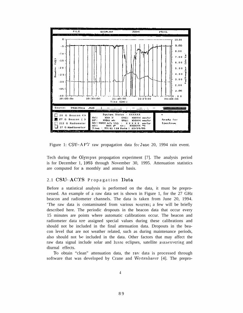
Figure 1: CSIJ–A PT raw propagation data for .June 20, 1994 rain event.

Tech during the olympus propagation experiment [7]. The analysis periodis for December 1, 1993 through November 30, 1995. Attenuation statisticsare computed for a monthly and annual basis.

2.1 CSU–ACTS Propagat i on IIata

Before a statistical analysis is performed on the data, it must be prepro-cessed. An example of a raw data set is shown in Figure 1, for the 27 GHzbeacon and radiometer channels. The data is taken from June 20, 1994.‘The raw data is contaminated from various scmrces; a few will be brieflydescribed here. The periodic dropouts in the beacon data that occur every15 minutes are points where automatic calibrations occur. The beacon andradiometer data a,re assigned special values during these calibrations andshould not be included in the final attenuation data. Dropouts in the bea-con level that are not weather related, such as during maintenance periods,also should not be included in the data. Other factors that may affect theraw data signal include solar and lunal eclipses, satellite nlaneuvering anddiurnal effects.

TO obtain “clean” attenuation data, the rav data is processed throughsoftware that was developed by Crane and Westenhaver [4]. The prepro-

4

8 9

cessilg software automatically marks data bad during calibration periods,eclipse periods and periods of ncm-therms] events (such as when the Sun isaligned along the propagation path). Diurnal effects are also automaticallyremoved by the preprocessing code. I’or effects that canl)ot be automat-ically determilied, such as maintenance periods or the occasional beacondropout, the data can be manually marked as bad. Finally, system calibra-tion is also incorporated into the prq)rocessillg code [4]. ‘1’he final outputfrom the software is calibrated attenuation data, with all bad data pointsremoved. Parameters that are used in tile statistical analysis are radiometri-cally derived attenuation (AR])) and attenuation with respect to free space(AFS)[7].

2.2 Description of Statistical Quantities

The statistical anajysis presented by Virginia ‘lkch from the olympus prop-agat ion program, was separated into two types - primary and secondarystatistics [7]. The primary statistics include cumulative distribution func-tions of the A1’S and AR.D da,ta, as well as attenuation ratio data betweentwo frequencies. A common time base is used for all the prilnary statisticscomputed so that a. valid comparison is made between the quantities of in-terest. Secondary statistics inchlde fade durations, non-fade durations andfade slope data. For these types of statistics a common time base is notused. The methods used to compute primary statistics is discussed first.

Cumulative distribution functions (CDF) are computed fo~ AILD andAI’S data at both 20 and 27 GHz. 11’he data are binned from -3.0 to 30d13 in increments of 0.1 dll. The data are presented as a percentage of timeexceeded versus attenuation level. Data used to construct the CDF plots,are taken from the 1-Hz samples of preprocessed data, w’ith no averageapplied to the data.

Attenuation ratio (R,A) data are presented here in the for]n of a per-centage of time exceecled versus dB ratio and dB level exceeded versus d]]ratio. First the data are averagecl by applyin!; a 30- second Tiloving blockaverage to remove any scintillation efl’ects. q’he attenuaticm ratio is thenobtained by dividing the 27 GHz AI’S with tlie base frequency of 20 GIIzAFS (both values are in dB). The RA values ale binned from 0.0 to 10.0 inincrements of 0.05 for all base attenuation levels greater than 1 dB. The RAdata arc also binned for different base dB levels, the base d H level rangesfrom O to 30 dIl in increments of 1 d13. RA versus dll level exceeded is usedto determine whel~ an RA value, for a specific dB level, exceeds a specific

5

9 0

value for a certain amount of time. The exceedance curves are given for 1 $.%,10%, 50%, 90% and 99% of the time.

While the primary statistics are used mainly for direct comparison ofdata between two frequencies or for scaling info] mat ion, the secondary statis-tics are used more to look at the individual chal acteristics at each frequency.They contain informaticm regarding fade duration, inter- fade duration andfade slope characteristics. Fade duration data is discussed first.

Fade duration (F])) is defined as the amount of time that the attenuationlevel (AFS) exceeds a specified threshold, q’ [7]

—. ———_—FD(AFST) = t2 – f, (1)

The bar indicates that a moving average has l)een applied to the data. inthis case a 30-second moving average is used before the fade duration com-putations were done. Similarly the non- fade or inter--fade duration (IFD)is defined as ————.

JI’D(A}’S7,) = t2 - i, (3)

where — — —.AFS < A111S7 jor’ i,<t<iz (4)

Data are presented for the number of fade eve]lts for a given threshold levelversus a specified fade duration. The percentage of time for all fades for agiven threshold level versus a specific fade duration is alsc) computed. Thethreshold level ran ges from O to 30 db in incren lents of 1 d B, while the fadeduration bins are O-1, 1-2, 2-3, 3-5, 5-6, 6-10, 10-15, 1~)-1~, 1$20, 20-30, 30-60, 60-120, 120-180, 180-300, 300-600, 600-1200, 1200-1800 and 1800-3600seconds. Non-fade duration data is colnputed in the same manner.

l{’inal]y, fade slope (II’S) information is obtained. The fade slope is com-puted after applying a 10 second moving average on the AI’S data to removesignal fluctuations due to scintillation effects. It is defined only if the attenu-ation level crosses a specified threshold and renlains either larger or smallerthan the threshold for more than 10 seconds, The fade slope for a giventhreshold crossing is defined as !7]

-—._—— ——A1’Si+5 – AFSi_5

‘Si = ‘- - - - - - 10

6

91

(5)

where AI’S is given as

(6)

and i is the index value when the attenuation crosses a specified threshold.The threshold values range from O to 30 dll in increments of 1 dB, while thefade slope values are binned from -1.25 to 1.25 d13/sec in increments of 0.05dI1/scc.

Primary and secondary statistics am computed on a monthly basis andannually for the period of I)ecember 1, 1993 to November 30, 1995. Resultsobtained at CSU for the two year period are given in Appendix A.

3

3.1

CSU–CHILL F’olarimetric Radar Data

Radar Description

The CIIII,I., radar has an historic past as it was one of the first radars to uti-lize polarization cliversity. ‘J’he radar \vas originally design a]ld constructedjointly by the University of Chicago and the Illi~lois Water Survey under theguidance of Mueller and Atlas [2]. In 1990, tile CHILI, radar was movedto its present location outside of Greeley, Colorado and is now used exclu-sively as a research radar operated by CSIJ u]lder the sponsorship of theNational Science l’ounda,tion. It is a fully polarimctric S- band radar thatcan alternately send two orthogonally polarized signals and simultaneouslyreceive the co- and cross- polarized signals. With recent upgrades made tothe radar it is now ranks as one of the top radars of its kind. A summaryof the system characteristics are given ill q’able 1

3 . 2 R a d a r O b s e r v a b l e

The CSIJ-CHIl,L radar transmits and receives both horizontal and verticalpolarizations. Being able to measure both the copolar and cross--polar re-turns a~lows measurements of such quantities as the horizollt al reflectivity(Z}l ), differential reflectivity (ZI)R), the specific differential phase betweenthe 11 and V copo]ar signals (l{DP) and the differential propagation phaseshift (+DP). ~’he correlation coefficient between the two copola.r signals(pHv) and the linear depolarization ratio (LDR) are alsc, measured. I’heradar obscrvables can be defined in terms of tile forward and back scatter-ing amplitudes and the raindrop size distribution. ‘I’he first subscript of the

92

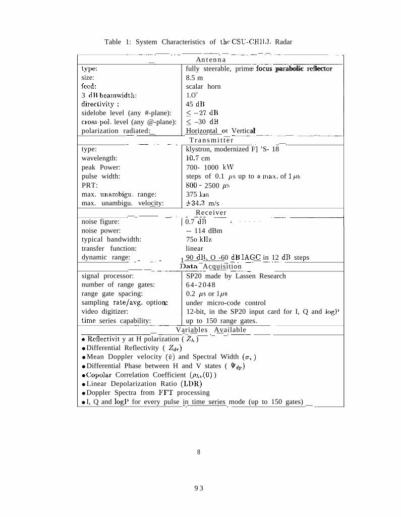
Table 1: System Characteristics of the CSU-CHILL Radar

————. .—— . . .. ——— —-—. — —— .—— — .—. ——Antenna—.

type:

:1

fully steerable, prime focus parabolic reflectorsize: 8.5 mfeed: scalar horn3 dll beamwidth: 1.OO

directivity : 45 d~sidelobe level (any #-plane): s –27 dBcross-pol. level (any @-plane): ~ –30 dBpolarization radiated: Horizontal or Vertical.—— —. .—— —- —— __ _

.—— ——— — ——. —type:wavelength:peak Power:pulse width:PRT:max. unambigu. range:max. unambigu. velocity:—.

.—.. ——— .——..

T r a n s m i t t e r ————. ..— ..—.klystron, modernized F] ’S- 1810.7 cm700- 1000 kWsteps of 0.1 ifs up to a nlax. of 1 KS800- 2500 ps375 km+34.3 m/s

Receiver——— —— —-_noise figure: I 0.7 dEi ‘ - - - - - ‘“---–~noise power:

- - 1

-- 114 dBmtypical bandwidth: 75o klIztransfer function: lineardynamic range: 90 d]], O -60 dB IAGC in 12 dIl steps—— —.— ——_———_ _.— .—. .——

l>ata Acquisition.—— —.. .—

--= 1

——-— —-— —signal processor: SP20 made by Lassen Researchnumber of range gates: 64 -2048range gate spacing: 0.2 ps or lpssampling rate/avg. option: under micro-code controlvideo digitizer: 12-bit, in the SP20 input card for I, Q and logPtilme series capability: up to 150 range gates.—.—

Variables Available—— — .— -.. —___ ._ —_. _; R,eflectivit y at H polarization ( Z~ )● Differential Reflectivity ( Z~T)● Mean Doppler velocity (o) and Spectral Width (o,, )● Differential Phase between H and V states ( IPdP)● Copolar Correlation Coefficient (p~l,(0) )● Linear Depolarization Ratio (LDR)● Doppler Spectra from I?FT processing● I, Q and logP for every pulse in time series mode (up to 150 gates)-.————-—. — .

8

9 3

polarization states given in the following equations refers to the receivedpolarization state, while the second subscript refers to the transmitted po-larization state. The horizontal and vertical reflectivity are defined by

A4ZHH,VV = -—-—

JoHH,vv(D)N(lj)dD, m7\i6rn- 3 (7)

7;51}(12

where OHH,VV (D) are the copolar radar cross sections at the horizontal andvertical polarizations, II([ = (C7 - 1 ) / (CT + 2), E, is the dielectric constantof water and A is the wavelength [5]. Differential reflectivity is defined as

r

ZDR = 10 log -$;;-, dl? (8)

Defining JHH and JVV as the forward scatteri]lg amplitudes of the H and Vpolarized waves, the specific differential phase is given as

Then ~DP is defined as

J

r 241)F’ = 21{DP(r)dr (deg) (lo)TI

where ~D1> is the two--way differential phase between range lc,cations, r] andr2. If the backscatter amplitudes for the horizoIltal and vertical polarizationsare defined as SHH and Svv, then the cross–correlation coefficient is given

The linear depolarization ratio can also be defined in terms of the backscatteramplitudes

(12)

The variable N(D) is the raindrop size distribution in equations 7-12 and isthe number of raindrops per unit volulne per unit size inter~al D to D + 6D,where D refers to the equivalent spherical dia]neter [6].

Each polarimetric parameter provides information about the type ofparticles present in a given radar range resolution volume. For instance,information regarding a particle’s shape can be obtained from the differ-ential reflectivity, while information about a particle’s orientation can be

9

94

obtained from the linear dcpolarizatioli ratio. Specific difl’ercntizd phase issensitive only tcj non-spherical particles such as oblate rain d] ops or alignedic.c crystals. While each of these parameters J)rovide inforn]atioll on theirown, looking at a combil~ation of polar imetric lmramel,ers caJl give an evengreater insight to what is occurring; in a particular storln cell. For example,reflectivity and differential reflectivity used together can be a good indicatorto determine if a range resolution volu]ne contains hail particles. ‘1’ypically,if hail is present the’ rwflcctivity values tend to be high, while the tumblingnature of hail stones results in low values for ditTerential reflectivity. This isjust one of many examples of how polarimctric parameters can be used indescribing the internal structure of storm events.

3.3 Attenuation Estimates

To obtain K–band attenuation estimates from S-band reflectivity data, sim-ulations were obtained by ‘varying the parameters of a given drop size dis-tribution (11 S1>). IJsing a Mie scdution for spherical water particles, propa-gation variables such as K- band attenuation and S- band reflectivity werecomputed using a wide range of DSD parameters. III this case a. gamma1)S1) was used

N(D) == A’(,nwLe-~]) (13)

where3.67 + m

7 = -–-6;-””(14)

and N(D), given in mm--’ 3,3, is the number of drops per unit volume perunit size interval, D is the equivalent drop size diameter in mm, A’. is giveni n m m- l - mm - 3 , Do is the median drop size in mm and 7n is the shapefactor. l’hc I)SD triplets (No, Do, 772) are varied as follows: 100 < No ~50000, 1 < DO s 4 and O < m < 5. Results of the simulation are shown inFigure 2. Each pc)int on the scatter plot represents K-band attenuation andS- band reflectivity for a given DSD triplet. The entire range of triplets arerepresentative of actual drop size distributions for a \vidc vm-iety of rainfallevents [1].

The S- band reflectivity/K-band attenuation curves are obtained by ap-plying a power function fit to the simulated data. The equation that relatesS-band reflectivity to K--band attenuation is given by

AK =:: a (lOZs/lO)~

10

95

(15)

Scatter Plot of Ka-Band Attenuation versus S-Band Reflectivity- -25

20

15

10

5

‘-— ‘T--—~--—T–— 1 _ — . . .

20 GHz Attenuation Curve —T

1’?,-. . . .: >L!. ,..

Lo -—-—~-– _—_J___ 4... ~

- 2 0 25 30 35 50 55 60S-Band Re~jctivi~4~BZ)

Scatter Plot of Ka-Band Attenuation versus S-Band Reflectivity- -

Figure 2:

15

0

5

–—— “ — - r - — - — — - ~ — - - -

27 GHz Attenuation Curve — T

o20 25 30 35 40 50 55 60

S43and F{eflectivity4~BZ)

Attenuation for 20 and 27 GHz versus reflectivity at 3 GHz,obtained using a Mie solution for spherical particles.

11

9 6

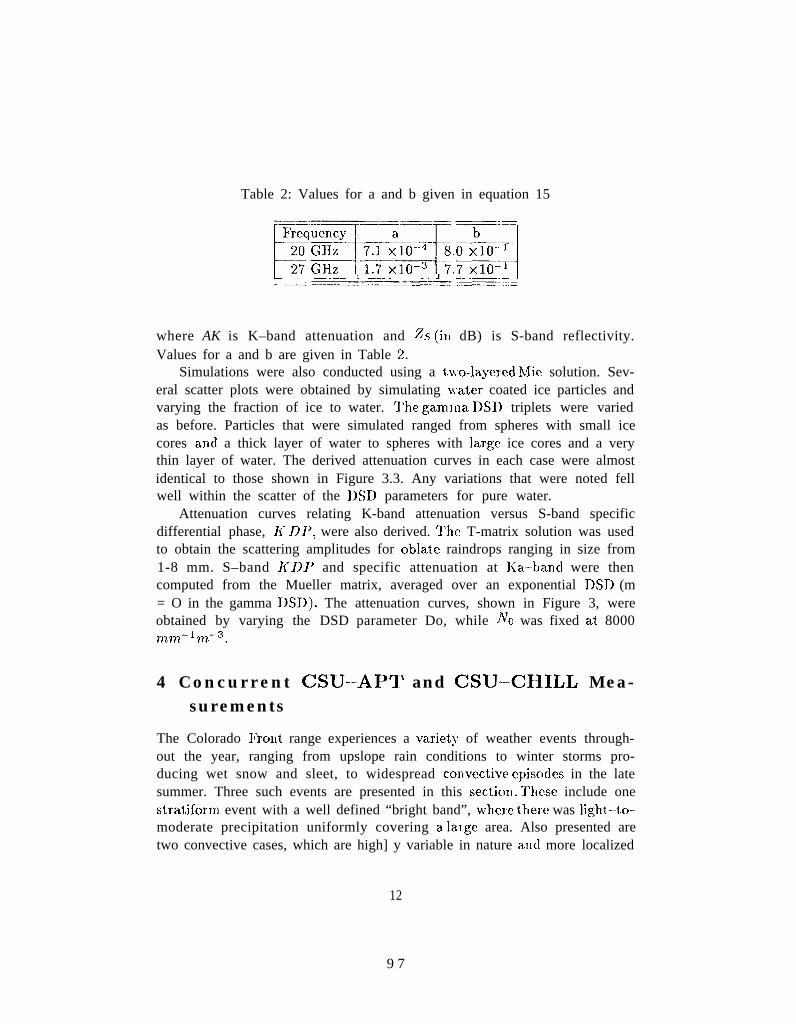
Table 2: Values for a and b given in equation 15

~— .~—.—–_—.-L—-J——— —————= :.——_—. -=

where AK is K–band attenuation and ZS (ill dB) is S-band reflectivity.Values for a and b are given in Table 2.

Simulations were also conducted using a tw’o-]aye]ed Mie solution. Sev-eral scatter plots were obtained by simulating w’ater coated ice particles andvarying the fraction of ice to water. q’he gamlna DSD triplets were variedas before. Particles that were simulated ranged from spheres with small icecores and a thick layer of water to spheres with large ice cores and a verythin layer of water. The derived attenuation curves in each case were almostidentical to those shown in Figure 3.3. Any variations that were noted fellwell within the scatter of the I)SD parameters for pure water.

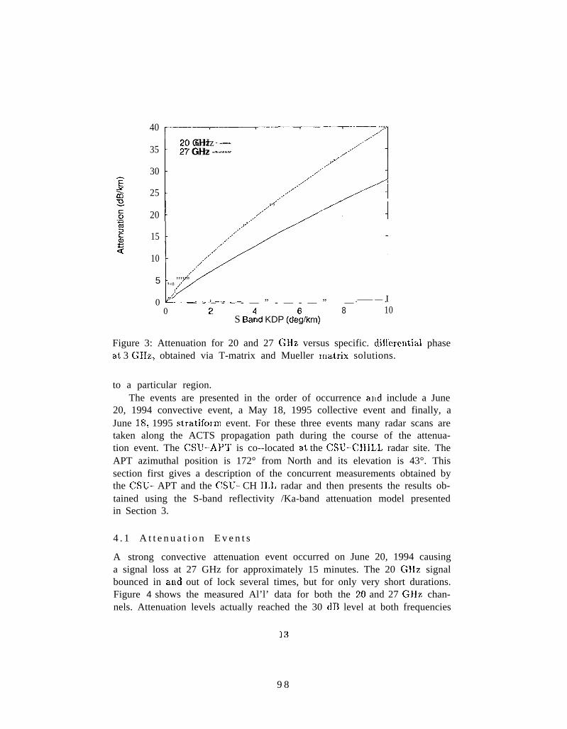
Attenuation curves relating K-band attenuation versus S-band specificdifferential phase, I{ D-F’, were also derived. The T-matrix solution was usedto obtain the scattering amplitudes for oblate raindrops ranging in size from1-8 mm. S–band 1{.D.P and specific attenuation at Ka–band were thencomputed from the Mueller matrix, averaged over an exponential DSD (m= O in the gamma DSD). The attenuation curves, shown in Figure 3, wereobtained by varying the DSD parameter Do, while IV. was fixed at 8000mm-lm–3.

4 Concurrent CSU--AP’J’ and CSU-CHILL Mea-surements

The Colorado l’r-ont range experiences a variet~ of weather events through-out the year, ranging from upslope rain conditions to winter storms pro-ducing wet snow and sleet, to widespread colivective episc)des in the latesummer. Three such events are presented in this secticm. These include onestratiform event with a well defined “bright band”, whele there was light–to-

moderate precipitation uniformly covering a lalge area. Also presented aretwo convective cases, which are high] y variable in nature a]ld more localized

12

9 7

40

1~

——7 .—-———-—7-— —.—— ..,...”

2C~ GHz -–-.--’,,,

35,.-

27 GHz ------ ,,-,.-.> ’-,.-

30,.-’,,,’,.-,,-,.,

25 ..”,.,/,”’,.,

20,.”,,,

/,”,.-,,,15 ,,,,,,

,,. ”,/,10

v

,,.’,/.”

5 ,<8 ’’’’’”,,,

0 ““ — - – - – - — ” - — - — ” — I.—— — .0 2 8 10

S Ba~d KDP (de~/km)

Figure 3: Attenuation for 20 and 27 GHz versus specific. dif~erential phaseat 3 GHz, obtained via T-matrix and Mueller ]natrix solutions.

to a particular region.The events are presented in the order of occurrence and include a June

20, 1994 convective event, a May 18, 1995 collective event and finally, aJune 18, 1995 stratiform event. For these three events many radar scans aretaken along the ACTS propagation path during the course of the attenua-tion event. The CSU-APT is co--located at the CSU-CHILL radar site. TheAPT azimuthal position is 172° from North and its elevation is 43°. Thissection first gives a description of the concurrent measurements obtained bythe CSIJ- APT and the CSU- CH 11.1, radar and then presents the results ob-tained using the S-band reflectivity /Ka-band attenuation model presentedin Section 3.

4 . 1 A t t e n u a t i o n E v e n t s

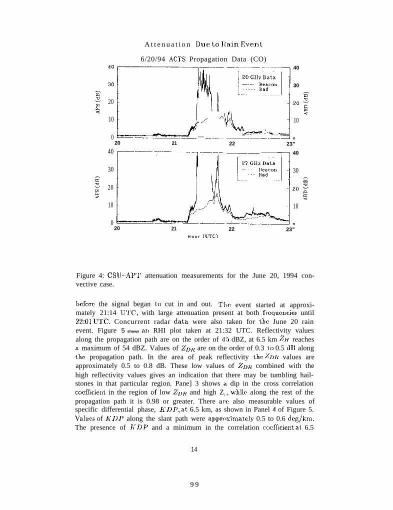
A strong convective attenuation event occurred on June 20, 1994 causinga signal loss at 27 GHz for approximately 15 minutes. The 20 CXHZ signalbounced in and out of lock several times, but for only very short durations.Figure 4 shows the measured Al’l’ data for both the 20 and 27 GHz chan-nels. Attenuation levels actually reached the 30 dB level at both frequencies

13

98

A t t e n u a t i o n l)ue t.o Rain Everlt

6/20/94 ACTS Propagation Data (CO)

20

10[~

~.Y

,. /,

0 -.— -..—.——.. . ..—— — L—-— -=._L. ._

. ..!JL j-......e....& . . .

40

30

20

10

0

40

30

10

n20 21 22 23”-.—–-—–— —-———_ n ——-— __ —— 40

30

10

n20 21 22 23”

H o u r fUTC)

Figure 4: CSU--AI’T attenuation measurements for the June 20, 1994 con-vective case.

before the signal began to cut in and out. ‘1’lle event started at approxi-mately 21:14 UT(I, with large attenuation present at both fwquencies until22:01 U’TC. Concurrent radar data were also taken for the June 20 rainevent. Figure 5 shows all RHI plot taken at 21:32 UTC. Reflectivity valuesalong the propagation path are on the order of 45 dBZ, at 6.5 km ZH reachesa maximum of 54 dBZ. Values of ZDR are on the order of 0.3 to 0.5 dB alongthe propagation path. In the area of peak reflectivity the XI)}{ values areapproximately 0.5 to 0.8 dB. These low values of ZDIl combined with thehigh reflectivity values gives an indication that there may be tumbling hail-stones in that particular region. Pane] 3 shows a dip in the cross correlationcoefficient in the region c)f low Z1)~ and high Z}:, while along the rest of thepropagation path it is 0.98 or greater. There are also measurable values ofspecific differential phase, l{DF’, at 6.5 km, as shown in Panel 4 of Figure 5.VaJues of l{D.P along the slant path were appr{,ximately 0.5 to 0.6 deg/km.The presence of A’-DP and a minimum in the correlation ccwficient at 6.5

14

99

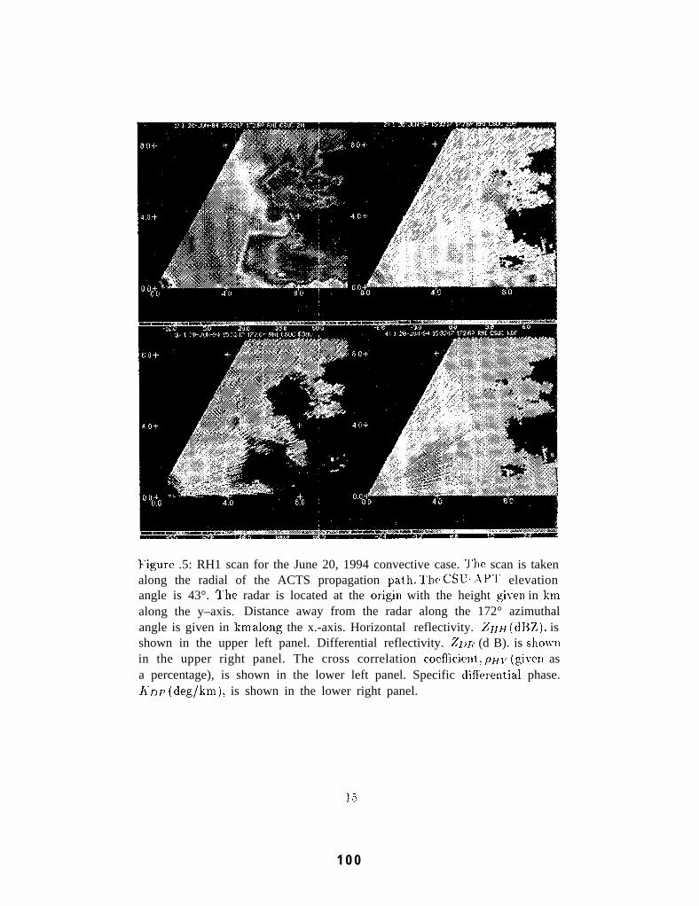
k’i.gure .5: RH1 scan for the June 20, 1994 convective case. The scan is takenalong the radial of the ACTS propagation path. The CSU .~I’T elevationangle is 43°. The radar is located at the origin with the height given in kmalong the y–axis. Distance away from the radar along the 172° azimuthalangle is given in km dOllfj the x.-axis. Horizontal reflectivity. ZHH (dHZ). isshown in the upper left panel. Differential reflectivity. ZIj~ (d B). is sho~rnin the upper right panel. The cross correlation coeflicie]lt, p}lv (given asa percentage), is shown in the lower left panel. Specific difl’erential phase.I{DP (deg/km), is shown in the lower right panel.

~ ,j

1 0 0

ACTS Data - Convective Case5/1 8/95 ACTS Propagation Data (CO)

1 2 0 — - — T - — — - — - — — — — — — —“

-L

100 EZEZI 4), f~“”1. ;: ;;

g 8.0 /3

j:c

“; 6 . 0. 1

3c /j’ L

g 4.0 i

<)

d?

i.8.>

;% *. /5

2 0 . . . ” .$

nn .—A.—— —.

120

100

8.0

60

40

20

00“,”

200 20.1 20.2 20.3 20,4 20.5 20.6 20,7 20.8 209 21.0-’ -

1 5 . 0 ~-—-v———- — - — —“–— 1

->0,0 20.1 20.2 20.3 20.4 20.5 20.6 20.7 20.6 20.9 21.0

Hour (U1-C)

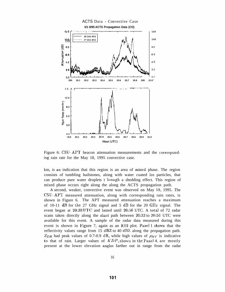
Figure 6: CSU-APT beacon attenuation measurements and the correspondi-ng rain rate for the May 18, 1995 convective case.

km, is an indication that this region is an area of mixed phase. The regionconsists of tumbling hailstones, along with water coated ice particles, thatcan produce pure water droplets t hrou,gh a shedding effect. This region ofmixed phase occurs right along the along the ACTS propagation path.

A second, weaker, convective event was observed on May 18, 1995. TheCSU-APT measured attenuation, along with corresponding rain rates, isshown in Figure 6. The APT measured attenuation reaches a maximumof 10-11 dB for the 27 GHz signal and 5 dB for the 20 Gllz signal. Theevent began at 20:30 U2’C and lasted until 20:.56 UTC. A total of 72 radarscans taken directly along the slant path between 20:32 to 20:56 UTC wereavailable for this event. A sample of the radar data measured during thisevent is shown in I?igurc 7, again as an R.HI plot. Pane] 1 shc)ws that thereflectivity values range from 15 dBZ to 40 d13Z along the propagation path.ZDFt had peak values of 0.7-0.9 dll, while high values of pl{}z is indicativeto that of rain. Larger values of A’DF’, show]l in the Panel 4, are mostlypresent at the lower elevation ZLllgk farther out in range from the radar

16

101

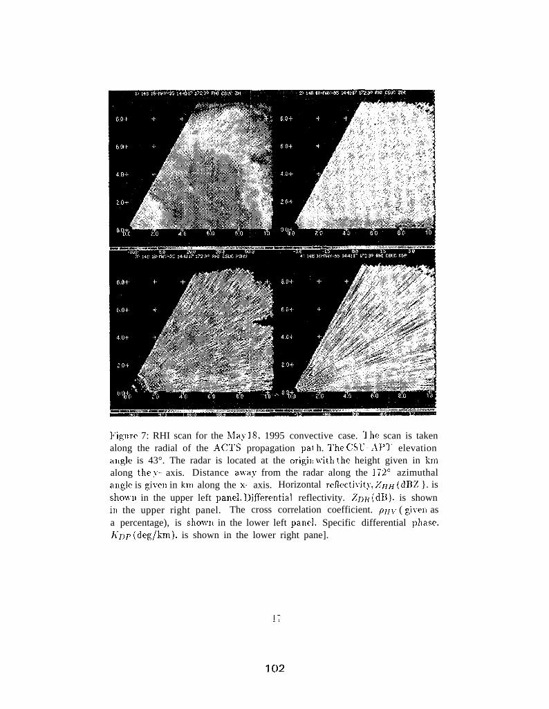
Figure 7: RHI scan for the May 18, 1995 convective case. The scan is takenalong the radial of the .4CTS propagation pa{ h. The CSL- AP2’ elevationang]e is 43°. The radar is located at the origin w’ith the height given in kmalong the y- axis. Distance a~vay from the radar along the 172° azimuthalangle is given in km along the x- axis. Horizontal reflectivit~’. ZHH (dIIZ }. isshowm in the upper left panel. IIiflerential reflectivity. 2])}{ (d}\). is shownil] the upper right panel. The cross correlation coefficient. p~l~ ( given asa percentage), is shomw in the lower left pane]. Specific differential phase.l(DP (deg/lml), is shown in the lower right pane].

ACTS Data - Stratiform Case6/1 8/95 ACTS Propagation Data (CO)

Su &oc

“: 6 . 0Dci? 4 . 0<

2.0

..-3.0 3.2 34 3.6 3.8 4.0 4.2 4.4 4.6 4.8 5.0

10.0 ➤ -—.r-–--r-------- -. 19.0

8.0

.$ 3 0

K 2.0

1.0

0.0

1?0

1 0 0

8 0

6 0

4 0

2 0

0 0

3.0 3.2 34 3.6 3.8 4.0 4.2 4.4 4.6 46 50

H o u r (UTC)

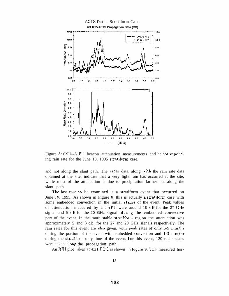
Figure 8: CSU--A I’T beacon attenuation measurements anding rain rate for the June 18, 1995 stratiform case.

he correspond-

and not along the slant path. The radar- data, along with the rain rate dataobtained at the site, indicate that a. very light rain has occurred at the site,while most of the attenuation is due to precipitation farther out along theslant path.

The last case to be examined is a stratiform event that occurred onJune 18, 1995. As shown in Figure 8, this is actually a stratiform case withsome embedded convection in the initial stages of the event. Peak valuesof attenuation measured by the APT were around 10 d]] for the 27 GHzsignal and 5 d13 for the 20 GHz signal, duri]~g the embedded convectivepart of the event. In the more stable stratiforlo region the attenuation wasapproximately 5 and 3 dB, for the 27 and 20 GHz signals respectively. Therain rates for this event are alsc) given, with peak rates of only 6-9 mm/hrduring the portion of the event with embedded convection and 1-3 mm/hrduring the stratiform only time of the event. For this event, 120 radar scanswere taken along

An RH1 plotthe propagation path.aken at 4:21 U’ll C is shown

18

n Figure 9. ‘l’he measured hor-

1 0 3

izontal reflectivity was about 45 d13Z in the region of the bright band, whilevalues of 30 dHZ are seen along the propagation path below the reflectivitybright band. The height of the reflectivity bright band is approximately2,45 km. ZDR values in the melting layer were approximately 1.0- 1.5 dll,with values of 0,5--0.8 dB below the melting layer. The p}ll, data exhibitsthe typical decrease in Inagnitude in the melting region, with values drop-ping to 0.93. The final radar parameter given in this RH1 plot is the lineardepolarization ratio (LI)R) and it has values up to -18 dB in the meltinglayer.

‘1’hc next step in the analysis process is to use the radar information asinput to the propagation model on a case-by-case basis. Results using theS--band reflectivity/Ka-band attenuation model are presented in the nextsection for the three case studies.

4 . 2 A t t e n u a t i o n E s t i m a t e s

Attenuation estimates have been computed using the S band reflectivity /Ka-band attenuation model derived in Section 3.3, Only the reflectivity valueshave been used to model the cases described i], the previous section (A”DPestimates were used in the June 20, 1994 convective case), while the polari-metric parameters ZDR, l{DF’ and pHI/ were used to determine the lengthof the attenuation path. These polarimetric parameters are dependent onthe elevation angle of the radar, therefore a correction factor is used to ob-tain values of ZD}l and A’DP for an elevation angle of OO. q’he correctedvalues are used as input to the attenuation model.

Radar scans were taken directly along the ACTS propagation path witha range resolution of 150 m. Reflectivity data at 3 GHz wele taken atthe 150 m increments and used to determine the corresponding 20 and 27GHz attenuation estimates from the attenuation curves given in Figure 2.‘l’he Ka-band attenuation estimates were then lnultiplied by the appropriatedistance along the propagation path.

For the June 20, 1994 convective case, 43 raclar scans were taken through-out the duration of the event. Ka-band attenuation estimates were derivedfrom S-band reflectivity data using the procedure described above. For thisparticular event S-band I{DP data are alsc) used to derive Ka-band atten-uation estimates. The results are shown in Figure 10

As seen in Figure 10, the CSU–CHIL1, reflectivity based attenuationestimates follow the attenuation measurements obtained from the APT veryclosely. The maximum difference is about 5 db, while for the most part the

19

1 0 4

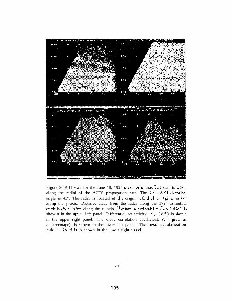
Figure 9: RHI scan for the June 18, 1995 stratiform case. The scan is takenalong the radial of the ACTS propagation path. The CSL7- .\Pl”’ elevationangle is 43°. The radar is located at tile origin ~vith the heisht given in kmalong the y–axis. Distance away from the radar along the 172° azimuthalangle is given in km along the x--axis. }] OrbOntd IWflWtiVit~. ~HH (d13Z). isshow-n in the upper left panel. Differential reflectivity. Z~)~ ( dB ). is shov-nin the upper right panel. The cross correlation coefficient. pHlf (given asa percentage). is shown in the lower left panel. The linear depolarizationratio. I,DI{ (dII). is showm in the lower right l~anel.

2(I

1 0 5

40 r—-—z7—-zT—-~-T 7-—1 -—–-

() l-—-.–.:— 1 .—__ 1 ___._L — — — – d . _ _ _ _ _

2 1 . 5 21.55 2 1 . 6 2 1 . 6 5 21.7 21.75 21.8 21.85 21.9Hour (UTC)

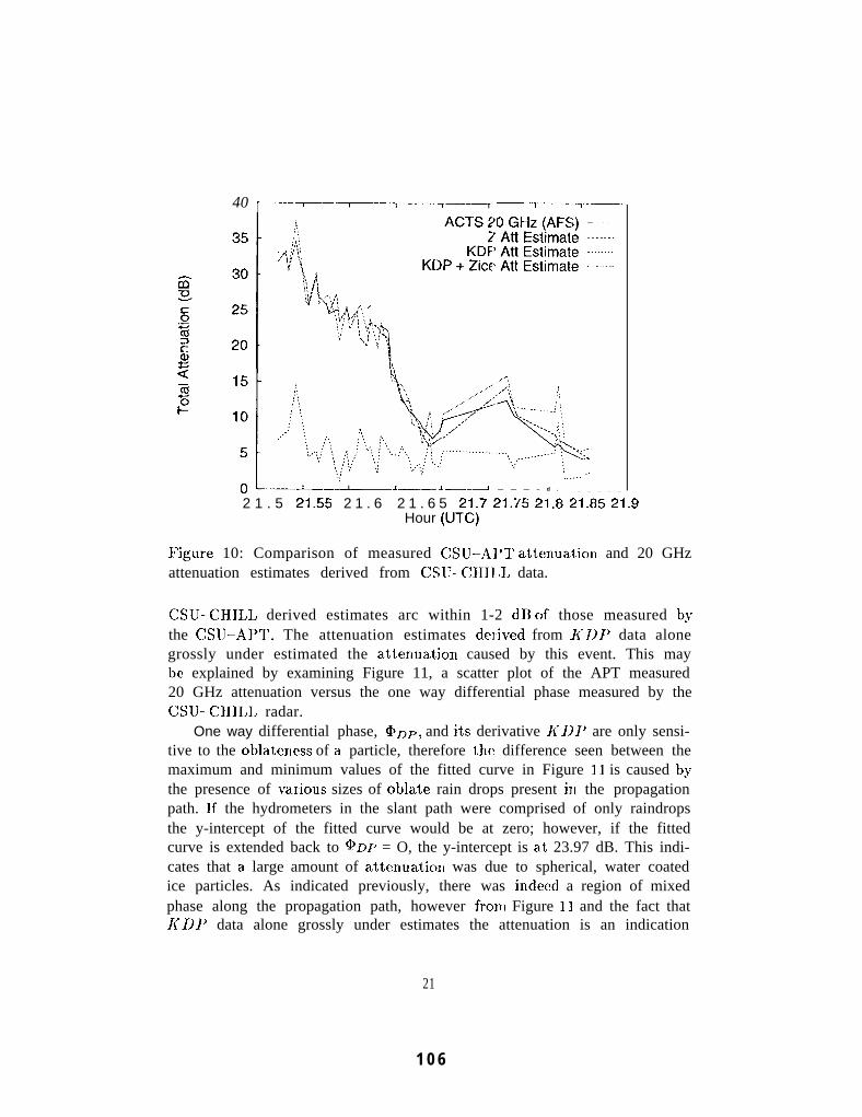
Figure 10: Comparison of measured CSU--AI’T attenuatic,n and 20 GHzattenuation estimates derived from CSIJ--CHII ,1, data.

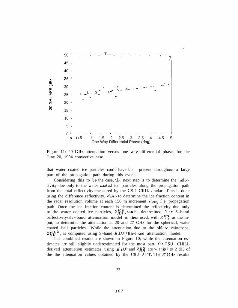
CSU-CHILL derived estimates arc within 1-2 dB c)f those measured bythe CSU–AP1’. The attenuation estimates delived from 1{1)1’ data alonegrossly under estimated the atteriuation caused by this event. This maybc explained by examining Figure 11, a scatter plot of the APT measured20 GHz attenuation versus the one way differential phase measured by theCSU- CIIII,I, radar.

One way differential phase, @DP, and its derivative h’])]’ are only sensi-tive to the oblateness of a particle, therefore the difference seen between themaximum and minimum values of the fitted curve in Figure 11 is caused bythe presence of va,rious sizes of obla.te rain drops present in the propagationpath. If the hydrometers in the slant path were comprised of only raindropsthe y-intercept of the fitted curve would be at zero; however, if the fittedcurve is extended back to @Dp = O, the y-intercept is at 23.97 dB. This indi-cates that a. large amount of attenuaticJ1l was due to spherical, water coatedice particles. As indicated previously, there was indeed a region of mixedphase along the propagation path, however fron) Figure 11 and the fact thatA’D1’ data alone grossly under estimates the attenuation is an indication

21

1 0 6

.

50 ~--,_—r .—_-..T–—_.. ~_‘ - ~–~-—- T ‘-.

745 -

40 -

35 ‘

30 -

25 -

20 -

15 -

10 -

5 -

100

00 .—-- --- —-

o_——————w * _y_”_-—-- 0

~J&/ .0 ~0 0

0

0 (-—-L_J-__L___..L___ l__L _L–..—L —.--i

o ().5 ! 1.5 2 2.5 3 3.5 4 4.5 5One Way Differential Phase (deg)

Figure 11: 20 GHz attenuation versus one way differential phase, for theJune 20, 1994 convective case.

that water coated ice particles could have bee], present throughout a largepart of the propagation path during this event.

Considering this to be the case, the next step is to determine the reflec-tivity due only to the water coated ice particles along the propagation pathfrom the total reflectivity measured by the CSU-CHILI. radar. ‘l’his is doneusing the difference reflectivity, ZDp, to determine the ice fraction content inthe radar resolution volume at each 150 m increment along tile propagationpath. Once the ice fraction content is determined the reflectivity due onlyto the water coated ice particles, Z~~~, can be determined. The S–bandreflectivity/Ka--band attenuation model is then used, with Z{{!? as the in-put, to determine the attenuation at 20 and 27 GHz for the spherical, watercoated hail particles. While the attenuation due to the ob]ate raindrops,

~IIIJ‘AIN, is computed using S–band A’DP/Ka-l)and attenuation model.The combined results are shown in Figure 10; while the attenuation es-

timates are still slightly underestimated for the most part, the CSU- CHILLderived attenuation estimates using KDP and Z~~~ are wit]lin 1 to 2 dJ3 ofthe the attenuation values obtained by the CSIJ--APT. The 27 GHz results

22

1 0 7

5 0 —--r-y

[“

— -——-T-—–—- 7—-Y —-———— -T’ --—: :?., :;~

45ACTS 27 Gttz (AFS) ----; ; ,,’. , ,.,; :. ,: ; ,< , Z Att Estimate ----

‘., ti’j:.’’:d, > KDP ~ Zice Att Estimate ~~~~~~~~40 ., :: .’! : . . .., ~ \,,,. ,, ,, ,.,

:,. , :, !J,., ,, ,, :,,,35

,!,, :,,:,, .,, ;

5t

() l.—___L_._.L.1____ L—..J. —.—- L..—.

21.5 21.55 21.6 21.65 21.7 21.75 21.8 21.85 21.9Hour (UTC)

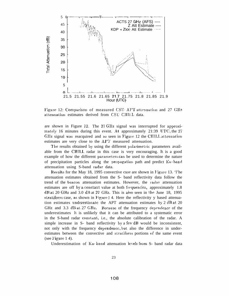
k’igure 12: Compariscm of measured CSU- A1’T attcnuatio]l and 27 GHzattcnua,tion estimates derived from CSIJ- CHIII, data.

are shown in Figure 12. The 27 GHz signal was interrupted for approxi-mately 16 minutes during this event. .LIt approximately 21:39 UT’C, the 27GJIz signal was reacquired and ZLS seen in ?i’igu]e 12 the CHI1,I, attcmuatiollestimates are very close to the AP’3’ measured attenuation.

l’he results obtained by using the different polarirnetric parameters avail-able from the CHII,L radar in this case is very encouraging. It is a goodexample of how the different PMZLInet12rS can be used to determine the natureof precipitation particles along the propagatiol( path and predict Ka-ba.ndattenuation using S-band radar data.

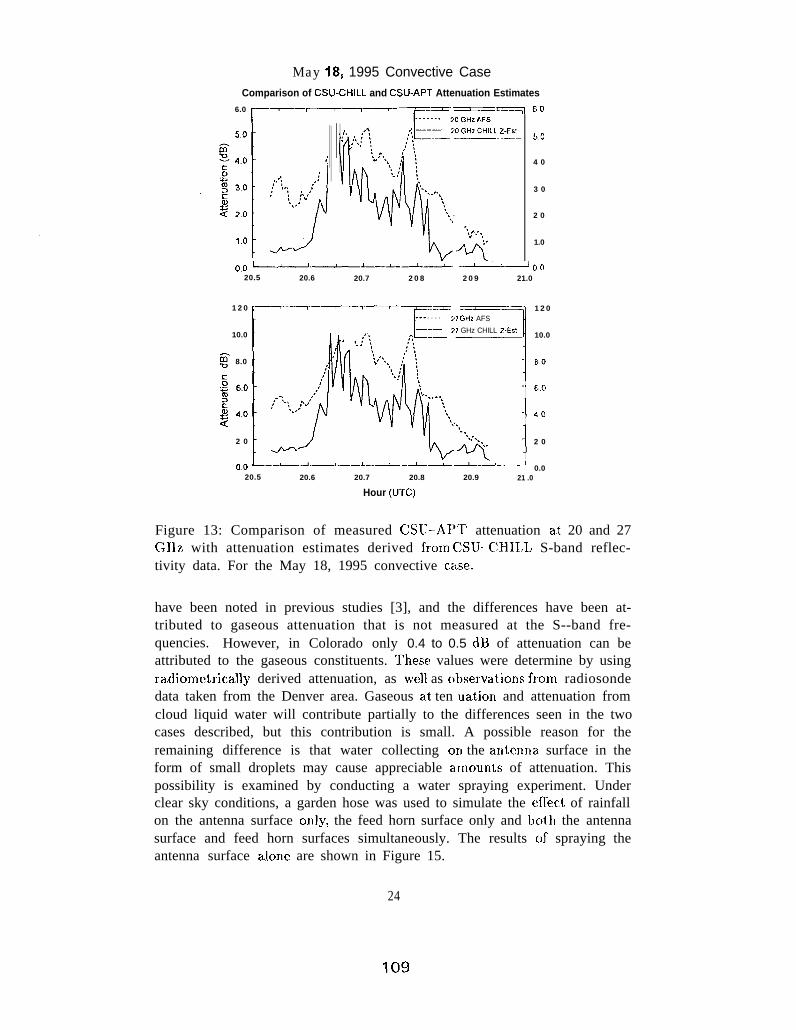
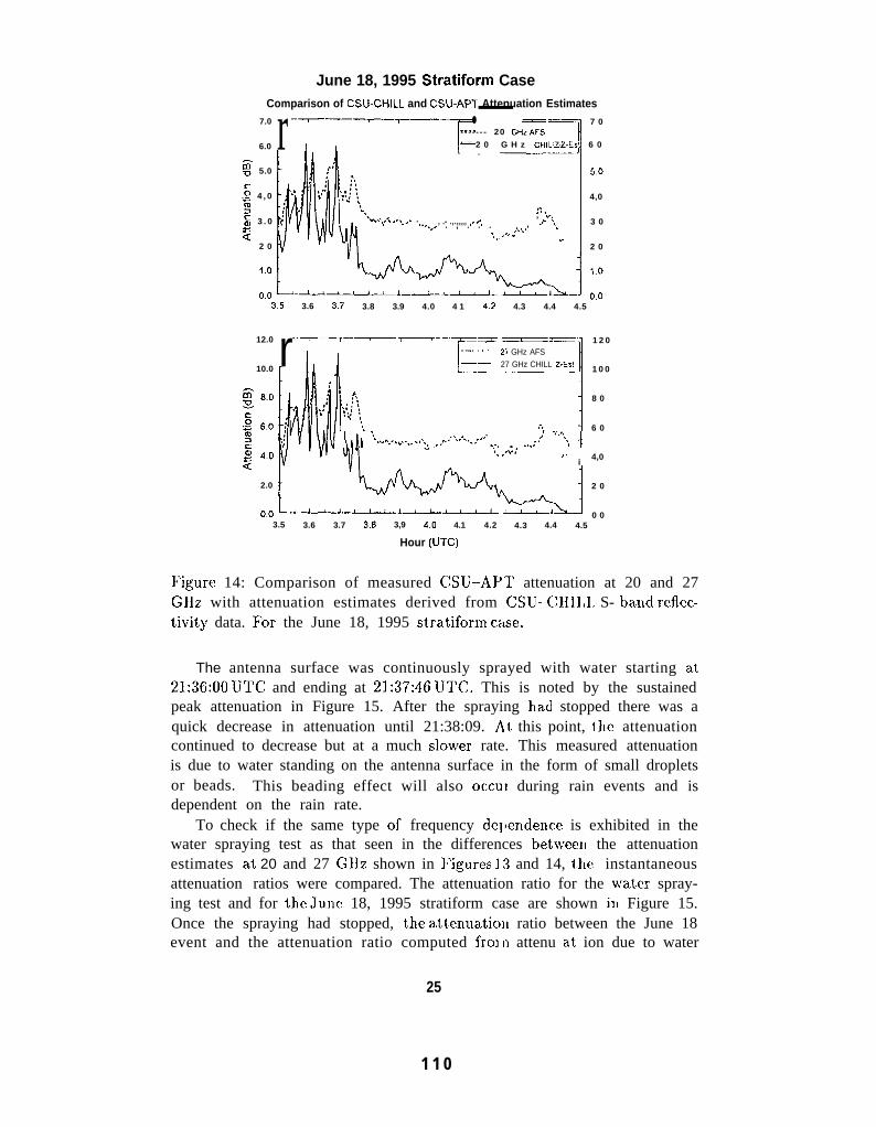
l{esults for the May 18, 1995 convective case are shown in ]’igure 13. ‘l’heattenuation estimates obtained from the S- band reflectivity data follow thetrend of the beacon attenuation estimates. However, the yadar attenuationestimates are off by a col[stant value at both fr[’quencies, approximately 1.8d]] at 20 GHz and 3.0 d]] at 27 GHz. This is also seen in the June 18, 1995stratiform case, as shown in l’igure J 4. Here the reflectivity y based attenua-tion estimates underestilnate the APT attenuation estimates by 2 dIl at 20GHz and 3.3 dB at 27 GHz. Hecause of the frequency depcmdence of theunderestimates it is unlikely that it can be attributed to a systematic errorin the S-band radar cc)nstant, i.e., the absolute calibration of the radar. Asimple increase in S- band reflectivity by a few dB would be inconsistent,not only with the frequency depcndencc, but also the difference in under-estimates between the convective and stratifor~ll portions c)f the same event(see l’igure 1 4).

Underestimation of Ka-band attenuation levels froln S- band radar data

23

108

—

May ’18, 1995 Convective CaseComparison of CSU-CHILL and CSU-APT Attenuation Estimates

6.0 r_——-,~--- ~s —I====J 60

.Z?: 50

4 0

3 0

2 0

1.0

0,0 L-—AJ.—L_——L_— —L_-._l 00

20.5 20.6 20.7 2 0 8 2 0 9 21.0

1 2 0

10.0

g 8.0

2 0

nn

r—Y—,-z-l—-T-

Tz=: — —

. . . . . . . >7 GHz AFS—-— 727 GHz CHILL Z-ESt

L__—_l.—~_l.—-- .-L--— —— I---20.5 20.6 20.7 20.8 20.9 21

1 2 0

10.0

8.0

&o

40

2 0

0.0.0

Hour (UTC)

Figure 13: Comparison of measured CSU--AP”T attenuation at 20 and 27GHz with attenuation estimates derived frcjm CSU-CHII,L S-band reflec-tivity data. For the May 18, 1995 convective case.

have been noted in previous studies [3], and the differences have been at-tributed to gaseous attenuation that is not measured at the S--band fre-quencies. However, in Colorado only 0.4 to 0.5 dB of attenuation can beattributed to the gaseous constituents. ‘1’hese values were determine by usingradiometrically derived attenuation, as well as c)bservations flom radiosondedata taken from the Denver area. Gaseous at ten uation and attenuation fromcloud liquid water will contribute partially to the differences seen in the twocases described, but this contribution is small. A possible reason for theremaining difference is that water collecting on the antenna surface in theform of small droplets may cause appreciable alnounts of attenuation. Thispossibility is examined by conducting a water spraying experiment. Underclear sky conditions, a garden hose was used to simulate the effect of rainfallon the antenna surface o]lly, the feed horn surface only and bc)th the antennasurface and feed horn surfaces simultaneously. The results of spraying theantenna surface alone are shown in Figure 15.

24

109

June 18, 1995 Stratiform CaseComparison of CSU-CHILL and CSLJ-APT Attenuation Estimates

7.0 r———r—r—- T.— —7 7 0- - - - - - - 20 GHZAFS

6.0 11 ‘ - — 2 0 G H z CHILL Z-ES! 6 0L _ _—)

= 5.0 50

.s 4 , 0 4,0z3 ,$

; 3 . 0,.*‘.%. ,,, ,-, , ,-,

> /,. . , .- .,.,,,,, ,, ,., , .? ‘~, 3 0%.-. . , . . .

z,,, “,+

‘%2 0

,.2 0

—..—.-4_A&vka&-~ O.

v.

0.0 ~~3,5 3.6 37 3.8 3.9 4.0 4 1 4,2 4.3 4.4 4.5

12.0

10.0

2.0

r——Y-T—— T——---7-- —.r:Z —=-

1~-. . . . . . 27 GHz AFS

I—. 27 GHz CHILL Z-ES!-. ——1

;,. I\Nu Lb “$.”-$-..’$...--”’’’’’’”’”.-. . ...’” ““’’”$ +i. ,.%.,’ ,.

i

0.0 ~~—L—L-- L—_I_— ~Lk-.J3.5 3.6 3.7 3,8 3,9 4.0 4.1 4.2 4.3 4.4 4.5

1 2 0

1 0 0

8 0

6 0

4,0

2 0

0 0

Hour (UTC)

Figure 14: Comparison of measured CSU--AP’I’ attenuation at 20 and 27GHz with attenuation estimates derived from CSU-CH1l,l, S- band refiec-tivit,y data. For the June 18, 1995 stratiform case.

The antenna surface was continuously sprayed with water starting at21:36:00 UTC and ending at 21:37:46 UTC. This is noted by the sustainedpeak attenuation in Figure 15. After the spraying had stopped there was aquick decrease in attenuation until 21:38:09. At this point, the attenuationcontinued to decrease but at a much slower rate. This measured attenuationis due to water standing on the antenna surface in the form of small dropletsor beads. This beading effect will also OCCU] during rain events and isdependent on the rain rate.

To check if the same type of frequency de]jendence is exhibited in thewater spraying test as that seen in the differences between the attenuationestimates at 20 and 27 Gl]z shown in l’igures 13 and 14, the instantaneousattenuation ratios were compared. The attenuation ratio for the water spray-ing test and for the Ju.nc 18, 1995 stratiform case are shown ill Figure 15.Once the spraying had stopped, the attenuatio]l ratio between the June 18event and the attenuation ratio computed fro) n attenu at ion due to water

25

1 1 0

Hour (UTC, June event)

3.5 3.6 3.7 3.8 3.9 4.0 4.1 4.2 4.3 4.4 4.5r–.T- .~.—--~ ~~~ - 1 2 0

I~.8

7r,

.—— ———. ——. —.—.— 20 GHz AFS

“’”””’”’”” 27 GH?AFS

“ -” -’- Water “rest Att Ratio

‘ ------ June 18, 1995Att Rat io

%3h

. . .“,.,....>...-. ,,. ,. . .

~l:?s;Gd~’”-’””’’’-””’-’”’””’’””’

18

16

140.—

12 g

10 .Ea2

8:

z6

4

2

021.60 21.64 21.68 21.72 21.76 21.80

Hour (UTC, Water Test)

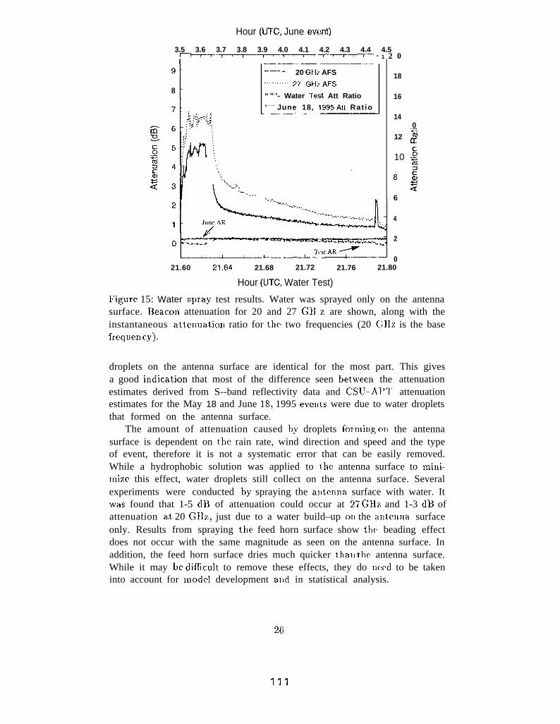
IPigure 15: Water spray test results. Water was sprayed only on the antennasurface. Beacon attenuation for 20 and 27 G]] z are shown, along with theinstantaneous attcnuaticm ratio for the two frequencies (20 C;IIZ is the basefrequcm cy).

droplets on the antenna surface are identical for the most part. This gives. . .

a good md]catlon that most of the difference seen between the attenuationestimates derived from S--band reflectivity data and CSU-Al’~’ attenuationestimates for the May 18 and June 18, 1995 events were due to water dropletsthat formed on the antenna surface.

The amount of attenuation caused by droplets fo]ming c)n the antennasurface is dependent on the rain rate, wind direction and speed and the typeof event, therefore it is not a systematic error that can be easily removed.While a hydrophobic solution was applied to the antenna surface to mini-]nize this effect, water droplets still collect on the antenna surface. Severalexperiments were conducted by spraying the alitenna surface with water. Itwas found that 1-5 dll of attenuation could occur at 27 GHz and 1-3 dll ofattenuation at 20 GHz, just due to a water build–up OIL the mltenna surfaceonly. Results from spraying the feed horn surface show the beading effectdoes not occur with the same magnitude as seen on the antenna surface. Inaddition, the feed horn surface dries much quicker than the antenna surface.While it may h difllcult to remove these effects, they do need to be takeninto account for model development and in statistical analysis.

26

111

5 Conclusions

Due to the high demand for satellite communications, already overused por-tions of the frecluency spectrum (C and Ku–ba]lds) are beco]]”ling even morecrowded. l’his necessitates looking at less crowded areas of the spectrumsuch as the Ka–band frequencies. TO study satellite communications atthese frequencies, NASA launched the Advanced Communications ‘l’echnol-ogy Satellite (ACTS). The ACTS is an experinlenta] satclliie being used toconduct communicaticm and propagation experiments using new Ka–bandtechnology. At Ka-- bancl, weather events can have an adverse affect on thesignal being propagated through the atmosphere. Therefore, propagationeffects at these frequencies must be studied. ‘J’his report has outlined theresearch that has been conducted at CSU durillg the first two years to meetthe ACTS experiment goals and further the understanding of K- band prop-agation effects.

The main goa~ of collstructing an attenuation data base for the B2 cli-matic zone at K–band frequencies was met by lnaintainin.g a well calibratedground propagation ternlirla~ and ensuri]lg the integrity of the data collectedand processed. Data were collected and preprocessed for the two year pe-riod of December 1, 1993 through November 30, 1995. A statistical analysisfor the CSU-APT data was presented in Section 2 and Appendix A. Theanalysis was done on a monthly and annual basis.

An attenuation model was developed to relate S-band radar reflectivityto Ka–band attenuation. Several case studies were presented to illustrate theattenuation model. They included a ve]y strong convective case, with knownmixed phase, that occurred on June 20, 1994, a second, weaker convectiveevent that occurred on May 18, 1995 and finally a stratiform event thatoccurred on June 18, 1995. Radar data, collected by the CSU - CHILL radar,for each of these events were used as inputs to the attenuation model. Verygood results were obtained for each case.

Finally to conclude, the ACTS prc)pagatioll experiment is an on-goingexperiment with two years of data collection completed, the third year inprogress and the possibility of a, fourth year. With the increased demandfrom industry to utilize the Ka-13and spectrum, the attenuation data beingcollected here, as well as at other sites, and its subsequent mlalysis will beinvaluable for the field of satellite com]nunications.

27

1 1 2