kefal, adnan and oterkus, erkan (2016) displacement and

Kefal, Adnan and Oterkus, Erkan (2016) Displacement and stress

monitoring of a Panamax containership using inverse finite element

method. Ocean Engineering, 119. pp. 16-29. ISSN 0029-8018 ,

http://dx.doi.org/10.1016/j.oceaneng.2016.04.025

This version is available at http://strathprints.strath.ac.uk/56240/

Strathprints is designed to allow users to access the research output of the University of

Strathclyde. Unless otherwise explicitly stated on the manuscript, Copyright © and Moral Rights

for the papers on this site are retained by the individual authors and/or other copyright owners.

Please check the manuscript for details of any other licences that may have been applied. You

may not engage in further distribution of the material for any profitmaking activities or any

commercial gain. You may freely distribute both the url (http://strathprints.strath.ac.uk/) and the

content of this paper for research or private study, educational, or not-for-profit purposes without

prior permission or charge.

Any correspondence concerning this service should be sent to the Strathprints administrator:

[email protected]

The Strathprints institutional repository (http://strathprints.strath.ac.uk) is a digital archive of University of Strathclyde research

outputs. It has been developed to disseminate open access research outputs, expose data about those outputs, and enable the

management and persistent access to Strathclyde's intellectual output.

http://strathprints.strath.ac.uk/

mailto:[email protected]

http://strathprints.strath.ac.uk/

1

Displacement and stress monitoring of a Panamax containership using inverse finite

element method

Adnan Kefal*, Erkan Oterkus**

* Department of Naval Architecture, Ocean and Marine Engineering University of Strathclyde

100 Montrose Street Glasgow G4 0LZ, United Kingdom

Phone: +44 (0)141 5484094

e-mail: [email protected]

** Department of Naval Architecture, Ocean and Marine Engineering University of Strathclyde

100 Montrose Street Glasgow G4 0LZ, United Kingdom

Phone: +44 (0)141 5483876

e-mail: [email protected]

Abstract: The inverse Finite Element Method (iFEM) is a revolutionary methodology for real-

time reconstruction of full-field structural displacements and stresses in plate and shell structures

that are instrumented by strain sensors. This inverse problem is essential for structural health

monitoring systems and commonly referred as ‘displacement and stress monitoring’ or ‘shape-

and stress-sensing’. In this study, displacement and stress monitoring of a Panamax containership

is performed based on the iFEM methodology. A simple, efficient, and practically useful four-

node quadrilateral inverse-shell element, iQS4, is used for the numerical implementation of the

iFEM algorithm. Hydrodynamic analysis of the containership is performed for beam sea waves

in order to calculate vertical and horizontal wave bending moments, and torsional wave moments

acting on parallel mid-body of the containership. Several direct FEM analyses of the parallel

mid-body are performed using the hydrodynamic wave bending and torsion moments. Then,

experimentally measured strains are simulated by strains obtained from high-fidelity finite

element solutions. After that, three different iFEM case studies of the parallel mid-body are

performed utilizing the simulated sensor strains. Finally, the effect of sensor locations and

number of sensors are assessed with respect to the solution accuracy.

Keywords: Displacement and Stress Monitoring, Structural Health Monitoring, Inverse Finite

Element Method (iFEM), Panamax Containership.

2

1. Introduction

Vessels are operated under challenging conditions because marine environment can cause

failure of the structure due to extreme or cyclic loadings, corrosion, and erosion. Structural

failure may lead to major accidents that may result in crew or passenger life loses, pollution of

the marine environment, and very expensive maintenance/repair costs. Therefore, it is necessary

to ensure safety, reliability, and integrity of ship structures for avoiding major accidents.

Moreover, the number of new vessels is increasing day-to-day. Therefore, new structural

designs, new construction techniques, and new materials are progressively being used in the

shipbuilding industry. As a result, it is necessary to increase knowledge about the on-site

structural performance not only for traditionally designed ships, but also for newly designed

ships.

Structural Health Monitoring (SHM) is an interdisciplinary procedure that (1) integrates

sensing systems to the structure, (2) processes the data collected from the sensing systems in

real-time, and (3) provides decisive real-time information from the structure about its global

and/or local structural state. Therefore, the necessities mentioned earlier and detailed structural

management of the ships including inspection, maintenance, and repair plans can only be

successfully accomplished if an application of SHM system is installed into the ships. In 1994,

the International Maritime Organization (IMO) originally recommended the utilization of hull

stress monitoring systems to facilitate the safe operation of ships. Then, the requirements for a

typical hull structural monitoring system are regulated by class societies including ABS (1995),

LR (2004), and DNV (2011). Recently, ABS (2015) has published a guide that discusses the

need for fitting of hull condition monitoring systems on all types and sizes of merchant vessels.

Besides, plenty of researchers considered the hull structural monitoring as an important case

study. For example, different types of hull structural monitoring systems are investigated for

various ship types (Van der Cammen 2008, Torkildsen et al. 2005, Andersson et al. 2011, Sielski

2012, Zhu and Frangopol 2013, Hageman et al. 2013, and Majewska et al. 2014). In particular,

Phelps and Morris (2013) presented a general review regarding the technical aspects of available

hull structural monitoring systems. However, most of the aforementioned SHM approaches don’t

take into account the advanced structural topologies and boundary conditions. Moreover, they

mostly require sufficiently accurate loading information even though it is not easy to estimate

3

dynamic loads of waves and winds due to the complexity and statistical feature of oceanographic

phenomena. Furthermore, some of them are not appropriate for use in real-time due to the time-

consuming analysis.

Real-time processing of the data obtained from a system composed of a network of strain

sensors is the key component of the SHM procedure for supplying trustworthy information about

the structural condition. In other words, real-time reconstruction of three-dimensional structural

displacements and stresses by utilizing discrete on-board strain measurements, known as

‘displacement and stress monitoring’ or ‘shape- and stress-sensing’, is the primary technology

for performing an accurate SHM. Apart from the SHM systems mentioned earlier, Tessler and

Spangler (2003, 2005) developed a powerful algorithm called inverse Finite Element Method

(iFEM) for the purpose of displacement and stress monitoring of engineering structures. In

contrast to other developed SHM methods, iFEM framework has a general applicability to any

type of structural topology and boundary conditions because using inverse beam, frame, plate,

and shell elements enables an effective discretization of the physical domain. The iFEM

algorithm minimizes a weighted-least-squares functional with respect to nodal displacements in

order to perform the shape-sensing of the structure. Since the iFEM weighted-least-squares

functional is defined by using only strain-displacement relationship, the iFEM methodology can

reconstruct the structural deformed shapes of the structure without prior knowledge of material

properties and loading information. Therefore, unlike other proposed SHM systems, stability and

accuracy of the shape-sensing results obtained through iFEM methodology is independent from

material properties of the structure and any type of static or dynamic loadings acting on the

structure. In fact, this special feature makes the iFEM methodology much more powerful than

the other SHM systems. Once the structural deformed shape is obtained, the full field strains can

be calculated from strain-displacement relationship. Then, full field stresses of the structure can

be evaluated by using full field strains and material properties of the structure. This stress

calculation not only allows iFEM methodology to perform stress-sensing of the structure, but

also allows real-time damage predictions if the full field structural stresses are converted to an

equivalent stress by using an appropriate failure criterion such as von Mises yield criterion.

Many different numerical and experimental iFEM studies have proved that the iFEM

framework is an accurate, robust, and fast shape- and stress-sensing algorithm. For example,

4

Tessler and Spangler (2004) developed a three-node inverse shell element (iMIN3) by using

lowest-order anisoparametric C0 continuous functions and adopting kinematic assumptions of the

first-order and shear-deformation theory. Tessler and Spangler (2004) numerically verified the

precision of iMIN3 element for performing iFEM analysis of plate/shell structures. Also, Quach

et al. (2005) and Vazquez et al. (2005) confirmed the robustness of the iMIN3 element by

conducting laboratory tests that uses experimentally measured real-time strain data. Moreover,

Tessler et al. (2012) enhanced iMIN3 element for displacement and stress monitoring of plate

and shell structures undergoing large displacements. Apart from iMIN3, Kefal et al. (2016) have

recently formulated a four-node quadrilateral inverse-shell element, iQS4, utilizing the kinematic

assumptions of the first-order and transverse-shear deformation theory. This new element

includes hierarchical drilling rotation degrees-of-freedom (DOF) and further extends the

practical usefulness of iFEM for shape-sensing analysis of large-scale structures. Kefal et al.

(2016) numerically verified the precision of the iQS4 element by the analysis of several

validation and demonstration problems. Furthermore, Cerracchio et al. (2010) and Gherlone et al.

(2011, 2012, 2014) formulated a robust inverse frame element that uses kinematic assumptions

of Timoshenko beam theory including stretching, bending, transverse-shear and torsion

deformation modes. They numerically and experimentally validated capability of their inverse

frame element by conducting several shape-sensing analyses of three-dimensional frame

structures undergoing static and/or damped harmonic excitations. Moreover, Cerracchio et al.

(2013, 2015a) has recently improved the original iFEM formulation of Tessler and Spangler

(2003, 2005) by adding the kinematic assumptions of recently developed Refined Zigzag Theory

(Tessler et al., 2009, 2010) in order to perform SHM of multi-layered composite and sandwich

structures. The application of iFEM methodology for SHM of future aerospace vehicles is

discussed by Tessler (2007) and Tessler et al. (2011). Likewise, another application of iFEM

algorithm to real-time displacement monitoring of a composite stiffened panel is presented by

Cerracchio et. al. (2015b). Apart from the aerospace applications, Kefal and Oterkus (2015)

performed shape-sensing of a longitudinally and transversely stiffened plate as a fundamental

application of the iFEM framework to SHM of marine structures. Similarly, Kefal and Oterkus

(2016) presented a more sophisticated application of iFEM to marine structures namely

displacement and stress monitoring of a chemical tanker based on iFEM algorithm. They

performed iFEM case studies when the chemical tanker is subjected to the head sea waves

5

because this phenomenon of ship advancing in waves can be very crucial for closed-decked ships

such as chemical tanker. However, for open-decked ships such as containerships, head sea wave

loads may be less important than beam sea wave loads due to torsional and warping stresses

induced by torsional moments. Since hull girder torsion loading on containerships represent a

major loading quantity particularly when combined with hull girder vertical and horizontal

bending loads, displacement and stresses monitoring of a containership floating in beam sea

waves should be investigated in addition to all proposed iFEM marine structure applications.

Hence, the main focus of this study is to demonstrate the application of the iFEM

methodology for monitoring multi-axial deformations and stresses of a Panamax containership

for the first time in the literature. For this purpose, the numerical implementation of the iFEM

algorithm is done using the simple, efficient, and practically useful iQS4 element developed by

Kefal et.al (2016). Hull form of a Panamax containership is designed performing several hull

surface transformations of S175 containership. A typical mid-ship section is designed for the

Panamax containership and the parallel mid-body of the containership is modelled using the

iQS4 element. The ‘smart methodology’ proposed by Kefal et al. (2015) is followed to determine

the optimum sensor locations for performing iFEM analyses of the parallel mid-body. First of all,

hydrodynamic analysis of the containership is performed for beam sea waves. As an output,

oscillatory pressures acting on the hydrodynamic panels, rigid body motions of the containership,

and hydrodynamic section forces including vertical and horizontal bending moments and

torsional moments are obtained. Secondly, several direct FEM analyses of the parallel mid-body

are performed using the hydrodynamic wave bending and torsion moments. Then,

experimentally measured strains are simulated by strains obtained from high-fidelity finite

element solutions. Thirdly, three different iFEM analyses of the parallel mid-body are performed

utilizing the simulated sensor strains obtained for three different cases. These are (1) pure

vertical bending case, (2) pure horizontal bending case and (3) pure torsion case. Finally, the

effect of sensor locations and number of sensors are assessed with respect to the solution

accuracy of each iFEM analysis.

6

2. Inverse finite element formulation for shells (Kefal et al., 2016)

2.1. Quadrilateral inverse-shell element

The four-node quadrilateral inverse-shell element (iQS4), developed by Kefal et al. (2016), is

adopted to demonstrate the iFEM formulation for shells. The iQS4 element has six displacement

DOF per node including a hierarchical drilling rotation (Fig. 1). As a result of the inclusion of

drilling rotations, the iQS4 element has two beneficial features: (1) singular solutions can be

simply avoided when modelling complex shell structures, (2) for membrane problems, iQS4

element has less tendency toward shear locking. In fact, these features make the iQS4 an

efficient and practically useful element.

First of all, a set of convenient coordinate frames of reference are defined to guarantee the

geometric uniqueness of the assembled shell structure. A local coordinate system ( , , )x y z serves

as the element frame of reference, with its origin (0,0,0) located at the centroid of mid-plane

quadrilateral. It is assumed that the shell element has a uniform thickness 2h , and that

,z h h defines the thickness coordinate (Fig. 1). Herein, displacement, strain, and stress

field of the iQS4 element is formulated using the local coordinate system. To assemble element

matrices into a global system of equations, suitable transformation matrices defining the local to

global transformations can easily be established with the element nodes referred to the global

coordinates ( , , )X Y Z . Details of how to allocate the local coordinate system at the centroid of

mid-plane quadrilateral and establish the transformation matrices defining the local to global

transformations are summarized in Appendix A.

The nodal DOF, consisting of positive x translations iu , positive y translations iv , and positive

clockwise drilling rotations zi , define the u and v membrane displacements as

4 4

1 1

( , ) i i i zi

i i

u x y u N u L

(1a)

4 4

1 1

( , ) i i i zi

i i

v x y v N v M

(1b)

7

The DOF of positive z translation iw and positive counter clockwise rotations around the x- and

y- axes, xi and yi , define the transverse displacement w and two bending rotations

x and y

by

4 4 4

1 1 1

( , ) i i i xi i yi

i i i

w x y w N w L M

(2a)

4

1

( , )x x i xi

i

x y N

(2b)

4

1

( , )y y i yi

i

x y N

(2c)

where iN is bilinear isoparametric shape functions, iL and iM are the anisoparametric shape

functions. These shape functions are analogous to four-node flat shell element described by Cook

(1994) and MIN4 (Mindlin-type, four-nodes) element provided by Tessler and Hughes (1983).

The three components of the displacement vector of any material point within the element can be

described as:

( , , )x x yu x y z u u z (3a)

( , , )y y xu x y z u v z (3b)

( , , )z zu x y z u w (3c)

where xu and yu are the in-plane displacements and zu is the transverse displacement

(deflection) across the uniform shell thickness.

For brevity, linear strain-displacement relations of linear elasticity are expressed in terms of

nodal displacement vector, eu , as

( ) ( )e e m e k e

b z z i = e u k u B u B u (4a)

( )e s e

s i = g u B u (4b)

with

T

b xx yy xy i (4c)

T

s xz yz i (4d)

8

and

1 2 3 4

Te e e e e u u u u u (4e)

with ( 1,2,3,4)T

e

i i i i xi yi ziu v w i u (4f)

where the matrices mB , kB , and sB contain derivatives of the shape functions. The explicit

forms of the shape functions iN , iL , and

iM , and mB , kB , and sB matrices are given in

Appendix B.

The membrane strains ( )ee u are associated with the stretching of the middle surface.

Therefore, mB matrix contains the derivatives of the shape functions associated with the

membrane behaviour. Furthermore, ( )ek u and ( )eg u are the bending curvatures and the

transverse shear strains, respectively. Hence, kB and sB matrices contain the corresponding

derivatives of shape functions used to define bending behaviour of the element. Note that the

plane-stress assumption 0zz within the theory implies that the transverse-normal strain zz

does not contribute to the strain energy.

2.2. Input data from in-situ strain sensors

Discrete in-situ strain measurements obtained from on-board sensors are crucial for the iFEM

methodology. Conventional strain rosettes or embedded fibre-optic sensor networks such as

Fibre Bragg Grating (FBG) sensors and Sensing Fibre Optic Cables can be used to collect large

amount of on-board strain data. With today’s technology, most of the strain sensors potentially

offer a number of advantages for installation as they are lightweight, high speed, and not affected

by electromagnetic interference and do not require re-calibration once installed. In order to

calculate membrane and bending section strains experimentally, the in-situ strain rosettes should

be located on top and bottom surfaces of the iQS4 element as shown in Fig. 2.

The experimentally measured (in-situ) membrane section strains i

e and curvatures i

k that

correspond to their analytic counterparts, ( )e ue and ( )k ue given by Eq. (4), can be determined

from the measured surface strains at n discrete locations ( , , )i i ix y h x ( 1,..., )i n located

9

within the element. These in-situ section strains are computed as follows (Tessler and Spangler,

2005)

1

2i i i

e i i (5a)

1

2i i i

h

k i i (5b)

where

T

i xx yy xy i i (5c)

and

T

i xx yy xy i i (5d)

are the measured surface strains, with the superscripts ‘+’ and ‘–’ denoting the quantities that

correspond to the top and bottom surface locations, respectively.

Although the experimentally measured surface strains can be used to compute the in-situ

membrane strains i

e and bending curvatures i

k , they cannot be directly used to calculate the in-

situ transverse shear strains i

g . A smoothing procedure, called the Smoothing Element Analysis

(Tessler et al. 1998, 1999), enables the first-order derivatives of i

k to be accurately computed

and subsequently used to obtain the transverse shear strains i

g . It is noted, however, that in the

deformation of thin shells, the contributions of i

g are much smaller compared to the bending

curvatures i

k . Since most of the marine structures are generally suitable to be modelled by using

thin shells, the i

g contributions can be safely omitted in the iFEM formulation.

2.3. Weighted least-squares functional of inverse finite element method

The inverse finite element method (iFEM) reconstructs the deformed shape of a discretized

structure by minimizing a weighted least-squares functional with respect to the nodal DOF of the

entire discretization. For an individual inverse element, this functional, ( )e

e u , accounts for the

membrane, bending and transverse shear deformations and is expressed according to Tessler et

al. (2011) by

10

2 2 2

( ) ( ) ( ) ( )e e e e

e e k gw w w u e u e k u k g u g (6a)

The squared norms expressed in Eq. (6a) can be written in the form of the normalized Euclidean

norms

22

1

1( ) ( )

e

ne e

i i

iA

dxdyn

e u e e u e (6b)

2

22

1

2( ) ( )

e

ne e

i i

iA

hdxdy

n

k u k k u k (6c)

22

1

1( ) ( )

e

ne e

i i

iA

dxdyn

g u g g u g (6d)

where eA represents the mid-plane area of the element. The weighting constants ew , kw , and gw

in Eq. (6a) are positive valued and are associated with the individual section strains. They control

the complete coherence between the analytic section strains and their experimentally measured

values. Their proper usage is especially critical for the problems involving relatively few

locations of strain gages. When every analytic section strain has a corresponding measured in-

situ value (i

e , i

k , and i

g ), the weighting constants are set as 1e k gw w w in Eqs. (6b-6d).

In the case of a missing in-situ strain component, the corresponding weighting constant is set

to be small, e.g., 510 , and Eqs. (6b-d) take on the reduced form

22( ) ( )

e

e e

A

dxdy e u e u with ( )ew (7a)

2 2 2( ) 2 ( )e

e e

A

h dxdy k u k u with ( )kw (7b)

22( ) ( )

e

e e

A

dxdy g u g u with ( )gw (7c)

where implementation of Eqs. (7) is performed on the component-by-component basis.

Furthermore, iFEM also permits the use of ‘strain-less’ inverse elements – the type of

elements that do not have any in-situ section-strain measurements. For these ‘strain-less’

elements, all squared norms in Eqs. (7) are multiplied by the small weighting constants

510e k gw w w . Therefore, an iFEM discretization can have very sparse measured strain

11

data, and yet the necessary interpolation connectivity can still be maintained between the

elements that have strain-sensor data.

By virtue of these assumptions, all strain compatibility relations are explicitly satisfied so that

Eq. (6a) can be minimized with respect to the nodal displacement DOF, giving rise to

( )0

ee e ee

e

u

k u fu

(8a)

or simply

e e ek u f (8b)

where ek is the element left-hand-side matrix, ef is the element right-hand-side vector that is a

function of the measured strain values, and eu is the nodal displacement vector of the element.

The element ek matrix can be explicitly written in terms of the mB , kB , and Bs matrices and

their corresponding weighting constants ew , kw , and gw , and is given by

22

e

T T Te m m k k s s

e k g

A

w w h w dxdy k B B B B B B (8c)

The ef vector is a function of the number of strain sensors within the element as well as the

measured section-strain values, and is given by

2

1

12

e

nT T T

e m k s

e i k i g i

iA

w w h w dxdyn

f B e B k B g (8d)

Once the element (local) matrix equations are established, the element contributions to the

global linear equation system of the discretized structure can be performed as

KU F (9a)

with

1

nelT

e e e

e

K T k T (9b)

1

nelT

e e

e

F T f (9c)

12

1

nelT

e e

e

U T u (9d)

where Te is the transformation matrix of the nodal DOF of an element from the local to the

global coordinate system (explicitly given in Appendix A), K is the global left-hand-side matrix

(symmetric matrix and independent of the measured strain values), U is the global nodal

displacement vector, F is the global right-hand-side vector (function of the measured strain

values), and the parameter nel stands for the total number of inverse finite elements.

The global left-hand-side matrix K includes the rigid body motion mode of the discretized

structure. Therefore, it is a singular matrix. By prescribing problem-specific displacement

boundary conditions, the resulting system of equations can be reduced from Eq. (9a) as

R R RK U F (10)

where RK is a positive definite matrix (always non-singular), and thus it is invertible. The

solution of Eq. (10) is very fast because the matrix RK remains unchanged for a given

distribution of strain sensors and its inverse should be calculated only once during the length of

the real time monitoring process. However, the right-hand-side vector FR is dependent on the

discrete surface strain data obtained from in-situ strain sensors. Hence, it needs to be updated

during any deformation cycle. The matrix–vector multiplication 1K FR R

gives rise to the

unknown DOF vector UR , which provides the deformed structural shape at any real-time.

Finally, the global displacement response can be assessed by computing the total displacement as

2 2 2

TU U V W (11)

where U , V , and W are the translations (displacements) along the global X-, Y-, and Z-axes,

respectively.

By using the evaluated displacement values, the continuous strain field throughout the

structure can be obtained. Furthermore, the constitutive relationship between stress and strain

will allow determination of stress distribution. For instance, the constitutive relationship for

isotropic materials can be defined based on the plane-stress assumption 0zz as

m e k e

b b b b bz j D i D B u D B u (12a)

13

s e

s s s s j D i D B u (12b)

where

T

b xx yy xy j (12c)

T

s xz yz j (12d)

and

2

1 0

1 01

0 0 1 2

b

E

D (12e)

1 0

0 12 1s

E

D

(12f)

are the reduced form of general isotropic stiffness matrix, with E and denoting elastic

modulus and Poisson’s ratio of the isotropic material, respectively. Once the stress components

at any point inside the iQS4 element domain are calculated using Eqs. (12), transformation of the

stress components from the local to the global coordinate system can be performed as

T ej T j T (13a)

where

0

xx xy xz

e

xy yy yz

xz yz

j

(13b)

XX XY XZ

XY YY YZ

XZ YZ ZZ

j

(13c)

and T is the stress transformation matrix of an element from the local to the global coordinate

system which is explicitly given in Appendix A. Finally, a suitable failure criterion can be used

for damage detection as part of the SHM process. For instance, three-dimensional global stress

components can be converted to an equivalent stress using the von Mises failure criterion as

14

2 2 2 2 2 216

2VM XX YY XX ZZ YY ZZ XY XZ YZ

(14)

3. iFEM analysis of a Panamax containership

3.1. Panamax containership model

The body plan of S175 containership, given by Wu and Hermundstad (2002), is used as a

‘parent ship hull form’ in order to design a Panamax containership. Firstly, the hull form of the

Panamax containership is obtained performing several hull form transformations of the S175

containership. These transformations are (1) linearly scaling based upon the characteristic

breadth, and (2) linearly lengthening the parallel mid-body. Once the design of the hull form is

completed, a typical mid-ship section is also designed for the Panamax containership. Isometric

view of the hull surface below the draft waterline and mid-ship section drawings are depicted in

Figs. 3 and 4, respectively.

For clarity, only one global Cartesian coordinate system ( , , )X Y Z serves as containership

frame of reference, with its origin (0,0,0) located at the still waterline and aligned vertically

with the ship’s centre of gravity. The X-, Y-, and Z-axes of the coordinate system point out the

bow, portside, and opposite direction of gravity, respectively. According to the global coordinate

system, when the containership is loaded at its design draft, the containership has the general

particulars as listed in Table 1.

Parallel mid-body of the containership is composed of three full and two half cargo holds and

is defined over the domain m[ 51.6 , 51.6 ]mX . Each ends of the cargo hold are separated

with watertight bulkheads and each cargo hold is equally subdivided into two cargo

compartments with a non-watertight bulkhead. Each cargo compartment has longitudinal space

of 12.48 m because they are designed for stowing 2x20 foot long containers. During the design

of the containership, longitudinal frame spacing methodology is adopted and each cargo

compartment is supported with three transverse frames. Moreover, both watertight and non-

watertight transverse bulkheads have length of 1.56 m and each bulkhead is supported with a

transverse frame at both ends. For simplicity, all the structural components including plates,

stiffeners, and transverse frames have been designed to have the uniform thickness of 30 mm and

they are made of steel having elastic modulus of E=210 GPa and Poisson’s ratio of Ȟ=0.3. In

15

order to represent the complexity of the structure more clearly, an isometric view of the parallel

mid-body is illustrated in Fig. 5.

3.2. Hydrodynamic-FEM analysis of the containership

In this study, the above stated parallel mid-body is analysed using the iFEM/iQS4

methodology to monitor the multi-axial deformations and stresses of the Panamax containership.

For each iFEM case study, optimum strain-sensor locations are determined utilizing ‘the smart

system/methodology’ proposed by Kefal et. al. (2015). Firstly, hydrodynamic loads acting on the

containership is calculated performing a hydrodynamic analysis. Secondly, an accurate reference

solution is established performing a direct FEM analysis. Then, the FEM deflections and

rotations are used to compute the simulated sensor strains. Finally, the iFEM analysis of the

parallel mid-body is performed using the simulated sensor strains. In-house hydrodynamic and

FEM codes developed by Kefal and Oterkus (2014) are used for the hydrodynamic-FEM

analysis.

The total weight of the containership is distributed along the length between perpendiculars as

depicted in Fig. 6. At this loading condition, the containership is assumed to float with zero

forward speed in beam sea waves. Using a full hydrodynamic model consisted of 4,912 flat

quadrilateral panels, the hydrodynamic analysis is performed. As a result, six DOF motions and

hydrodynamic pressures of the containership are obtained for unit wave amplitude and wave

frequencies ranging from 0.05 rad/s to 1.2 rad/s. The nonzero rigid body motion amplitudes,

namely sway, heave, and roll motions, are presented in Figs. 7 and 8, respectively.

At any section along the length, hydrodynamic section forces can be calculated using the six

DOF motions, the hydrodynamic pressures, and the total weight distribution. For open-decked

ships such as containerships, beam sea wave loads have a great impact on the strength of the

structure due to torsional and warping stresses induced by torsional moments. As can be seen

from Fig. 8, the roll motion amplitude significantly increases between wave frequencies of 0.2

rad/s and 0.4 rad/s. This result clearly demonstrates the wave frequency interval where the

torsional wave moments become the most critical loading component. Therefore, vertical and

horizontal wave bending moments, My and Mz, and torsional wave moments, Mx, at section

16

X=0 m are compared between the wave frequencies ranging from 0.2 rad/s to 0.4 rad/s as

depicted in Fig. 9.

As can be seen from Fig. 9, 0.31 rad/s is the most critical wave frequency for performing the

structural analysis, so that vertical and horizontal wave bending moments, My=20686 kNm/m

and Mz=23261 kNm/m, respectively, and torsional wave moment, Mx=18446 kNm/m, at 0.31

rad/s, are chosen as load input for the following direct FEM analysis. For clarity, total

hydrodynamic pressures P due to the oscillation at wave frequency of 0.31 rad/s are plotted over

the underwater panels of the containership as depicted in Fig. 10.

Structural analysis of the parallel mid-body is performed for three different loading cases.

They are (1) pure vertical bending case, (2) pure horizontal bending case and (3) pure torsion

case. For each loading case, the suitable moment obtained from hydrodynamic analysis is

uniformly applied along the length of the parallel mid-body. The resultant deformations due to

these three loading scenarios may be symmetric/antisymmetric with respect to XZ- and/or YZ-

planes. Moreover, geometry of the parallel mid-body is symmetric with respect to both XZ- and

YZ-planes. Therefore, only one-fourth of the mid-body is modelled instead of modelling the

entire mid-body. The translations along the normal axis and the rotations around the in-plane

axes are constrained for symmetry boundary condition, while the rotation around the normal axis

and the translations along the in-plane axes are constrained for anti-symmetry boundary

condition. For each loading case, the boundary conditions (BC) imposed to XZ- and YZ-planes

are listed in Table 2. Once the boundary conditions are applied to the FEM model, an accurate

reference solution is established performing a convergence study. The most refined mesh

consists of 246,484 shell elements, possessing 1,428,738 DOF. After the execution of direct

FEM analysis for each loading case, experimentally measured strains, i

i and i

i , are simulated

by strains obtained from the FEM analyses.

3.3. iFEM case studies of the containership

Three different iFEM analyses of the parallel mid-body are performed utilizing the simulated

sensor strains obtained for pure vertical bending case, pure horizontal bending case, and pure

torsion case, respectively. A different strain-rosette network is used for each iFEM analysis of

the mid-body. The resulting deformations of the mid-body exhibit both stretching and bending

17

response due to the complexity of the structural topology. Hence, the strain-rosettes have to be

placed on both the top and bottom surfaces of the plates. To take the advantage of the symmetry

and remain consistent with the above stated boundary conditions, only one-fourth of parallel

mid-body is discretised using iQS4 elements in the following iFEM analyses. Moreover, the hull

structure is made up with thin shells so the weighting constants for transverse shear strains are

set as 510gw in the following iFEM analyses.

In the first case study, i.e. pure vertical bending case, the iQS4 model of the parallel mid-body

has 15,318 elements with top- and bottom-surface strain rosettes located within 327 select

elements as shown in Figs. 11 and 12. For an iQS4 element which has no in-situ strain

components, the corresponding weighting coefficients are set to 10-5

.

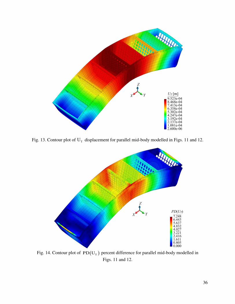
In Fig. 13, the contour plot for the TU displacement is depicted for the first iFEM analysis.

Although only one-fourth of the mid-body is analysed using the iQS4 mesh presented in Figs. 11

and 12, the results are illustrated using an iQS4 mesh corresponds to the entire parallel mid-body

for a better visualization of the deformed shape. Remarkably, the deformed shape of the mid-

body confirms the pure vertical bending of the structure (Fig. 13). To investigate the accuracy of

iFEM predictions for the TU displacement, the percent difference (PD) between iFEM and direct

FEM results for TU displacement can be computed for each node i as

, ,

,max

100%

iFEM FEM

T i T i

T FEM

T

U UPD U

U

(15)

where ,

iFEM

T iU is iFEM prediction for the TU displacement at node i , ,

FEM

T iU is direct FEM

prediction for the TU displacement at node i , and ,max

FEM

TU is direct FEM prediction of the

maximum TU displacement. In Fig. 14, contour plot of TPD U is shown for the first iFEM

analysis. As can be seen from Fig. 14, the maximum TPD U is equal to 7.248% and the

maximum TPD U is located at the node where the maximum TU displacement is occurred

(Fig. 13). Therefore, this result clearly demonstrates the superior accuracy of the iFEM solutions

for displacement monitoring.

18

Once the structural deformed shape is obtained, the von Mises stresses, VM , on the top

surfaces of the shells are calculated. In Fig. 15, the contour plot for the VM stress is presented

for the first iFEM analysis. Moreover, the accuracy of iFEM predictions for the VM stress is

examined by calculating the percent difference between iFEM and direct FEM predictions for

VM stress at each node i as

, ,

,max

100%

iFEM FEM

VM i VM i

VM FEM

VM

PD

(16)

where ,

iFEM

VM i is iFEM prediction for the VM stress at node i , ,

FEM

VM i is direct FEM prediction for

the VM stress at node i , and ,max

FEM

VM is direct FEM prediction of the maximum VM stress. In

Fig. 16, contour plot of VMPD is shown for the first iFEM analysis. The maximum

VMPD is equal to 12.569% and its location is identical to the location of the node where the

maximum VM stress is occurred (Figs. 15 and 16). Therefore, this result confirms superior

precision of the iFEM solutions for stress monitoring. These results also confirm the strain-

sensor locations depicted in Figs. 11 and 12 are the optimum locations for performing an

accurate shape- and stress-sensing of the Panamax containership subjected to vertical wave

bending moment.

In the second case study, i.e. pure horizontal bending case, the iQS4 model of the parallel

mid-body has 15,318 elements with top- and bottom-surface strain rosettes located within 413

select elements as shown in Figs. 17 and 18. For an iQS4 element which has no in-situ strain

components, the corresponding weighting coefficients are set to 10-5

.

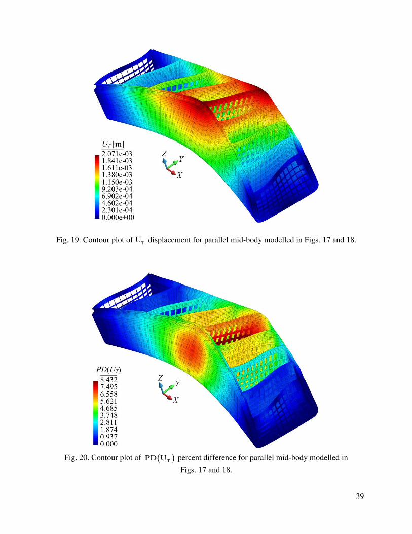
In Fig. 19, the contour plot for the TU displacement is demonstrated for the second iFEM

analysis. Similar to the first iFEM case study, a better visualization of the deformed shape is

achieved using an iQS4 mesh corresponds to the entire parallel mid-body. As can be seen from

the Fig. 19, the deformed shape of the mid-body is identical to the pure horizontal bending of the

structure. To demonstrate the accuracy of iFEM predictions for the TU displacement, contour

plot of TPD U for the second iFEM analysis is shown in Fig. 20. According to Figs. 19 and

20, TPD U is approximately equal to 5.5% at the location where the maximum TU

19

displacement is occurred. Hence, this result clearly demonstrates remarkable precision of the

iFEM solutions for shape-sensing.

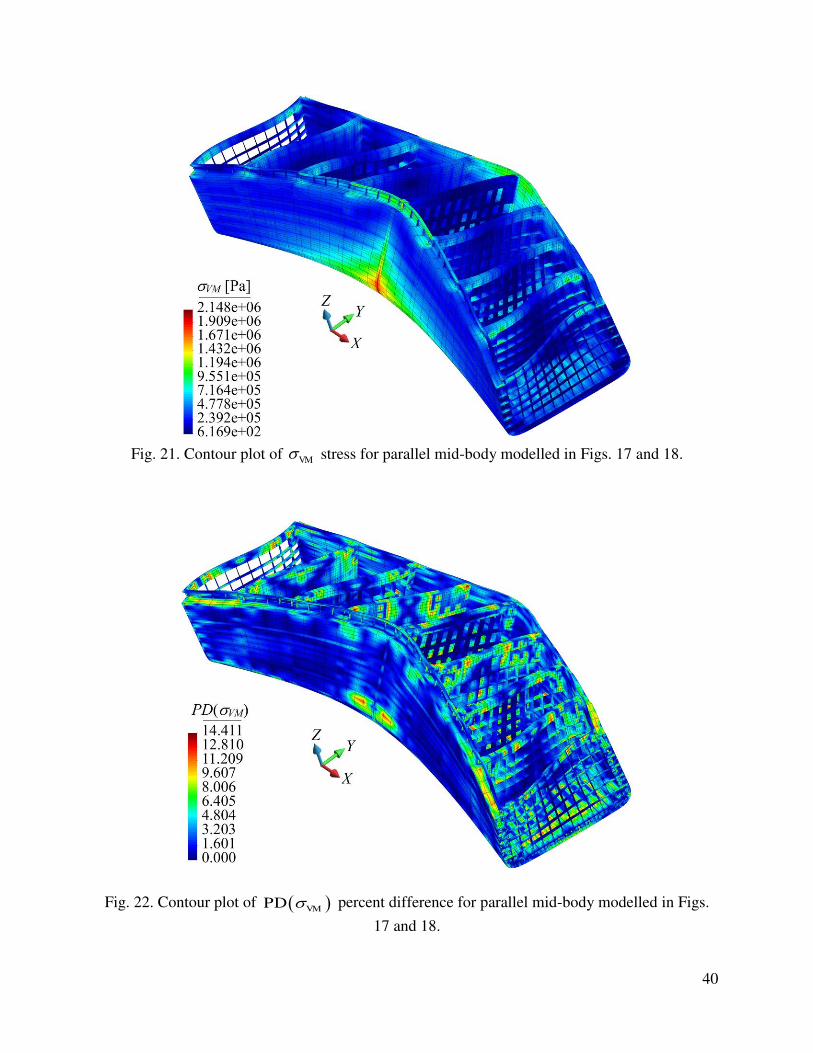
In Fig. 21, the contour plot for the VM stress calculated at the top surfaces of the shells is

presented for the second iFEM case study. Also, the accuracy of iFEM predictions for the VM

stress is examined by presenting contour plot of VMPD as shown in Fig. 22. As can be seen

from the Figs. 21 and 22, VMPD is around 8% at the location where the maximum VM

stress is occurred. Consequently, this result confirms high precision of the iFEM solutions for

stress-sensing. Furthermore, these results verify that the strain-sensor locations presented in Figs.

17 and 18 are the optimum locations for performing a precise displacement and stress monitoring

of the Panamax containership exposed to horizontal wave bending moment.

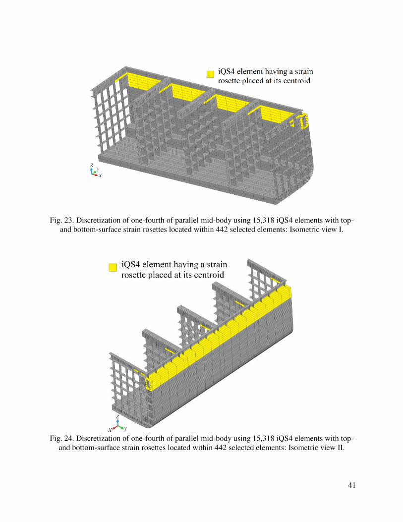
In the third case study, i.e. pure torsion case, the iQS4 model of the parallel mid-body has

15,318 elements with top- and bottom-surface strain rosettes located within 442 select elements

as shown in Figs. 23 and 24. For an iQS4 element which has no in-situ strain components, the

corresponding weighting coefficients are set to 10-5

.

In Fig. 25, the contour plot for the TU displacement is demonstrated for the third iFEM

analysis. An iQS4 mesh that represents the entire parallel mid-body is utilized for a better

visualization of the deformed shape. As can be seen from Fig. 25, the deformed shape of the

mid-body exhibits the pure torsion of the structure. According to Figs. 13, 19, and 25, the

maximum TU displacement induced due by torsional moment is much larger than the maximum

TU displacement caused due to vertical and horizontal bending moments. This result proofs the

significance of hull girder torsion loading on containerships floating in beam sea waves. In Fig.

26, contour plot of TPD U is depicted in order to investigate the accuracy of iFEM predictions

for the TU displacement found in the third iFEM case study. As can be seen from Figs. 25 and

26, TPD U is approximately equal to 7.1% at the location where the maximum TU

displacement is occurred. Hence, this result clearly indicates the significant precision of the

iFEM solutions for displacement monitoring.

20

In Fig. 27, the contour plot for the VM stress calculated at the top surfaces of the shells is

presented for the third iFEM case study. Additionally, in order to examine VM stress found in

the third iFEM case study, contour plot of VMPD is shown in Fig. 28. According to Figs. 27

and 28, VMPD is approximately 10.7% at the location where the maximum VM stress is

occurred. Hence, this result proofs superior precision of the iFEM solutions for stress

monitoring. These results also validate that the strain-sensor locations demonstrated in Figs. 23

and 24 are the optimum locations for performing a precise shape- and stress-sensing of the

Panamax containership subjected to torsional wave moment. According to the results found in

the three different iFEM case studies, it can be concluded that iFEM is a superior, powerful, and

innovative technology for the structural health monitoring of marine structures.

4. Concluding remarks

Displacement and stress monitoring of a Panamax containership is accomplished based on

iFEM methodology. The iFEM algorithm reconstructs the full-field displacements, strains, and

stresses of a structure from discrete in-situ strain measurements. The iFEM formulation is based

on a least-squares variational principle originally developed by Tessler and Spangler (2005).

Herein, a recently developed four-node quadrilateral inverse-shell element (iQS4) is utilized for

performing the shape- and stress-sensing of the containership. The parallel mid-body of the

containership is modelled using iQS4 elements as a representative of the global structural model.

Firstly, the hydrodynamic analysis of the Panamax containership is performed for the beam sea

waves. Secondly, the direct FEM analysis of the mid-body is performed using the hydrodynamic

wave bending and torsion moments as input. Then, the FEM deflections and rotations are used to

compute the simulated sensor strains. Thirdly, three different iFEM analyses of the parallel mid-

body are performed utilizing the simulated sensor strains obtained for three different cases.

These are (1) pure vertical bending case, (2) pure horizontal bending case and (3) pure torsion

case. Based on the same iQS4 mesh, a different network of strain-sensors is proposed for each

iFEM analysis. Then, the deformed shape and von Mises stresses of the containership are

reconstructed using in-situ strain data obtained from each proposed network of strain-sensors.

According to the accuracy of the displacement and stress results, the optimum strain-sensor

locations are identified and clearly demonstrated for each iFEM case study. Hence, the numerical

21

results confirmed the robustness of the iFEM methodology for monitoring multi-axial

deformations and stresses of a Panamax containership floating in beam sea waves.

22

Appendix A

The global coordinates of the iQS4 element nodes are given as

( 1,2,3,4)T

i i i iX Y Z i X (A.1)

Each edge length, id , and global coordinates of each edge mid-point, ic , can be calculated as

( 1,2,3,4; 2,3,4,1)

2

i j i

j i

i

d

i j

X X

X Xc

(A.2)

Using Eq. (A2), global coordinates of mid-plane quadrilateral centroid can be defined as

4

1

4

1

k k

k

k

k

d

d

c

C

(A.3)

Unit normal vector to the mid-plane quadrilateral, n , and unit vectors along local y- and x- axis,

p and l , can respectively be computed as:

A B

nA B

(A.4a)

A B

pA B

(A.4b)

l p n (A.4c)

where

3 1 A X X (A.4d)

4 2 B X X (A.4e)

are diagonal vectors, with A pointing out from node-1 to node-3, whereas B pointing out from

node-2 to node-4. Using Eq. (A1), Eq. (A3), and Eqs. (A4b-c), local coordinates of the iQS4

element nodes can be determined as

23

1,2,3,4i i

i i

xi

y

X C l

X C p (A.5)

With the unit vectors n , p , and l , given in Eqs.(4a-c), the transformation matrix of the nodal

DOF of an element from the local to the global coordinate system can be defined as

0 0 0 0 0 0 0

0 0 0 0 0 0 0

0 0 0 0 0 0 0

0 0 0 0 0 0 0

0 0 0 0 0 0 0

0 0 0 0 0 0 0

0 0 0 0 0 0 0

0 0 0 0 0 0 0

e

T

T

T

TT

T

T

T

T (A.6a)

where

TT T T T l p n

(A.6b)

is the stress transformation matrix from the local to the global coordinate system.

24

Appendix B

The shape functions iN , iL , and

iM , which are used to describe both membrane and bending

capability of the iQS4 element as given in Eqs. (1a-b) and Eqs. (2a-c), are respectively defined as

1

(1 )(1 )

4

s tN

(B.1)

2

(1 )(1 )

4

s tN

(B.2)

3

(1 )(1 )

4

s tN

(B.3)

4

(1 )(1 )

4

s tN

(B.4)

2

5

(1 )(1 )

16

s tN

(B.5)

2

6

(1 )(1 )

16

s tN

(B.6)

2

7

(1 )(1 )

16

s tN

(B.7)

2

8

(1 )(1 )

16

s tN

(B.8)

and

1 14 8 21 5L y N y N (B.9)

2 21 5 32 6L y N y N (B.10)

3 32 6 43 7L y N y N (B.11)

4 43 7 14 8L y N y N (B.12)

1 41 8 12 5M x N x N (B.13)

2 12 5 23 6M x N x N (B.14)

3 23 6 34 7M x N x N (B.15)

4 34 7 41 8M x N x N (B.16)

Note that ijx and

ijy can be expressed in terms of local coordinates of iQS4 element as

25

( 1,2,3,4; 1,2,3,4)ij i j

ij i j

x x xi j

y y y

(B.17)

and the parent space coordinates are defined as , 1, 1s t .

The derivatives of shape functions mB , kB , sB which are given in Eqs. (4a-b) are defined as

1 2 3 4

m m m m m B B B B B (B.18)

1 2 3 4

k k k k k B B B B B (B.19)

1 2 3 4

s s s s s B B B B B (B.20)

where

, ,

,y ,

,y , ,y ,

,

,y

,x ,y

, , ,

,y ,y ,y

0 0 0 0

0 0 0 0

0 0 0

0 0 0 0 0

0 0 0 0 0 ( 1,2,3,4)

0 0 0 0

0 0 0

0 0 0

i x i x

m

i i i x

i i x i i x

i x

k

i i

i i

i x i x i x is

i

i i i i

N L

N M

N N L M

N

N i

N N

N L M N

N L N M

B

B

B

(B.21)

26

References

American Bureau of Shipping. (1995). Guide for Hull Condition Monitoring Systems.

American Bureau of Shipping. (2015). Guide for Hull Condition Monitoring Systems.

Andersson, S., Haller, K., Hellbratt, S. E., & Hedberg, C. (2011). Damage monitoring of ship

FRP during exposure to explosion impacts. In Proc. 18th Inter. Conf. Composite Materials, Jeju

Island, Korea.

Cerracchio, P., Gherlone, M., Mattone, M., Di Sciuva, M., & Tessler, A. (2010). Shape sensing

of three-dimensional frame structures using the inverse finite element method. In: Proceedings of

5th European Workshop on Structural Health Monitoring, Sorrento, Italy.

Cerracchio, P., Gherlone, M., Di Sciuva, M., & Tessler, A. (2013). Shape and Stress Sensing of

Multilayered Composite and Sandwich Structures Using an Inverse Finite Element Method. In:

Proceedings of V International Conference on Computational Methods for Coupled Problems in

Science and Engineering, Ibiza, Spain.

Cerracchio, P., Gherlone, M., Di Sciuva, M., & Tessler, A. (2015a). A novel approach for

displacement and stress monitoring of sandwich structures based on the inverse Finite Element

Method. Composite Structures, 127, 69-76.

Cerracchio, P., Gherlone, M., & Tessler A. (2015b). Real-time displacement monitoring of a

composite stiffened panel subjected to mechanical and thermal loads. Meccanica, 50, 2487-2496.

Cook, R. D. (1994). Four-node ‘flat’ shell element: drilling degrees of freedom, membrane-

bending coupling, warped geometry, and behaviour. Computers and Structures, 50(4), 549-555.

Det Norske Veritas, Hull Monitoring Systems. (2011). DNV Rules for Classification of Ships,

Part 6, Chapter 11.

Gherlone, M., Cerracchio, P., Mattone, M., Di Sciuva, M., & Tessler, A. (2011). Beam shape

sensing using inverse finite element method: theory and experimental validation. In: Proceeding

of 8th International Workshop on Structural Health Monitoring, Stanford, CA

27

Gherlone, M., Cerracchio, P., Mattone, M., Di Sciuva, M., & Tessler, A. (2012). Shape sensing

of 3D frame structures using an inverse Finite Element Method. International Journal of Solids

and Structures, 49(22), 3100-3112.

Gherlone, M., Cerracchio, P., Mattone, M., Di Sciuva, M., & Tessler, A. (2014). An inverse

Finite Element Method for beam shape sensing: theoretical framework and experimental

validation. Smart Materials and Structures, 23(4), 045027.

Hageman, R., Aalbetrs, P., Shaik, M., & Van den Boom, H. (2013). Development of an Advisory

Hull Fatigue Monitoring System. In: Proceedings of SNAME Annual Meeting & Expo & Ship

Production Symposium, Bellevue, WA.

Kefal, A., & Oterkus, E. (2014). D3.3 (WP3) – Hydrodynamic and structural analysis. Public

Deliverable, The INCASS Project (FP7/2007-2013 grant agreement no 605200).

Kefal, A., & Oterkus, E. (2015). Structural Health Monitoring of marine structures by using

inverse Finite Element Method. Analysis and Design of Marine Structures V, 341-349.

Kefal, A., Hizir, O., & Oterkus, E. (2015). A smart system to determine sensor locations for

structural health monitoring of ship structures. In: Proceedings of 9th International Workshop on

Ship and Marine Hydrodynamics, Glasgow, UK, 2015.

Kefal, A., & Oterkus, E. (2016). Displacement and stress monitoring of a chemical tanker based

on inverse finite element method. Ocean Engineering, 112, 33-46.

Kefal, A., Oterkus, E., Tessler, A., & Spangler, J.L. (2016). A Quadrilateral Inverse-Shell

Element with Drilling Degrees of Freedom for Shape Sensing and Structural Health Monitoring.

Engineering Science and Technology, an International Journal, In Press.

http://dx.doi.org/10.1016/j.jestch.2016.03.006.

Lloyds Register. (2004). ShipRight Ship Event Analysis.

Majewska, K., Mieloszyk, M., Ostachowicz, W., & Król, A. (2014). Experimental method of

strain/stress measurements on tall sailing ships using Fibre Bragg Grating sensors. Applied

Ocean Research, 47, 270-283.

28

Phelps, B., & Morris, B. (2013). Review of Hull Structural Monitoring Systems for Navy Ships

(No. DSTO-TR-2818). Defense Science and Technology Organization Victoria (Australia)

Maritime Platforms Div.

Quach, C.C., Vazquez, S.L., Tessler, A., Moore, J.P., Cooper, E.G., & Spangler, J.L. (2005).

Structural anomaly detection using fiber optic sensors and inverse finite element method. In:

Proceedings of AIAA Guidance, Navigation, and Control Conference and Exhibit, San

Francisco, California.

Sielski, R. A. (2012). Ship structural health monitoring research at the Office of Naval Research.

JOM, 64(7), 823-827.

Tessler, A., & Hughes, T. J. (1983). An improved treatment of transverse shear in the Mindlin-

type four-node quadrilateral element. Computer Methods in Applied Mechanics and

Engineering, 39(3), 311-335.

Tessler, A., Riggs, H. R., Freese, C. E., & Cook, G. M. (1998). An improved variational method

for finite element stress recovery and a posteriori error estimation. Computer Methods in Applied

Mechanics and Engineering, 155(1), 15-30.

Tessler, A., Riggs, H. R., & Dambach, M. (1999). A novel four-node quadrilateral smoothing

element for stress enhancement and error estimation. International Journal for Numerical

Methods in Engineering, 44(10), 1527-1541.

Tessler, A., & Spangler, J.L. (2003). A variational principle for reconstruction of elastic

deformation of shear deformable plates and shells, NASA TM-2003-212445.

Tessler, A., & Spangler, J.L. (2004). Inverse FEM for full-field reconstruction of elastic

deformations in shear deformable plates and shells. In: Proceedings of 2nd European Work-shop

on Structural Health Monitoring, Munich, Germany.

Tessler, A., & Spangler, J. L. (2005). A least-squares variational method for full-field

reconstruction of elastic deformations in shear-deformable plates and shells. Computer Methods

in Applied Mechanics and Engineering, 194(2), 327-339.

Tessler, A. (2007). Structural Analysis Methods for Structural Health Management of Future

Aerospace Vehicles. Key Engineering Materials, 347, 57-66.

29

Tessler, A., Di Sciuva, M., & Gherlone, M. (2009). A refined zigzag beam theory for composite

and sandwich beams. Journal of Composite Materials, 43, 1051–1081.

Tessler, A., Di Sciuva, M., & Gherlone, M. (2010). A consistent refinement of first-order shear

deformation theory for laminated composite and sandwich plates using improved zigzag

kinematics. Journal of Mechanics of Materials and Structures, 5(2), 341-367.

Tessler, A., Spangler, J. L., Gherlone, M., Mattone, M., & Di Sciuva, M. (2011). Real-Time

characterization of aerospace structures using on-board strain measurement technologies and

inverse finite element method. In: Proceedings of the 8th International Workshop on Structural

Health Monitoring, Stanford, CA.

Tessler, A., Spangler, J. L., Gherlone M., Mattone M., & Di Sciuva, M. (2012). Deformed shape

and stress reconstruction in plate and shell structures undergoing large displacements:

application of inverse finite element method using fiber bragg grating strains. In: Proceedings of

10th World Congress on Computational Mechanics, Sao Paulo, Brazil.

Torkildsen, H. E., Grovlen, A., Skaugen, A., Wang, G., Jensen, A. E., Pran, K., & Sagvolden, G.

(2005). Development and applications of full-scale ship hull health monitoring systems for the

Royal Norwegian Navy. Norwegian Defence Research Establishment Kjeller.

Van der Cammen, J. J. (2008). Fatigue prediction and response monitoring on a FPSO. TU Delft,

Delft University of Technology.

Vazquez, S.L., Tessler, A., Quach, C.C., Cooper, E.G., Parks, J., & Spangler J.L. (2005).

Structural health monitoring using high-density fiber optic strain sensor and inverse finite

element methods, NASA TM-2005-213761.

Wu, M., & Hermundstad, O. A. (2002). Time-domain simulation of wave-induced nonlinear

motions and loads and its applications in ship design. Marine Structures, 15(6), 561-597.

Zhu, B., & Frangopol, D. M. (2013). Incorporation of structural health monitoring data on load

effects in the reliability and redundancy assessment of ship cross-sections using Bayesian

updating. Structural Health Monitoring, 12(4), 377-392.

30

Fig. 1. (a) Four-node quadrilateral inverse shell element, iQS4, depicted within global (X, Y, Z)

and local (x, y, z) frames of reference; (b) Nodal degrees-of-freedom corresponding to local

(element) coordinates (x, y, z).

Fig. 2. Discrete surface strains measured by strain rosettes within iQS4 element at

, ,i i ix y h x locations.

31

Fig. 3. Isometric view of the hull surface below draft waterline.

Fig. 4. Mid-ship section of the Panamax containership.

32

Fig. 5. Parallel mid-body of the Panamax containership.

Fig. 6. Total weight distribution of the containership.

33

Fig. 7. Sway and heave motion amplitudes.

Fig. 8. Roll motion amplitudes.

34

Fig. 9. Wave vertical and horizontal bending and torsional moments.

Fig. 10. Contour plot of total hydrodynamic pressure P at wave frequency of 0.31 rad/s.

35

Fig. 11. Discretization of one-fourth of parallel mid-body using 15,318 iQS4 elements with top-

and bottom-surface strain rosettes located within 327 selected elements: Isometric view I.


and bottom-surface strain rosettes located within 327 selected elements: Isometric view II.

36

Fig. 13. Contour plot of TU displacement for parallel mid-body modelled in Figs. 11 and 12.

Fig. 14. Contour plot of TPD U percent difference for parallel mid-body modelled in

Figs. 11 and 12.

37

Fig. 15. Contour plot of VM stress for parallel mid-body modelled in Figs. 11 and 12.

Fig. 16. Contour plot of VMPD percent difference for parallel mid-body modelled in Figs.

11 and 12.

38





39



Figs. 17 and 18.

40



17 and 18.

41





42



Figs. 23 and 24.

43



23 and 24.

44

Table 1. General particulars of Panamax containership.

General particular Value Unit

Length between perpendiculars 291 m

Breadth (moulded) 32.3 m

Depth (moulded) 19.9 m

Design draft (moulded) 12.1 m

Block coefficient 0.73 m3/m

3

Displacement (at design draft) 85190.5 tonnes

Vertical centre of gravity (from baseline) 12.1 m

Vertical centre of buoyancy (from baseline) 6.4 m

Longitudinal centre of gravity (from aft perpendicular) 141.2 m

Longitudinal centre of buoyancy (from aft perpendicular) 141.2 m

Radius of gyration around X-axis 10.834 m

Radius of gyration around Y-axis 74.105 m

Radius of gyration around Z-axis 74.105 m

Radius of gyration for roll-yaw product of inertia 0 m

Table 2. Constraint boundary conditions.

Loading case XZ-plane YZ-plane

Pure vertical bending case Symmetry BC Symmetry BC

Pure horizontal bending case Anti-symmetry BC Symmetry BC

Pure torsion case Anti-symmetry BC Anti-symmetry BC

kefal, adnan and oterkus, erkan (2016) displacement and

Documents