keller 2011

2642 IEEE TRANSACTIONS ON SIGNAL PROCESSING, VOL. 59, NO. 6, JUNE 2011

A Diffusion Approach to Network LocalizationYosi Keller and Yaniv Gur

Abstract—The localization of nodes on a network is a challengingresearch topic. It arises in a variety of applications such as com-munications and sensor network analysis. We propose a computa-tional approach to recovering the positions of network nodes givenpartial and corrupted distance measurements, and the positions ofa small subset of anchor nodes. First, we show how to derive geo-metrically adaptive diffusion bases defined over the entire network,given only partial distance measurements. Second, we propose toutilize several diffusion bases simultaneously to derive multiscalediffusion frames. Last, we utilize the diffusion frames to formu-late a � regression based extension of the anchor points coordi-nates to the entire network. We experimentally show that undera wide range of conditions our method compares favorably withstate-of-the-art approaches.

Index Terms— Graph theory, machine learning, wireless sensornetworks.

I. INTRODUCTION

T HE SENSOR NETWORK LOCALIZATION (SNL)problem receives a growing interest over the last few

years due to its applicability to a gamut of fields such as wire-less networks [33] and environmental monitoring (e.g., [2]).A sensor network is comprised of a large number of sensorsscattered at positions over a large area, whereeach sensor communicates with its neighbors within a limitedsensing range . The locations are often geographicallypseudo-uniform and unknown a priori. For instance, consider aset of sensors dispensed from an aircraft over a disaster-struckarea. The sensing range limitation is due to energeticconstraints induced by the small size and price of each sensor.Hence, although such sensors can be made location-awareby recovering their coordinates independently using a GPSreceiver, that would make each sensor pricier and larger in size.For a large number of sensor-types, this approach might provetoo expensive and energy consuming. Thus, there is a growingneed for fast and efficient algorithms to localize all the sensorsin the network.

The SNL problem is to localize these sensors given thepositions of some of the sensors denoted as anchors, and a

noisy estimate of a small subset (down to 5%) of the pairwiseEuclidean distances between each sensor and some of its

Manuscript received December 11, 2010; accepted February 19, 2011. Dateof publication March 03, 2011; date of current version May 18, 2011. The as-sociate editor coordinating the review of this manuscript and approving it forpublication was Dr. Lawrence Carin.

Y. Keller is with the School of Engineering, Bar Ilan University, Ramat Gan,Israel (e-mail: [email protected]).

Y. Gur is with the SCI Institute, University of Utah, SLC, UT 84112 USA(e-mail: [email protected]).

Color versions of one or more of the figures in this paper are available onlineat http://ieeexplore.ieee.org.

Digital Object Identifier 10.1109/TSP.2011.2122261

neighbors. The common distance measurement model [5], [7],[8], [15], [35], [36], [38] is given by

(1)

where is the true (unknown) distance

(2)

and negative noisy distance values are truncated to zero.This measurement model corresponds to RF based range mea-surements and its derivation is detailed in [28]. Due to ener-getic constraints, we are only given short distances for which

. Equivalently, we are given a sparse noisy distancematrix and aim to recover its missing entries. We furthersparsify the distance matrix by retaining edges at most foreach node. In some setups [15] , implying that the edgesto all nodes within are used.

Let be the set of estimated sensor locations. In the SNLproblem we aim to recover such that their distances ad-here to the noisy measured distances. One possible penalty func-tion for the distance discrepantly is given by

(3)

where (3) is evaluated over the subset of measurednoisy distances. Biswas et al. [7] relaxed (3) into a SDP problemand also proposed [6] to use

(4)

Another variation of the penalty function is given by

(5)

and solved by the stress majorization algorithm (SMACOF) [9].In practice, the noisy input distances between two dif-

ferent sensor nodes can be determined using approaches suchas time of arrival (TOA) and time difference of arrival (TDOA).Some works deal with the anchor-free formulation (e.g., [34]),where no anchors are given.

In this work we aim to solve the location-aware SNL problemby formulating it as a regression problem over adaptive bases wedenote diffusion bases. We model the network as a graph andcompute the Diffusion Maps embedding [13], whose spectralembedding vectors constitute a geometrically adaptive basis.We extend previous results by Naoki Saito [30] that showed howto derive diffusion bases over generalized domains. But, in theSNL problem we are only given a sparse subset of the graph,consisting of less than 5% of the graph edges, on average. Yet,we show that this subset suffices to approximate the adaptive

1053-587X/$26.00 © 2011 IEEE

KELLER AND GUR: A DIFFUSION APPROACH TO NETWORK LOCALIZATION 2643

bases computed using the entire graph (network). The spectralregression is followed by steepest descent refinement. The pro-posed scheme is shown to outperform state-of-the-art methods,when the noise is significant. We apply recent results in randomgraph theory to justify the robustness of our scheme and inter-pret the crossover phenomenon it exhibits.

The paper is organized as follows: we review previous resultson the SNL problem in Section II and discuss the DiffusionFramework for dimensionality reduction in Section III. Wecontinue to present Naoki Saito’s [30] work on Diffusion basedbasis construction in Section IV, and show how to approximatethem in the SNL problem. The proposed SNL scheme is de-rived in Section V, and we analyze and discuss its propertiesin Section VI. It is experimentally verified and compared tocontemporary state-of-the-art schemes in Section VII, whileconcluding remarks and future extensions are discussed inSection VIII.

II. BACKGROUND

Various solutions to the SNL problem have been proposedover the last few years [3], [7], [16], [17], [23], [27], [28], [31],[32], [34]. When all of the distances between the sensorsare known, aunique solution (up to a rigid transformation) canbe computed by Classical Multidimensional Scaling (MDS) [9].The MDS minimizes (3) directly. But, when only a fraction (typ-ically 3%–5%) of the distances is given, this problem becomesnonconvex and a more elaborate scheme is required. The al-gebraic properties of full (non-sparse) Euclidean Distance Ma-trices (rank, eigenspace) were analyzed by Gower [19], [20]who pointed out some connections between these properties andthe configurations of points that generate the matrices.

Costa et al. [14] propose a distributed weighted-MDS ap-proach to localization. They define a stress minimization objec-tive function, that does not require the knowledge of all the pair-wise dissimilarities. The distance measurements are weighted toreflect their accuracy, such that less accurate measurements aredown-weighted. The resulting cost function is minimized itera-tively, while the weights are also iteratively updated.

Anchor-free localization was discussed by Gao et al. [22],[37]. They show that one of the fundamental difficulties in An-chor-free localization is to avoid flip ambiguities, as parts of thenetwork may fold on top of the others, thus, distorting their con-structed network’s topology. For that, Gao et al. propose to com-pute the combinatorial Delaunay complex on a selected subsetof landmarks nodes in the sensor network [37]. These are usedto recover the sensor network’s shape by positioning the anchornodes on its boundary. An improved rigid Delaunay complexcan be computed by incrementally selecting landmark nodes.

A novel approach to anchor-free localization was suggestedby Amit Singer [34]. In this work the localization is computedby agglomerating the results of a set of locally rigid embed-dings, one per sensor node. The agglomeration is achieved byderiving a global weight matrix that describes the relationsbetween the different local embeddings. It is shown that theeigenvectors of , corresponding to the eigenvalues ,are the coordinates of the network nodes. Due to the measure-ments noise the coordinates are given by linear combinations ofthe eigenvectors.

A related approach was suggested by Zhang et al. [38] whopresented the As-Rigid-As-Possible (ARAP) SNL approach.They start by localizing small patches using either SDP or thestress minimization approach of Gotsman and Koren [18]. The1-hop neighborhood of each node is rigidly reconstructed anddenoted a patch. This better preserves the local relationshipsbetween patches and results in a system of sparse nonlinearequations that is solved by least-squares. They also suggestthe As-Affine-As-Possible (AAAP) algorithm. The ARAP wasexperimentally shown to be robust to sparsity and noise.

The initial localization of small patches was also used by Cu-curingu et al. [15]. The reconstructed patches are related to theglobal network via inversions, rotations and translations. Ratherthan recovering the set of all transformation parameters for allpatches simultaneously, as in the ARAP [38] approach, Cu-curingu et al. decompose this problem and estimate each of thetransformations separately, yielding a robust anchorless SNLscheme.

A different approach to agglomerating the local localizationsis the robust quadrilaterals method of Moore et al. [24], wherequadruples of nodes are first localized and then iterativelymerged. Care is taken such that the local localization of thequadruples is geometrically robust. Hence, in contrast to thework of Singer [34], the agglomeration step is iterative andgreedy, which might result in accumulations of reconstructionerrors.

A Kernel based pattern recognition approach was proposedby Nguyen et al. [26]. This is a location aware method that uti-lizes an input set of nodes with known positions, and the dis-tances between all of the nodes. The localization consists of twostages. In the first, denoted as coarse-grained localization, thedomain is divided into subregions and each node is classified asbelonging (or not) to a particular region. This decision is derivedusing a SVM classifier. In the second stage (fine-grained local-ization), the node is localized as the weighted average of thelocations of the nodes in its region whose positions are known.

Many of the recent solutions involve semidefinite program-ming (SDP) relaxation [5], [8]. These algorithms use SDP re-laxation to estimate the locations of the sensors, where in somecases the estimation is improved by using a refinement stepthat is based on gradient descent methods. This refinement stepcannot be applied directly to the original SNL problem as it isnonconvex. The works by Biswas et al. [5], [8] are of particularinterest, as they combine the SDP solver with the use of anchornodes.

However, the SDP relaxation has its downsides. First, in SDPthe rank of the solution is higher than the dimension of the orig-inal problem, where the dimensionality reduction process leadsto high estimation error. This problem may be solved by usinga rank constraint such as the regularization term that was pro-posed in [5]. Since these rank constraints are nonconvex, it is notguaranteed that the SDP relaxation will eventually converge tothe low dimensional solution. Second, solving the SDP problemon very large matrices, or subject to many constraints, is com-putationally expensive.

Saul et al. [36] propose an anchor-free SNL scheme that-solves the first problem by using the maximum variance un-folding (MVU) technique. They show that low rank solutions


emerge naturally by computing the maximal trace solutions thatrespect the local distances, and can thus avoid the need for ex-plicit rank constraints. Practically, this is done by maximizingthe trace of the distance matrix which is defined via inner prod-ucts between the locations, . This leads tomaximizing the variance of the low dimensional data represen-tation. In the same paper, a solution to the second problem wassuggested by factorizing the distance matrix such that

, where is of size , and where .Thus, instead of operating on a large matrix , the SDP is solvedfor the smaller matrix of dimension . This leads to afast and accurate approximation of the solution to the originalproblem. This approximation is used to initiate a refinement stepusing a conjugate gradient descent method.

A distributed SNL approach was proposed by Khan et al.[21]. The core of their approach is to select a minimal numberof anchor nodes such that the network could be localized. Theyassume that the sensing range can be enlarged to guaranteea certain triangulation, thus only three anchor nodes are neededto localize all sensors in the 2D plane. They introduce theDistributed Iterative LOCalization algorithm (DILOC) that isdistributed and iterative with a guaranteed convergence. Eachsensor performs local triangulation and passes the informationto its neighboring sensors. Our approach differs as it is central-ized and global.

The work of Coates et al. [11] applied diffusion wavelets toestimate network-related quantities. They represent the networkas a graph based on the routing matrix, and aim to estimate thedelay functions defined over a communications network. Theinput to their algorithm is the entire network and they show re-sults on a network consisting of 11 and 30 nodes. This is due tothe significant computational complexity required to computethe diffusion basis even for such small networks. In contrast, inour work we reconstruct the network itself, given a subset of itsedges. Our schemes requires just a few seconds to reconstructa network consisting of 1000 nodes, where only 5% of the con-nectivity is given.

The work of Gotsman and Koren [18] also utilizes the eigen-vectors of the Graph–Laplacian. They formulate the SNL as aspectral graph drawing algorithm and utilize spectral embed-dings. Their first step is to compute an initial estimate of thenetwork locations by computing the two leading eigenvectors ofthe graph corresponding to the input distances. This is based ona distributed Laplacian eigenvector computation. In the secondstage the result of the first stage is refined by iteratively min-imizing the discrepancy in distance measurements. The eigen-vectors are computed in this framework using a distributed com-putational algorithm.

Our work, as well of most of the ones mentioned above,deals with abstract localization problems, where one is givensparse noisy distance measurements. Hence, the works ofPatwari et al. [28], [29] are of particular interest as they derivestatistical models for actual range measurement systems basedon wireless sensor networks [TOA, angle-of-arrival (AOA), andreceived-signal-strength (RSS)]. They model the probabilitydensity function of with respect to the real distance as a

lognormal distribution [29], and propose a probabilistic local-ization scheme denoted bias-reduced maximum likelihood.

III. THE DIFFUSION FRAMEWORK

In this section, we recall the diffusion framework as describedin [13]. Let be a set of data points, such that

. We view the points as being the nodes of an undi-rected graph with symmetric weights, in which any two nodesand are connected by an edge that is quantified by the affinitybetween and , , which is application-specific. Incases where each data point is a point in a Euclidean featurespace, the affinity can be measured in terms of closeness in thatspace, and it is common to weight the edge between andby

(6)

where is a scale parameter. This choice of weight cor-responds to the notion that local distance measurements are theonly ones relevant. Thus, two points and will have nonzeroaffinity if their distance , and the kernelbandwidth allows to set the notion of closeness.

Belkin and Niyogi [4] showed that in the case of a data setapproximately lying on a submanifold, this choice correspondsto an approximation of the heat kernel on the submanifold, whileCoifman and Lafon [13] proved that any weight of the form

(where decays sufficiently fast at infinity) allowsto approximate the heat kernel.

The weight function or kernel describes the first-order inter-action between the data points as it defines the nearest neighborstructures in the graph. It should capture a notion of affinityas meaningful as possible with respect to the application, andtherefore could very well take into account any type of priorknowledge on the data.

The diffusion framework has an elegant probabilistic inter-pretation that paves the way for the spectral decompositionscheme. We induce a random walk on the data set by formingthe following kernel:

where is the degree of node .As and , the quantity

can be interpreted as the probability for a randomwalker to jump from to in a single time step. If is the

matrix of transition of this Markov chain, then takingpowers of this matrix amounts to running the chain forward intime. Let be the kernel corresponding to the powerof the matrix , thus, describes the probabilities oftransition from to in time steps. This Markov chain isgoverned by a unique stationary distribution that is the topleft eigenvector of with eigenvalue , i.e., ,and it can be verified that is given by


The preasymptotic regime (with respect to the Markoviantime variable ) is governed according to the following eigen-decomposition:

(7)

where is the sequence of eigenvalues of (with )and and are the corresponding biorthogonal left andright eigenvectors. Furthermore, because of the spectrum decay,only a few terms are needed to achieve a given relative accuracy

in (7).Unifying ideas from Markov chains and potential theory, the

diffusion distance between two points and was introducedin [13] as

(8)

This quantity is a weighted distance between the condi-tional probabilities , and . These probabilities canbe thought of as features attached to the points and , thatmeasure the interaction of these two nodes with the rest of thegraph. The connection between the diffusion distance and theeigenvectors is given by

(9)

Note that does not appear in the sum as it is a constant. Thisidentity implies that the right eigenvectors can be used to com-pute the diffusion distance. Due to the spectrum decay, only afew terms are needed to achieve a given relative accuracyin (9). Let be the number of terms retained, and define thediffusion map

(10)This mapping provides coordinates on the data set , and em-beds the data points into the Euclidean space . Thismethod constitutes a universal and data-driven way to representa graph or any generic data set as a cloud of points in a Euclideanspace, and we derive a data parametrization that captures rele-vant modes of variability.

IV. DIFFUSION BASES AND FRAMES

In this section we utilize the diffusion framework discussedin the previous section to derive data adaptive bases and framesadapted to the SNL problem. By Diffusion basis we refer tousing the set of Diffusion embedding vectors (as defined in (7))

as a basis for a vector space. By construction, theseeigenvectors are orthogonal and form a basis.

By using several Diffusion bases simultaneously with respectto the same vector space we derive a Diffusion frame. For in-stance, given a range of embedding bandwidth ,one can derive a corresponding set of embeddings

(11)

and the union of their eigenvectors forms a Diffusion frame.

While such constructions can be used in general to form mul-tiscale diffusion embeddings, our work on the SNL problem wasinspired by the results of Naoki Saito [30], who showed thatthe eigenfunctions of the Graph Laplacian can be used as basisfunctions for signals sampled on nonuniform domains. Thereare a gamut of data sources that are defined on generally shapeddomains, on which one cannot define the conventional Fourierbasis. In our approach the SNL problem is formulated as the es-timation of the function of coordinates, defined over the networknodes that constitute a nonuniform two-dimensional domain.

Recalling that the (noise-free) Laplacian is a positivesemidefinite (p.s.d) matrix, its eigenvectors (7) form an or-thonormal basis, that can be used to expand functions definedon , where its ambient geometry can be arbitrary [30]. In theSNL problem we are given the noisy distance measurements

rather than a set of (possibly noisy) points , as in thegeneral Diffusion framework presented in Section III. Thus, theGraph-Laplacian we compute, is manifested by a noisy affinitymatrix

(12)

that is an approximation of the true Laplacian over the domain.As such, the SNL problem differs from the one discussed bySaito [30] as there, the given manifold was noise-free. It fol-lows that the resulting Graph Laplacian matrix is not guaran-teed to be p.s.d.1 Fortunately, due to Wigner’s Semicircle Law[10], its eigenvectors approximate well those of the Laplaciancomputed over the noise-free domain. This is further discussedin Section VI.

The core of our SNL approach is to utilize the inherent simi-larity in the construction of the Laplacian and sensor networks.Both, utilize measurements (affinities) to close graph nodes,while the affinity between distant pairs is negligible. Namely,when computing the affinity using an exponential kernel as in(12), limiting the sensing range to is equivalent to setting

(13)

and the affinity computed using the partial dataapproximates the one computed with the full data set.

A function defined over a manifold might contain multiscalediffusion structures and thus a multiscale diffusion frameworkis required. For that we compute a Diffusion Frame as in (11),by computing a set of approximate Laplacians with varyingbandwidths.

V. SENSOR LOCALIZATION BY SPECTRAL REGRESSION

In order to solve the SNL problem we start by computingan adaptive diffusion basis or diffusion frame

as in (11). These bases are both adaptive to the geo-metric network structure and defined over the entire domain.Hence, we propose to recover the location of the unknown nodesby considering each coordinate (x,y) as a separate function de-fined over the sensor network. Such functions can be estimated

1Communicated by one of the anonymous reviewers.


Fig. 1. Graph construction from direct distance measurements (a), and graphconstruction via patches (meta-nodes) in (b).

by linear regression using the diffusion bases/frames, and thegiven set of anchor points.

Using a set of anchors points , we fit alinear model to each coordinate using . For instance, for the

coordinate

... (14)

where the vectors are the leading basis functionsrestricted to the set of anchors . Namely, the elements

of corresponding to the anchor points, andis the vector of mixture coefficients. Due to the decay of theeigenvalues of the Markov matrix representing the network,only a few basis function (usually less than 10) are used. As itis common to have anchor points, whenusing a single diffusion basis and the linear regression usedto solve (14) is overdetermined and robust. When a diffusionframe consisting of bases is used, we have basisfunctions that might be of the same order as the number ofanchor points . This reduces the robustness of the regressionand hence we use regression instead of the linear one

... (15)

The use of regression also provides a best-basis regressionsolution, where the coordinates are regressed by the eigenvec-tors that best fit the data. Thus, eigenvectors that do not fit thedata well will be automatically discarded, providing an addi-tional measure of robustness. It also implies that we do not haveto fine-tune the bandwidth , as a range of values can be used.

Given the regression coefficients, , we estimate the coordi-nates over the entire domain by

(16)

where and are defined over the entire network. Thesame method mutatis mutandis is applied to the coordinates.We denote our approach as Spectral Regression (SR) and it issummarized in Algorithm 1.

Algorithm 1 Spectral Regression

1: Given the sets of anchors , relative distances , andkernel bandwidth

2: For each kernel bandwidth , compute the correspondingembedding

3: Form an overdetermined equation set using the-coordinates of the set of anchors

... (17)

4: Solve (17) using regression.5: Compute the extended set of coordinates

(18)

6: Compute the extended set of coordinates mutatismutandis.

7: Use the computed coordinates as aninitial estimate for gradient based optimization scheme.

A. Refinement Procedure

We apply a steepest descent refinement to improve the lo-calization computed in the regression step. For that we use thespectral regression result as an initial estimate. In contrast to thespectral regression step, this step utilizes both the and coor-dinates simultaneously and minimizes (3) directly. We use thesame conjugate gradient method as in [36].

VI. DISCUSSION AND ANALYSIS

The proposed scheme is based on the spectral embedding of anoisy distance matrix, that is a low-rank matrix, as the intrinsicmanifold of the data described by the distances is a two-dimen-sional plane. The eigendecomposition of such matrices is knownto be robust due to Wigner’s Semicircle Law [10], which im-plies that adding noise to p.s.d. matrices (such as the affinitymatrix) results in a semicircle shaped noise spectrum. As thenoise increases, the semicircle noise spectrum moves towardsthe leading eigenvalues, and when the noise energy reaches acertain threshold, the semicircle crosses into the leading eigen-values.

Thus, we expect to encounter a crossover phenomenon in thecomputation of the eigenvectors , where below a certainlevel of noise energy, the noise does not influence the compu-tation of as the eigenvalues corresponding to the noiseare not among the leading eigenvectors. However, beyond acertain threshold a crossover occurs and the noise eigenvectorsare recovered among the leading eigenvectors, causing ourscheme to fail. This is a known phenomenon in spectral algo-rithms such as PCA [25] and spectral embedding, and is evi-dent in our experimental results in Section VII and depicted inFig. 3(c).


Fig. 2. The map of the US cities and its reconstructions for varying noise levels. The � � �� anchors are marked by the red dots. For low levels of noise(Figs. (b) and (c) the MVU is superior, while for higher levels of noise [Figs. (d)–(h)] the MVU breaks down. The corresponding numerical error values aredepicted in Fig. 3(a). The reconstructions are shown without the refinement step. (a) Original; (b) SR, � � �; (c) MVU, � � �; (d) SR, � � ��; (e) MVU,� � ��; (f) SR, � � ��; (g) MVU, � � ��; (h) SR, � � �.

Moreover, the affinity matrix used in our formulation, is asparsified replica of the one computed given the entire domain,as it is common to limit the number of neighbors of each sensor(and the maximal rank of each node) to at most. Sparsifica-tion of p.s.d matrices, such as the affinity matrix was studiedby Achlioptas and McSherry [1] that provide the mathematicalfoundations for approximating the spectrum of a matrix given itssparsified replica. The core idea is that sparsifying a large lowdimensional matrix is equivalent to adding a random matrixwhose entries are independent random variables with zero-meanand bounded variance

The larger the sparsification the larger the variance of the ele-ments of . Achlioptas and McSherry utilize Wigner’s Semi-circle Law to show that the sparsification does not influence thecomputation of the leading eigenvalues and eigenvectors of upto a certain threshold, where a crossover phenomenon occurs.

The leading eigenvectors of the Laplacian are the analogue ofthe low frequency basis functions on the Cartesian domain. In-deed, by applying the proposed scheme to a regular two-dimen-sional grid we would rediscover the two-dimensional Fourierbasis. It follows that our approach captures the global structureof the graph (network), while its fine details can be recoveredby steepest descent based refinement.

The eigenvectors satisfy the boundary condition ,while the expanded functions, namely the and coordinates,do not satisfy this condition. This may lead to Gibbs-like phe-nomenon near the boundary of the domain.2 A possible solutionwas suggested by Coifman [12] that noted that given an estimateof the localization, one can compute the normal components tothe basis functions in the vicinity of the boundary, and add themas basis functions to the minimization in (15).

2Communicated by one of the anonymous reviewers.

The proposed scheme is essentially a data interpolation/ex-trapolation scheme for data points given on generalized do-mains. The SR scheme in Section V does not assume or utilizethe specialized structure (rigidity) of the localization problem,as in the SDP based schemes, ARAP, ASAP, and the MVU. Itonly assumes a proper definition of the graph corresponding tothe data, that is used for the interpolation phase, while the stressfunction ((3)–(5)) is only utilized in the refinement step. Thus,the SR can be applied to the interpolation of any function givenon a graph in general, and on a network in particular. A possibleapplication we aim to pursue in the future is the interpolation ofsensor measurements, where the corresponding stress functionwill be related to the particular data. For instance, the stressfunction for temperature measurements might relate to physicalconservation law or smoothness constraints.

Both the ARAP [38] and ASAP [15] schemes start by rigidlyreconstructing the 1-hop neighborhood of each node. In ourapproach, [see Fig. 1(a)] the construction of the graph edgeconnecting the points (network nodes) and is based onsingle measured noisy distance . Using the reconstructedpatches (Fig. 1(b)) we can better estimate the distance basedon the multiple measured distances between the correspondingpatches, ( , and , rather than a single measured dis-tance . This implies that local reconstructions can be usedto improve the computation of the graph representing the net-work. As both the ARAP and ASAP used 1-hop neigh-borhoods to reconstruct the patches, it follows by Fig. 1(b) thatthese are connected via an effective measurement radius

. An approximate upper bound can be derived by assumingthat the nodes within each patch are uniformly spread within arectangular, each being away from its nearest neighbors

and for we get . Thus, the effective sensingrange of metanodes (patches) is larger, and the corresponding


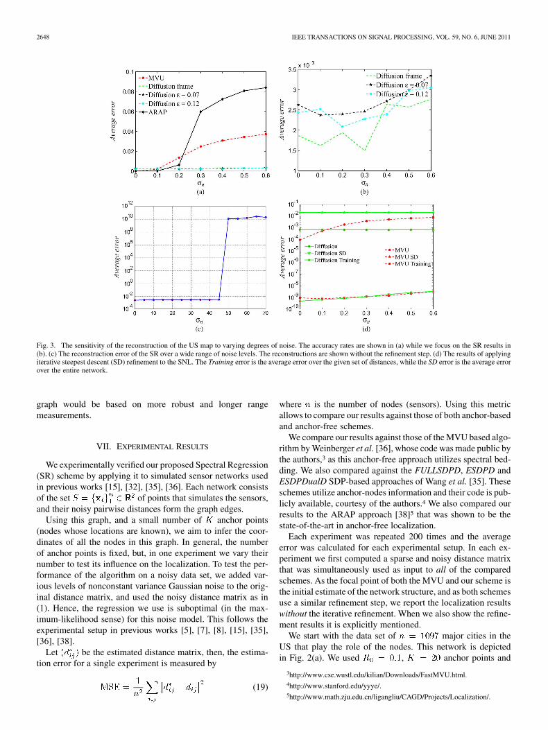
Fig. 3. The sensitivity of the reconstruction of the US map to varying degrees of noise. The accuracy rates are shown in (a) while we focus on the SR results in(b). (c) The reconstruction error of the SR over a wide range of noise levels. The reconstructions are shown without the refinement step. (d) The results of applyingiterative steepest descent (SD) refinement to the SNL. The Training error is the average error over the given set of distances, while the SD error is the average errorover the entire network.

graph would be based on more robust and longer rangemeasurements.

VII. EXPERIMENTAL RESULTS

We experimentally verified our proposed Spectral Regression(SR) scheme by applying it to simulated sensor networks usedin previous works [15], [32], [35], [36]. Each network consistsof the set of points that simulates the sensors,and their noisy pairwise distances form the graph edges.

Using this graph, and a small number of anchor points(nodes whose locations are known), we aim to infer the coor-dinates of all the nodes in this graph. In general, the numberof anchor points is fixed, but, in one experiment we vary theirnumber to test its influence on the localization. To test the per-formance of the algorithm on a noisy data set, we added var-ious levels of nonconstant variance Gaussian noise to the orig-inal distance matrix, and used the noisy distance matrix as in(1). Hence, the regression we use is suboptimal (in the max-imum-likelihood sense) for this noise model. This follows theexperimental setup in previous works [5], [7], [8], [15], [35],[36], [38].

Let be the estimated distance matrix, then, the estima-tion error for a single experiment is measured by

(19)

where is the number of nodes (sensors). Using this metricallows to compare our results against those of both anchor-basedand anchor-free schemes.

We compare our results against those of the MVU based algo-rithm by Weinberger et al. [36], whose code was made public bythe authors,3 as this anchor-free approach utilizes spectral bed-ding. We also compared against the FULLSDPD, ESDPD andESDPDualD SDP-based approaches of Wang et al. [35]. Theseschemes utilize anchor-nodes information and their code is pub-licly available, courtesy of the authors.4 We also compared ourresults to the ARAP approach [38]5 that was shown to be thestate-of-the-art in anchor-free localization.

Each experiment was repeated 200 times and the averageerror was calculated for each experimental setup. In each ex-periment we first computed a sparse and noisy distance matrixthat was simultaneously used as input to all of the comparedschemes. As the focal point of both the MVU and our scheme isthe initial estimate of the network structure, and as both schemesuse a similar refinement step, we report the localization resultswithout the iterative refinement. When we also show the refine-ment results it is explicitly mentioned.

We start with the data set of major cities in theUS that play the role of the nodes. This network is depictedin Fig. 2(a). We used , anchor points and

3http://www.cse.wustl.edu/kilian/Downloads/FastMVU.html.4http://www.stanford.edu/yyye/.5http://www.math.zju.edu.cn/ligangliu/CAGD/Projects/Localization/.


Fig. 4. The sensitivity of the reconstruction of the US cities map to different input parameters: (a) the maximal number of neighbors for each node within a radiusof � � �� and � � ��. (b) We repeat the analysis in (a) for the SR only and � � �� .(c) The number of embedding eigenvectors. We also testedthe stability to the number of anchor points in (d). In (e) and (f) we applied the different schemes with � � ��, and average node rank of 39 and 18,respectively. (a) � � ��, � � ��; (b) � � ��; (c) � � ��, � � ��; (d) � � ��; (e) � � ��; (f) � � ��.

neighbors at most that resulted in 57 k non zeroknown distances (out of an 0.5 M edges). We were unable torun the SDP based algorithms due to memory constraints. Weapplied the MVU scheme using ten eigenvectors, as this wasfound to be optimal by Weinberger et al. [36]. For the proposedSR scheme we used eigenvectors in all of our simulations(other than those in which we explicitly vary their number), and

bandwidths for the Diffusionframe.

The reconstructed networks are depicted in Figs. 2(b)–(h) andthe corresponding reconstruction error is shown in Fig. 3(a). Forlow noise levels the MVU and ARAP outperformed the SR pro-viding a close to perfect reconstruction, even without the itera-tive refinement step. As the noise increases, the accuracy of theMVU reconstruction decreases rapidly for and theARAP at . In contrast, the reconstruction accuracy ofthe SR degrades gradually and provides reasonable results for

[see Fig. 2(h)].The reconstruction error computed according to (19) is shown

in Fig. 3. It follows that for low noise values ofthe MVU and ARAP outperform the proposed scheme, but theproposed SR scheme was superior for . The benefitsof using the diffusion frame are depicted in Fig. 3(b), where formost noise values the Diffusion Frame is better than the singlebandwidth schemes.

In Section VI we discussed the spectral properties of theGraph Laplacian and related the noise effect to Wigner’sSemicircle Law. There we predicted that the proposed schemewill be robust to the noise, up to a certain amplitude of noise

at beyond which it will completely fail due to the cross over ofthe eigenvalues. This is evident in Fig. 3(c).

Recalling that the proposed scheme and the MVU aims at re-covering an initial estimate of the solution, to be used with aniterative refinement scheme (Section V-A), we tested the overallperformance of the localization schemes using the iterative re-finement procedure and the USA maps network. The results arereported in Fig. 3(d), where we first show the Training error.This is the average localization error of the refinement scheme,over the given set of distances. This error is directly minimizedby the iterative refinement scheme, and it follows that for bothschemes, it was on average of . As expected, the refine-ment schemes of both the SR and MVU converged to the sameerror due to the convexity of the localization problem given aninitial estimate.

We further studied the sensitivity of the proposed SR schemeto its different input parameters. First we consider , themaximal number of edges per node these are depicted inFigs. 4(a) and 4(b), while the number of eigenvectors used forthe adaptive spectral basis is tested in Fig. 4(c). The sensitivityof the reconstruction to the number of anchor points isstudied in Fig. 4(d). The sensitivity with respect to the sensingradius is studied in Figs. 4(e), 4(f), wherethe average node rank is 39 and 18, respectively. In thesefigures, we also compared our scheme and the MVU againstthe ARAP [38]. It follows that for low noise levelsthe ARAP outperforms both the MVU and SR. Yet, it shouldbenoted that both the MVU and SR results are shown withoutthe iterative refinement step, while the equivalent of the refine-


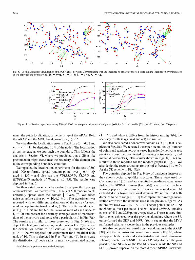
Fig. 5. Localization error visualization of the USA cities network. Corresponding true and localized nodes are connected. Note that the localization error increasesas we approach the boundary. (a) � � ��, � � �; (b) � � ��, � � ��.

Fig. 6. Localization experiment using 500 and 1000 random points drawn randomly over �� and used in [35]. (a) 500 points; (b) 1000 points.

ment, the patch localization, is the first step of the ARAP. Boththe ARAP and the MVU breakdown for

We visualize the localization error in Fig. 5 for and, by depicting 10% of the nodes. The localization

errors increase as we approach the boundary. This follows theanalysis in Section VI, where we predicted that a Gibbs-likephenomenon might occur near the boundary of the domain dueto the corresponding boundary condition.

We repeated the localization experiments for the sets of 500and 1000 uniformly spread random points overused in [35],6 and also ran the FULLSDPD, ESDPD andESDPDualD methods of Wang et al. [35]. The results xaredepicted in Fig. 6.

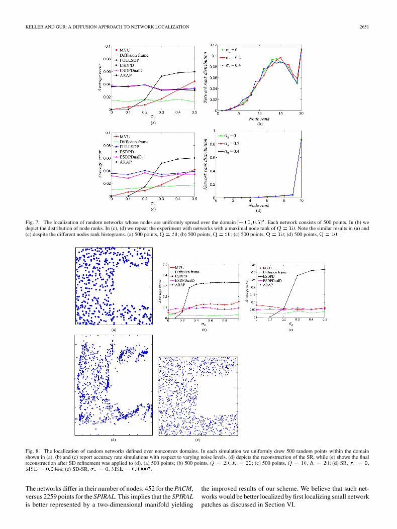
We then tested our scheme by randomly varying the topologyof the network. For that we drew 100 sets of 500 random pointsuniformly spread over the domain . We addednoise as before using . The experiment wasrepeated with ten different realizations of the noise (for eachrandom topology/network and ). The results are depictedin Fig. 7. First we limited the maximal rank of each node to

and present the accuracy averaged over of manifesta-tions of the network and noise (for a particular ) in Fig. 7(a).The results are similar to those presented in Fig. 6. We alsodepict the histogram of average node rank in Fig. 7(b), wherethe distribution seems to be Gaussian-like, and thresholdedat . We repeated this experiment for a maximal noderank of 10. This is depicted in Figs. 7(c) and (d). In this casethe distribution of node ranks is mostly concentrated around

6Available at: http://www.stanford.edu/~yyye/.

, and while it differs from the histogram Fig. 7(b), theaccuracy results (Figs. 7(a) and (c)) are similar.

We also considered a nonconvex domain as in [32] that is de-pictedin Fig. 8(a). We repeated the experimental set-up (numberof points and random networks) used in randomly networks testpreviously described, and tested for varying noise levels andmaximal noderanks . The results shown in Figs. 8(b), (c) aresimilar to those reported for the random graphs in Fig. 7. Wealso depict the reconstructions for the noise-freecasefor the SR scheme in Fig. 8(d).

The domains depicted in Fig. 9 are of particular interest asthey show special graph-like structures. These were used byCucuringu et al. [15], and are essentially one-dimensional man-ifolds. The SPIRAL domain (Fig. 9(b)) was used in machinelearning papers as an example of a one-dimensional manifoldembedded in a two-dimensional domain. We normalized bothdomains to be of range [ 1, 1] to compare their average local-ization error with the domains used in the previous figures. Asbefore, we used , anchor points andneighbors at most per node. The PACM and SPIRAL domainsconsist of 452 and 2259 points, respectively. The results are sim-ilar to ones achieved over the previous domains, where the SRoutperformed the SDP and MVU. Yet, it seems that the MVUperformed relatively worse than in the previous examples.

We also compared our results on these domains to the ARAP[38], and the reconstruction results are shown in Fig. 10, wherewe applied both the SR and a steepest-descent based refinementscheme, denoted as SD-SR. The ARAP outperformed the pro-posed SR and SD-SR on the PACM network, while the SR andSD-SR proved superior on the more difficult SPIRAL network.


Fig. 7. The localization of random networks whose nodes are uniformly spread over the domain �� . Each network consists of 500 points. In (b) wedepict the distribution of node ranks. In (c), (d) we repeat the experiment with networks with a maximal node rank of � � ��. Note the similar results in (a) and(c) despite the different nodes rank histograms. (a) 500 points, � � ��; (b) 500 points, � � ��; (c) 500 points, � � ��; (d) 500 points, � � ��.

Fig. 8. The localization of random networks defined over nonconvex domains. In each simulation we uniformly drew 500 random points within the domainshown in (a). (b) and (c) report accuracy rate simulations with respect to varying noise levels. (d) depicts the reconstruction of the SR, while (e) shows the finalreconstruction after SD refinement was applied to (d). (a) 500 points; (b) 500 points, � � ��, � � ��; (c) 500 points, � � ��, � � ��; (d) SR, � � �,� � ��; (e) SD-SR, � � �, � � �� .

The networks differ in their number of nodes: 452 for the PACM,versus 2259 points for the SPIRAL. This implies that the SPIRALis better represented by a two-dimensional manifold yielding

the improved results of our scheme. We believe that such net-works would be better localized by first localizing small networkpatches as discussed in Section VI.


Fig. 9. Localization of the domains with special topology used by Cucuringu et. al. [15]. The localization results of the PACM (a) and SPIRAL (b) networks aredepicted in Figs. (c) and (d), respectively. (a); (b) 500 points; (c) PACM; (d) SPIRAL.

Fig. 10. Localization results for PACM and SPIRAL domains. For the PACM we normalized the largest dimension to [0,1] and set � � �� and � � �. Forthe SPIRAL we set � � �� and � � �. (a) SR, � � �, �� ; (b) SR, �� ; (c) SD-SR, � � �, �� ; (d) SD-SR,�� ; (e) ARAP, � � �, �� ; (f) ARAP, �� .

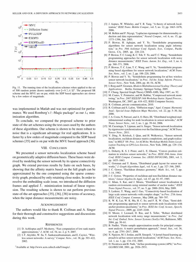
One of the upsides of the proposed scheme is its relativelylow computational time and complexity. The running time ofthe compared algorithms are depicted in Fig. 11, and it follows

that the SDP based schemes are slower by a few orders of mag-nitude, and the same applies to the ARAP. We run the timingsimulations on a 2.8 GHz Intel Quad computer. Our SR scheme


Fig. 11. The running time of the localization schemes when applied to the setof 500 random points drawn randomly over �� . The proposed SRscheme and the MVU are on par, while the SDP based approaches are slowerby a few orders of magnitude.

was implemented in Matlab and was not optimized for perfor-mance. We used Romberg’s -Magic package7 as our min-imization algorithm.

To conclude, we compared the proposed scheme to priorstate-of-the-art schemes using the test cases used by the authorsof these algorithms. Our scheme is shown to be more robust tonoise that is a significant advantage for real applications. It isfaster by a few orders of magnitude compared to the SDP basedschemes [35] and is on par with the MVU based approach [36].

VIII. CONCLUSION

We presented a sensor networks localization scheme basedon geometrically adaptive diffusion bases. These bases were de-rived by modeling the sensor network by its sparse connectivitygraph. We extend previous results by Saito on such bases, byshowing that the affinity matrix based on the full graph can beapproximated by the one computed using the sparse connec-tivity graph, produced by only retaining close nodes. In order toresolve the embedding scale issue, we introduced the diffusionframes and applied minimization instead of linear regres-sion. The resulting scheme is shown to out perform previousstate-of-the-art approaches [35], [36], [38] in terms of accuracy,when the input distance measurements are noisy.

ACKNOWLEDGMENT

The authors would like to thank R. Coifman and A. Singerfor their thorough and constructive suggestions and discussionsduring this work.

REFERENCES

[1] D. Achlioptas and F. Mcsherry, “Fast computation of low-rank matrixapproximations,” J. ACM, vol. 54, no. 2, p. 9, 2007.

[2] I. F. Akyildiz, W. Su, Y. Sankarasubramaniam, and E. Cayirci, “Wire-less sensor networks: A survey,” Comput. Netw., vol. 38, pp. 393–422,2002.

7Available at: http://www.acm.caltech.edu/l1magic/.

[3] J. Aspnes, W. Whiteley, and Y. R. Yang, “A theory of network local-ization,” IEEE Trans. Mobile Comput., vol. 5, no. 12, pp. 1663–1678,2006.

[4] M. Belkin and P. Niyogi, “Laplacian eigenmaps for dimensionality re-duction and data representation,” Neural Comput., vol. 6, no. 15, pp.1373–1396, Jun. 2003.

[5] P. Biswas, H. Aghajan, and Y. Ye, “Semidefinite programmingalgorithms for sensor network localization using angle informa-tion,” in Pro. 39th Asilomar Conf. Signals, Syst., Comput., PacificGrove, CA, 2005, pp. 220–224.

[6] P. Biswas, T. C. Liang, K. C. Toh, Y. Ye, and T. C. Wang, “Semidefiniteprogramming approaches for sensor network localization with noisydistance measurements,” IEEE Trans. Autom. Sci. Eng., vol. 3, no. 4,pp. 360–371, 2006.

[7] P. Biswas, T. C. Lian, T. C. Wang, and Y. Ye, “Semidefinite program-ming based algorithms for sensor network localization,” ACM Trans.Sen. Netw., vol. 2, no. 2, pp. 188–220, 2006.

[8] P. Biswas and Y. Ye, “Semidefinite programming for ad hoc wirelesssensor network localization,” in Proc. 3rd Int. Symp. Inform. Process.Sensor Netw., New York, 2004, pp. 46–54, ACM.

[9] I. Borg and P. Groenen, Modern Multidimensional Scaling: Theory andApplications. Berlin, Germany: Springer-Verlag, 2005.

[10] F. Chung, Spectral Graph Theory CBMS-AMS, May 1997, no. 92.[11] M. Coates, Y. Pointurier, and M. Rabbat, “Compressed network moni-

toring,” in Proc. 2007 IEEE/SP 14th Workshop Statist. Signal Process.,Washington, DC, 2007, pp. 418–422, IEEE Computer Society.

[12] R. Coifman, private communication, 2010.[13] R. Coifman and S. Lafon, “Diffusion maps,” Appl. Comput. Harmonic

Anal.: Special Issue Diffusion Maps Wavelets, vol. 22, pp. 5–30, Jul.2006.

[14] J. A. Costa, N. Patwari, and A. O. Hero, III, “Distributed weighted-mul-tidimensional scaling for node localization in sensor networks,” ACMTrans. Sensor Netw., vol. 2, no. 1, pp. 39–64, 2006.

[15] M. Cucuringu, Y. Lipman, and A. Singer, “Sensor network localizationby eigenvector synchronization over the Euclidean group,” ACM Trans.Sensor Netw., 2011.

[16] Y. Ding, N. Krislock, J. Qian, and H. Wolkowicz, “Sensor networklocalization, euclidean distance matrix completions, and graph realiza-tion,” in MELT ’08: Proc. 1st ACM Int. Workshop Mobile Entity Local-ization Tracking in GPS-Less Environ., New York, 2008, pp. 129–134,ACM.

[17] L. Doherty, K. S. J. Pister, and L. E. Ghaoui, “Convex position esti-mation in wireless sensor networks,” in Proc. IEEE 20th Annu. JointConf. IEEE Comput. Commun. Soc. (IEEE INFOCOM), 2001, vol. 3,pp. 1655–1663.

[18] C. Gotsman and Y. Koren, “Distributed graph layout for sensor net-works,” J. Graph Algorithms Appl., vol. 9, no. 3, pp. 327–346, 2005.

[19] J. C. Gower, “Euclidean distance geometry,” Math. Sci., vol. 7, pp.1–14, 1982.

[20] J. C. Gower, “Properties of euclidean and non-Euclidean distance ma-trices,” Linear Algebra Its Appl,, vol. 67, pp. 81–97, 1985.

[21] U. Khan, S. Kar, and J. Moura, “Distributed sensor localization inrandom environments using minimal number of anchor nodes,” IEEETrans Signal Process., vol. 57, no. 5, pp. 2000–2016, May 2009.

[22] S. Lederer, Y. Wang, and J. Gao, “Connectivity-based localization oflarge scale sensor networks with complex shape,” in Proc. 27th Annu.IEEE Conf. Comput. Commun., May 2008, pp. 789–797.

[23] K. W. K. Lui, W. K. Ma, H. C. So, and F. K. W. Chan, “Semi-defi-nite programming approach to sensor network node localization withanchor position uncertainty,” in Proc. IEEE Int. Conf. Acoust., Speech,Signal Process., 2009, pp. 2245–2248.

[24] D. Moore, J. Leonard, D. Rus, and S. Teller, “Robust distributednetwork localization with noisy range measurements,” in Proc. 2ndInt. Conf. Embed. Netw. Sensor Systems (SenSys’04), Baltimore, MD,2004, pp. 50–61.

[25] B. Nadler, “Finite sample approximation results for principal compo-nent analysis: A matrix perturbation approach,” Annal. Stat., vol. 36,no. 6, pp. 2791–2817, 2008.

[26] X. Nguyen, M. I. Jordan, and B. Sinopoli, “A kernel-based learning ap-proach to ad hoc sensor network localization,” ACM Trans. Sen. Netw.,vol. 1, no. 1, pp. 134–152, 2005.

[27] D. Niculescu and B. Nath, “Ad hoc positioning system (APS),” in Proc.GLOBECOM, 2001, pp. 2926–2931.


[28] N. Patwari, J. N. Ash, S. Kyperountas, A. O. Hero, R. L. Moses, andN. S. Correal, “Locating the nodes: Cooperative localization in wire-less sensor networks,” IEEE Signal Process. Mag. vol. 22, no. 4, pp.54–69, 2005 [Online]. Available: http://dx.doi.org/10.1109/MSP.2005.1458287

[29] N. Patwari, I. Hero, A. O. , M. Perkins, N. Correal, and R. O’Dea, “Rel-ative location estimation in wireless sensor networks,” IEEE Trans.Signal Process., vol. 51, no. 8, pp. 2137–2148, Aug. 2003.

[30] N. Saito, “Data analysis and representation on a general domain usingeigenfunctions of Laplacian,” Appl. Comput. Harmonic Anal., vol. 25,pp. 68–97, 2007.

[31] C. Savarese, J. M. Rabaey, and K. Langendoen, “Robust positioningalgorithms for distributed ad-hoc wireless sensor networks,” in Proc.General Track Annu. Conf. USENIX Annu. Techn. Conf., Berkeley, CA,2002, pp. 317–327, USENIX Association.

[32] Y. Shang, W. Ruml, Y. Zhang, and M. Fromherz, “Localization fromconnectivity in sensor networks,” IEEE Trans. Parallel Distrib. Syst.,vol. 15, no. 11, pp. 961–974, 2004.

[33] J. P. Sheu, P. C. Chen, and C. S. Hsu, “A distributed localizationscheme for wireless sensor networks with improved grid-scan andvector-based refinement,” IEEE Trans. Mobile Comput., vol. 7, no. 9,pp. 1110–1123, 2008.

[34] A. Singer, “A remark on global positioning from local distances,” Proc.Nat. Acad. Sci., vol. 105, no. 28, pp. 9507–9511, 2008.

[35] Z. Wang, S. Zheng, Y. Ye, and S. Boyd, “Further relaxations of thesemidefinite programming approach to sensor network localization,”SIAM J. Optimization, vol. 19, no. 2, pp. 655–673, 2008.

[36] K. Q. Weinberger, F. Sha, Q. Zhu, and L. K. Saul, “Graph laplacian reg-ularization for large-scale semidefinite programming,” in Proc. NIPS,2006, pp. 1489–1496.

[37] J. G. Yue Wang and S. Lederer, “Connectivity-based sensor networklocalization with incremental Delaunay refinement method,” in Proc.28th Annu. IEEE Conf. Comput. Commun., 2009.

[38] L. Zhang, L. Liu, C. Gotsman, and S. J. Gortler, “An as-rigid-as-pos-sible approach to sensor network localization,” ACM Trans. SensorNetw., 2010.

Yosi Keller received the B.Sc. degree in electricalengineering from the Technion-Israel Institute ofTechnology, Haifa, Israel, in 1994. He received theM.Sc. and Ph.D. degrees in electrical engineeringfrom Tel-Aviv University, Tel-Aviv, in 1998 and2003, respectively.

From 1994 to 1998, he was a R&D Officer in theIsraeli Intelligence Force. From 2003 to 2006, hewas a Gibbs Assistant Professor with the Departmentof Mathematics, Yale University. He is currently aSenior Lecturer at the Electrical Engineering Depart-

ment in Bar Ilan University, Israel. His research interests include graph baseddata analysis, optimization, and spectral graph theory-based dimensionalityreduction.

Yaniv Gur received the BS.c. and M.A. degrees inphysics from the Technion-Israel Institute of Tech-nology, Haifa, Israel, in 1999 and 2004, respectively.He received the Ph.D. degree in applied mathematicsfrom Tel-Aviv University, Tel-Aviv, Israel, in 2008.

From 2008 to 2010, he was a Postdoctoral Re-search Associate at the School of Engineering in BarIlan University, and a Researcher at the TechnionResearch and Development Foundation in Haifa.Since October 2010, he is a Postdoctoral ResearchAssociate at SCI Institute, University of Utah, Salt

Lake City. His research interests include variational and PDE methods in imageprocessing, shape analysis, optimization, and assignment problems.

keller 2011

Documents