kinematic analysis of mechanisms. relative velocity and

Chapter 2Kinematic Analysis of Mechanisms.Relative Velocity and Acceleration.Instant Centers of Rotation

Abstract Kinematic analysis of a mechanism consists of calculating position,velocity and acceleration of any of its points or links. To carry out such an analysis,we have to know linkage dimensions as well as position, velocity and accelerationof as many points or links as degrees of freedom the linkage has. We will point outtwo different methods to calculate velocity of a point or link in a mechanism: therelative velocity method and the instant center of rotation method.

2.1 Velocity in Mechanisms

We will point out two different methods to calculate velocity of a point or link in amechanism: the relative velocity method and the instant center of rotation method.However, before getting into the explanation of these methods, we will introducethe basic concepts for their development.

2.1.1 Position, Displacement and Velocity of a Point

To analyze motion in a system, we have to define its position and displacementpreviously. The movement of a point is a series of displacements in time, alongsuccessive positions.

2.1.1.1 Position of a Point

The position of a point is defined according to a reference frame. The coordinatesystem in a plane can be Cartesian or polar (Fig. 2.1).

© Springer International Publishing Switzerland 2016A. Simón Mata et al., Fundamentals of Machine Theory and Mechanisms,Mechanisms and Machine Science 40, DOI 10.1007/978-3-319-31970-4_2

21

In any coordinate system, we have to define the following:

• Origin of coordinates: starting point from where measurements start.• Axis of coordinates: established directions to measure distances and angles.• Unit system: units to quantify distances.

If a polar coordinate system is used, the position of a point is defined by a vectorcalled rPO connecting the origin of coordinates O with the mentioned point. If O is apoint on the frame this vector gives us the absolute position of point P and we willcall it rP.

In most practical situations, an absolute reference system, considered stationary,is used. The stationary system coordinates do not depend on time. The absoluteposition of a point is defined as its position seen from this absolute referencesystem. If the reference system moves with respect to a stationary system, theposition of the point is considered a relative position.

Anyway, this choice is not fundamental in kinematics as the movements to bestudied will be relative. Take, for example, the suspension of a car where move-ments might refer to the car body, without considering whether the car is moving ornot. Movements in the suspension system can be regarded as absolute motion withrespect to the car body.

2.1.1.2 Displacement of a Point

When a point changes its position, a displacement takes place. If at instant t thepoint is at position P and at instant tþDt, the point is at P0, displacement during Dtis defined as the vector that measures the change in position (Eq. 2.1):

Dr ¼ rP0 � rP ð2:1Þ

Displacement is a vector that connects point P at instant t with point P0 at instanttþDt and does not depend on the path followed by the point but on the initial andfinal positions (Fig. 2.2).

Y

(a) (b)

XO

P

Px

Py

Y

XO

P

POr

Fig. 2.1 a Cartesian andpolar coordinates of point P ina plane. b Polar coordinates ofthe same point

22 2 Kinematic Analysis of Mechanisms. Relative Velocity …

2.1.1.3 Velocity of a Point

The ratio between point displacement and time spent carrying it out is referred to asaverage velocity of that point. Therefore, average velocity is a vector of magnitudeDr=Dt and has the same direction as displacement vector Dr. If the time duringwhich displacement takes place is close to zero, the velocity of the point is calledinstant velocity, or simply velocity (Eq. 2.2):

v ¼ limDt!0

DrDt

¼ drdt

ð2:2Þ

The instant velocity vector magnitude is dr=dt. In an infinitesimal positionchange, the direction of the displacement vector coincides with the trajectory. WhenO is the instantaneous center of the trajectory of point P, we can express the instantvelocity magnitude as Eq. (2.3):

vP ¼ drdt

¼ dsdt

¼ dhdt

� rP ¼ x � rP ð2:3Þ

The direction of this velocity is the same as dr which, at the same time, istangent to the motion trajectory of point P (Fig. 2.3).

2.1.2 Position, Displacement and Angular Velocityof a Rigid Body

Any movement of a rigid body can be considered a combination of two motions: thedisplacement of a point in the rigid body and its rotation with respect to the point.

Fig. 2.2 Displacement ofpoint P in a plane duringinstant Dt

Fig. 2.3 Displacement ofpoint P in a plane duringinstant dt close to zero

2.1 Velocity in Mechanisms 23

In the last section, we defined the displacement of a point, so the next subject tobe studied is the rotation of a rigid body.

2.1.2.1 Angular Position of a Rigid Body

To define the angular position of a rigid body, we just need to know the angleformed by the axis of the coordinate system and reference line AB (Fig. 2.4).

2.1.2.2 Angular Displacement of a Rigid Body

When a rigid body changes its angular position from hAB to hA0B0 , angular dis-placement DhAB takes place (Fig. 2.5).

hA0B0 ¼ hAB þDhAB ð2:4Þ

The angular displacement of a rigid body, DhAB, does not depend on the tra-jectory followed but on the initial and final angular position (Eq. 2.4).

2.1.2.3 Angular Velocity of a Rigid Body

We define the angular velocity of a rigid body as the ratio between angular dis-placement and its duration. If this time is, dt close to zero, this velocity is calledinstant angular velocity or simply angular velocity (Eq. 2.5).

Fig. 2.4 Angular position ofa rigid body hAB

Fig. 2.5 Angulardisplacement of a rigid bodyDhAB


xAB ¼ dhABdt

ð2:5Þ

2.1.3 Relative Velocity Method

In this section we will develop the relative velocity method that will allow calcu-lating linear and angular velocities of points and links in a mechanism.

2.1.3.1 Relative Velocity Between Two Points

Let A be a point that travels from position A to position A0 during time interval Dtand let B be a point that moves from position B to position B0 in the same timeinterval (Fig. 2.6).

Absolute displacements of points A and B are given by vectors DrA and DrB.Relative displacement of point B with respect to A is given by vector DrBA, so itverifies (Eq. 2.6):

DrB ¼ DrA þDrBA ð2:6Þ

In other words, we can consider that point B moves to position B0 with dis-placement equal to the one for point A to reach point B00 followed by anotherdisplacement, from point B00 to point B0. The latter coincides with vector DrBA forrelative displacement. We can assert the same for the displacement of pointA (Eq. 2.7), hence:

DrA ¼ DrB þDrAB ð2:7Þ

Evidently DrBA and DrAB are two vectors with the same magnitude but oppositedirections.

Fig. 2.6 Absolute displacements of points A and B, DrA and DrB, and relative displacement ofpoint B with respect to A, DrBA


If we regard these as infinitesimal displacements and relate them to time dt, thetime it took them to take place, we obtain the value of the relative velocities byEq. (2.8):

drBdt

¼ drAdt

þ drBAdt

) vB ¼ vA þ vBA ð2:8Þ

Therefore, the velocity of a point can be determined by the velocity of anotherpoint and their relative velocity.

As we have mentioned before, relative displacements DrBA and DrAB haveopposite directions. Therefore relative velocities vBA and vAB will be two vectorswith the same magnitude that also have opposite directions (Eq. 2.9).

vBA ¼ �vAB ð2:9Þ

2.1.3.2 Relative Velocity Between Two Points of the Same Link

Let AB be a reference line on a body that changes its position to A0B0 during timeinterval Dt.

As studied in the previous section, the vector equation for the displacement ofpoint B is Eq. (2.6) (Fig. 2.7a). In the case of A and B belonging to the same body,distance AB does not change, so the only possible relative movement between A andB is a rotation of radius AB. This way, relative displacement will always be arotation of point B about point A (Fig. 2.7b).

If we divide these displacements by the time interval in which they happened,we obtain Eq. (2.11):

DrBDt

¼ DrADt

þ DrBADt

) VB ¼ VA þVBA ð2:10Þ

(a) (b)

Fig. 2.7 a Relative displacement of point B with respect to point A (both being part of the samelink). b Rotation of point B about point A


The value of VBA (average relative velocity of point B with respect to point A)can be determined by using Eq. (2.11):

VBA ¼ DrBADt

¼ 2 sinðDh=2ÞDt

ð2:11Þ

where Dh is the angular displacement of body AB (Fig. 2.7b). If all displacementstake place during an infinitesimal period of time, dt, then average velocities becomeinstant velocities (Eq. 2.12):

vB ¼ vA þ vBA ð2:12Þ

This way, the velocity of point B can be obtained by adding relative instantvelocity vBA to the velocity of point A.

To obtain the magnitude of relative instant velocity vBA in Eq. (2.13), we have toconsider that the time during which displacement takes place is close to zero inEq. (2.11)

vBA ¼ limDt!0

DrBADt

¼ 2 sinðdh=2Þdt

AB ’ dhdt

AB ¼ xAB ð2:13Þ

Therefore, any point on a rigid body, such as B, moves relatively to any otherpoint on the same body, such as A, with velocity vBA, which can be expressed as avector of magnitude equal to the product of the angular velocity of the bodymultiplied by the distance between both points (Eq. 2.14). Its direction is given bythe angular velocity of the body, perpendicular to the straight line connecting bothpoints (Fig. 2.8).

vBA ¼ x ^ rBA ð2:14Þ

2.1.3.3 Application of the Relative Velocity Method to One Link

Equation (2.13) is the basis for the relative velocity method. It is a vector equationthat allows us to calculate two algebraic unknowns such as one magnitude and onedirection, two magnitudes or two directions.

Fig. 2.8 Relative velocity ofpoint B with respect to pointA (both being part of the samelink)


Figure 2.9a shows points A and B of a link moving at unknown angular velocityx. Suppose that we know the velocity of point A, vA, and the velocity direction ofpoint B. To calculate the velocity magnitude of point B, we use Eq. (2.13).Studying every parameter in the equation:

• vA is a vector defined as vA ¼ vAx iþ vAy j with known magnitude and direction.• vB is a vector with known direction and unknown magnitude. Assuming it is

moving upward to the left (Fig. 2.9a), the direction of this vector will be givenby angle θ and it will be defined as Eq. (2.15):

vB ¼ vB cos hiþ vB sin hj ð2:15Þ

• vBA is a vector of unknown magnitude due to the fact that we do not know theangular velocity value, ω, of the rigid body. Its direction is perpendicular tosegment line AB (Fig. 2.9b). Therefore, it can be obtained in Eq. (2.16):

vBA ¼ x ^ rBA ¼i j k

0 0 x

rBAx rBAy 0

�� ¼

i j k

0 0 x

BA cos hBA BA sin hBA 0

��

¼ �rBAyxiþ rBAxxj ¼ BAxð� sin hBA iþ cos hBAjÞ

ð2:16Þ

where rBAx ¼ AB cos hAB and rBAy ¼ AB sin hAB.

If we plug the velocity vectors into Eq. (2.13), we obtain Eq. (2.17):

vB cos hiþ vB sin hj ¼ vAx iþ vAy j� rBAxxiþ rBAyxj

¼ vAx iþ vAy j� BAx sin hBAiþBAx cos hBA jð2:17Þ

If we break the velocity vectors in the equation into their components, twoalgebraic equations are obtained (Eq. 2.18):

(a) (b)

Fig. 2.9 a Calculation of the point B velocity magnitude knowing its direction and vector vA.b Velocity diagram


vB cos h ¼ vAx � BAx sin hBAvB sin h ¼ vAy þBAx cos hBA

�ð2:18Þ

We get two equations where the vB magnitude and angular velocity ω are theunknowns, so the problem is completely defined. Once the magnitudes have beencalculated by solving the system of Eq. (2.18), we obtain the rotation direction of ωand the direction of vB depending on the + or − magnitude sign. In the example inFig. 2.9a, the values obtained from Eq. (2.18) are positive for angular velocity ω aswell as for the velocity magnitude of point B, vB. This means that both have samedirections from the ones that were assumed to write the equations. Therefore, pointB moves upward right and the body rotates counterclockwise.

Equation (2.13) can also be solved graphically using a velocity diagram(Fig. 2.9b). Starting from point o (velocity pole), a straight line equal to the value ofknown velocity vA is drawn using a scale factor. The velocity polygon is closeddrawing the known direction of vB from the pole and velocity direction vBA (per-pendicular to AB) from the end point of vA. The intersection of these two directionsdefines the end points of vectors vBA and vB. Measuring their length and using thescale factor, we obtain their magnitudes.

2.1.3.4 Calculation of Velocities in a Four-Bar Mechanism

Figure 2.10 represents a four-bar linkage in which we know the dimensions of allthe links: O2A, AB, O4B and O2O4. This mechanism has one degree of freedom,which means that the position and velocity of any point on any link can bedetermined from the position and velocity of one link. Assume that we know h2 andx2 and that we want to find the values of h3, h4, x3 and x4. To calculate h3 and h4,we can simply draw a scale diagram of the linkage at position h2 (Fig. 2.10) orsolve the necessary trigonometric equations (Appendix A).

Once the link positions are obtained, we can start determining the velocities.First, velocity vA will be calculated:

Fig. 2.10 Four-bar linkagewhere all the link dimensionsare know as well as theposition and velocity of link 2


• The horizontal and vertical components of vA are given by the expression(Eq. 2.19):

vA ¼ x2 ^ rAO2 ¼i j k0 0 x2

AO2 cos h2 AO2 sin h2 0

�� ð2:19Þ

As the direction of x2 is counterclockwise (Fig. 2.10), its value in the previousequation will be negative. Point A describes a rotational motion about O2 with aradius of r2 ¼ O2A and an angular velocity of x2, so the direction of vA will beperpendicular to O2A to the left according to the rotation of link 2 (Fig. 2.11).

• Once vA is known, we can obtain vB with the following expression (Eq. 2.20):

vB ¼ x4 ^ rBO4 ¼i j k0 0 x4

BO4 cos h4 BO4 sin h4 0

�� ð2:20Þ

Since point B rotates about steady point O4 with a radius of BO4 and an angularvelocity of x4, we cannot calculate the magnitude of vB due to the fact that x4 isunknown. The direction of the linear velocity of point B has to be perpendicularto turning radius BO4 (Eq. 2.21). We can use the relative velocity method to findthe magnitude of velocity vB:


Vector vA as well as the direction of vector vB are known in vector equa-tion (2.21). We will now study vector vBA.

• The horizontal and vertical components of the point B relative velocity con-sidering its rotation about point A are (Eq. 2.22):

vBA ¼ x3 ^ rBA ¼i j k0 0 x3

BA cos h3 BA sin h3 0

�� ð2:22Þ

Fig. 2.11 Velocity diagramfor the given position andvelocity of link 2


Since the angular velocity of link 3 is unknown, we cannot calculate the mag-nitude of vBA. The direction of vBA is known since the relative velocity of a pointthat rotates about another is always perpendicular to the radius joining them. In thiscase, the direction will be perpendicular to BA.

This way we confirm that Eq. (2.21) has two unknowns. In (Fig. 2.11) thisequation is solved graphically to calculate the vBA and vB magnitudes the same wayas in Fig. 2.9.

If we want to solve Eq. (2.21) mathematically, the unknowns are the x3 and x4

magnitudes. To obtain these values, we have to solve the vector equation(Eq. 2.23):

i j k

0 0 x4


�� ¼

i j k

0 0 x2


��

þi j k

0 0 x3


��

ð2:23Þ

By developing and separating components, we obtain two algebraic equations(Eq. 2.24) where we can clear x3 and x4.

BO4x4 sin h4 ¼ AO2x2 sin h2 þBAx3 sin h3BO4x4 cos h4 ¼ AO2x2 cos h2 þBAx3 cos h3

�ð2:24Þ

Once the angular velocities are obtained, we can represent velocities vA, vB andvBA according to their components (Fig. 2.11).

Assume that we add point C to link 3 in the previous mechanism as shown inFig. 2.12a and that we want to calculate its velocity. In this case, the value of angleh03 is already known since angle β is a given value of the problem. Hence,h03 ¼ 360� � ðb� h3Þ.

To obtain the velocity of point C once x3 has been determined, we make use ofvector equation vC ¼ vA þ vCA, vCA where is perpendicular to CA and its value is:

(a) (b)

Fig. 2.12 a Four-bar linkage with new point C on link 3. b Velocity diagram


vCA ¼ x3 ^ rCA ¼i j k0 0 x3

CA cos h03 CA sin h03 0

�� ð2:25Þ

Vector vCA is obtained directly from Eq. (2.25) since angular velocity x3 isalready known. vC can be calculated adding the two known vectors, vA and vCA.The velocity of point C can also be calculated based on the velocity of point B byusing Eq. (2.26)

vC ¼ vB þ vCB ð2:26Þ

Figure 2.12b shows the calculation of vC graphically.

2.1.3.5 Velocity Calculation in a Crankshaft Linkage

To calculate link velocities in a crankshaft linkage such as the one in Fig. 2.13, westart by calculating the positions of links 3 and 4. We consider that dimensions O2Aand AB are already known as well as the direction of the piston trajectory line andits distance rBy to O2. If we draw a scale diagram of the linkage, the positions oflinks 3 and 4 are determined for a given position of link 2. We can also obtain theirposition by solving the following trigonometric equations (Eq. 2.27) (Appendix A):

l ¼ arcsinO2A sin h2 þ rBy

ABrBx ¼ O2A cos h2 þAB cos lh3 ¼ 360� � l

9>=>; ð2:27Þ

From this point, the calculation of the velocity of point A is the same as the onepreviously done for the four-bar linkage (Eq. 2.28).

vA ¼ x2 ^ r2 ¼i j k0 0 x2

r2 cos h2 r2 sin h2 0

�� ð2:28Þ

Fig. 2.13 Crankshaftlinkage: positions of links 3and 4 are determined for agiven position of link 2


Since point A is rotating with respect to steady point O2, the direction of velocityvA is perpendicular to O2A and it points in the same direction as the angular velocityof link 2, that is, x2.

We will now study velocity vB:

• The magnitude of velocity vB is unknown. As the trajectory of point B movesalong a straight line, its turning radius is infinite and its angular velocity is zero.Therefore, we cannot determine its velocity magnitude in terms of its angularvelocity and turning radius.

• The direction of vB is the same as the trajectory of the piston, XX 0.Consequently, velocity vB can be written as Eq. (2.29):

vB ¼ vBi ð2:29Þ

To calculate vB we need to make use of the relative velocity method (Eq. 2.30):


The magnitude and direction of vector vBA are given by Eq. (2.31):



�� ð2:31Þ

Plugging the results into velocity equation (2.30), we obtain Eq. (2.32):

vBi ¼i j k0 0 x2


��þ

i j k0 0 x3


�� ð2:32Þ

Breaking it into its components, we define the following equation system(Eq. 2.33):

vB ¼ �AO2x2 sin h2 � BAx3 sin h30 ¼ AO2x2 cos h2 þBAx3 cos h3

�ð2:33Þ

From which the magnitude of velocity vB and angular velocity x3 are obtained.Once these velocities are known, we can represent them as shown in Fig. 2.14.

2.1.3.6 Velocity Analysis in a Slider Linkage

To analyze the slider linkage in Fig. 2.15a, we will start by calculating the positionof links 3 and 4. As in previous examples, we know the length and position of link


2 as well as the distance between both steady supports O2O4. The position of link 4is graphically determined by the line that joins O4 and A. If we use trigonometry forour analysis, the equations needed are (Eq. 2.34) (Appendix A):

O4A ¼ffiffiffiffiffiffiffiffiffiffiffiffiffiffiffiffiffiffiffiffiffiffiffiffiffiffiffiffiffiffiffiffiffiffiffiffiffiffiffiffiffiffiffiffiffiffiffiffiffiffiffiffiffiffiffiffiffiffiffiffiffiffiffiffiffiffiffiffiffiffiffiffiffiffiffiffiffiffiffiffiffiffiffiffiffiffiffiffiffiO2O4

2 þO2A2 � 2 O2O4 O2A cosð270� � h2Þ

qh4 ¼ arccos O2A cos h2

O4A

9=; ð2:34Þ

In the diagram, let A be a point that belongs to links 2 and 3 as in previousexamples for the four-bar and crank-shaft linkages. It is not necessary to distinguishA2 and A3 as they are actually the same point. However, there is another point, A4 inlink 4, which coincides with A2 at the instant represented in Fig. 2.15a.Nonetheless, point A4 rotates about steady point O4 while A2 rotates about O2. Dueto this, they follow different trajectories at different velocities.

The velocity of point A2 is perpendicular to O2A and its magnitude and directionare represented by Eq. (2.35):

vA2 ¼ x2 ^ r2 ¼i j k0 0 x2

r2 cos h2 r2 sin h2 0

�� ð2:35Þ

The velocity of A4 is perpendicular to O4A and its magnitude is unknownbecause it depends on the angular velocity of link 4. Since point A4 belongs to link4 and it is rotating about steady point O4, its velocity is represented by Eq. (2.36):

Fig. 2.14 Calculation ofvelocities in a crankshaftlinkage

(a) (b)Fig. 2.15 Slider linkage:a positions of links 3 and 4are determined for a givenposition of link 2,b calculation of velocities in aslider linkage


vA4 ¼ x4 ^ rA4O4 ¼i j k0 0 x4

A4O4 cos h4 A4O4 sin h4 0

�� ð2:36Þ

To calculate vA4 , we will make use of the relative velocity method (Eq. 2.37):

vA2 ¼ vA4 þ vA2A4 ð2:37Þ

To calculate the velocities and solve this vector equation, we have to studyvector vA2A4 first:

• The magnitude of vA2A4 is unknown and represents the velocity at which link 3slides over link 4.

• The direction of vA2A4 coincides with direction O4A. Therefore, this velocity isrepresented by Eq. (2.38):

vA2A4 ¼ vA2A4 cos h4iþ vA2A4 sin h4 j ð2:38Þ

Using Eq. (2.37), we obtain Eq. (2.39) with two algebraic unknowns (angularvelocity x4 and the magnitude of velocity vA2A4 ):

i j k

0 0 x2


�� ¼

i j k

0 0 x4

O4A cos h4 O4A sin h4 0

��

þ vA2A4 cos h4iþ vA2A4 sin h4 j

ð2:39Þ

This can be solved by breaking the equation into its components (Eq. 2.40):

�AO2x2 sin h2 ¼ �O4Ax4 sin h4 þ vA2A4 cos h4

AO2x2 cos h2 ¼ O4Ax4 cos h4 þ vA2A4 sin h4

)ð2:40Þ

Once the velocities have been obtained, we can represent them in the polygonshown on Fig. 2.15b.

2.1.3.7 Velocity Images

In the velocity polygon shown in Fig. 2.16b, the sides of triangle Mabc are per-pendicular to those of triangle MABC of the linkage in Fig. 2.16a. The reason forthis is that relative velocities are always perpendicular to their radius and, conse-quently, triangles Mabc and MABC are similar, with a scale ratio that depends onx3. The velocity image of link 3 is a triangle similar to the link, rotated 90° in thedirection of x3.


Every side or link has its image in the velocity polygon. This way ab, bc and acare the images of AB, BC and AC respectively. Vector oa�! ¼ vA starting at pole o is

the image of O2A and vector ob�! ¼ vB is the image of O4B. Moreover, the image of

the frame link is pole o with null velocity. We can verify that velocities departingfrom o are always absolute velocities while velocities departing from any otherpoint are relative ones.

If we add point M to link 3 of the linkage in Fig. 2.16a, we can obtain itsvelocity in the velocity polygon by looking for its image. We can verify thatdistance am in the velocity diagram is given by Eq. (2.41):

ab

AB¼ am

AM¼) am ¼ AM

ab

ABð2:41Þ

In conclusion, once the image of the velocity of a link has been obtained, it isvery simple to calculate the velocity of any point in it. Finding the image of thepoint in the velocity polygon is enough. The vector that joins pole o with the imageof a point represents its absolute velocity.

2.1.3.8 Application to Superior Pairs

This method can be applied to cams or geared teeth. In Fig. 2.17a, let link 2 be thedriving element and link 3 the follower. Angular velocity x2 of the driving link isknown.

In the considered instant, link 2 transmits movement to link 3 in point A. However,we have to distinguish between point A of link 2 (A2) and point A of link 3 (A3).These two points have different velocities and, consequently, there will be a relativevelocity vA3A2 between them. We know that the vector sum in Eq. (2.42) has tobe met:

(a) (b)

Fig. 2.16 a Four bar linkage with coupler point C. b Triangle Mabc in the velocity diagram ingrey represents the velocity image of link 3



The velocity of point A2 is perpendicular to its turning radius O2A while thevelocity of point A3 is perpendicular to O3A. To calculate these two velocities, wecan use Eq. (2.43) in which x3 is unknown:

vA2 ¼ x2 ^ rAO2

vA3 ¼ x3 ^ rAO3

ð2:43Þ

Relative velocity vA3A2 of point A3 relative to A2 has an unknown magnitude. Tofind it, we need to determine the direction of vector vA3A2 . Since the links are rigid,there is no relative motion in direction NN 0 due to physical constraints. Hence,relative motion happens at point A along the tangential line to the surface. This way,the direction of vA3A2 will coincide with tangential line TT 0 (Eq. 2.44):

vA3A2 ¼ vA3A2 cos hTT 0 iþ vA3A2 sin hTT 0 j ð2:44Þ

Angular velocity x3 and linear velocity vA3A2 can be determined by rewritingEq. (2.42) using the two velocity components of each vector (Eq. 2.45):

�O3Ax3 sin h3 ¼ �O2Ax2 sin h2 þ vA3A2 cos hTT 0

O3Ax3 cos h3 ¼ O2Ax2 cos h2 þ vA3A2 sin hTT 0

)ð2:45Þ

Example 1 Determine velocities vB and vC of the four-bar mechanism inFig. 2.18a. Its dimensions are: O2O4 ¼ 15 cm, O2A ¼ 6 cm, AB ¼ 11 cm,

O4B ¼ 9 cm, AC ¼ 8 cm and dBAC ¼ 30�. The input angle is h2 ¼ 60� and theangular velocity of the driving link is x2 ¼ �20 rad=s (clockwise direction).

Angles h3, h4 and h03 can be obtained by applying the trigonometric method(Eqs. 2.46–2.51) developed in Appendix A where angles β, ϕ and δ are representedin Fig. 2.18b.

(a) (b)

Fig. 2.17 a Superior pair linkage. b Calculation of velocities in a superior pair


O4A ¼ffiffiffiffiffiffiffiffiffiffiffiffiffiffiffiffiffiffiffiffiffiffiffiffiffiffiffiffiffiffiffiffiffiffiffiffiffiffiffiffiffiffiffiffiffiffiffiffiffiffiffiffiffiffiffiffi152 þ 62 � 2 � 15 � 6 � cos 60�

p¼ 13:08 cm ð2:46Þ

b ¼ arcsin6

13:08sin 60�

� �¼ 23:41� ð2:47Þ

/ ¼ arccos112 þ 13:082 � 92

2 � 11 � 13:08� �

¼ 42:81� ð2:48Þ

d ¼ arcsin119sin 42:81�

� �¼ 56:17� ð2:49Þ

h3 ¼ /� b ¼ 19:4�

h4 ¼ 180� � bþ dð Þ ¼ 100:42�ð2:50Þ

h03 ¼ 360� � dBAC � h3�

¼ 349:4� ð2:51Þ

To calculate the velocity of point B, we will apply the relative velocity method.We start by analyzing velocities vA, vB and vBA (Eqs. 2.52–2.54).

vA ¼ x2 ^ rAO2 ¼i j k0 0 �20

6 cos 60� 6 sin 60� 0

�� ¼ 103:9i� 60j ð2:52Þ

Operating with these components, we calculate its magnitude and direction:

vA ¼ 120 cm=s\330�


11 cos 19:4� 11 sin 19:4� 0

�� ¼ �3:56x3iþ 10:38x3 j

ð2:53Þ

(a) (b)

Fig. 2.18 a Four bar linkage. b Position calculation of links 3 and 4 in a four-bar linkage usingthe trigonometric method


vB ¼ x4 ^ rBO4 ¼i j k0 0 x4

9 cos 100:4� 9 sin 100:4� 0

�� ¼ �8:85x4iþ � 1:62x4 j

ð2:54Þ

To calculate x3 and x4 we use the relative velocity (Eq. 2.55):


Clearing the components, we obtain Eq. (2.56):

�8:85x4 ¼ 103:9� 3:65x3

�1:62x4 ¼ �60þ 10:38x3

�ð2:56Þ

From which the following values for angular velocity x3 ¼ 7:16 rad=s clock-wise and x4 ¼ �8:78 rad=s counterclockwise can be worked out. Operating withthese values in Eqs. (2.53) and (2.54), we obtain velocities vB and vBA:

vB ¼ 77:75iþ 14:28j ¼ 79:1 cm=s\10:4�

vBA ¼ �26:13iþ 74:32j ¼ 78:78 cm=s\109:4�

To calculate the velocity of point C, we apply the relative velocity equation,vC ¼ vA þ vCA, where vA is already known and vCA is given by Eq. (2.57):

vCA ¼ x3 ^ rCA ¼i j k0 0 7:16

8 cos 349:4� 8 sin 349:4� 0

�� ¼ 10:53iþ 56:3j ð2:57Þ

vCA ¼ 57:28 cm=s\79:4�

Using these values in the relative velocity equation, we obtain:

vC ¼ 114:4i� 3:7j ¼ 114:46 cm=s\358:1�

Example 2 Calculate velocity vB in the crank-shaft linkage shown in Fig. 2.19.Consider the dimensions to be as follows: O2A ¼ 3 cm, AB ¼ 7 cm and y ¼ 1:5 cm.The trajectory followed by the piston is horizontal. The input angle is h2 ¼ 60� andlink 2 moves with angular velocity x2 ¼ �10 rad=s (clockwise).

We start by solving the position problem (Eqs. 2.58–2.60) using the trigono-metric method (Fig. 2.19):


l ¼ arcsin3 sin 60� þ 1:5

7¼ 35:8� ð2:58Þ

xB ¼ 3 cos 60� þ 7 cos 35:8� ¼ 7:1 cm ð2:59Þ

h3 ¼ 360� � 35:8 ¼ 324:2� ð2:60Þ

The velocity of point B is obtained from relative velocity (Eq. 2.61):


where vA, vB and vBA are given by Eqs. (2.62)–(2.64):

vA ¼ x2 ^ rAO2 ¼i j k0 0 �10

3 cos 60� 3 sin 60� 0

�� ¼ 25:98i� 15j ð2:62Þ

vA ¼ 30 cm=s\330�


7 cos 324:2� 7 sin 324:2� 0

�� ¼ 4:09x3iþ 5:68x3 j

ð2:63Þ

vB ¼ vBi ð2:64Þ

Using these values in the relative velocity (Eq. 2.61) we obtain Eq. (2.65):

vB ¼ 25:98þ 4:09x3

0 ¼ �15þ 5:68x3

)ð2:65Þ

Ultimately, resulting in the following values for angular and linear velocitiesx3 ¼ 2:64 rad=s counterclockwise and vB ¼ 36:78 cm=s. Thus, the velocitieswill be:

Fig. 2.19 Calculation of theposition of the links for agiven input angle in acrank-shaft linkage


vB ¼ 36:78i ¼ 36:78 cm=s\0�

vBA ¼ 10:79iþ 15j ¼ 18:48 cm=s\54:24�

Example 3 Calculate velocity vC of the slider linkage in Fig. 2.20 when thedimensions of the links are O2A ¼ 3 cm, O2O4 ¼ 5 cm, O4C ¼ 9 cm and the inputangle is h2 ¼ 160�. The input link moves counterclockwise with angular velocityx2 ¼ 10 rad=s.

The position problem can easily be solved using the trigonometric method(Eqs. 2.66 and 2.67):

O4A ¼ffiffiffiffiffiffiffiffiffiffiffiffiffiffiffiffiffiffiffiffiffiffiffiffiffiffiffiffiffiffiffiffiffiffiffiffiffiffiffiffiffiffiffiffiffiffiffiffiffiffiffiffiffiffiffiffiffiffiffiffiffiffiffiffiffiffiffiffiffi52 þ 32 � 2 � 5 � 3 cosð270� � 160�Þ

p¼ 6:65 cm ð2:66Þ

h4 ¼ arccos3 cos 160�

6:65¼ 115:08� ð2:67Þ

In order to calculate the velocity of point C, we first have to calculate thevelocity of point A4 which temporarily coincides with A2 at the time instant con-sidered while being part of link 4. We can relate vA2 and vA4 with relative velocity(Eq. 2.68):


where vA2 , vA4 and vA2A4 are given by Eqs. (2.69)–(2.71).

vA2 ¼ x2 ^ rAO2 ¼i j k0 0 10

3 cos 160� 3 sin 160� 0

�� ¼ �10:26i� 28:19j ð2:69Þ

vA2 ¼ 30 cm=s\250�

Fig. 2.20 Position andvelocity calculation of thelinks in a slider linkage. Theunknowns are h4, O4A, x4

and vA2A4


vA4 ¼ x4 ^ rAO4 ¼i j k

0 0 x4

6:65 cos 115:08�

6:65 sin 115:08�

0

��

¼ �6:02x4i� 2:82x4j

ð2:70Þ

vA2A4 ¼ vA2A4 cos 115:08�iþ vA2A4 sin 115:08

� j ¼ �0:42vA2A4 iþ 0:91vA2A4 j ð2:71Þ

Using these values in Eq. (2.68) and clearing the components, we obtainEq. (2.72):

�10:26 ¼ �6:02x4 � 0:42vA2A4

�28:19 ¼ �2:82x4 þ 0:9vA2A4

�ð2:72Þ

We calculate the values of angular velocity x4 ¼ �3:19 rad=s clockwise and themagnitude of vA2A4 ¼ �21:32 cm=s. The negative sign indicates that the angle of vA2A4

is not h4 but h4 þ 180�. Consequently, the velocity values are Eqs. (2.73) and (2.74):

vA4 ¼ �19:2i� 9j ¼ 21:2 cm=s\205:1� ð2:73Þ

vA2A4 ¼ 8:95i� 19:19j ¼ 21:32 cm=s\295� ð2:74Þ

To calculate the velocity of point C, we make use of Eq. (2.75):

vC ¼ x4 ^ rCO4 ¼i j k0 0 3:19

9 cos 115:08� 9 sin 115:08� 0

�� ¼ �26i� 12:17j

ð2:75Þ

vC ¼ 28:7 cm=s\205:1�

Example 4 In the mixing machine in Fig. 2.21a, calculate the velocity of extremepoint C of the spatula knowing that the motor of the mixer moves counterclockwisewith an angular velocity of 95:5 rpm and h2 ¼ 0�. The dimensions in the drawingare in centimeters.

The kinematic skeleton of the mixing machine is shown in Fig. 2.21b. Todetermine the position of the linkage, we have to calculate the value of angle h3 anddistance O4A. To do so, we apply Eq. (2.76):

l ¼ arctanr2r1

¼ arctan711

¼ 32:47�

O4A ¼ffiffiffiffiffiffiffiffiffiffiffiffiffiffir21 þ r22

q¼

ffiffiffiffiffiffiffiffiffiffiffiffiffiffiffiffiffi112 þ 72

p¼ 13:04 cm

h3 ¼ 90� þ l ¼ 122:47

�

9>>>>=>>>>; ð2:76Þ


Before starting the calculation of velocities, we have to convert the given inputvelocity from rpm into rad/s (Eq. 2.77):

x2 ¼ 95:5 rpm2p rad60 s

¼ 10 rad=s ð2:77Þ

To calculate the velocity of point C, we first have to solve the velocity of pointO3, which coincides with the position of point O4 at the instant considered whilestill being part of link 3. Since points O3 and A belong to link 3, we can use therelative velocity method to relate their velocities (Eq. 2.78):

vO3 ¼ vA þ vO3A ð2:78Þ

where vA and vO3A are given by Eqs. (2.79) and (2.80):

vA ¼ x2 ^ rAO2 ¼i j k0 0 10

7 cos 0� 7 sin 0� 0

�� ¼ 70j ð2:79Þ

vA ¼ 70 cm=s\90�

vO3A ¼ x3 ^ rAO3 ¼i j k0 0 x3

AO3 cos 122:47� AO3 sin 122:47� 0

�� ¼ �11x3i� 7x3 j

ð2:80Þ

Using these values in Eq. (2.78), we obtain Eq. (2.81):

vO3 ¼ ð70jÞþ ð�11x3i� 7x3 jÞ ð2:81Þ

However, in Eq. (2.81) the direction as well as the magnitude of velocity vO3

remain unknown. To obtain information on this velocity, we will relate the velocityof point O3 with the velocity of point O4 by using Eq. (2.82):

(a) (b)Fig. 2.21 a Mixing machine.b Kinematic skeleton


vO3 ¼ vO4 þ vO3O4 ð2:82Þ

In this equation, the velocity of point O4 is zero, vO4 ¼ 0, since it is a fixed point.Therefore, the velocity of point O3 has the same magnitude and direction as therelative velocity between points O3 and O4. The direction of this velocity is givenby link 3. Hence, the velocity of point O3 is defined as Eq. (2.83):

vO3 ¼ vO3 cos 122:47iþ vO3 sin 122:47j ð2:83Þ

Evening out Eqs. (2.81) and (2.83), we obtain Eq. (2.84):

vO3 cos 122:47iþ vO3 sin 122:47j ¼ 70jþð�11x3i� 7x3 jÞ ð2:84Þ

By separating the components, we obtain Eq. (2.85):

vO3 cos 122:47 ¼ �11x3

vO3 sin 122:47 ¼ 70þ 7x3

�ð2:85Þ

Solving Eq. (2.85), we obtain the values for angular velocity x3 ¼ 2:88 rad=sclockwise and the velocity magnitude of point O3, vO3 ¼ 58:71 cm=s. This way, thevector velocity of point O3 is defined by Eq. (2.86):

vO3 ¼ �31:52iþ 49:53j ¼ 58:71 cm=s\122:47� ð2:86Þ

Eventually, in order to calculate the velocity of point C, we apply velocity(Eq. 2.87):

vC ¼ vA þ vCA ð2:87Þ

where relative velocity between points C and A is Eq. (2.88):

vCA ¼ x3 ^ rCA ¼i j k0 0 2:88

21 cos 302:47� 21 sin 302:47� 0

�� ¼ 51:03iþ 32:45j

ð2:88Þ

Operating with the known values in Eq. (2.87), we obtain the vector velocity ofpoint C:

vC ¼ 51:03iþ 102:45j ¼ 114:4 cm=s\63:52�

Once all the velocities are defined, we can represent them in the velocity polygon(Fig. 2.21c).


2.1.4 Instant Center of Rotation Method

Any planar displacement of a rigid body can be considered a rotation about a point.This point is called instantaneous center or instant center of rotation (I.C.R.).

2.1.4.1 Instant Center of Rotation of a Rigid Body

Let a rigid body move from position AB to position A0B0 (Fig. 2.22). Positionchange could be due to a pure rotation of triangle MOAB about O, intersection pointof the bisectors of segments AA0 and BB0. We can obtain the displacement of pointsA and B by using their distance to center O and the angular displacement of thebody, Dh (Eq. 2.89).

DrA ¼ AA0 ¼ 2OA sin Dh2

DrB ¼ BB0 ¼ 2OB sin Dh2

�ð2:89Þ

Considering the time to be infinitesimal, we can consider the body to be rotatingabout O, the instant rotation center. Displacements will be Eq. (2.90):

drA ¼ 2OA sin dh2 ¼ OAdh

drB ¼ 2OB sin dh2 ¼ OBdh

�ð2:90Þ

Dividing both displacements by the time spent, dt, we find the instant velocitiesof points A and B. Their directions are perpendicular to radius OA and OBrespectively and their magnitudes are Eq. (2.91):

vA ¼ OA dhdt ¼ OAx

vB ¼ OB dhdt ¼ OBx

�ð2:91Þ

Fig. 2.22 A planarmovement of the rigid bodyAB can be considered arotation about point O


This way, it is verified that, at a certain instant of time, point O is the rotationcenter of points A and B. The magnitude of the velocity of any point in the bodywill be Eq. (2.92):

v ¼ Rx ð2:92Þ

where:

• R is the instant rotation radius of the point (distance from the point to O).• ω is the angular velocity of the body measured in radians per second.

Velocity of every point in a link will have direction perpendicular to its instantrotation radius. Thus, if we know the direction of the velocities of two points of alink, we can find the ICR of the link on the intersection of two perpendicular linesto both velocities.

Consider that in the link in Fig. 2.23a, we know the magnitude and direction ofpoint A velocity and the direction of point B velocity. The ICR of the link has to beon the intersection of the perpendicular lines to vA and vB; even though the lattermagnitude is unknown, we do know its direction. Once the ICR of the link isdetermined, we can calculate its angular velocity (Eq. 2.91) and so x ¼ vA

OA.

Ultimately, once the ICR and angular velocity of the link are known, we cancalculate the velocity of any point C in the link. The magnitude of the velocity ofpoint C is vC ¼ OCx and its direction is perpendicular to OC.

In many cases, it is simpler to calculate velocity magnitudes with graphicalmethods. Figure 2.23b shows how velocities vB and vC can be calculated by meansof a graphic method once the ICR of a rigid body and the velocity of one of its

(a) (b)

Fig. 2.23 Graphical calculation of direction (a) and magnitude (b) of the velocities of points Band C knowing vA and the direction of vB


points (in this case vA) are known. If we fold up points B and C over line OA, itmust be verified that the triangles with their sides formed by each velocity and therotation radius of each point are similar (Eq. 2.93), since:

vAOA

¼ vBOB0 ¼

vCOC0 ¼ x ð2:93Þ

In the case of a bodymoving on a plane with no angular velocity (pure translation),its ICR is placed at the infinite since all points of the body have the same velocity andthe perpendicular lines to such velocities intersect at the infinite (Fig. 2.24).

2.1.4.2 Instant Center of Rotation of a Pair of Links

So far, we have looked at the ICR of a link relative to a stationary reference system.However, we can define the ICR of a pair of links, not taking into account if one ofthem is fixed or not. This ICR between the two links is the point one link rotatesabout with respect to the other.

In Fig. 2.25, point I23 is the ICR of link 2 relative to link 3. In other words, link 2rotates about this point relative to link 3. There is one point of each link thatcoincides in position with this ICR. If we consider that link 3 is moving, these twopoints move at the same absolute velocity, that is, null relative velocity. This is theonly couple of points - one of each link - that has zero relative velocity at the instantstudied.

To help us understand the ICR concept of a pair of links, we are going tocalculate the ones corresponding to a four-bar linkage. Notice that in the linkage inFig. 2.26, there is one ICR for every two links. To know the number of ICRs in alinkage, we have to establish all possible combinations of the number of links

Fig. 2.24 The ICR of a bodymoving on a plane with puretranslation is placed at theinfinite

Fig. 2.25 The ICR betweenlinks 2 and 3 is the point link2 rotates about with respect tolink 3 or vice versa


taking two at a time since Iij is the same IRC as Iji. Therefore, the number of IRCs isgiven by Eq. (2.94):

NICRs ¼ NðN � 1Þ2

¼ 6 ð2:94Þ

where:

• NICRs is the number of ICRs• N is the number of links.

The obvious ones are I12, I23, I34 and I14 since every couple of links is joined bya hinge, which is the rotating point of one link relative to another. Remember thatthe velocity of any point in the link has to be perpendicular to its instant rotationradius. In consequence, considering that points A and B are part of link 3, I13 is onthe intersection of two lines perpendicular to the velocity vectors of points A andB (Fig. 2.26).

ICR I24 is obtained the same way but considering the inversion shown inFig. 2.27. As in kinematic inversions, relative motion between links is maintained.

Fig. 2.26 ICR I13 is on the intersection point of two lines perpendicular to the velocity vectors ofpoints A and B of link 3 with respect to link 1

Fig. 2.27 ICR I24 is on the intersection of two lines perpendicular to the velocity vectors of pointsA and O2 of link 2 with respect to link 4


2.1.4.3 Kennedy’s Theorem

Also known as the Three Centers Theorem, it is used to find the ICR of a linkagewithout having to look into its kinematic inversions as we did in the last example.Kennedy’s Theorem states that all three ICRs of three links with planar motion haveto be aligned on a straight line.

In order to demonstrate this theorem, first note Fig. 2.28 representing a set ofthree links (1, 2, 3) that have relative motion. Links 2 and 3 are joined to link 1making two rotating pairs. Therefore, ICRs I12 and I13 are easy to locate.

Links 2 and 3 are not physically joined. However, as previously studied in thischapter, there is a point link 2 rotates about, relative to link 3, at a given instant.This point is ICR I23. Initially, we do not know where to locate it, so we are goingto assume it coincides with point A.

In this case, point A would act as a hinge that joins links 2 and 3. In other words,we could consider it as a point that is part of links 2 and 3 at the same time. If weconsider it to be a point of link 2, its velocity with respect to link 1 has to beperpendicular to the rotating radius I12A (Fig. 2.28). However, if we consider it tobe part of link 3, it has to rotate about I13 with a radius of I13A.

This gives us different directions for the velocity vectors of points A2 and A3,which means that there is a relative velocity between them. Therefore, pointA cannot be ICR I23. If the velocity of ICR I23 has to have the same direction whencalculated as a point of link 2 and a point of link 3, ICR I23 has to be located on thestraight line defined by I12 and I13.

This rule is known as Kennedy’s Theorem, which says that the three relativeICRs of any three links have to be located on a straight line. This law is valid forany set of three links that has relative planar motion, even if none of them is theground link (frame).

2.1.4.4 Locating the ICRs of a Linkage

To locate the ICRs of the links in a linkage, we will apply the following rules:

1. Identify the ones corresponding to rotating kinematic pairs. The ICR is the pointthat identifies the axis of the pair (hinge).

Fig. 2.28 The velocityvector of ICR I23 has to beperpendicular to ICR I12 andto ICR I13. Therefore, it has tobe located on the straight linedefined by ICR I12 and ICR I13


2. In sliding pairs, the ICR is on the curvature center of the path followed by theslide.

3. The rest of ICRs can be obtained by means of the application of Kennedy’sTheorem to sets of three links in the linkage.

Example 5 Find the Instant Centers of Rotation of all the links in the slider-cranklinkage in Fig. 2.29.

First, we identify ICRs I12, I23, I34, and I14 that correspond to the four kinematicpairs in the linkage. Notice that ICR I14 is located at the infinite as the slider path isa straight line.

Next, we apply Kennedy’s Theorem to links 1, 2 and 3. According to thistheorem ICRs I13, I23 and I14 have to be aligned. The same way, if we take links 1, 3and 4, ICRs I13, I34 and I14 also have to be aligned. By drawing the two straightlines, we find the position of ICR I13.

To find ICR I24, we proceed the same way applying Kennedy’s Theorem to links1, 2, 4 on one side and 2, 3, 4 on the other.

Example 6 Find the Instant Centers of Rotation of the links of the four-bar linkagein Fig. 2.30a.

To help us to locate all ICRs we are going to make use of a polygon formed byas many sides as there are links in the linkage to analyze. In this case, we use afour-sided polygon. Next, we number the vertex from 1 to 4 (Fig. 2.30b). Everyside or diagonal of the polygon represents an ICR. In this case, the sides representI12, I23, I34 and I14. Both diagonals represent ICRs I13 and I24. We will trace thosesides or diagonals representing known ICRs with a solid line and the unknown oneswith a dotted line.

In the example in Fig. 2.30a, ICRs I12, I23, I34 and I14 are known while ICRs I24and I13 are unknown. In order to find ICR I24 we apply Kennedy’s Theorem makinguse of the polygon. To find the two ICRs that are aligned with ICR I24, we define a

Fig. 2.29 Instant Centers ofRotation of links 1, 2, 3 and 4in a slider-crank linkage


triangle in the polygon, where two sides represent already known ICRs (for instance,I23 and I34) and a third side representing the unknown ICR (in this case I24). We willrepeat the operation with ICRs I12, I14 and I24. We find ICR I24 on the intersection oflines I23I24 and I12I14. To find ICR I13, we define triangles I12, I23, I13 and I14, I34, I13.ICR I13 is on the intersection of lines I12I23 and I14I34.

Example 7 Find the Instant Centers of Rotation of the links in the slider linkage inFig. 2.31.

In the example in Fig. 2.31a, ICRs I12, I23, I34 and I14 are known while ICRs I24and I13 are unknown. In order to find these ICRs we apply Kennedy’sTheorem making use of the polygon (Fig. 2.31b) the same way we did in the lastexample.

Example 8 Find the all the Instant Centers of Rotation in the mechanism inFig. 2.32a. Link 2 is an eccentric wheel that rotates about O2 transmitting a rollingmotion without slipping to link 3, which is a roller joined at point A to link 4 instraight motion inside a vertical guide.

(a)

(b)

Fig. 2.30 a Instant Centersof Rotation of links 1, 2, 3and 4 in a four-bar linkage.b Polygon to analyze all ICRs

(a)

(b)

Fig. 2.31 a Instant Centersof Rotation of links 1, 2, 3and 4 in a slider linkage.b Polygon to analyze all ICRs


The known ICRs are I12, I23, I34 and I14. ICR I13 is on the intersection of I12I23and I14I34 and ICR I24 is on the intersection of lines I23I34 and I12I14.

Example 9 Find the ICRs of the links in the five-bar linkage shown in Fig. 2.33a.Link 2 rolls and slips over link 3.

The known ICRs are I12, I13, I15, I34, I35 and I45. ICR I23 is on the intersection ofI12I13 and a line perpendicular to the contours of links 2 and 3 at the contact point(Fig. 2.33b). The rest of the ICRs can easily be found by applying Kennedy’sTheorem making use of the polygon the same way we did in the previous examples(Fig. 2.33c).

(a) (b)

(c)

Fig. 2.32 a Instant Centers of Rotation of links 1, 2, 3 and 4 in a mechanism with two wheels anda slider. b ICRs. c Polygon to analyze all ICRs

(a) (b)

(c)

Fig. 2.33 aMechanism with 5 links, b ICRs of all links in the linkage, c polygon helping to applyKennedy’s Theorem


2.1.4.5 Calculating Velocities with ICRs

We have already studied the relative velocity method for the calculation of pointvelocity in a linkage. Although it is a simple method to apply, it has one incon-venience. In order to calculate the velocity of one link, we need to calculate thevelocities of all the links that connect it to the input link.

Calculating velocity by using instantaneous centers of rotation allows us todirectly calculate the velocity of any point in a linkage without having to firstcalculate the velocities of other points.

Figure 2.34 shows a six-bar linkage in which the velocity of point A is alreadyknown. To calculate the velocity of point D by means of the relative velocitymethod, we first have to calculate the velocities of points B and C.

With the ICR method, it is not necessary to calculate the velocity of a point thatphysically joins the links. By calculating the relative ICR of two links, we canconsider that we know the velocity of a point that is equally part of both links.

It is important to stress that the ICR behaves as if it were part of both linkssimultaneously and, consequently, its velocity is the same, no matter which link welook at to find it.

The process to calculate velocity is as follows:

4. We identify the following links:

– The link the point with known velocity belongs to (in this example point A).– The link to which the point with unknown velocity belongs (point D).– The frame link.

In the example of Fig. 2.34, the link with known velocity is link 2, the one withunknown velocity is link 6 and link 1 is the frame.

5. We identify all three relative ICRs of the mentioned links (I12, I16 and I26 in theexample) which are aligned according to Kennedy’s Theorem.

6. We calculate the velocity of the ICR between the two non-fixed links v26,considering that the ICR is a point that belongs to the link with known velocity.In this case, I26 will be considered part of link 2 and it will revolve about I12.

7. We consider ICR I26 a point in the link with unknown velocity (link 6 in thisexample). Knowing the velocity of a point in this link, v26, and its center ofrotation, I16, the velocity of any other point in the same link can easily becalculated.

This problem is solved in Example 13 of this chapter.

Fig. 2.34 Six-bar linkagewith known velocityof point A


2.1.4.6 Application of ICRs to a Four-Bar Linkage

Figure 2.35 shows a four-bar linkage in which the velocity vector of point A, vA, isknown and the velocity of point B, vB, is the one to be calculated. The steps to befollowed are:

8. We identify the link the point of known velocity belongs to (in this examplelink 2). We also have to identify the link the point with unknown velocitybelongs to (link 4), and the frame (link 1).

9. We locate the three ICRs between these three links: I12, I14 and I24. The straightline they form will be used as a folding line for points A and B.

1. We obtain velocity magnitude v24 as if I24 was part of link 2. Figure 2.35 showsthe graphic calculation of this velocity making use of vA. See the analyticalcalculation in Eqs. (2.95)–(2.97).

vI24 ¼ I12I24x2 ð2:95Þ

vA ¼ I12I23x2 ð2:96Þ

Dividing and clearing vI24 :

vI24 ¼I12I24I12I23

vA ð2:97Þ

2. ICR I24 is now considered a point on link 4. The velocity of point B isgraphically obtained by drawing two similar triangles: the first one defined bysides I12I24 and and the second one by sides I14B (Fig. 2.35). It can also beobtained analytically in Eqs. (2.98)–(2.100):

vI24 ¼ I14I24x4 ð2:98Þ

vB ¼ I14I34x4 ð2:99Þ

Fig. 2.35 Calculation of the velocity of point B in a four-bar linkage with the ICR method


Dividing and clearing

vB ¼ I14I34I14I24

vI24 ð2:100Þ

If the angular velocity of link 4 is required, it can easily be calculated using thex2 value in Eqs. (2.101)–(2.103):

x2 ¼ vI24I12I24

ð2:101Þ

x4 ¼ vI24I14I24

ð2:102Þ

x4 ¼ I12I24I14I24

x2 ð2:103Þ

2.1.4.7 Application of the ICR Method to a Crank-shaft Linkage

We assume velocity vector vA of point A to be known and we want to calculate vBfor point B (Fig. 2.36).

10. The link with known velocity is link 2. We want to find the velocity of link 4,while link 1 is fixed.

11. We locate the three ICRs related to these links: I12 , I24 and I14.12. We calculate velocity of ICR I24, regarded as a point of link 2.13. We consider ICR I24 as part of link 4. Note that all the points in link 4 have the

same velocity. Consequently, if we know velocity vI24 , we already know thevelocity of point B: vB ¼ vI24 .

2.2 Accelerations in Mechanisms

In this section we will start by defining the components of the linear acceleration ofa point. Then we will develop the relative acceleration method that will allow us tocalculate the linear and angular accelerations of all points and links in a mechanism.

Fig. 2.36 Velocitycalculation of point B in acrank-shaft linkage using theICR method


These accelerations will be needed in order to continue with the dynamic analysis infuture chapters.

2.2.1 Acceleration of a Point

The acceleration of a point is the relationship between the change of its velocityvector and time.

Point A moves from position A to A0 along a curve during time Dt and changesits velocity vector from vA to vA0 (Fig. 2.37a). Vector Dv measures this velocitychange (Fig. 2.37b).

The Dv=Dt ratio, that is to say, the variation of velocity divided by the time ittakes for that change to happen, is the average acceleration. When the time con-sidered is infinitesimal, then, Dv=Dt becomes dv=dt and this is called instantaneousacceleration or just acceleration.

From Fig. 2.37b we deduce that Dv ¼ Dv1 þDv2, where, since the magnitude ofvector vA is equal om ¼ on, we can assert that:

• Dv1 represents the change in direction of velocity vA, thus vA þDv1 ¼vA0 � Dv2 is a vector with the same direction as vA0 and the magnitude of vA.

• Dv2 represents the change in magnitude (magnitude change) of the velocity ofpoint A when it switches from one position to another. Its magnitude is thedifference between the magnitudes of vectors vA and vA0 .

Relating these changes in velocity and the time it took for them to happen, weobtain average acceleration vector A of point A (Eq. 2.104) when it moves frompoint A to A0.

AA ¼ DvDt

¼ Dv1Dt

þ Dv2Dt

ð2:104Þ

This average acceleration has two components. One is only responsible for thechange in direction (Dv1=Dt), and the other is responsible for the change in velocity

(a) (b)

Fig. 2.37 a Change of point A velocity while changing its position from A to A0 following a curvein Dt time. b Velocity change vector


magnitude (Dv2=Dt). In Fig. 2.37b we can calculate the magnitudes of Dv1 and Dv2(Eqs. 2.108 and 2.109):

Dv1 ¼ 2vA sinDh2

ð2:105Þ

Dv2 ¼ v2 � v1 ð2:106Þ

The directions of Dv1 and Dv2 in the limit as Dt approaches zero are respectivelyperpendicular and parallel to velocity vector vA, that is, normal and tangential to thetrajectory at point A. These vectors are called normal and tangential accelerations,anA and a

tA. The acceleration vector can be obtained by adding these two components

(Eq. 2.107):

aA ¼ anA þ atA ð2:107Þ

The magnitudes of these components can be calculated as follows inEqs. (2.108) and (2.109):

anA ¼ limDt!0

2vAsinDh=2

Dt

� �’ vA

dhdt

¼ vAx ¼ Rx2 ¼ v2AR

ð2:108Þ

atA ¼ limDt!0

vA0 � vADt

¼ dvAdt

¼ Rdxdt

þxdRdt

¼ RaþxdRdt

ð2:109Þ

where:

• v is the velocity of point A.• R is the trajectory radius at point A.• ω is the angular velocity of the radius.• α is the angular acceleration of the radius.• dR=dt is the radius variation with respect to time.

To sum up, acceleration of a point A can be broken into two components:

• The first one is called normal acceleration, anA. Its direction is normal to thetrajectory followed by point A and it points towards the trajectory center(Fig. 2.38). This component is responsible for the change in velocity directionand its magnitude is Eq. (2.110):

anA ¼ Rx2 ¼ v2AR

ð2:110Þ

• The second component, known as tangential acceleration, atA, has a directiontangential to the trajectory, that is, the same as the velocity vector of point A.It can point towards the same side as the velocity or towards the opposite one;

2.2 Accelerations in Mechanisms 57

it depends on whether the velocity magnitude increases or decreases. Tangentialacceleration is responsible for the change in magnitude of the velocity vectorand its value is Eq. (2.111):

atA ¼ RaþxdRdt

ð2:111Þ

If the trajectory radius is constant, dR=dt is zero and the value of the tangentialacceleration is atA ¼ Ra.

The magnitude of the acceleration can be determined by the magnitudes of itsnormal and tangential components. Equation (2.112) will be applied:

aA ¼ffiffiffiffiffiffiffiffiffiffiffiffiffiffiffiffiffiffiffiffiffiffiffiffiffiffiðanAÞ2 þðatAÞ2

qð2:112Þ

Finally, the angle formed by the acceleration vector and the normal direction tothe trajectory is defined by Eq. (2.113):

/ ¼ arctanatAanA

¼ arctanax2 ð2:113Þ

Equation (2.113) is only valid when the radius is constant.

2.2.2 Relative Acceleration of Two Points

The relative acceleration of point A with respect to point B is the ratio between thechange in their relative velocity vector and time.

Let us assume that point A moves from position A to A0 in the same period oftime it takes B to reach position B0. The velocities of points A and B are vA and vBand their change is given by vectors DvA and DvB (Fig. 2.39). This way, the newvelocities will be Eqs. (2.114) and (2.115):

Fig. 2.38 The acceleration of a point has a normal component that points towards the center ofthe trajectory and a tangential component whose direction is tangential to the trajectory


vA0 ¼ vA þDvA ð2:114Þ

vB0 ¼ vB þDvB ð2:115Þ

On the other side, Eq. (2.116) that gives us the value of relative velocity vBAbetween A and B is (Fig. 2.40a):

vBA ¼ vB � vA ð2:116Þ

And between A0 and B0 it is Eq. (2.117) (Fig. 2.40b):

vBA þDvBA ¼ ðvB þDvBÞ � ðvA þDvAÞ ð2:117Þ

If we plug the value of relative velocity vBA from Eq. (2.116) in Eq. (2.117), weobtain Eq. (2.118):

ðvB � vAÞþDvBA ¼ ðvB þDvBÞ � ðvA þDvAÞ ð2:118Þ

By simplifying the previous equation, we get Eq. (2.119):

DvBA ¼ DvB � DvA ð2:119Þ

Fig. 2.39 Velocity change vectors DvA and DvB of points A and B when moving to new positionsA0 and B0 respectively

(a)

(b)

Fig. 2.40 Relative velocitybetween a points A and B,b points A0 and B0


After rearranging Eq. (2.120):

DvB ¼ DvA þDvBA ð2:120Þ

This way, if we divide Eq. (2.120) by the period of time, Dt, we obtainEq. (2.121):

DvBDt

¼ DvADt

þ DvBADt

ð2:121Þ

Each one of the terms in equation (Eq. 2.121) is an average acceleration(Eq. 2.122):

AB ¼ AA þABA ð2:122Þ

When Dt approaches zero (dt), the average accelerations become instantaneousaccelerations (Eq. 2.123):

aB ¼ aA þ aBA ð2:123Þ

Therefore, the acceleration vector of point B equals the sum of the accelerationvector of point A plus the relative acceleration vector of point B with respect topoint A. The latter has a normal as well as a tangential component (Eq. 2.124):

aB ¼ aA þ anBA þ atBA ð2:124Þ

2.2.3 Relative Acceleration of Two Points in the SameRigid Body

As the distance between two points of a rigid body cannot change, relative motionbetween them is a rotation of one point about the other. In the example shown inFig. 2.41, point B rotates about point A, both being part of a link that moves withangular velocity ω and angular acceleration α. The relative acceleration vector ofpoint B with respect to point A can be broken into two components:

Fig. 2.41 Relativeacceleration of point B withrespect to point A both beingin the same link


• The normal component, anBA, is always perpendicular to the relative velocityvector and it points towards the center of curvature of the trajectory. In this case,it points towards point A.

• The tangential component, atBA, has the same direction as the relative velocityvector. In the example shown in Fig. 2.41, as the direction of angular acceler-ation α opposes the direction of angular velocity ω, the tangential componentpoints in the opposite direction to relative velocity vBA, which means that themagnitude of this velocity is decreasing.

These normal and tangential components of the relative acceleration of pointB with respect to point A can be obtained with Eqs. (2.125) and (2.126):

anBA ¼ x ^ vBA ¼ x ^ x ^ rBA ð2:125Þ

atBA ¼ a ^ rBA ð2:126Þ

The angle formed by the relative acceleration vector and the normal direction tothe trajectory is Eq. (2.127):

/ ¼ arctanatBAanBA

¼ arctanax2 ð2:127Þ

In other words, angle ϕ is independent from distance AB. It only depends on theacceleration α and the angular velocity ω.

With these components, we can calculate the acceleration of point B based on theone of point A (Eq. 2.128):

aB ¼ aAx iþ aAy jþx ^ vBA þ a ^ rBA ð2:128Þ

In the case of a rigid body that revolves about steady point O (Fig. 2.42) theabsolute acceleration vector of point P (a generic point of the body) is the relativeacceleration with respect to point O (Eq. 2.129):

aP ¼ aO þ anPO þ atPO ¼ anPO þ atPO ð2:129Þ

Fig. 2.42 Normal andtangential components of theacceleration of point P on alink that revolves about steadypoint O


Where the normal and tangential components are Eqs. (2.130) and (2.131):

anPO ¼ x ^ vPO ¼ x ^ x ^ rPO ð2:130Þ

atPO ¼ a ^ rPO ð2:131Þ

2.2.4 Computing Acceleration in a Four-Bar Linkage

To apply the relative acceleration method, we will calculate the acceleration ofpoints B and C in the linkage in Example 1 of this chapter (Fig. 2.43). We knowangular velocity x2 ¼ �20 rad=s clockwise and angular acceleration a2 ¼150 rad=s2 counterclockwise of the motor link as well as the geometrical data of thelinkage. We will also make use of the following results obtained from the positionand velocity analysis in Example 1:

h3 ¼ 19:4�

h03 ¼ 349:4�

h4 ¼ 100:42�

x3 ¼ 7:16 rad=s

x4 ¼ �8:78 rad=s

vA ¼ 103:9i� 60j

vB ¼ 77:75iþ 14:28j

vBA ¼ �26:13iþ 74:32j

vC ¼ 114:4i� 3:7j

vCA ¼ 10:53iþ 56:3j

To solve the problem we will apply the vector equation that relates the accel-erations of points B and A (Eq. 2.132):

aB ¼ aA þ aBA ¼ ðanB þ atBÞ ¼ ðanA þ atAÞþ ðanBA þ atBAÞ ð2:132Þ

In general, normal components will be known, since they depend on velocity,while tangential components will be unknown as they depend on angular acceler-ation, a. We will start calculating the acceleration of point A. Then we will analyzethe acceleration of point B with respect to point A. Next, we will study the accel-eration of point B and, finally, we will obtain the acceleration of point C.

Fig. 2.43 Four-bar linkagewith known angular velocityand acceleration of the inputlink


Acceleration Vector of Point A:Point A rotates about steady point O2, so the normal acceleration component is

given by Eq. (2.133):

anA ¼ x2 ^ vA ¼i j k0 0 �20

103:9 �60 0

�� ¼ �1200i� 2078j ð2:133Þ

anA ¼ 2400 cm=s2 \240�

We can verify that this vector has a perpendicular direction to vA and it pointstowards the trajectory curvature center of point A, that is to say, towards O2.

The tangential component of the acceleration vector of point A is given byEq. (2.134):

atA ¼ a2 ^ rAO2 ¼i j k0 0 150

6 cos 60� 6 sin 60� 0

�� ¼ �779:42iþ 450j ð2:134Þ

atA ¼ 900 cm=s2 \150�

Acceleration vector atA is parallel to velocity vector vA but in the oppositedirection, as the direction of angular acceleration a2 is opposite to the direction ofangular velocity x2.

We can start drawing the acceleration polygon (Fig. 2.44) by tracing vectors anAand atA. We define point a in the polygon at the end of vector acceleration aA. Theacceleration image of link O2A is oa.

Relative Acceleration of Point B with Respect to Point A:Since relative motion is a revolution of point B about point A, the normal

component of the relative acceleration of B with respect to A is Eq. (2.135):

anBA ¼ x3 ^ vBA ¼i j k0 0 7:16

�26:13 74:32 0

�� ¼ �532:13i� 187:1j ð2:135Þ

anBA ¼ 564:06 cm=s2 \199:4�

The direction of this vector is perpendicular to velocity vBA and it heads towardsthe trajectory center of point B, In other words, the direction is from B to A.

The tangential component of the relative acceleration vector of B with respect toA is expressed as Eq. (2.136):


atBA ¼ a3 ^ rBA ¼i j k0 0 a3

11 cos 19:4� 11 sin 19:4� 0

�� ¼ �3:65a3iþ 10:38a3 j

ð2:136Þ

To calculate the value of atBA, we need to know a3, which will be obtained in thenext step.

Acceleration of Point B:This point rotates about O4, so the normal component of its acceleration

(Eq. 2.137) will be:

anB ¼ x4 ^ vB ¼i j k0 0 �8:78

77:75 14:28 0

�� ¼ 125:37i� 682:64j ð2:137Þ

anB ¼ 694:06 cm=s2 \280:4�

This vector is perpendicular to vB and heads towards the trajectory curvaturecenter of point B. In other words, from B to O4.

Fig. 2.44 Acceleration polygon of the four-bar linkage in Fig. 2.43


The tangential acceleration is defined by Eq. (2.138):

atB ¼ a4 ^ rBO4 ¼i j k0 0 a4

9 cos 100:4� 9 sin 100:4� 0

�� ¼ �8:85a4i� 1:62a4 j

ð2:138Þ

This component depends on a4, which is another unknown that we need to find.In order to determine it, we need to plug the obtained values in the accelerationvector (Eqs. 2.139 and 2.140):

aB ¼ aA þ aBA ¼ ðanA þ atAÞþ ðanBA þ atBAÞ ð2:139Þ

ð125:37i� 682:64jÞþ ð�8:85a4i� 1:62a4 jÞ¼ ð�1200i� 2078jÞþ ð�779:42iþ 450jÞþ ð�532:13i� 187:1jÞþ ð�3:65a3iþ 10:38a3 jÞ

ð2:140Þ

Breaking Eq. (2.140) into its components, we obtain Eq. (2.141):

125:37� 8:85a4 ¼ �1200� 779:42� 532:13� 3:65a3�682:64� 1:62a4 ¼ �2078þ 450� 187:1þ 10:38a3

�ð2:141Þ

By solving the system, the angular accelerations are obtained: a3 ¼ 58:81 rad=s2

and a4 ¼ 322:21 rad=s2. They can be used in Eqs. (2.136)–(2.138) to calculate thevalues of the tangential components.

atBA ¼ �214:65iþ 610:48j ¼ 647:08 cm=s2 \109:37�

atB ¼ �2851:55i� 522j ¼ 2898:9 cm=s2 \190:37�

Acceleration of Point C:Finally, we can find the acceleration of point C (Eq. 2.142) by using the fol-

lowing vector equation:

aC ¼ aA þ aCA ¼ aA þ anCA þ atCA ð2:142Þ

We already know acceleration aA and we can calculate the components of therelative acceleration of point C with respect to point A (Eqs. 2.143 and 2.144):

anCA ¼ x3 ^ vCA ¼i j k0 0 7:16

10:53 56:3 0

�� ¼ �403:11iþ 75:39j ð2:143Þ


anCA ¼ 410:1 cm=s2 \169:4�

atCA ¼ a3 ^ rCA ¼i j k0 0 58:81

8 cos 349:4� 8 sin 349:4� 0

�� ¼ 86:54iþ 462:45j

ð2:144Þ

atCA ¼ 470:48 cm=s2 \79:4�

Hence, the acceleration of point C is Eq. (2.145):

aC ¼ ð�1200i� 2078jÞþ ð�779:42iþ 450jÞþ ð�403:11iþ 75:39jÞþ ð86:54iþ 462:45jÞ

¼ �2295:99i�1090:16j

ð2:145Þ

aC ¼ 2541:66 cm=s2 \205:4�

Once all the accelerations have been obtained, they can be represented in anacceleration polygon like the one shown in Fig. 2.44.

In the acceleration polygon in Fig. 2.44, triangle Mabc is defined by the endpoints of the absolute acceleration vectors of points A, B and C. The same as invelocity analysis, triangle Mabc in the polygon is similar to triangle MABC in themechanism (Eq. 2.146).

ab

AB¼ ac

AC¼ bc

BCð2:146Þ

2.2.4.1 Accelerations in a Slider-crank Linkage

Figure 2.45 shows the slider-crank mechanism whose velocity was calculated inExample 2 of Sect. 2.1.3.8. The crank rotates with constant angular velocity of�10 rad=s clockwise. We want to find the acceleration of point B.

We will use the results obtained in Example 2:

h3 ¼ 324:26 x3 ¼ 2:64 rad=s

vA ¼ 25:98i� 15j

vBA ¼ 10:79iþ 15j

vB ¼ 36:78i

To calculate the acceleration of point B (Eq. 2.147), we apply the followingvector equation:


aB ¼ aA þ aBA ¼ ðanA þ atAÞþ ðanBA þ atBAÞ ð2:147Þ

Acceleration Vector of Point A:The normal component of acceleration anA is given by Eq. (2.148):

anA ¼ x2 ^ vA ¼i j k0 0 �10

25:98 �15 0

�� ¼ �150i� 259:8j ð2:148Þ

anA ¼ 300 cm=s2 \240�

This vector is perpendicular to velocity vA and it heads towards the trajectorycurvature center of point A, that is to say, from A to O2.

The tangential component of the vector is zero since the angular velocity of link2 is constant, that is, a2 ¼ 0.

Relative Acceleration of Point B with Respect to Point A:The normal component of the relative acceleration vector of point B with respect

to point A is given by Eq. (2.149):

anBA ¼ x3 ^ vBA ¼i j k0 0 2:64

10:79 15 0

�� ¼ �39:6iþ 28:49j ð2:149Þ

anBA ¼ 48:78 cm=s2 \144:27�

This vector is perpendicular to velocity vBA and heads from B towards A.The tangential component of the relative acceleration vector of point B with

respect to point A is given by Eq. (2.150):


7 cos 324:26� 7 sin 324:26� 0

�� ¼ 4:09a3iþ 5:68a3 j

ð2:150Þ

Prior to calculating its value, we have to find a3.

Fig. 2.45 Slider-cranklinkage with constant angularvelocity in link 2


Acceleration of Point B:We have to take into account that link 4 has a pure translational motion fol-

lowing the trajectory defined by line XX 0 (Fig. 2.45). The direction of the accel-eration of point B coincides with the trajectory direction (Eq. 2.151):

aB ¼ atB ¼ aBi ð2:151Þ

By substituting Eqs. (2.148)–(2.150) in Eq. (2.147) we obtain Eq. (2.152):

aBi ¼ ð�150i� 259:8jÞþ ð�39:6iþ 28:49jÞþ ð4:09a3iþ 5:68a3 jÞ ð2:152Þ

The following algebraic components are obtained if we break this accelerationvector into its components (Eq. 2.153):

aB ¼ �150� 39:6þ 4:09a30 ¼ �259:8þ 28:49þ 5:68a3

�ð2:153Þ

Based on these equations, we find angular acceleration, a3 ¼ 40:72 rad=s2, andthe magnitude of the linear acceleration at point B, aB ¼ �23:04 cm=s2. This way,the remaining acceleration value is Eq. (2.154):

atBA ¼ 166:54iþ 231:29j ¼ 285 cm=s2 \54:24� ð2:154Þ

aB ¼ �23:04i ¼ 23:04 cm=s2 \180�

Once all the accelerations have been determined, we can represent them in anacceleration polygon as the one shown in Fig. 2.46.

2.2.5 The Coriolis Component of Acceleration

When a body moves along a trajectory defined over a rotating body, the acceler-ation of any point on the first body relative to a coinciding point on the second body

Fig. 2.46 Accelerationpolygon of the slider-cranklinkage in Fig. (2.45)


will have, in addition to the normal and tangential components, a new one namedthe Coriolis acceleration. To demonstrate its value, we will use a simple example.Although a demonstration in a particular situation is not valid to demonstrate ageneric situation, we will use this example because of its simplicity.

In Fig. 2.47, link 3 represents a slide that moves over straight line. Point P3 oflink 3 is above point P2 of link 2. Therefore, the position of both points coincides atthe instant represented in the figure.

The acceleration of point P3 can be computed as Eq. (2.155):

aP3 ¼ aP2 þ aP3P2 ð2:155Þ

Relative acceleration aP3P2 has, in addition to normal and tangential componentsstudied so far, a new component called the Coriolis acceleration (Eq. 2.156):

aP3P2 ¼ anP3P2þ atP3P2

þ acP3P2ð2:156Þ

To demonstrate the existence of this new component, see Fig. 2.48. It representsslider 3 moving with constant relative velocity vP3P2 ¼ v over link 2, which, at thesame time, rotates with constant angular velocity x2. P3 is a point of slider 3 thatmoves along trajectory O2F on body 2. P2 is a point of link 2 that coincides with P3

at the instant represented.In a dt time interval, line O2F rotates about O2, angle dh, and moves to position

O2F0. In the same period of time point P2 moves to P02 and P3 moves to P0

3. This lastdisplacement can be regarded as the sum of displacements DP2P0

2, DP02B and DBP0

3.Displacement DP2P0

2 takes place at constant velocity since O2P2 and x2 areconstant. Movement DP0

2B also takes place at constant velocity as vP3P2 is constant.

Fig. 2.47 Link 3 movesalong a trajectory defined overlink 2 which rotates withangular velocity x2

Fig. 2.48 Link 3 moves withconstant relative velocityalong a straight trajectorydefined over link 2 which, atthe same time, rotates withconstant angular velocity x2


However, displacement DBP03 is triggered by an acceleration. To obtain this

acceleration, we start by calculating the length of arc BP03

_

(Eq. 2.157):

BP03

_

¼ P02Bdh ð2:157Þ

But P02B ¼ vP3P2dt and dh ¼ x2dt, which yields (Eq. 2.158):

BP03

_

¼ x2vP3P2dt2 ð2:158Þ

The velocity of point P3 is perpendicular to line O2F and its magnitude isx2O2P3. Since x2 is constant and O2P3 increases its value with a constant ratio, themagnitude of the velocity of point P3, perpendicular to line O2F, changes uni-formly, that is, with constant acceleration.

In general, a displacement (ds) with constant acceleration (a) is defined byEq. (2.159):

ds ¼ 12adt2 ð2:159Þ

Then BP03 is expressed as Eq. (2.160):

BP03

_

¼ 12adt2 ð2:160Þ

Evening out the two equations for arc BP03

_

, we obtain Eq. (2.161):

x2vP3P2dt2 ¼ 1

2adt2 ð2:161Þ

Finally, we clear the acceleration value Eq. (2.162):

a ¼ 2x2vP3P2 ð2:162Þ

where a is known as the Coriolis component of the acceleration of point P3 in honorof the great French mathematician of the XIX century. The Coriolis accelerationcomponent is a vector perpendicular to the relative velocity vector. Its direction canbe determined by rotating vector vP3P2 90

� in the direction of x2.The Coriolis acceleration component vector can be obtained mathematically

with Eq. (2.163):

acP3P2¼ 2x2 ^ vP3P2 ð2:163Þ


A general case of relative motion on a plane between two rigid bodies is shownin Fig. 2.49. P2 is a point on body 2 and P3 is a point on link 3, which moves alonga curved trajectory over body 2 with its center in point C.

The absolute acceleration of point P3 is Eq. (2.164):

aP3 ¼ aP2 þ aP3P2 ð2:164Þ

Or, expressed in terms of their intrinsic components (Eq. 2.165):

anP3þ atP3

¼ anP2þ atP2

þ anP3P2þ atP3P2

þ acP3P2ð2:165Þ

where the Coriolis component is part of the relative acceleration of point P3 withrespect to P2 and its value is given by Eq. (2.163).

The radius of the trajectory followed by P3 over link 2 at the instant shown inFig. 2.49 is CP. Consequently, the normal and tangential acceleration vectors of P3

with respect P2 (Eqs. 2.166 and 2.167) are normal and tangential to the trajectory atthe instant considered and their values are:

anP3P2¼ xr ^ vP3P2 ð2:166Þ

atP3P2¼ ar ^ rPC ð2:167Þ

2.2.5.1 Accelerations in a Quick-return Mechanism

In the mechanism in Fig. 2.50, link 2 is the motor link. We want to calculate thevelocity and acceleration of link 4. The information on the length of the links aswell as angular velocity x2 are the same as in Example 3. Angular acceleration ofthe motor link is zero, that is, a2 ¼ 0.

Fig. 2.49 Link 3 movesalong a curved trajectory overlink 2 while the latter isrotating with angular velocityx2


Based on the results obtained in Example 3:

h4 ¼ 115:08� x4 ¼ 3:19 rad=s2

vA2 ¼ �10:26i� 28:19j

vA4 ¼ �19:2i� 9j

vA2A4 ¼ 8:95i� 19:19j

vC ¼ �26i� 12:17j

To calculate the accelerations, we use Eq. (2.168):

anA2þ atA2

¼ anA4þ atA4

þ anA2A4þ atA2A4

þ acA2A4ð2:168Þ

We study the value of each component, starting with the acceleration of point A2

(Eqs. 2.169 and 2.170):

anA2¼ x2 ^ vA2 ¼

i j k0 0 10

�10:26 �28:19 0

�� ¼ 281:9i� 102:6j ð2:169Þ

anA2¼ 300 cm=s2 \340�

atA2¼ a2 ^ rAO2 ¼ 0 ð2:170Þ

We continue with the acceleration of point A4 (Eqs. 2.171 and 2.172):

anA4¼ x4 ^ vA4 ¼

i j k0 0 3:19

�19:2 �9 0

�� ¼ 28:71i� 61:23j ð2:171Þ

anA4¼ 67:63 cm=s2 \295:08�

atA4¼ a4 ^ rAO4 ¼

i j k

0 0 a4O4A cos 115:08

�O4A sin 115:08

�0

��

¼ �6:02a4i� 2:82a4j

ð2:172Þ

Fig. 2.50 Quick-returnlinkage with constant angularvelocity


We will now study the value of the acceleration of point A2 relative to point A4.Because the relative motion of point A2 with respect to point A4 follows a straighttrajectory, the normal component is zero, atA2A4

¼ 0. The tangential component hasthe direction of link 4 (Eq. 2.173), consequently:

atA2A4¼ atA2A4

cos 115:08�iþ atA2A4sin 115:08� j ð2:173Þ

Finally, we calculate the Coriolis component of the acceleration (Eq. 2.174):

acA2A4¼ 2x4 ^ vA2A4 ¼ 2

i j k0 0 3:19

8:95 �19:19 0

�� ¼ 122:43iþ 57:1j ð2:174Þ

In Eq. (2.175) we plug the calculated values in the vector equation (Eq. 2.168):

ð281:9i� 102:6jÞ ¼ ð28:71i� 61:23jÞþ ð�6:02a4i� 2:82a4 jÞþ ðatA2A4

cos 115:08�iþ atA2A4sin 115:08�jÞ

þ ð122:43iþ 57:1jÞð2:175Þ

By separating the components, Eq. (2.176) is obtained:

281:9 ¼ 28:71� 6:02a4 þ atA2A4cos 115:08� þ 122:43

�102:6 ¼ �61:23� 2:82a4 þ atA2A4sin 115:08� þ 57:1

�ð2:176Þ

This way, we find the value of angular acceleration a4 ¼ �11:56 rad=s2 and themagnitude of tangential relative acceleration atA2A4

¼ �145:63 cm=s2. The accel-erations then remain as follows:

atA4¼ 69:59iþ 32:6j ¼ 76:85 cm=s2 \25�

atA2A4¼ 61:73i� 131:9j ¼ 145:63 cm=s2 \295:08�

We proceed to calculating the acceleration of point C (Eqs. 2.177 and 2.178):

anC ¼ x4 ^ vC ¼i j k0 0 3:19

�26 �12:17 0

�� ¼ 38:82i� 82:94j ð2:177Þ

anC ¼ 91:57 cm=s2 \295:08�


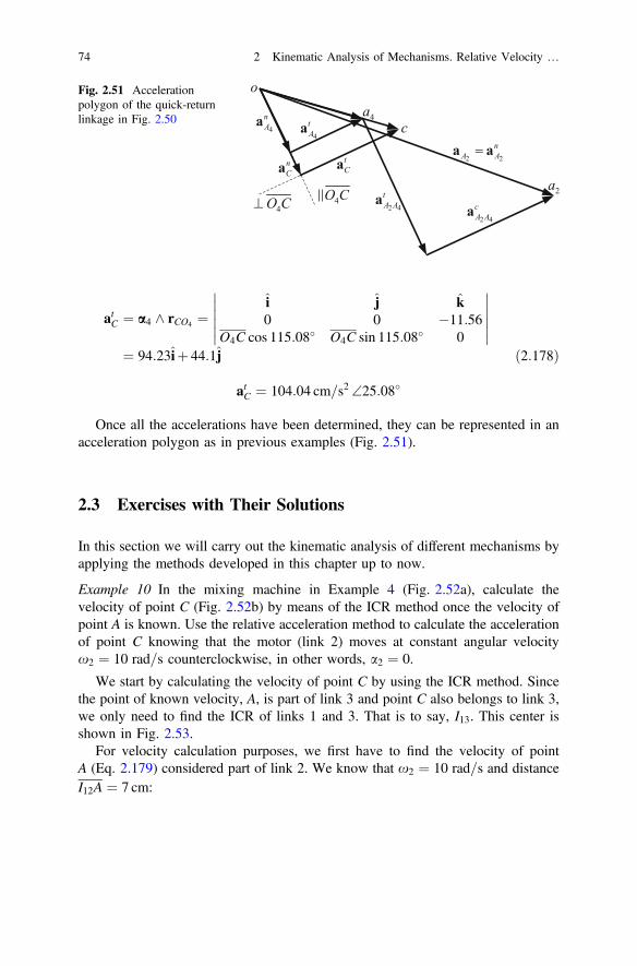
atC ¼ a4 ^ rCO4 ¼i j k0 0 �11:56

O4C cos 115:08� O4C sin 115:08� 0

��

¼ 94:23iþ 44:1j ð2:178Þ

atC ¼ 104:04 cm=s2 \25:08�

Once all the accelerations have been determined, they can be represented in anacceleration polygon as in previous examples (Fig. 2.51).

2.3 Exercises with Their Solutions

In this section we will carry out the kinematic analysis of different mechanisms byapplying the methods developed in this chapter up to now.

Example 10 In the mixing machine in Example 4 (Fig. 2.52a), calculate thevelocity of point C (Fig. 2.52b) by means of the ICR method once the velocity ofpoint A is known. Use the relative acceleration method to calculate the accelerationof point C knowing that the motor (link 2) moves at constant angular velocityx2 ¼ 10 rad=s counterclockwise, in other words, a2 ¼ 0.

We start by calculating the velocity of point C by using the ICR method. Sincethe point of known velocity, A, is part of link 3 and point C also belongs to link 3,we only need to find the ICR of links 1 and 3. That is to say, I13. This center isshown in Fig. 2.53.

For velocity calculation purposes, we first have to find the velocity of pointA (Eq. 2.179) considered part of link 2. We know that x2 ¼ 10 rad=s and distanceI12A ¼ 7 cm:

Fig. 2.51 Accelerationpolygon of the quick-returnlinkage in Fig. 2.50


vA ¼ x2I12A ¼ 70 cm=s ð2:179Þ

This same velocity associated to link 3 (Eq. 2.180) is:

vA ¼ x3I13I23 ) x3 ¼ vAI13I23

ð2:180Þ

To determine the angular velocity of link 3, we need to calculate distance I13I23(Eq. 2.181). We will make use of values l ¼ 32:47� and O4A ¼ 13:04 cm obtainedin Example 4:

I13I23 ¼ O4Asin l

¼ 24:289 cm ð2:181Þ

x3 ¼ vAI13I23

¼ 2:88 rad=s ð2:182Þ

Finally, we can calculate the velocity of point C (Eq. 2.183) knowing thath3 ¼ 122:47� and AC ¼ 21 cm:

(a) (b)Fig. 2.52 a Mixing machine.b Kinematic skeleton

Fig. 2.53 Calculation of thepoint C velocity using theICR method

2.3 Exercises with Their Solutions 75

vC ¼ x3I13C ¼ x3

ffiffiffiffiffiffiffiffiffiffiffiffiffiffiffiffiffiffiffiffiffiffiffiffiffiffiffiffiffiffiffiffiffiffiffiffiffiffiffiffiffiffiffiffiffiffiffiffiffiffiffiffiffiffiffiffiffiffiffiffiI13I23

2 þAC2 � 2 � I13I23 cos h3

qð2:183Þ

vC ¼ 114:4 cm=s

To calculate accelerations, we use the position and velocity results obtained inExample 4:

h3 ¼ 122:47� x3 ¼ 288 rad=s

vA ¼ 70j

vO3 ¼ vO3O4 ¼ �31:52i� 20:16j

vC ¼ 51:03iþ 102:45j

vO3A ¼ �31:68i� 20:16j

vCA ¼ 51:03iþ 32:45j

We start by calculating the acceleration of point O3 on link 3 (Eqs. 2.184 and2.185), which coincides with O4 at the instant being studied.

aO3 ¼ anA þ atA þ anO3A þ atO3A ð2:184Þ

aO3 ¼ anO4þ atO4

þ anO3O4þ atO3O4

þ acO3O4ð2:185Þ

In these equations, atA ¼ 0 due to the fact that the angular acceleration of link 2 iszero. Acceleration aO4 ¼ 0 because point O4 is on the frame. Finally, accelerationanO3O4

¼ 0 since the relative motion of point O3 with respect to link 4 follows astraight path.

The rest of the acceleration components (Eqs. 2.186–2.190) have the followingvalues:

anA ¼ x2 ^ vA ¼i j k0 0 100 70 0

�� ¼ �700i ð2:186Þ

anA ¼ 700 cm=s2 \180�

anO3A ¼ x3 ^ vO3A ¼i j k0 0 2:88

�31:68 �20:16 0

�� ¼ 58:06i� 91:24j ð2:187Þ

anO3A ¼ 108:15 cm=s2 \302:47�


atO3A ¼ a3 ^ rO3A ¼i j k0 0 a4

AO3 cos 122:47� AO3 sin 122:47� 0

�� ¼ �11a3i� 7a3j

ð2:188Þ

The relative acceleration component of will have the following values:

atO3O4¼ atO3O4

cos 122:47�iþ atO3O4sin 122:47� j ð2:189Þ

acO3O4¼ 2x3 ^ vO3O4 ¼ 2

i j k0 0 2:88

�31:52 49:53 0

�� ¼ �285:29i� 181:56j

ð2:190Þ

acO3O4¼ 338:16 cm=s2 \212:47�

Evening out the two vector equations that define the value of the acceleration ofpoint O3 and introducing the calculated values, we obtain Eq. (2.191):

ð�700iÞþ ð58:06i� 91:24jÞþ ð�11a3i� 7a3 jÞ¼ atO3O4

ð�0:54iþ 0:843jÞþ ð�285:29i� 181:56jÞð2:191Þ

By breaking up the components, we obtain Eq. (2.192):

�700þ 58:06� 11a3 ¼ 0:54atO3O4� 285:29

�91:24� 7a3 ¼ 0:843atO3O4� 181:56

�ð2:192Þ

This way, the angular acceleration of link 3 can be found, a3 ¼ �19:3 rad=s2, aswell as the magnitude of the relative tangential acceleration, atO3O4

¼ 267:37 cm=s2.Ultimately, we apply Eq. (2.193) to calculate the acceleration of point C:

aC ¼ anA þ atA þ anCA þ atCA ð2:193Þ

Relative accelerations (Eqs. 2.194 and 2.195) can be worked out as follows:

anCA ¼ x3 ^ vCA ¼i j k0 0 2:88

51:03 32:45 0

�� ¼ �93:46iþ 146:97j ð2:194Þ

atCA ¼ a3 ^ rCA ¼i j k0 0 �19:3

11:27 �17:71 0

�� ¼ �341:94i� 217:59j ð2:195Þ


Therefore, the acceleration of point C is Eq. (2.196):

aC ¼ ð�700iÞþ ð�93:46iþ 146:97jÞþ ð�341:94i� 217:59jÞ ð2:196Þ

aC ¼ �1135:4i� 70:62j ¼ 1137:6 cm=s2 \183:56�

Once the acceleration problem has been solved, we can represent the vectorsobtained and draw the acceleration polygon in Fig. 2.54:

Example 11 Figure 2.55a represents a mechanism that is part of a calculatingmachine that carries out multiplications and divisions. At the instant shown,knowing that O2A ¼ 1 cm, O2B ¼ 0:5 cm, input x ¼ 0:25 cm and link 2 moves withconstant angular velocity of x2 ¼ 1 rad=s counterclockwise, calculate:

1. Which constant value, k, the input has to be multiplied by to obtain output, y.That is to say, the value of constant k in equation y ¼ kx.

2. The velocity vector of points A, B, C and D using the relative velocity method.3. The acceleration vector of point C.4. The velocity vector of point C using the ICR method. Use the velocity of point

A calculated in question 2.

Fig. 2.54 Acceleration polygon of the mixing machine shown in Fig. (2.52)

(a)

(b)

Fig. 2.55 Calculating machine (a) and its velocity polygon (b) for x = 0.25 cm and x2 ¼ 1 rad=s


1. We start by calculating x and y (Eq. 2.197) in terms of h2.

x ¼ O2A sin h2

y ¼ O2B sin h2ð2:197Þ

Constant k will be given by Eq. (2.198):

k ¼ yx¼ O2A

O2B¼ 2 ð2:198Þ

2. Angle h2 needs to be determined to calculate the velocity of point A:

y ¼ kx ¼ 2 � 0:25 cm ¼ 0:5 cm ) h2 ¼ arcsin0:51

¼ 30�

We now define the relationship between the velocity of point A5 and the velocityof point A6 (Eq. 2.199), which coincides with it at that certain instant but belongs tolink 6:


This yields the following velocity values (Eqs. 2.200 and 2.201):

vA5 ¼ vA2 ¼ x2 ^ rAO2 ¼i j k0 0 1

1 cos 30� 1 sin 30� 0

�� ¼ �0:5iþ 0:866j ð2:200Þ

vA5 ¼ 1 cm=s\120�

A6 is a point on link 6 with straight horizontal motion. Relative motion of pointsA5 and A6 is also a straight movement but with vertical direction.

vA6 ¼ vA6 i

vA5A6 ¼ vA5A6 jð2:201Þ

We introduce these values in Eq. (2.199) and we obtain Eq. (2.202):

0:5iþ 0:866j ¼ vA6 iþ vA5A6 j ð2:202Þ


The unknowns can easily be determined by separating the components.

vA6 ¼ �0:5i ¼ 0:5 cm=s\180�

vA5A6 ¼ 0:866j ¼ 0:866 cm=s\90�

Link 6 moves with straight translational motion. Therefore, all its points have thesame velocity. Since point C belongs to this link, its velocity is:

vC ¼ vA6 ¼ �0:5i ¼ 0:5 cm=s\180�

To calculate the velocity of point D, we proceed in a similar way. We have tocalculate the velocity of point B4:

vB3 ¼ vB4 þ vB3B4 ð2:203Þ

In Eq. (2.203), the velocities are given by Eqs. (2.204) and (2.205):

vB3 ¼ x2 ^ rBO2 ¼i j k0 0 1

0:5 cos 300� 0:5 sin 300� 0

�� ¼ 0:43iþ 0:25j ð2:204Þ

vB3 ¼ 0:5 cm=s\30�

vB4 ¼ vB4 j

vB3B4 ¼ vB3B4 ið2:205Þ

Plugging these values into Eq. (2.203), we obtain Eq. (2.206):

0:43iþ 0:25j ¼ vB4 jþ vB3B4 i ð2:206Þ

From which we can calculate the following values:

vB4 ¼ 0:25j ¼ 0:25 cm=s\90�

vB3B4 ¼ 0:43i ¼ 0:43 cm=s\0�

Since point D belongs to link 4, which moves along a straight line, its velocitywill be the same as the point B4 velocity:

vD ¼ vB4 ¼ 0:25j ¼ 0:25 cm=s\90�

Once all the velocities have been determined, they can be represented in avelocity polygon (Fig. 2.55b).

3. To calculate the acceleration of point C, we start by defining Eq. (2.207), whichrelates the accelerations of point A5 on link 5 with A6 on link 6.


anA5þ atA5

¼ anA6þ atA6

þ anA5A6þ atA5A6

þ acA5A6ð2:207Þ

The values of the acceleration components Eq. (2.208) in Eq. (2.207) are:

anA5¼ anA2

¼ x2 ^ vA5 ¼i j k0 0 1

�0:5 0:866 0

�� ¼ �0:866i� 0:5j ð2:208Þ

atA5¼ atA2

¼ 0

anA6¼ 0

atA6¼ atA6

i

anA5A6¼ 0

atA5A6¼ atA5A6

j

acA5A6¼ 0

Introducing these values in Eq. (2.207), we obtain Eq. (2.209):

�0:866i� 0:5j ¼ atA6iþ atA5A6

j ð2:209Þ

Clearing the components, we obtain the values of the accelerations:

atA6¼ �0:866i ¼ 0:866 cm=s2 \180�

atA5A6¼ �0:5i ¼ 0:5 cm=s2 \270�

Once more, as point C belongs to link 6, which moves with straight translationalmotion, the acceleration of point C is the same as the acceleration of point A6:

aC ¼ aA6 ¼ �0:866i ¼ 0:866 cm=s2 \180�

Once the accelerations have been determined, they can be represented in anacceleration polygon (Fig. 2.56).

Fig. 2.56 Accelerationpolygon of points A2, A5, A6

and C in the mechanismshown in Fig. (2.55a)


4. To calculate the velocity of point C by means of the ICR method, we start bycalculating the relative instantaneous centers of rotation of link 1 (frame), link 2(the link point A belongs to) and link 6 (the link point C belongs to).

Once ICRs I12, I16 and I26 have been obtained (Fig. 2.57a), we can calculate thevelocity of I26. At the considered instant, I26 is part of links 2 and 6 simultaneously.As a point on link 2, it rotates about O2 and its velocity is Eq. (2.210):

vA ¼ x2I12A

vI26 ¼vAI12A

I12I26 ¼ 110:5 ¼ 0:5 cm=s ð2:210Þ

Moreover, I26 also belongs to link 6, which moves with linear translationalmotion and all its points have the same velocity. Hence, vC ¼ vI26 (Fig. 2.57a).

Example 12 Figure 2.58 represents a Scotch Yoke mechanism used in the assemblyline of a production chain. The lengths of the links are O2A ¼ 1m and O2B ¼ 1:2m.At the instant considered, angle h2 ¼ 60� and angular velocity x2 ¼ �1 rad=s(clockwise). Knowing that link 2 moves with constant velocity, calculate:

1. The acceleration of point C.2. The velocity of point C by using the ICR method when the velocity of point B is

known.

1. First of all, we make use of the vector (Eq. 2.211) to calculate the velocities:


(a)

(b)

Fig. 2.57 a Calculation of the velocity of point C with the ICR method using velocity vA2 .b Polygon to analyze ICRs positions


Next, we obtain the expressions of these components Eqs. (2.212)–(2.214). Westart by calculating vA3 (Eq. 2.212) knowing that O2A forms an angle of60� þ 90� ¼ 150� with the X-axis (Fig. 2.58a) and that x2 ¼ �1 rad=s clockwise.

vA3 ¼ vA2 ¼ x2 ^ rAO2 ¼i j k0 0 �1

1 cos 150� 1 sin 150� 0

�� ¼ 0:5iþ 0:866j

ð2:212Þ

vA3 ¼ vA2 ¼ 1m=s\60�

The trajectory of link 4 forms an angle of 180� � 10� ¼ 170� with the X-axis(Fig. 2.58a), thus:

vA4 ¼ vA4 cos 170�iþ vA4 sin 170

�j ¼ �0:985vA4 iþ 0:174vA4 j ð2:213Þ

The motion of A3 with respect to A4 follows a straight line that forms an angle of80� with the X-axis, consequently:

vA3A4 ¼ vA3A4 cos 80�iþ vA3A4 sin 80

� j ¼ 0:174vA3A4 iþ 0:985vA3A4 j ð2:214Þ

We plug these values into relative velocity (Eq. 2.211) and we obtainEq. (2.215):

ð0:5iþ 0:866jÞ ¼ ð�0:985vA4 iþ 0:174vA4 jÞþ ð0:174vA3A4 iþ 0:985vA3A4 jÞð2:215Þ

By separating the vector components, we find the system of algebraic equations(Eq. 2.216):

(a) (b)

Fig. 2.58 a Scotch Yoke mechanism. b Velocity polygon


0:5 ¼ �0:985vA4 þ 0:174vA3A4

0:866 ¼ 0:174vA4 þ 0:985vA3A4

�ð2:216Þ

In this system we can find the magnitude of the point A4 velocity,vA4 ¼ �0:34m=s, and the magnitude of the relative velocity, vA3A4 ¼ 0:94m=s.With these values, we can calculate the velocity vectors:

vA4 ¼ 0:335i� 0:059j ¼ 0:34m=s\350�

vA3A4 ¼ 0:163iþ 0:925j ¼ 0:94m=s\80�

Since all points on link 4 follow a straight path, the velocity of point C is thesame as the one of point A4:

vC ¼ vA4 ¼ 0:335i� 0:059j ¼ 0:34m=s\350�

Figure 2.58b shows the velocity polygon corresponding to these results.To calculate the acceleration, we apply Eq. (2.217):

aA3 ¼ aA4 þ aA3A4 ð2:217Þ

where the components of the accelerations (Eqs. 2.218–2.220) can be expressed as:

anA3¼ anA2

¼ x2 ^ vA3 ¼i j k0 0 �10:5 0:866 0

�� ¼ 0:866i� 0:5j ð2:218Þ

atA3¼ 0

anA4¼ 0

aA4 ¼ atA4¼ aA4 cos 170

�iþ aA4 sin 170� j ð2:219Þ

aA3A4 ¼ atA3A4¼ aA3A4 cos 80

�iþ aA3A4 sin 80� j ð2:220Þ

We obtain Eq. (2.221) plugging these values into relative acceleration(Eq. 2.217):

ð0:866i� 0:5jÞ ¼ ð�0:985aA4 iþ 0:174aA4 jÞþ ð0:174aA3A4 iþ 0:985aA3A4 jÞð2:221Þ

Separating the vector components (Eq. 2.222):

0:866 ¼ �0:985aA4 þ 0:174aA3A4

�0:5 ¼ 0:174aA4 þ 0:985aA3A4

�ð2:222Þ


Finally, solving the algebraic equation system, we obtain:

aA4 ¼ 0:926i� 0:163j ¼ 0:94m=s2 \350�

aA3A4 ¼ �0:059i� 0:335j ¼ 0:34m=s2 \260�

Since link 4 moves with translational motion without rotation, the acceleration ofpoint C is the same as the one of point A4:

aC ¼ aA4 ¼ 0:926i� 0:163j ¼ 0:94m=s2 \350�

We can see these results represented in the acceleration polygon in Fig. 2.59.

1. We now calculate the velocity of point C using the ICR method. Since theknown velocity belongs to a point in link 2 (point B) and the one we want to findcorresponds to a point of link 4 (point C), the relative ICRs of links 1, 2 and 4need to be determined. In other words, we need to determine ICRs I12, I14 andI24. Once the centers have been obtained (Fig. 2.60), we calculate the velocity ofI24. Point B rotates about point O2 with the following velocity:

vB ¼ x2I12B ¼ 1:2m=s

vI24 ¼vBI12B

I12I24 ¼ 1:21:2

O2A sin 20� ¼ 0:34m=s

Since all points in link 4 follow a straight path, instantaneous center I24 yieldsthe velocity of any point of link 4. The velocity of point C is:

vC ¼ vI24 ¼ 0:34m=s

Its direction is as shown in Fig. 2.60.

Example 13 Figure 2.61 represents a quick return mechanism that has the fol-lowing dimensions: O2O4 ¼ 25mm, O2A ¼ 30mm, AB ¼ 50mm, O4B ¼ O4C ¼45mm and CD ¼ 50mm. The angle between sides O4B and O4C of the triangle

Fig. 2.59 Accelerationpolygon of points A3, A4 andC of the Scotch Yokemechanism in Fig. (2.58a)


MBO4C is 90�. Calculate the velocity of point D of the slider when the position andvelocity of the input link are h2 ¼ 225� and x2 ¼ 80 rpm clockwise. Use the ICRmethod.

Consider that point D, of unknown velocity, is part of link 6 (it could also beconsidered part of link 5) and that point A, of known velocity, is part of link 2 (it isalso part of link 3). We have to find the relative ICRs of links 1, 2 and 6, that is,centers I12, I16 and I26.

Figure 2.62 shows the ICRs and the auxiliary lines used to find them. Beforestarting the calculation, we have to convert the velocity of the input link from rpminto rad/s (80 rpm ¼ 8:38 rad=s).

In order to obtain the velocity of point D graphically, we need to know thevelocity of point A (Eq. 2.223):

vA ¼ x2I12A ð2:223Þ

Figure 2.62 shows how is vI26 calculated graphically using vA. However, thisvelocity (Eq. 2.224) can also be obtained mathematically:

v26 ¼ x2I12I26 ð2:224Þ

Fig. 2.61 Quick-returnmechanism

Fig. 2.60 Calculation of the velocity of point C with the ICR method using velocity vB


Since link 6 is moving with non-angular velocity, all the points in this link havethe same velocity:

vD ¼ vI26 ¼ x2I12I26 ¼ 211:8mm=s ð2:225Þ

Its direction is shown in Fig. 2.62.

Example 14 The mechanism shown in Fig. 2.63 represents the second inversion ofa slider-crank mechanism where the slider follows a circular arc trajectory withradius R ¼ 24:4 cm. The mechanism has the following dimensions: O2P ¼ 10 cmand O2O4 ¼ 14:85 cm. Consider that link 2 rotates clockwise with a constantvelocity of x2 ¼ 12 rad=s clockwise and that h2 ¼ 180� at the instant considered.Find the velocity and acceleration of link 4. Point Q of link 4 and point P of link 2are superposed.

We start by solving the position problem using trigonometry (Eqs. 2.226–2.229). We apply the law of cosines to triangle MO4O2P:

O4P ¼ffiffiffiffiffiffiffiffiffiffiffiffiffiffiffiffiffiffiffiffiffiffiffiffiffiffiffiffiffiffiffiffiffiffiffiffiffiffiffiffiffiffiffiffiffiffiffiffiffiffiffiffiffiffiffiffiffiffiffiffiffiffiffiffiffiffiffiffiffiffiffiffiffiO2O4

2 þO2P2 � 2 O2O4 O2P cos 90�

q¼ 17:9 cm ð2:226Þ

Fig. 2.63 Invertedslider-crank mechanism withthe slider following a curvedpath. Point P on link 2 iscoincident with point Q onlink 4 at the studied instant

Fig. 2.62 Calculation of the velocity of point D with the ICR method knowing vA


We also know that:

O4P cosðh4 � 180�Þ ¼ O2P

h4 ¼ 180� þ arccos1017:9

¼ 236:06�ð2:227Þ

Applying the law of cosines to triangle MO4PC:

O4P2 ¼ R2 þR2 � 2R2 cosU

U ¼ arccos2R2 � O4P

2

2R2 ¼ 43:04�ð2:228Þ

2bþU ¼ 180� ) b ¼ 180� � U2

¼ 68:48� ð2:229Þ

In Fig. 2.63 we can observe that the normal direction to link 4 on point Q is NN 0.Its angle is defined by hNN 0 ¼ h4 � 180� þ b ¼ 124:54�. The tangential direction tolink 4 on point Q is defined by TT 0 and its angle is hTT 0 ¼ h4 � 180�

þ b� 90� ¼ 34:54�.Applying the relative velocity method to points P and Q (Eq. 2.230):

vP ¼ vQ þ vPQ ð2:230Þ

The absolute velocity of point P (Eq. 2.231), the extreme point of link 2, is:

vP ¼ x2 ^ rPO2 ¼i j k0 0 �12

10 cos 180� 10 cos 180� 0

�� ¼ 120j ð2:231Þ

vP ¼ 120 cm=s\90�

The direction of velocity vPQ is tangential to the trajectory followed by link 3when it slides inside the guide rail of link 4 (Eq. 2.232). Nevertheless, its magnitudewill be one of the unknowns of the problem.

vPQ ¼ vPQ cos hTT 0 iþ vPQ sin hTT 0 j ð2:232Þ

This relative velocity (Eq. 2.233) can also be expressed as the vector product ofthe angular velocity of radius R associated to slider movement and the vector thatgoes from the center of curvature C to point P:

vPQ ¼ xR ^ rPC ð2:233Þ


The velocity of point Q (Eq. 2.234) is:

vQ ¼ x4 ^ rQO4 ¼i j k

0 0 x4

17:9 cos 236:06�

17:9 sin 236:06�

0

��

¼ 14:85x4i� 10x4 j

ð2:234Þ

Substituting each vector in the relative velocity expression and separating itscomponents, we obtain the following system of two equations and two unknowns(Eq. 2.235), x4 and vPQ:

0 ¼ 14:85x4 þ 0:823vPQ120 ¼ �10x4 þ 0:567vPQ

�ð2:235Þ

x4 ¼ �5:94 rad=s

vPQ ¼ 106:96 cm=s

Hence, velocities vQ and vPQ are:

vQ ¼ �88:21iþ 59:4j ¼ 106:33 cm=s\146:06�

vPQ ¼ 88:1iþ 60:64j ¼ 106:96 cm=s\34:54�

Once the velocities have been obtained, the velocity polygon can be drawn(Fig. 2.64).

Once vector vPQ is defined, we have to calculate xR in Eq. (2.236). This valuewill be needed to solve the acceleration problem.

vPQ ¼ xR ^ rPC ¼i j k0 0 xR

R cosðhNN 0 þ 180�Þ R sinðhNN 0 þ 180�Þ 0

�� ð2:236Þ

88:1iþ 60:64j ¼ �RxR sin 304:54�iþRxR cos 304:54� j

Fig. 2.64 Velocity polygonof the mechanism shown inFig. (2.63)


Clearing, we obtain:

xR ¼ �88:1R sin 304:54�

¼ 4:38 rad=s

Finally, we can study the acceleration problem. The angular velocity of link 2 isconstant. Therefore, its angular acceleration (a2) is null. Defining the vectorexpression of the relative acceleration (Eq. 2.237) between P and Q:

aP ¼ aQ þ aPQ ð2:237Þ

anP þ atP ¼ anQ þ atQ þ anPQ þ atPQ þ acPQ ð2:238Þ

And analyzing each vector in Eq. (2.238), we obtain Eqs. (2.239)–(2.245):

anP ¼ x2 ^ vP ¼i j k0 0 �120 120 0

�� ¼ 1440i ð2:239Þ

atP ¼ a2 ^ rPO2 ¼ 0 ð2:240Þ

aP ¼ 1440i ¼ 1440 cm=s2 \0�

The normal acceleration of point Q (Eq. 2.241) is:

anQ ¼ x4 ^ vQ ¼i j k0 0 5:94

�88:21 59:4 0

�� ¼ 352:62iþ 523:97j ð2:241Þ

anQ ¼ 631:6 cm=s2 \56:06�

The tangential acceleration of point Q (Eq. 2.242) is:

atQ ¼ a4 ^ rQO4 ¼i j k0 0 a4

17:9 cos 236:06� 17:9 sin 236:06� 0

�� ¼ 14:85a4i� 10a4j

ð2:242Þ

The normal component of the acceleration of point P relative to point Q isEq. (2.243):

anPQ ¼ xR ^ vPQ ¼i j k0 0 4:38

88:1 60:64 0

�� ¼ �265:62iþ 385:9j ð2:243Þ


anPQ ¼ 468:1 cm=s2 \124:54�

This vector is perpendicular to velocity vPQ and it points towards the trajectorycurvature center followed by link 3 when it slides along the link 4, that is to say,from P to C. The tangential component of the acceleration of P relative toQ (Eq. 2.244) is:

atPQ ¼ aR ^ rPC ¼i j k0 0 aR

24:4 cos 304:54� 24:4 cos 304:54� 0

��

¼ 20:1aRiþ 13:83aR j ð2:244Þ

And the Coriolis component of the acceleration of P relative to Q (Eq. 2.245) is:

acPQ ¼ 2x4 ^ vPQ ¼ 2i j k0 0 �5:94

88:1 60:64 0

�� ¼ 720:45i� 1046:7j ð2:245Þ

acPQ ¼ 1270:7 cm=s2 \304:54�

Plugging these values into Eq. (2.238) and separating its components, we obtainthe system of two equations and two unknowns, aR and a4, Eq. (2.246).

ð1440iÞ ¼ ð352:62iþ 523:97jÞþ ð14:85a4i� 10a4 jÞþ ð�265:62iþ 385:9jÞþ ð20:1aRiþ 13:83aR jÞþ ð720:45i� 1046:7jÞ

1440 ¼ 352:62þ 14:85a4 � 265:62þ 20:1aR þ 720:45

0 ¼ 523:97� 10a4 þ 385:9þ 13:83aR � 1046:7

)ð2:246Þ

where:

a4 ¼ 14:77 rad=s2

aR ¼ 20:56 rad=s2

With these values we can calculate the tangential components of the accelerationof point Q relative to O4 and to P.

atQ ¼ 219:33i� 147:7j ¼ 264:38 cm=s2 \326:06�

atPQ ¼ 413:26iþ 284:34j ¼ 501:7 cm=s2 \34:54�

With these values, the acceleration polygon can be drawn (Fig. 2.65).


Example 15 Make a complete kinematic analysis of the shaft press mechanism inFig. 2.66, provided that: h2 ¼ 241� and x2 ¼ �10 rad=s clockwise constant.Piston 8 follows a trajectory along a vertical line that passes through O6. Thedimensions of the mechanism are: O2A ¼ 1:4 cm, AB ¼ 3:5 cm, O4B ¼ 1:4 cm,rO2 ¼ ð0; 0Þ cm, rO4 ¼ ð�3:1;�1:6Þ cm, BC ¼ 3:7 cm, CD ¼ 5 cm,O6D ¼ 1:2 cm, rO6 ¼ ð0;�2:8Þ cm, O6E ¼ 1:5 cm, w ¼ 67:5� and EF ¼ 2:3 cm.Use the relative velocity and acceleration methods.

Before we start to calculate velocities, it is necessary to solve the positionproblem. We will use the trigonometric method (Eqs. 2.247–2.266) developed inAppendix A for this purpose.

We start by studying the position of links 3 and 4 (Fig. 2.67).

Fig. 2.65 Accelerationpolygon of the mechanismshown in Fig. (2.63)

Fig. 2.66 Shaft pressmechanism


O2O4 ¼ffiffiffiffiffiffiffiffiffiffiffiffiffiffiffiffiffiffix2O4

þ y2O4

q¼

ffiffiffiffiffiffiffiffiffiffiffiffiffiffiffiffiffiffiffiffiffiffi3:12 þ 1:62

p¼ 3:49 cm ð2:247Þ

h1 ¼ 180� þ arctanyO4

xO4

¼ 207:3� ð2:248Þ

The application of the law of cosines to triangle MO2O4A yields:

O4A ¼ffiffiffiffiffiffiffiffiffiffiffiffiffiffiffiffiffiffiffiffiffiffiffiffiffiffiffiffiffiffiffiffiffiffiffiffiffiffiffiffiffiffiffiffiffiffiffiffiffiffiffiffiffiffiffiffiffiffiffiffiffiffiffiffiffiffiffiffiffiffiffiffiffiffiffiffiffiffiffiffiffiffiffiffiO2O4

2 þO2A2 � 2 O2O4 O2A cosðh2 � h1Þ

q¼ 2:54 cm ð2:249Þ

We also apply the law of sines to the same triangle:

O2A sinðh2 � h1Þ ¼ O4A sin a ð2:250Þ

a ¼ arcsin1:4 sin 33:7�

2:45¼ 18:47�

Hence:

b ¼ h1 � 180� � a ¼ 27:3� � 18:47� ¼ 8:83� ð2:251Þ

Next, we apply the law of cosines to triangle MO4AB:

O4B2 ¼

ffiffiffiffiffiffiffiffiffiffiffiffiffiffiffiffiffiffiffiffiffiffiffiffiffiffiffiffiffiffiffiffiffiffiffiffiffiffiffiffiffiffiffiffiffiffiffiffiffiffiffiffiffiffiffiffiffiffiffiffiO4A

2 þAB2 � 2 O4A AB cos/

qð2:252Þ

/ ¼ arccos2:452 þ 3:52 � 1:62

2 � 2:45 � 3:5 ¼ 23:81�

Thus:

h3 ¼ 180� þ bþ/ ¼ 180� þ 8:83� þ 23:81� ¼ 212:64� ð2:253Þ

Fig. 2.67 Calculation of theposition of links 3 and 4 withthe trigonometric method


Finally, we apply the law of sines to triangle MO4AB:

O4B sinð180� � dÞ ¼ AB sin/ ð2:254Þ

d ¼ 180� � arcsin3:2 sin 23:81�

1:6¼ 117:98�

This yields:

h4 ¼ 360� þ b� d ¼ 360� þ 8:83� � 117:98 ¼ 250:85� ð2:255Þ

Next, we study links 5 and 6 (Fig. 2.68).

O4O6 ¼ffiffiffiffiffiffiffiffiffiffiffiffiffiffiffiffiffiffiffiffiffiffiffiffiffiffiffiffiffiffiffiffiffiffiffiffiffiffiffiffiffiffiffiffiffiffiffiffiffiffiffiffiffiðxO4 � xO6Þ2 þðyO4 � yO6Þ2

q¼

ffiffiffiffiffiffiffiffiffiffiffiffiffiffiffiffiffiffiffiffiffiffi3:12 þ 1:22

p¼ 3:32 cm ð2:256Þ

h01 ¼ arctanyO4 � yO6

xO4 � xO6

¼ arctan�1:23:1

¼ 338:84� ð2:257Þ

We apply the law of cosines to triangle MO4O6C:

O6C ¼ffiffiffiffiffiffiffiffiffiffiffiffiffiffiffiffiffiffiffiffiffiffiffiffiffiffiffiffiffiffiffiffiffiffiffiffiffiffiffiffiffiffiffiffiffiffiffiffiffiffiffiffiffiffiffiffiffiffiffiffiffiffiffiffiffiffiffiffiffiffiffiffiffiffiffiffiffiffiffiffiffiffiffiffiffiffiffiffiffiffiffiffiffiffiffiffiffiffiffiffiO4C

2 þO4O62 � 2 O4O6 O4C cosðh4 þ 180� � h10 Þ

q¼ 3:99 cm

ð2:258Þ

We also apply the law of sines to the same triangle:

O4C sinðh4 þ 180� � h10 Þ ¼ O6C sin a ð2:259Þ

a ¼ arcsin2:1 sin 92:01�

3:99¼ 31:735�

b ¼ aþ 360� � h10 ¼ 31:735� þ 360� � 338:84� ¼ 52:895� ð2:260Þ

Fig. 2.68 Variables definedto calculate the position oflinks 5 and 6 with thetrigonometric method


Next, we apply the law of cosines to triangle MO6CD:

O6D2 ¼ O6C

2 þCD2 � 2 O6C CD cos/ ð2:261Þ

/ ¼ arccos3:992 þ 52 � 1:22

2 � 3:99 � 5 ¼ 8:32�

Thus:

h5 ¼ 360� � b� / ¼ 360� � 52:895� � 8:32� ¼ 298:8� ð2:262Þ

The application of the law of sines on triangle MO6CD yields:

O6D sinð180� � dÞ ¼ CD sin/ ð2:263Þ

d ¼ 180� � arcsin5 sin 8:32�

1:2¼ 142:92�

Thus:

h6 ¼ 180� � bþ d ¼ 180� � 52:895� þ 142:92� ¼ 270�

Finally, we will solve the position problem for links 7 and 8 (Fig. 2.69).

O6E sinw ¼ EF sin l ð2:264Þ

l ¼ arcsin1:5 sin 67:5�

2:3¼ 37:05�

Hence:

h7 ¼ 270� � l ¼ 232:95� ð2:265Þ

Projecting O6E and EF on the vertical axis, we obtain:

O6E coswþEF cos l ¼ FO6y ð2:266Þ

Fig. 2.69 Variables definedto calculate the position oflinks 7 and 8 using thetrigonometric method


FO6y ¼ 1:5 cos 67:5� þ 2:3 cos 37:05� ¼ 2:41 cm

The position of point F with respect to O2 will be given by Eq. (2.267):

FO2y ¼ FO6y þO6O2y ¼ �2:41� 2:8 ¼ �5:21 cm ð2:267Þ

Once the position of each link has been obtained, we can solve the velocityproblem. We start by analyzing the velocities of points A and B. The velocity ofpoint A (Eq. 2.268), which is the end of the crank (link 2), is:

vA ¼ x2 ^ rAO2 ¼i j k0 0 x2

O2A cos h2 O2A sin h2 0

�� ¼ 12:24i� 6:79j ð2:268Þ

vA ¼ 14 cm=s\331�

Taking into account that point A is also part of link 3, we can calculate thevelocity of any other point (point B) on the same link by means of the relativevelocity (Eq. 2.269):


The velocity of point B of link 4 (Eq. 2.270) is:

vB ¼ x4 ^ rBO4 ¼i j k0 0 x4

O4B cos h4 O4B sin h4 0

�� ¼ 1:511x4i� 0:525x4 j

ð2:270Þ

And the velocity of point B relative to point A (Eq. 2.271) is:


AB cos h3 AB sin h3 0

�� ¼ 1:888x3i� 2:947x3 j ð2:271Þ

Substituting these values in the relative velocity (Eq. 2.269) and separating thisequation into its components, we obtain Eq. (2.272):

ð1:511x4i� 0:525x4 jÞ ¼ ð12:24i� 6:79jÞþ ð1:888x3i� 2:947x3 jÞ

1:511x4 ¼ 12:24þ 1:888x3

�0:525x4 ¼ �6:79� 2:947x3

)ð2:272Þ


The solution of Eq. (2.272) is:

x3 ¼ �1:11 rad=s

x4 ¼ 6:71 rad=s

Using the angular velocities of links 3 and 4 we can now calculate vectors vB,vBA and vC (Eq. 2.273):

vB ¼ 10:17i� 3:55j ¼ 10:77 cm=s\340:85�

vBA ¼ �2:1iþ 3:27j ¼ 3:885 cm=s\122:6�

vC ¼ x4 ^ rCO4 ¼i j k

0 0 x4

O4C cosðh4 þ 180� Þ O4C sinðh4 þ 180

� Þ 0

��

¼ �13:31iþ 4:62j

ð2:273Þ

vC ¼ 14:1 cm=s\160:85�

We will continue the velocity analysis with points D and E. Assuming now thatpoint C belongs to link 5, we can calculate the velocity of point D of the same linkby means of the relative velocity (Eq. 2.274):

vD ¼ vC þ vDC ð2:274Þ

Hence, the velocity of point D of link 6 (Eq. 2.275) is:

vD ¼ x6 ^ rDO6 ¼i j k0 0 x6

O6D cos h6 O6D sin h6 0

�� ¼ �1:2x6i ð2:275Þ

The relative velocity of point D relative to point C (Eq. 2.276) can be expressedas:

vDC ¼ x5 ^ rDC ¼i j k0 0 x5

CD cos h5 CD sin h5 0

�� ¼ �4:382x5i� 2:409x5 j

ð2:276Þ

Plugging these values into the relative velocity (Eq. 2.274) and separating thecomponents, we obtain Eq. (2.277):


ð�1:2x6iÞ ¼ ð�13:31iþ 4:62jÞþ ð�4:382x5i� 2:409x5 jÞ

�1:2x6 ¼ �13:31� 4:382x5

0 ¼ 4:62� 2:409x5

�ð2:277Þ

where the values of the angular velocities can be obtained:

x5 ¼ �1:92 rad=s

x6 ¼ �18:09 rad=s

Therefore, the velocities of points D and E (Eq. 2.278) are:

vD ¼ �21:7i ¼ 21:71 cm=s\180�

vDC ¼ �8:41i� 4:625j ¼ 9:6 cm=s\208:8�

vE ¼ x6 ^ rEO6 ¼i j k

0 0 x6

O6E cosðh6 þwÞ O6E sinðh6 þwÞ 0

��

¼ �10:38i� 25:07j

ð2:278Þ

vE ¼ 27:13 cm=s\247:5�

Finally, to calculate the velocity of point F we use Eq. (2.279):

vF ¼ vE þ vFE ð2:279Þ

The velocity of point F of link 8 is a vector that has the direction of the Y -axissince the displacement of the piston follows a vertical trajectory (Eq. 2.280).Therefore, the velocity of point F can be expressed as:

vF ¼ vF j ð2:280Þ

The velocity of F relative to E is given by Eq. (2.281):

vFE ¼ x7 ^ rFE ¼i j k0 0 x7

EF cos h7 EF sin h7 0

�� ¼ 1:835x7i� 1:385x7 j ð2:281Þ

Plugging these values into Eq. (2.279) and separating its components, we obtainEq. (2.282):


ðvF jÞ ¼ ð�10:38i� 25:07jÞþ ð1:835x7i� 1:385x7 jÞ

0 ¼ �10:38þ 1:835x7

vF ¼ �25:07� 1:385x7

)ð2:282Þ

where the unknowns can easily be calculated.

x7 ¼ 5:65 rad=s

vF ¼ �32:91 cm=s

With these values vectors vF and vFE can be completely defined:

vF ¼ �32:91j ¼ 32:91 cm=s\270�

vFE ¼ 10:37i� 7:83j ¼ 12:995 cm=s\322:9�

Figure 2.70 shows the velocity polygon, which was constructed by drawing thevelocity vectors to scale. All the absolute velocities were drawn starting from thesame point, o, called the pole of velocities.

After solving the position and velocity problems, we can calculate the acceler-ations of the links of the mechanism. We will start by analyzing the acceleration ofpoints A and B.

The acceleration of point A (Eq. 2.283) is:

anA ¼ x2 ^ vA ¼i j k0 0 10

12:24 �6:79 0

�� ¼ 67:9iþ 122:4j ð2:283Þ

Fig. 2.70 Velocity polygonof the mechanism shown inFig. 2.66


atA ¼ 0

aA ¼ anA ¼ 67:9iþ 122:4j ¼ 140 cm=s2 \61�

The relationship between the accelerations of points A and B (Eq. 2.284) is:

anB þ atB ¼ anA þ atA þ anBA þ atBA ð2:284Þ

We continue by analyzing the rest of the vectors in Eq. (2.284). The normalcomponent of the acceleration of point B (Eq. 2.285) is:

anB ¼ x4 ^ vB ¼i j k0 0 x4

10:17 �3:55 0

�� ¼ 23:63iþ 68:05j ð2:285Þ

anB ¼ 72:04 cm=s2 \70:85�

The tangential component of the acceleration of point B (Eq. 2.286) is:

atB ¼ a4 ^ rBO4 ¼i j k0 0 a4


�� ¼ 1:511a4i� 0:5249a4 j

ð2:286Þ

The normal component of the acceleration of point B relative to pointA (Eq. 2.287) is:

anBA ¼ x3 ^ vBA ¼i j k0 0 x3

�2:1 3:27 0

�� ¼ 3:63iþ 2:326j ð2:287Þ

anBA ¼ 4:31 cm=s2 \32:64�

Finally, the tangential component of the acceleration of B relative toA (Eq. 2.288) is:


AB cos h3 AB sin h3 0

�� ¼ 1:888a3i� 2:947a3 j ð2:288Þ

Plugging each vector into Eq. (2.284) and projecting its components onto theX-axis and Y -axis, we obtain a system with two unknowns, a3 and a4, Eq. (2.289).


ð23:63iþ 68:05jÞþ ð1:511a4i� 0:5249a4 jÞ¼ ð67:9iþ 122:4jÞþ ð3:63iþ 2:326jÞþ ð1:888a3i� 2:947a3jÞ

23:63þ 1:511a4 ¼ 67:9þ 3:63þ 1:888a368:05� 0:5249a4 ¼ 122:4þ 2:326� 2:947a3

)ð2:289Þ

Solving this system, we obtain Eq. (2.290):

a3 ¼ 31:9 rad=s2

a4 ¼ 71:48 rad=s2

�ð2:290Þ

With these values we can calculate the absolute acceleration vectors of pointsB and C and the acceleration vector of point B with respect to point A (Eq. 2.291):

aB ¼ 131:67iþ 30:53j ¼ 135:16 cm=s2 \13:1�

aBA ¼ 63:85i� 91:69j ¼ 111:73 cm=s2 \304:85�

anC ¼ x4 ^ vC ¼i j k

0 0 6:71

�13:31 4:62 0

�� ¼ �31i� 89:31j

atC ¼ a4 ^ rCO4 ¼i j k

0 0 71:48

2:3 cos 70:85� 2:3 sin 70:85� 0

�� ¼ �15:53iþ 53:61j

aC ¼ anC þ atC ¼ �186:3i� 35:7j ¼ 189:68 cm=s2 \183:33� ð2:291Þ

We will continue by studying the accelerations of points D and E. The rela-tionship between the accelerations of points D and C is given by Eq. (2.292):

aD ¼ anD þ atD ¼ anC þ atC þ anDC þ atDC ð2:292Þ

The remaining vectors (Eqs. 2.293–2.295) in Eq. (2.292) are:

anD ¼ x6 ^ vD ¼i j k0 0 �18:09

�21:7 0 0

�� ¼ 392:7j

atD ¼ a6 ^ rDO6 ¼i j k0 0 a6

1:2 cos 270� 1:2 sin 270� 0

�� ¼ 1:2a6i


aD ¼ 1:2a6iþ 392:7j ð2:293Þ

atDC ¼ a5 ^ rDC ¼i j k0 0 a5

5 cos 298:8� 5 sin 298:8� 0

�� ¼ 4:38a5iþ 2:41a5 j

ð2:294Þ

anDC ¼ x5 ^ vDC ¼i j k0 0 �1:92

�8:41 �4:625 0

�� ¼ �8:88iþ 16:15j ð2:295Þ

Substituting these values in Eq. (2.292) and separating the resulting vectors intotheir components, we obtain Eq. (2.296):

ð1:2a6iþ 392:7jÞ ¼ ð�172:82i� 40:08jÞþ ð4:38a5iþ 2:41a5 jÞþ ð�8:88iþ 16:15jÞ

1:2a6 ¼ �172:82þ 4:38a5 � 8:88392:7 ¼ �40:08þ 2:41a5 þ 16:15

�ð2:296Þ

Solving the system, we obtain Eq. (2.297):

a5 ¼ 172:9 rad=s2

a6 ¼ 479:6 rad=s2

�ð2:297Þ

The acceleration vectors of points D and E with respect to the frame and theacceleration vector of point D relative to point C (Eq. 2.298) are:

aD ¼ 575:52iþ 392:7j ¼ 696:73 cm=s2 \34:3�

aDC ¼ 748:42iþ 432:84j ¼ 864:57 cm=s2 \30:04�

anE ¼ x6 ^ vE ¼i j k

0 0 �18:09

�10:38 �25:07 0

�� ¼ �453:52iþ 187:77j

atE ¼ a6 ^ rEO6 ¼i j k

0 0 479:6

1:5 cos 337:5� 1:5 sin 337:5� 0

�� ¼ 275:29iþ 664:73j

aE ¼ anE þ atE ¼ �178:2iþ 852:5j ð2:298Þ


aE ¼ 870:93 cm=s2 \101:8� ð2:299Þ

Finally, we need to find the acceleration in the crank-shaft mechanism formed bylinks 6, 7 and 8. We define acceleration vectors for point E (Eq. 2.300) and F oflink 7:

aF ¼ anF þ atF ¼ anE þ atE þ anFE þ atFE ð2:300Þ

where:

aF ¼ atF ¼ aF j ð2:301Þ

anFE ¼ x7 ^ vFE ¼i j k0 0

0

�� ¼ 44:24iþ 58:6j ð2:302Þ

atFE ¼ a7 ^ rFE ¼i j k0 0 a7

0

�� ¼ 1:836a7i� 1:386a7 j ð2:303Þ

Substituting the values of Eqs. (2.301)–(2.303) in the relative acceleration(Eq. 2.300) and breaking the resulting vector into its components, we obtain theequation system of two equations with two unknowns, a7 and aF , Eq. (2.304):

ðaF jÞ ¼ ð�178:2iþ 852:5jÞþ ð44:24iþ 58:6jÞþ ð1:836a7i� 1:386a7 jÞ

0 ¼ �178:2þ 44:24þ 1:836a7aF ¼ 852:5þ 58:6� 1:386a7

)ð2:304Þ

Solving the system we obtain:

a7 ¼ 72:96 rad=s2

aF ¼ 810 cm=s2

�The relative acceleration vector of point F with respect to point E is:

aFE ¼ 178:19i� 42:52j ¼ 183:19 cm=s2 \346:58�

Figure 2.71 represents the acceleration polygon built by drawing the absoluteacceleration vectors, all of them starting at the pole of accelerations. Relativeacceleration vectors are obtained by joining the extreme points of absolute accel-eration vectors. Student are recommended to do this exercise in order to betterunderstand vector directions in this problem.


Example 16 The mechanism in Fig. 2.72 is part of a calculating machine thatcarries out the “inverse” (1/y) arithmetic operation. Find the solution to the position,velocity and acceleration problems at the instant shown, knowing that the input isequal to y ¼ 1:87 cm and that link 4 moves with a constant linear velocity of0:5 cm=s in an ascending direction.

We start by solving the position problem using the trigonometric method(Eq. 2.305). The expressions are:

O2A sin h2 ¼ yO2A cos h2 ¼

ffiffiffi3

p�

ð2:305Þ

Therefore:

tan h2 ¼ yffiffiffi3

p ) h2 ¼ arctan1:87ffiffiffi

3p ¼ 47:19�

O2A ¼ ysin h2

¼ 1:87sin 47:19�

¼ 2:55 cm

Fig. 2.71 Acceleration polygon of the mechanism shown in Fig. 2.66


We analyze the position of point B (Eq. 2.306):

O2B sin h2 ¼ 1ffiffi3

p

O2B cos h2 ¼ x

)ð2:306Þ

From where we obtain:

O2B ¼ 1 ffiffiffi

3p

sin h2¼ 1

ffiffiffi3

p

sin 47:19�¼ 0:79 cm

So:

x ¼ O2B cos h2 ¼ 0:79 cos 47:19� ¼ 0:535 cm

It can be verified that the value of y is always the inverse value of x.Once the position of the links in the mechanism have been defined, we can solve

the velocity problem.Link 4 makes a translational motion and follows a vertical trajectory at a con-

stant velocity of 0:5 cm=s. Therefore, the velocity of point A of link 4 is:

vA ¼ 0:5j

Fig. 2.72 Calculating machine that carries out the “inverse” (x ¼ 1=y) arithmetic operation


Since point 4 is common to links 3 and 4, it can be denominated A3. Theexpression of the relative velocity of the two coincident points of links 2 and 3(Eq. 2.307) is:


The velocity of point A of link 2 (Eq. 2.308) is:

vA2 ¼ x2 ^ rAO2 ¼i j k

0 0 x2

2:55 cosðh2 þ 180�Þ 2:55 sinðh2 þ 180�Þ 0

��

¼ 1:87x2i� 1:73x2 j

ð2:308Þ

The direction of the velocity of point A3 with respect to point A2 (Eq. 2.309) isdefined by the direction in which link 3 slides over link 2:

vA3A2 ¼ vA3A2 cos 47:19�iþ vA3A2 sin 47:19

� j ð2:309Þ

Plugging these values into the relative velocity (Eq. 2.307) and separating theresulting vector into its components yields the system of two algebraic equationswith two unknowns, x2 and vA3A2 , Eq. (2.310):

0 ¼ 1:87x2 þ 0:679vA3A2

0:5 ¼ �1:73x2 þ 0:734vA3A2

�ð2:310Þ

Solving the system we obtain:

x2 ¼ �0:13 rad=svA3A2 ¼ 0:367 cm=s

�With these values we can calculate vectors vA2 and vA3A2 :

vA2 ¼ �0:2431iþ 0:2249j ¼ 0:331 cm=s\137:19�

vA3A2 ¼ 0:249iþ 0:269j ¼ 0:36 cm=s\47:19�

To find the velocity of links 5 and 6, we have to relate the velocities of the twocoincident points at B (Eq. 2.311) (one of link 2 and another of link 5):

vB5 ¼ vB2 þ vB5B2 ð2:311Þ

Since point B5 also belongs to link 6 and all the points in this link share the samevelocity with horizontal direction, we can assert that:

vB5 ¼ vB5 i


Therefore, the velocity of link 2 (Eq. 2.312) is:

vB2 ¼ x2 ^ rBO2 ¼i j k0 0 �0:13

O2B cos h2 O2B sin h2 0

�� ¼ 0:075i� 0:069j

ð2:312Þ

vB2 ¼ 0:102 cm=s\317:19�

The direction of vector vB5B2 is defined by the direction in which link 5 slidesover link 2 (Eq. 2.313):

vB5B2 ¼ vB5B2 cos h2iþ vB5B2 sin h2 j ¼ 0:679vB5B2 iþ 0:733vB5B2 j ð2:313Þ

Substituting the values obtained in Eq. (2.311) and separating the vectors intotheir components, we obtain Eq. (2.314):

vB5 ¼ 0:075þ 0:679vB5B2

0 ¼ �0:069þ 0:733vB5B2

�ð2:314Þ

From where we can calculate the magnitudes of vB5 and vB5B2 :

vB5 ¼ 0:139 cm=svB5B2 ¼ 0:094 cm=s

�With these values, we can define the velocity vectors:

vB5 ¼ 0:139i ¼ 0:139 cm=s\0�

vB5B2 ¼ 0:0639iþ 0:0688j ¼ 0:094 cm=s\47:19�

Finally, we solve the acceleration problem. We have to take into account that theacceleration of link 4 is null. The relative acceleration (Eqs. 2.315 and 2.316) of thetwo coincident points, A2 and A3, is:

aA3 ¼ aA2 þ aA3A2 ð2:315Þ

anA3þ atA3

¼ anA2þ atA2

þ anA3A2þ atA3A2

þ acA3A2ð2:316Þ

Since point A3 also belongs to link 4:

aA3 ¼ 0


The rest of the vectors in Eq. (2.316) are (Eqs. 2.317–2.321):

anA2¼ x2 ^ vA2 ¼

i j k0 0 �0:13

�0:2431 0:2249 0

�� ¼ 0:029iþ 0:031j ð2:317Þ

aA2 ¼ 0:043 cm=s2 \47:19�

atA2¼ a2 ^ rAO2 ¼

i j k0 0 a2

2:55 cosðh2 þ 180�Þ 2:55 sinðh2 þ 180�Þ 0

��

¼ 1:87a2i� 1:73a2 j ð2:318Þ

The relative motion between points A2 and A3 follows a straight-line trajectoryalong link 2. Therefore, the normal component of relative acceleration anA3A2

is zeroand the direction of the tangential component is defined by link 2:

anA3A2¼ 0 ð2:319Þ

atA3A2¼ aA3A2 cos h2iþ aA3A2 sin h2 j ð2:320Þ

The Coriolis component of the acceleration is given by:

acA3A2¼ 2x2 ^ vA3A2 ¼ 2

i j k0 0 �0:13

0:249 0:269 0

�� ¼ 0:07i� 0:0647j ð2:321Þ

Substituting the values obtained in Eq. (2.316) and separating the resultingvectors into their components yields (Eq. 2.322):

0 ¼ 0:029þ 1:87a2 þ 0:07þ 0:6796aA3A2

0 ¼ 0:031� 1:73a2 � 0:0647þ 0:7336aA3A2

�ð2:322Þ

a2 ¼ �0:0375 rad=s2

aA3A2 ¼ �0:0425 cm=s2

)

In order to calculate the absolute acceleration of point B of link 5 (B5), we useEqs. (2.323) and (2.324):

aB5 ¼ aB2 þ aB5B2 ð2:323Þ

anB5þ atB5

¼ anB2þ atB2

þ anB5B2þ atB5B2

þ acB5B2ð2:324Þ


We analyze the acceleration components in Eq. (2.324) starting with point B oflink 5 (Eq. 2.325). Since point B5 also belongs to link 6 and all the points in thislink follow a horizontal trajectory:

anB5¼ 0 ð2:325Þ

atB5¼ aBi ð2:326Þ

The acceleration components of point B of link 2 will be:

anB2¼ x2 ^ vB2 ¼

i j k0 0 �0:13

0:075 �0:069 0

�� ¼ �0:0089i� 0:0097j ð2:327Þ

anB2¼ 0:013 cm=s2 \227:19�

atB2¼ a2 ^ rBO2 ¼

i j k0 0 �0:0375

0:79 cos 47:19� 0:79 sin 47:19� 0

��

¼ 0:0217i� 0:02j ð2:328Þ

atB2¼ 0:0296 cm=s2 \317:19�

The relative motion of point B5 with respect to link 2 follows a straight trajectorydefined by link 2. Therefore, the normal component of the acceleration of point B5

relative to point B2 is zero and the direction of the tangential component is definedby link 2.

anB5B2¼ 0 ð2:329Þ

atB5B2¼ atB5B2

cos h2iþ atB5B2sin h2 j ð2:330Þ

The Coriolis component of the acceleration of point B5 with respect to point B2

can be calculated with the following expression:

acB5B2¼ 2x2 ^ vB5B2 ¼ 2

i j k0 0 �0:13

0:0639 0:0688 0

�� ¼ 0:0178i� 0:0166j

ð2:331Þ

acB5B2¼ 0:0243 cm=s2 \317:19�


Plugging the expression of these acceleration components Eqs. (2.325)–(2.331)into Eq. (2.324) and separating each vector into its x and y components, we obtainEq. (2.332):

aB5 ¼ �0:0089þ 0:0217þ 0:0178þ 0:6796atB5B2

0 ¼ �0:0097� 0:02� 0:0166þ 0:7336atB5B2

�ð2:332Þ

Solving the system, we find the unknowns:

aB5 ¼ 0:0734 cm=s2

atB5B2¼ 0:0631 cm=s2

�Hence, the acceleration of link 6 is given by:

a6 ¼ aB5 ¼ 0:0734i ¼ 0:0734 cm=s2 \0�


http://www.springer.com/978-3-319-31968-1

kinematic analysis of mechanisms. relative velocity and

Documents