kit - integral geometry and algebraic structures for …hug/media/90.pdfinstitut fur mathematik,...

Integral Geometry and Algebraic Structures forTensor Valuations

Andreas Bernig and Daniel Hug

Abstract In this survey, we consider various integral geometric formulas for tensor-valued valuations that have been obtained by different methods. Furthermore weexplain in an informal way recently introduced algebraic structures on the spaceof translation invariant, smooth tensor valuations, including convolution, product,Poincare duality and Alesker-Fourier transform, and their relation to kinematicformulas for tensor valuations. In particular, we describe how the algebraic viewpointleads to new intersectional kinematic formulas and substantially simplified Croftonformulas for translation invariant tensor valuations. We also highlight the connectionto general integral geometric formulas for area measures.

1 Introduction

An important part of integral geometry is devoted to the investigation of integrals(mean values) of the form ∫

Gϕ(K ∩ gL) µ(dg),

where K,L ⊂ Rn are sets from a suitable intersection stable class of sets, G is a groupacting on Rn and thus on its subsets, µ is a Haar measure on G, and ϕ is a functionalwith values in some vector space W . Common choices for W are the reals or thespace of signed Radon measures. Instead of the intersection, Minkowski additionis another natural choice for a set operation which has been studied. The principleaim then is to express such integrals by means of basic geometric functionals of K

Andreas BernigInstitut fur Mathematik, Goethe-Universitat Frankfurt, Robert-Mayer-Str. 10, 60054 Frankfurt,Germany, e-mail: [email protected],Daniel HugKarlsruhe Institute of Technology (KIT), Department of Mathematics, D-76128 Karlsruhe, Germany,e-mail: [email protected]

59

60 Andreas Bernig and Daniel Hug

and L. Depending on the specific framework, such as the class of sets or the type offunctional under consideration, different methods have been developed to establishintegral geometric formulas, ranging from classical convexity, differential geometry,geometric measure theory to the theory of valuations. The interplay between thetheory of valuations and integral geometry, although a classical topic in convexity,has been expanded and deepened considerably in recent years. In the present survey,we explore the integral geometry of tensor-valued functionals. This study suggestsand requires generalizations in the theory of valuations which are of independentinterest.

Therefore, we describe how some algebraic operations known for smooth transla-tion invariant scalar-valued valuations (product, convolution, Alesker-Fourier trans-form) can be extended to smooth translation invariant tensor-valued valuations.Although these extensions are straightforward to define, they encode various inte-gral geometric formulas for tensor valuations, like Crofton-type formulas, rotationsum formulas (also called additive kinematic formulas) and intersectional kinematicformulas. Even in the easiest case of translation invariant and O(n)-covariant tensorvaluations, explicit formulas are hard to obtain by classical methods. With the presentalgebraic approach, we are able to simplify the constants in Crofton-type formulas fortensor valuations, and to formulate a new type of intersectional kinematic formulasfor tensor valuations. For the latter we show how such formulas can be explicitlycalculated in the O(n)-covariant case. As an important byproduct, we compute theAlesker-Fourier transform on a certain class of smooth valuations, called sphericalvaluations. This result is of independent interest and is the technical heart of thecomputation of the product of tensor valuations.

2 Tensor Valuations

The present chapter is based on the general introduction to valuations in Chap. 1 andon the description and structural analysis of tensor valuations contained in Chap. 2.The algebraic framework for the investigation of scalar valuations, which has alreadyproved to be very useful in integral geometry, is outlined in Chap. 4. In these chaptersrelevant background information is provided, including references to previous work,motivation and hints to applications. The latter are also discussed in other parts ofthis volume, especially in Chaps. 10, 12 and 13.

Let us fix our notation and recall some basic structural facts. We will write V fora finite-dimensional real vector space. Sometimes we fix a Euclidean structure onV , which allows us to identify V with Euclidean space Rn. The space of compactconvex sets (including the empty set) is denoted by K (V ) (or K n if V = Rn).The vector space of translation invariant, continuous scalar valuations is denotedby Val(V ) (or simply by Val if the vector space V is clear from the context). Thesmooth valuations in Val(V ) constitute an important subspace for which we writeVal∞(V ); see Definition 4.5 and Remark ??, Definition 5.5 and Proposition 5.8, andSection 6.3. There is a natural decomposition of Val(V ) (and then also of Val∞(V ))

Integral Geometry and Algebraic Structures for Tensor Valuations 61

into subspaces of different parity and different degrees of homogeneity, hence

Val(V ) =n⊕

m=0ε=±

Valεm(V ),

if V has dimension n, and similarly

Val∞(V ) =n⊕

m=0ε=±

Valε,∞m (V );

see Sects. 1.4, 4.1 and Theorem 5.1.Our main focus will be on valuations with values in the space of symmetric

tensors of a given rank p ∈ N0, for which we write Symp Rn or simply Symp if theunderlying vector space is clear from the context (resp., Symp V in case of a generalvector space V ). Here we deviate from the notation Tp used in Chaps. 1 and 2. Thespaces of symmetric tensors of different ranks can be combined to form a gradedalgebra in the usual way. By a tensor valuation we mean a valuation on K (V ) withvalues in the vector space of tensors of a fixed rank, say Symp(V ). For the space oftranslation invariant, continuous tensor valuations with values in Symp(V ) we writeTValp(V ); cf. the notation in Chapters 4, 6 and Definition 5.38. This vector spacecan be identified with Val(V )⊗ Symp(V ) (or Val⊗Symp, for short). If we restrictto smooth tensor valuations, we add the superscript ∞, that is TValp,∞(V ). It is clearthat McMullen’s decomposition extends to tensor valuations, hence

TValp(V ) =n⊕

m=0ε=±

TValp,εm (V ),

if dim(V ) = n. The corresponding decomposition is also available for smooth tensor-valued valuations or valuations covariant (or invariant) with respect to a compactsubgroup G of the orthogonal group which acts transitively on the unit sphere. Thevector spaces of tensor valuations satisfying an additional covariance condition withrespect to such a group G is finite-dimensional and consists of smooth valuationsonly (cf. Example 4.6 and Theorem 5.15). In the following, we will only considerrotation covariant valuations (see Chapter 2).

2.1 Examples of Tensor Valuations

In the following, we mainly consider translation invariant tensor valuations. However,we start with recalling general Minkowski tensors, which are translation covariantbut not necessarily translation invariant. For Minkowski tensors, and hence for allisometry covariant continuous tensor valuations, we first state a general Crofton


formula. The major part of this contribution is then devoted to translation invariant,rotation covariant, continuous tensor valuations. In this framework, we explain howalgebraic structures can be introduced and how they are related to Crofton formulasas well as to additive and intersectional kinematic formulas. Crofton formulas fortensor-valued curvature measures are the subject of Chap. ??.

For k ∈ {0, . . . , n − 1} and K ∈ K n, let Λ0(K, ·), . . . ,Λn−1(K, ·) denote thesupport measures associated with K (see Sect. 1.3). They are Borel measures onΣ n := Rn × Sn−1 which are concentrated on the normal bundle nc K of K. Let κndenote the volume of the unit ball and ωn = nκn the volume of its boundary, theunit sphere. Using the support measures, we recall from Sects. 1.3 or 2.1 that theMinkowski tensors are defined by

Φr,sk (K) :=

1r!s!

ωn−k

ωn−k+s

∫Σn

xrusΛk(K, d(x, u)),

for k ∈ {0, . . . , n− 1} and r, s ∈ N0, and

Φr,0n (K) :=

1r!

∫K

xr dx.

In addition, we define Φr,sk := 0 for all other choices of indices. Clearly, the tensor

valuations Φ0,sk and Φ

0,0n , which are obtained by choosing r = 0, are translation

invariant. However, these are not the only translation invariant examples, since e.g.Φ

1,1k−1, for k ∈ {1, . . . , n}, also satisfies Φ

1,1k−1(K + t) = Φ

1,1k−1(K) for all K ∈ K n

and t ∈ Rn.Further examples of continuous, isometry covariant tensor valuations are obtained

by multiplying the Minkowski tensors with powers of the metric tensor Q and bytaking linear combinations. As shown by Alesker [1, 2], no other examples exist (seealso Theorem 2.5). In the following, we write

Φsk(K) : = Φ

0,sk (K) =

1s!

ωn−k

ωn−k+s

∫Σn

usΛk(K, d(x, u))

=

(n− 1

k

)1

ωn−k+ss!

∫Sn−1

us Sk(K, du),

for k ∈ {0, . . . , n− 1}, where we used the kth area measure Sk(K, ·) of K, a Borelmeasure on Sn−1 defined by

Sk(K, ·) :=nκn−k(n

k

) Λk(K,Rn × ·).

In addition, we define Φ0n := Vn and Φ s

n := 0 for s > 0. The normalization is suchthat Φ0

k = Vk, for k ∈ {0, . . . , n}, where Vk is the kth intrinsic volume. Clearly, thetensor valuations QiΦ s

k , for k ∈ {0, . . . , n} and i, s ∈ N0, are continuous, translationinvariant, O(n)-covariant, homogeneous of degree k and have tensor rank 2i + s.We have Φ s

n ≡ 0 for s 6= 0, and Φ s0(K) is independent of K. Hence, we usually


exclude these trivial cases. Apart from these, Alesker showed that for each fixedk ∈ {1, . . . , n− 1} the valuations

QiΦ

sk , i, s ∈ N0, 2i + s = p, s 6= 1,

form a basis of the vector space of all continuous, translation invariant, O(n)-covarianttensor valuations of rank p which are homogeneous of degree k. The fact that thesevaluations span the corresponding vector space is implied by [1, Prop. 4.9] (and[2]), the proof is based in particular on basic representation theory. A result ofWeil [17, Thm. 3.5] states that differences of area measure of order k, for any fixedk ∈ {1, . . . , d − 1}, are dense in the vector space of differences of finite, centeredBorel measures on the unit sphere. From this the asserted linear independence of thetensor valuations can be inferred. We also refer to Sect. 6.5 where the present case isdiscussed as an example of a very general representation theoretic theorem.

The situation for general tensor valuations (which are not necessarily translationinvariant) is more complicated. As explained in Chap. 2, the valuations QiΦ

r,sk

span the corresponding vector space, but there exist linear dependences betweenthese functionals. Although all linear relations are known and the dimension of thecorresponding vector space (for fixed rank and degree of homogeneity) has beendetermined, the situation here is not perfectly understood.

In the following, it will often (but not always) be sufficient to neglect the metrictensor powers Qi and just consider the tensor valuations Φ s

k , since the metric tensorcommutes with the algebraic operations to be considered.

2.2 Integral Geometric Formulas

Let A(n, k), for k ∈ {0, . . . , n}, denote the affine Grassmannian of k-flats in Rn, andlet µk denote the motion invariant measure on A(n, k) normalized as in [13, 14]. TheCrofton formulas to be discussed below relate the integral mean∫

A(n,k)Φ

r,sj (K ∩ E) µk(dE)

of the tensor valuation Φr,sj (K ∩ E) of the intersection of K with flats E ∈ A(n, k) to

tensor valuations of K. Guessing from the scalar case, one would expect that onlytensor valuations of the form QiΦ

r′,s′n−k+ j(K) are required. It turns out, however, that

for general r the situation is more involved.The following Crofton formulas for Minkowski tensors have been established in

[7]. Since Φr,sj (K ∩ E) = 0 if k < j, we only have to consider the cases where k ≥ j.

We start with the basic case k = j, in which the Crofton formula has a particularlysimple form.

Theorem 2.1. For K ∈ K n, r, s ∈ N0 and 0 ≤ k ≤ n− 1,


∫A(n,k)

Φr,sk (K ∩ E) µk(dE) =

αn,k,s Qs2 Φ

r,0n (K), if s is even,

0, if s is odd,

where

αn,k,s :=1

(4π)s2( s

2

)!

Γ( n

2

)Γ( n−k+s

2

)Γ( n+s

2

)Γ( n−k

2

) .This result essentially follows from Fubini’s theorem, combined with a relation

due to McMullen, which connects the Minkowski tensors of K∩E and the Minkowskitensors of K ∩ E, defined with respect to the flat E as the ambient space (see (4) fora precise statement).

The main case j < k is considered in the next theorem.

Theorem 2.2. Let K ∈ K n and k, j, r, s ∈ N0 with 0 ≤ j < k ≤ n− 1. Then∫A(n,k)

Φr,sj (K ∩ E) µk(dE)

=b s

2 c

∑z=0

χ(1)n, j,k,s,zQ

zΦ

r,s−2zn+ j−k(K) +

b s2 c−1

∑z=0

χ(2)n, j,k,s,zQ

z

×s−2z−1

∑l=0

(2πlΦ r+s−2z−l,l

n+ j−k−s+2z+l(K)− QΦr+s−2z−l,l−2n+ j−k−s+2z+l(K)

), (1)

where χ(1)n, j,k,s,z and χ

(2)n, j,k,s,z are explicitly known constants.

The constants χ(1)n, j,k,s,z and χ

(2)n, j,k,s,z only depend on the indicated lower indices. It

is remarkable that they are independent of r. Moreover, the right-hand side of thisCrofton formula also involves other tensor valuations than Φ

r′,s′n−k+ j(K). For instance,

in the special case where n = 3, k = 2, j = 0, r = 1 and s = 2, Theorem 2.2 yieldsthat ∫

A(3,2)Φ

1,20 (K ∩ E) µ2(dE) =

13

Φ1,21 (K) +

124π

QΦ1,01 (K) +

16

Φ2,10 (K).

It can be shown that it is not possible to write Φ2,10 as a linear combination of Φ

1,21

and QΦ1,01 , which are the only other Minkowski tensors of rank 3 and homogeneity

degree 2.The explicit expressions obtained for the constants χ

(1)n, j,k,s,z and χ

(2)n, j,k,s,z in [7]

require a multiple (five-fold) summation over products and ratios of binomial coeffi-cients and Gamma functions. Some progress which can be made in simplifying thisrepresentation is described in Chap. ??.

Since the tensor valuations on the right-hand side of the Crofton formula (1) arenot linearly independent, the specific representation is not unique. Using the linearrelation due to McMullen, the result can also be expressed in the form

Integral Geometry and Algebraic Structures for Tensor Valuations 65∫A(n,k)

Φr,sj (K ∩ E) µk(dE)

=b s

2 c

∑z=0

χ(1)n, j,k,s,zQ

zΦ

r,s−2zn+ j−k(K) +

b s2 c−1

∑z=0

χ(2)n, j,k,s,zQ

z

× ∑l≥s−2z

(QΦ

r+s−2z−l,l−2n+ j−k−s+2z+l(K)− 2πlΦ r+s−2z−l,l

n+ j−k−s+2z+l(K))

(2)

with the same constants as before. From (2) we now deduce the Crofton formulafor the translation invariant tensor valuations Φ s

j . For r = 0, the sum ∑l≥s−2z on theright-hand side of (2) is non-zero only if l = s − 2z. Therefore, after some indexshift (and discussion of the ‘boundary cases’ z = 0 and z = b s

2c), we obtain

∫A(n,k)

Φsj(K ∩ E) µ

nk (dE) =

b s2 c

∑z=0

χ(∗)n, j,k,s,zQ

zΦ

s−2zn+ j−k(K) (3)

for j < k, where

χ(∗)n, j,k,s,z = χ

(1)n, j,k,s,z + χ

(2)n, j,k,s,z−1 − 2π(s− 2z)χ(2)

n, j,k,s,z.

Since the right-hand side of (3) is uniquely determined by the left-hand side andthe tensor valuations on the right-hand side are linearly independent, the constantχ(∗)n, j,k,s,z is uniquely determined. Using the expression which is obtained for χ

(∗)n, j,k,s,z

from the constants χ(1)n, j,k,s,z and χ

(2)n, j,k,s,z provided in [7], it seems to be a formidable

task to get a reasonably simple expression for this constant. If j = k, then Theorem2.1 shows that (3) remains true if we define χn,k,k,s,b s

2 c := αn,k,s if s is even, and aszero in all other cases. As we will see, the approach of algebraic integral geometry to(3) will reveal that χ

(∗)n, j,k,s,z has indeed a surprisingly simple expression.

To compare the algebraic approach with the one used in [7], and extended totensorial curvature measures in Chap. ??, we point out that the result of Theorem2.2 is complemented by and in fact is based on an intrinsic Crofton formula, wherethe tensor valuation Φ

r,sj (K ∩ E) is replaced by Φ

r,sj,E(K ∩ E). The latter is the tensor

valuation of the intersection K ∩ E, determined with respect to E as the ambientspace but considered as a tensor in Rn(see Section ?? or [7] for an explicit definition).The two tensors are connected by the relation

Φr,sj (K ∩ E) = ∑

m≥0

Q(E⊥)m

(4π)mm!Φ

r,s−2mj,E (K ∩ E), (4)

due to McMullen [11, Theorem 5.1] (see also [7]), where Q(E⊥) is the metric tensorof the linear subspace orthogonal to the direction space of E but again considered as atensor in Rn, that is, Q(E⊥) = e2

k+1 + . . .+ e2n, where ek+1, . . . , en is an orthonormal

basis of E⊥. Note that for s = 0 we get Φr,0j (K ∩ E) = Φ

r,0j,E(K ∩ E), since the


intrinsic volumes and the suitably normalized curvature measures are independent ofthe ambient space.

The intrinsic Crofton formula for∫A(n,k)

Φr,sj,E(K ∩ E) µk(dE)

has the same structure as the extrinsic Crofton formula stated in Theorem 2.2, but theconstants are different. Apart from reducing the number of summations required fordetermining the constants, progress in understanding the structure of these (intrinsicand extrinsic) integral geometric formulas can be made by localizing the Minkowskitensors. This is the topic of Chapter ??.

Crofton and intersectional kinematic formulas for Minkowski tensors Φr,sj with

s = 0 are special cases of corresponding (more general) integral geometric formulasfor curvature measures. For example, we have∫

A(n,k)Φ

r,0j (K ∩ E) µk(dE) = an jk Φ

r,0n+ j−k(K) (5)

and ∫Gn

Φr,0j (K ∩ gM) µ(dg) =

n

∑k= j

an jk Φr,0n+ j−k(K)Vk(M), (6)

where Gn is the Euclidean motion group, µ is the suitably normalized Haar measureand the (simple) constants an jk are known explicitly. Therefore, we focus on the cases 6= 0 (and r = 0) in the following.

A close connection between Crofton formulas and intersectional kinematic formu-las follows from Hadwiger’s general integral geometric theorem (see [14, Theorem5.1.2]). It states that for any continuous valuation ϕ on the space of convex bodiesand for all K,M ∈ K n, we have∫

Gn

ϕ(K ∩ gM) µ(dg) =n

∑k=0

∫A(n,k)

ϕ(K ∩ E) µk(dE)Vk(M). (7)

Hence, if a Crofton formula for the functional ϕ is available, then an intersectionalkinematic formula is an immediate consequence. This statement includes also tensor-valued functionals, since (7) can be applied coordinate-wise. In particular, this showsthat (6) can be obtained from (5). In the same way, Theorem 2.2 and the special caseshown in (3) imply kinematic formulas for intersections of convex bodies, one fixedthe other moving. Thus, for instance, we obtain

∫Gn

Φsj(K ∩ gM) µ(dg) =

b s2 c

∑z=0

n

∑k= j

χ(∗)n, j,k,s,z Qz

Φs−2zn+ j−k(K)Vk(M). (8)

These results are related to and in fact inspired general integral geometric formulasfor area measures (see [10]). The starting point is a local version of Hadwiger’sgeneral integral geometric theorem for measure-valued valuations. To state it, let


M+(Sn−1) be the cone of non-negative measures in the vector space M (Sn−1) offinite Borel measures on the unit sphere.

Theorem 2.3. Let ϕ : K n → M+(Sn−1) be a continuous and additive mappingwith ϕ( /0, ·) = 0 (the zero measure). Then, for K,M ∈ K n and Borel sets A ⊂ Sn−1,∫

Gn

ϕ(K ∩ gM,A) µ(dg) =n

∑k=0

[Tn,kϕ(K, ·)](A)Vk(M), (9)

with (the Crofton operator) Tn,k : M+(Sn−1)→M+(Sn−1) given by

Tn,kϕ(K, ·) :=∫

A(n,k)ϕ(K ∩ E, ·) µk(dE), k = 0, . . . , n.

We want to apply this result to area measures of convex bodies, hence we need aCrofton formula for area measures. The statement of such a Crofton formula is basedon Fourier operators Ip, for p ∈ {−1, 0, 1, . . . , n}, which act on C∞ functions on Sn−1.For f ∈ C∞(Sn−1), let fp be the extension of f to Rn \ {0} which is homogeneous ofdegree−n+p, and let fp be the distributional Fourier transform of fp. For 0 < p < n,the restriction Ip( f ) of fp to the unit sphere is again a smooth function. Let H n

sdenote the space of spherical harmonics of degree s. Recall that a spherical harmonicof degree s is the restriction to the unit sphere of a homogeneous polynomial p ofdegree s on Rn which satisfies ∆ p = 0 (and hence is called harmonic), where ∆ isthe Laplace operator. We refer to [13] for more information on spherical harmonics.Since Ip intertwines the group action of SO(n), we have Ip( fs) = λs(n, p) fs forfs ∈H n

s and some λs(n, p) ∈ C. It is known that

λs(n, p) = πn2 2p is

Γ( s+p

2

)Γ( s+n−p

2

) .Note that λs(n, p) is purely imaginary if s is odd, and real if s is even. See [10] fora summary of the main properties of this Fourier operator and [9, 8] for a detailedexposition.

Using the connection to mean section bodies (see [8]) and the Fourier operatorsIp, the following Crofton formula for area measures has been established in [10,Theorem 3.1].

Theorem 2.4. Let 1 ≤ j < k ≤ n and K ∈ K n. Then∫A(n,k)

S j(K ∩ E, ·) µk(dE) = a(n, j, k)I jIk− jSn+ j−k(−K, ·) (10)

with

a(n, j, k) :=j

2nπ(n+k)/2(n + j − k)Γ ( k+1

2 )Γ (n− j)

Γ ( n+12 )Γ (k − j)

.

Let I∗ be the reflection operator (I∗ f )(u) = f (−u), u ∈ Sn−1, for a function fon the unit sphere. The operator Tn, j,k := a(n, j, k)I jIk− jI∗, for 1 ≤ j < k ≤ n, and


the identity operator Tn, j,n act as linear operators on M (Sn−1) and can be used toexpress (10) in the form∫

A(n,k)S j(K ∩ E, ·) µk(dE) = Tn, j,kSn+ j−k(K, ·). (11)

This is also true for k = j < n if we define

Tn, j, jSn(K, ·) :=(

n− 1j

)−1ωn− j

ωnVn(K)σ ,

where σ is spherical Lebesgue measure. Combining equations (9) and (11), we obtaina kinematic formula for area measures. Using again the operator Tn, j,k, it can bestated in the form∫

Gn

S j(K ∩ gM,A) µ(dg) =n

∑k= j

[Tn, j,kSn+ j−k(K, ·)](A)Vk(M),

for j = 1, . . . , n − 1. Since the Fourier operators act as multiplier operators onspherical harmonics, it follows that Theorem 2.4 can be rewritten in the form∫

A(n,k)

∫Sn−1

fs(u) S j(K ∩ E, du) µk(dE)

= as(n, j, k)∫Sn−1

fs(u) Sn+ j−k(K, du), (12)

where fs ∈H ns and as(s, j, k) := a(n, j, k)bs(n, j, k) with

bs(n, j, k) := 2kπ

nΓ

(s+ j

2

)Γ

(s+k− j

2

)Γ

(s+n− j

2

)Γ

(s+n−k+ j

2

) .In addition to Crofton and intersectional kinematic formulas, there is another clas-

sical type of integral geometric formula. Since they involve rotations and Minkowskisums of convex bodies, it is justified to call them rotation sum formulas. Let SO(n)denote the group of rotations and let ν denote the Haar probability measure on thisgroup. A general form of such a formula can again be stated for area measures. LetK,M ∈ K n be convex bodies and let α, β ⊂ Sn−1 be Borel sets. Then [13, Theorem4.4.6] can be written in the form∫

SO(n)

∫Sn−1

1α(u)1β (ρ−1u) S j(K + ρM, du) ν(dρ)

=1

ωn

j

∑k=0

(jk

)Sk(K,α)S j−k(M, β ). (13)

More generally, by the inversion invariance of the Haar measure ν , by basic mea-sure theoretic extension arguments, and by an application of (13) to the coordinate


functions of an arbitrary continuous function f : Sn−1 × Sn−1 → Syms1 ⊗Syms2 ,for given s1, s2 ∈ N0, we obtain∫

SO(n)

∫Sn−1

f (u, ρu) S j(K + ρ−1M, du) ν(dρ)

=1

ωn

j

∑k=0

(jk

) ∫(Sn−1)2

f (u, v)(Sk(K, ·)× S j−k(M, ·)

)(d(u, v)).

To simplify constants, we define

φsk (K) :=

∫Sn−1

us Sk(K, du). (14)

Choosing f (u, v) = us1 ⊗ vs2 , we thus get∫SO(n)

(id⊗s1 ⊗ ρ⊗s2)φ s1+s2

j (K + ρ−1M) ν(dρ)

=∫

SO(n)

∫Sn−1

us1 ⊗ (ρu)s2 S j(K + ρ−1M, du) ν(dρ)

=1

ωn

j

∑k=0

(jk

) ∫(Sn−1)2

us1 ⊗ vs2(Sk(K, ·)× S j−k(M, ·)

)(d(u, v)), (15)

and hence∫SO(n)

(id⊗s1 ⊗ ρ⊗s2)φ s1+s2

j (K + ρ−1M) ν(dρ) =

1ωn

j

∑k=0

(jk

)φ

s1k (K)⊗ φ

s2j−k(M).

Up to the different normalization, this is the additive kinematic formula for tensorvaluations stated in [6, Theorem 5]. In particular,

∫SO(n)

φsj (K + ρM) ν(dρ) =

1ωn

j

∑k=0

(jk

)φ

sk (K)S j−k(M),

where Si(M) := Si(M,Sn−1) = nκn−i(n

i

)−1Vi(M).In the following section, we develop basic algebraic structures for tensor valuations

and provide applications to integral geometry. From this approach, we will obtaina Crofton formula for the tensor valuations Φ s

k , but also for another set of tensorvaluations, denoted by Ψ s

k , for which the Crofton formula has ‘diagonal form’.Moreover, we will study more general intersectional kinematic formulas than the oneconsidered in (8) and describe the connection between intersectional and additivekinematic formulas. In the course of our analysis, we determine Alesker’s Fourieroperator for spherical valuations, that is, valuations obtained by integration of aspherical harmonic (or, more generally, any smooth spherical function) against anarea measure.


3 Algebraic Structures on Tensor Valuations

Recall that Val = Val(Rn) denotes the Banach space of translation invariant continu-ous valuations on V = Rn, and Val∞ = Val∞(Rn) is the dense subspace of smoothvaluations; see Chapters 4 and 5 for more information. In this section, we first dis-cuss the extension of basic operations and transformations from scalar valuations totensor-valued valuations. The scalar case is described in Chap. 4.

In the following, we usually work in Euclidean space Rn with the Lebesguemeasure and the volume functional Vn on convex bodies. Since some of the resultsare also stated in invariant terms, we write vol for a volume measure on V , that is,a choice of a translation invariant locally finite Haar measure on an n-dimensionalvector space V . Of course, in case V = Rn we always use Vn as a specific choice ofthe restriction of a volume measure vol to K n (the corresponding choice is made forV = Rn × Rn).

3.1 Product

Existence and uniqueness of the product of smooth valuations is provided by thefollowing result; see also Sect. 4.2 for the more general construction of an exteriorproduct between smooth scalar-valued valuations on possibly different vector spaces.

Proposition 2.5. Let φ1, φ2 ∈ Val∞ be smooth valuations on Rn given by

φi(K) = vol(K + Ai), K ∈ K n,

where A1,A2 ∈ K n are smooth convex bodies with positive Gauss curvature atevery boundary point. Let ∆ : Rn → Rn × Rn be the diagonal embedding. Then

φ1 · φ2(K) := vol(∆K + A1 × A2), K ∈ K n,

extends by continuity and bilinearity to a product on Val∞.

The product is compatible with the degree of a valuation (i.e., if φi has degree ki,then φ1 · φ2 has degree k1 + k2 if k1 + k2 ≤ n), and more generally with the action ofthe group GL(n).

We can extend the product component-wise from smooth scalar-valued valuationsto smooth tensor-valued valuations. To see this, let V be a finite-dimensional vectorspace, V = Rn say, and s1, s2 ∈ N0. Let Φi ∈ TValsi,∞(V ) for i = 1, 2. Letw1, . . . ,wm be a basis of Syms1V , and let u1, . . . , ul be a basis of Syms2V . Thenthere are φi,ψ j ∈ Val∞(V ), i ∈ {1, . . . ,m} and j ∈ {1, . . . , l}, such that

Φ1(K) =m

∑i=1

φi(K)wi and Φ2(K) =l

∑j=1

ψ j(K)u j


for K ∈ K (V ). Now we would like to define (omitting the obvious ranges of theindices)

(Φ1 ·Φ2) (K) := ∑i, j(φi · ψ j)(K)wiu j.

The dot on the right-hand side is the product of the smooth valuations φi,ψ j, andwiu j ∈ Syms1+s2V denotes the symmetric tensor product of the symmetric tensorswi ∈ Syms1V and u j ∈ Syms2V .

Let us verify that this definition is independent of the chosen bases. For this,let w′i = ∑ j ci jw j with some invertible matrix (ci j), and let u′i = ∑ j ei ju j with aninvertible matrix (ei j).

IfΦ1(K) = ∑

iφ′i (K)w′i = ∑

iφi(K)wi,

then a comparison of coefficients yields that φ ′i = ∑ j c jiφ j, where (c ji) denotes thematrix inverse. Similarly, from

Φ2(K) = ∑i

ψ′j(K)u′i = ∑

iψi(K)ui,

we conclude that ψ ′i = ∑ j e jiψ j, where (e ji) denotes the matrix inverse. Therefore,we have

∑i, j(φ ′i · ψ ′j)w′iu′j = ∑

i, j,b1,b2

(∑

a1,b1

ca1iφa1 · e

b1 jψb1

)∑

a2,b2

cia2wa2e jb2ub2

= ∑a1,a2,b1,b2

(∑i, j

ca1icia2eb1 je jb2

)︸︷︷︸

=δa1a2 δ

b1b2

(φa1 · ψb1)wa2 · ub2

= ∑a,b(φa · ψa)wa · ub,

which proves the asserted independence of the representation.Thus, recalling that TValsm(V ) denotes the vector space of translation invariant

continuous valuations on K (V ) which are homogeneous of degree m and take valuesin the vector space Syms V of symmetric tensors of rank s over V , and that TVals,∞m (V )is the subspace consisting of the smooth elements of this vector space, we have

Φ1 ·Φ2 ∈ TVals1+s2,∞k+l (V ), k + l ≤ n,

for Φ1 ∈ TVals1,∞k (V ), Φ2 ∈ TVals2,∞

l (V ) and k, l ∈ {0, . . . , n}.A similar description and similar arguments can be given for the operations

considered in the following subsections.


3.2 Convolution

Similarly as for the product of valuations, an explicit definition of the convolution oftwo valuations is given only for a suitable subclass of valuations (cf. Sect. 4.3).

Proposition 2.6. Let φ1, φ2 ∈ Val∞ be smooth valuations on Rn given by

φi(K) = vol(K + Ai),

where A1,A2 are smooth convex bodies with positive Gauss curvature at everyboundary point. Then

φ1 ∗ φ2(K) := vol(K + A1 + A2),

extends by continuity and bilinearity to a product (which is called convolution) onVal∞.

Written in invariant terms, the convolution is a bilinear map

Val∞(V )⊗ Dens(V ∗)× Val∞(V )⊗ Dens(V ∗)→ Val∞(V )⊗ Dens(V ∗),

where Dens(V ∗) is the one-dimensional space of translation invariant, locally finitecomplex-valued Haar measures (Lebesgue measures, see Sect. 4.3) on the dual spaceV ∗. It is compatible with the action of the group GL(n) and with the codegree of avaluation (i.e., if φi has degree ki, then φ1 ∗ φ2 has degree k1 + k2 − n if k1 + k2 ≥ n).

The convolution can be extended component-wise to a convolution on the spaceof translation invariant smooth tensor valuations. Hence we have

Φ1 ∗Φ2 ∈ TVals1+s2,∞k+l−n (V ), k + l ≥ n,

for Φ1 ∈ TVals1,∞k (V ), Φ2 ∈ TVals2,∞

l (V ) and k, l ∈ {0, . . . , n}. This is analogous tothe definition and computation in the previous subsection.

3.3 Alesker-Fourier Transform

Alesker introduced an operation on smooth valuations, now called Alesker-Fouriertransform (cf. Sect. 4.4). It is a map F : Val∞(Rn)→ Val∞(Rn) which reverses thedegree of homogeneity, that is,

F : Val∞k (Rn)→ Val∞n−k(Rn),

and which transforms product into convolution of smooth valuations, more precisely,we have

F(φ1 · φ2) = F(φ1) ∗ F(φ2). (16)


On valuations which are smooth and even, the Alesker-Fourier transform caneasily be described in terms of Klain functions as follows. Let φ ∈ Val∞,+

k (Rn) (thespace of smooth and even valuations which are homogeneous of degree k). Then therestriction of φ to a k-dimensional subspace E is a multiple Klφ (E) of the volume,and the resulting function (Klain function) Klφ determines φ . Then

KlFφ (E) = Klφ (E⊥)

for every (n− k)-dimensional subspace E.As an example (and consequence of the relation to Klain functions), the intrinsic

volumes satisfyF(Vk) = Vn−k, (17)

where V0, . . . ,Vn denote the intrinsic volumes on K n.The description in the odd case is more involved and it is preferable to describe it

in invariant terms (i.e., without referring to a Euclidean structure).Let V be an n-dimensional real vector space. Then

F : Val∞k (V )→ Val∞n−k(V )⊗ Dens(V ∗),

where Dens denotes the one-dimensional space of densities (Lebesgue measures).This map commutes with the action of GL(V ) on both sides. Applying it twice (andusing the identification Dens(V ∗)⊗ Dens(V ) ∼= C), it satisfies the Plancherel typeformula

(F2φ)(K) = φ(−K).

Working again on Euclidean space V = Rn, we can extend the Alesker-Fouriertransform component-wise to a map F : TVals,∞ → TVals,∞ such that

F : TVals,∞k → TVals,∞n−k.

It is not an easy task to determine the Fourier transform of valuations other than theintrinsic volumes.

3.4 Example: Intrinsic Volumes

As an example, let us compute the Alesker product of intrinsic volumes V0, . . . ,Vn inRn. We complement the definition of the intrinsic volumes by Vl := 0 for l < 0. Letvol = Vn denote the volume measure on K n.

Recall Steiner’s formula (1.16) which states that

vol(K + rB) =n

∑i=0

Vn−i(K)κiri, r ≥ 0.


Now we fix r ≥ 0 and s ≥ 0 and define the smooth valuations φ1(K) := vol(K + rB)and φ2(K) := vol(K + sB). Then

φ1 ∗ φ2(K) = vol(K + rB + sB) = vol(K + (r + s)B) =n

∑k=0

Vn−k(K)κk(r + s)k,

hence

φ1 ∗ φ2 =n

∑i, j=0

Vn−i− jκi+ j

(i + j

i

)ris j.

On the other hand, since φ1 = ∑ni=0 Vn−iκiri and φ2 = ∑

ni=0 Vn−iκisi, we obtain

φ1 ∗ φ2 =n

∑i, j=0

Vn−i ∗Vn− jκiκ jris j.

Now we compare the coefficient of ris j in these equations and get

Vn−i− jκi+ j

(i + j

i

)= Vn−i ∗Vn− jκiκ j.

Writing i instead of n− i and j instead of n− j, we obtain

Vi ∗Vj =

[2n− i− j

n− i

]Vi+ j−n, (18)

where we used the flag coefficient[nk

]:=(

nk

)κn

κkκn−k, k ∈ {0, . . . , n}.

Taking Alesker-Fourier transform on both sides yields

Vi ·Vj =

[i + j

i

]Vi+ j. (19)

The computation of convolution and product of tensor valuations follows thesame scheme: first one computes the convolution of tensor valuations, which canbe considered easier. Then one applies the Alesker-Fourier transform to obtain theproduct. However, in the tensor-valued case it is much harder to write down theAlesker-Fourier transform in an explicit way. This step is the technical heart of ourapproach.


3.5 Poincare Duality

The product of smooth translation invariant valuations as well as the convolutionboth satisfy a version of Poincare duality, which moreover are identical up to a sign.

To state this more precisely, recall that the vector spaces Valk = Valk(Rn), k ∈{0, n}, are one-dimensional and spanned by the Euler-characteristic χ = V0 and thevolume functional Vn = vol, that is, Val0 ∼= R · χ and Valn ∼= R · vol. We denote byφ0, φn ∈ R the component of φ ∈ Val of degree 0 and n, respectively.

Proposition 2.7. The pairings

Val∞k ×Val∞n−k → R, (φ1, φ2) 7→ (φ1 · φ2)n,

andVal∞k ×Val∞n−k → R, (φ1, φ2) 7→ (φ1 ∗ φ2)0,

are perfect, that is, the induced maps

pdm, pdc : Val∞k → Val∞,∗n−k

are injective with dense image. Moreover,

pdc =

{pdm on Val+k .

−pdm on Val−k .

To illustrate this proposition and to highlight the difference between the twopairings, let us compute them on an easy example. Let φi(K) := vol(K + Ai),where Ai, i ∈ {1, 2}, are smooth convex bodies with positive Gauss curvature. Thenφ1 ∗ φ2(K) = vol(K + A1 + A2), and hence (φ1 ∗ φ2)0 = vol(A1 + A2).

On the other hand, φ1 · φ2(K) = vol2n(∆K + A1 × A2). Using Fubini’s theorem,one rewrites this as

φ1 · φ2(K) =∫Rn

φ2((x− A1) ∩ K) dx.

Taking for K a large ball reveals that (φ1 · φ2)n = φ2(−A1) = vol(A2 − A1). IfA1 = −A1, then φ1 is even and both pairings agree indeed.

The extension of Poincare duality to tensor-valued valuations is postponed toSect. 4.1 where it is required for the description of the relation between additive andintersectional kinematic formulas for tensor valuations.

3.6 Explicit Computations in the O(n)-Equivariant Case

In this subsection, we outline the explicit computation of product, convolution andAlesker-Fourier transform in the O(n)-equivariant case. Depending on the situation,


we will either use the basis consisting of the tensor valuations QiΦ s−2ik or the basis

consisting of the tensor valuations QiΨ s−2ik . The latter are defined in the following

proposition.

Proposition 2.8. The following statements hold.

(i) For 0 ≤ k < n and s 6= 1, define

Ψs

k := Φsk +

b s2 c

∑j=1

(−1) jΓ ( n−k+s2 )Γ ( n

2 + s− 1− j)

(4π) j j!Γ ( n−k+s2 − j)Γ ( n

2 + s− 1)Q j

Φs−2 jk

and let Ψ 0n := Φ0

n . Then Ψ sk is the trace free part of Φ s

k . In particular, Ψ sk ≡ Φ s

kmod Q.

(ii) For 0 ≤ k < n and s 6= 1, Φ sk can be written in terms of Ψ s′

k as

Φsk = Ψ

sk +

b s2 c

∑j=1

Γ( n−k+s

2

)Γ ( n

2 + s− 2 j)

(4π) j j!Γ ( n−k+s2 − j)Γ ( n

2 + s− j)Q j

Ψs−2 j

k .

The inversion which is needed to derive (ii) from (i) can be accomplished with thehelp of Zeilberger’s algorithm.

The first and easier step in the explicit calculations of algebraic structures fortensor valuations is to compute the convolution of two tensor valuations. Since Φ s

k issmooth (i.e., each component is a smooth valuation), we may write

Φsk(K) =

∫nc(K)

ωk,s,

where ωk,s is a smooth (n − 1)-form on the sphere bundle Rn × Sn−1 with valuesin Syms Rn. Next, for valuations represented by differential forms, there is an easyformula for the convolution, which involves only some linear and bilinear operations(a kind of Hodge star and a wedge product). The resulting formula states that, fork, l ≤ n with k + l ≥ n and s1, s2 6= 1, we have

Φs1k ∗Φ

s2l =

ωs1+s2+2n−k−l

ωs1+n−kωs2+n−l

(n− k)(n− l)2n− k − l

·

·(

2n− k − ln− k

)(s1 + s2

s1

)(s1 − 1)(s2 − 1)

1− s1 − s2Φ

s1+s2k+l−n,

or, using the normalization (14) which is more convenient for this purpose,

φs1k ∗ φ

s2l = n

(k+ln

)(k+lk

) (s1 − 1)(s2 − 1)1− s1 − s2

φs1+s2k+l−n.

The computation of the Alesker-Fourier transform of tensor valuations is the mainstep and will be explained in the next subsection. For 0 ≤ k ≤ n and s 6= 1, the resultis


F(Ψ sk ) = is Ψ

sn−k,

F(Φ sk) = is

b s2 c

∑j=0

(−1) j

(4π) j j!Q j

Φs−2 jn−k .

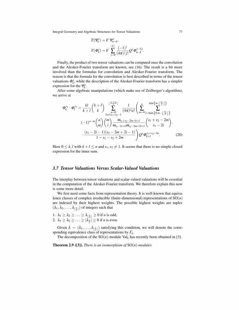
Finally, the product of two tensor valuations can be computed once the convolutionand the Alesker-Fourier transform are known, see (16). The result is a bit moreinvolved than the formulas for convolution and Alesker-Fourier transform. Thereason is that the formula for the convolution is best described in terms of the tensorvaluations Φ s

k , while the description of the Alesker-Fourier transform has a simplerexpression for the Ψ s

k .After some algebraic manipulations (which make use of Zeilberger’s algorithm),

we arrive at

Φs1k ·Φ

s2l =

klk + l

(k + l

k

) b s1+s22 c

∑a=0

2a6=s1+s2−1

1(4π)aa!

(a

∑m=0

min{m,b s12 c}

∑i=max{0,m−b s2

2 c}

(−1)a−m(

am

)(mi

)ωs1+s2−2m+k+l

ωs1−2i+kωs2−2m+2i+l

(s1 + s2 − 2m

s1 − 2i

)·

· (s1 − 2i− 1)(s2 − 2m + 2i− 1)1− s1 − s2 + 2m

)Qa

Φs1+s2−2ak+l . (20)

Here 0 ≤ k, l with k + l ≤ n and s1, s2 6= 1. It seems that there is no simple closedexpression for the inner sum.

3.7 Tensor Valuations Versus Scalar-Valued Valuations

The interplay between tensor valuations and scalar-valued valuations will be essentialin the computation of the Alesker-Fourier transform. We therefore explain this nowis some more detail.

We first need some facts from representation theory. It is well-known that equiva-lence classes of complex irreducible (finite-dimensional) representations of SO(n)are indexed by their highest weights. The possible highest weights are tuples(λ1, λ2, . . . , λb n

2 c) of integers such that

1. λ1 ≥ λ2 ≥ . . . ≥ λb n2 c ≥ 0 if n is odd,

2. λ1 ≥ λ2 ≥ . . . ≥ |λ n2| ≥ 0 if n is even.

Given λ = (λ1, . . . , λb n2 c) satisfying this condition, we will denote the corre-

sponding equivalence class of representations by Γλ .The decomposition of the SO(n)-module Valk has recently been obtained in [3].

Theorem 2.9 ([3]). There is an isomorphism of SO(n)-modules


Valk ∼=⊕

λ

Γλ ,

where λ ranges over all highest weights such that |λ2| ≤ 2, |λi| 6= 1 for all i andλi = 0 for i > min{k, n−k}. In particular, these decompositions are multiplicity-free.

Let Γ be an irreducible representation of SO(n) and Γ ∗ its dual. The space of k-homogeneous SO(n)-equivariant Γ -valued valuations (i.e., maps Φ : K → Γ suchthat Φ(gK) = gΦ(K) for all g ∈ SO(n)) is (Valk⊗Γ )SO(n) = HomSO(n)(Γ

∗,Valk).By Theorem 2.9, Γ ∗ appears in the decomposition of Valk precisely if Γ ap-pears, and in this case the multiplicity is 1. By Schur’s lemma it follows thatdim(Valk⊗Γ )SO(n) = 1 in this case.

Let us construct the (unique up to scale) equivariant Γ -valued valuation explicitly.Denote by Valk(Γ ) the Γ -isotypical summand, which is isomorphic to Γ since Valkis multiplicity free.

Let φ1, . . . , φm be a basis of Valk(Γ ). These elements play two different roles:first we can look at them as valuations, i.e., elements of Valk. Second, we may thinkof φ1, . . . , φm as basis of the irreducible representation Γ . The action of SO(n) onthis basis is given by

gφi = ∑j

c ji (g)φ j,

where (c ji (g))i, j is a matrix depending on g. The map g 7→ (c j

i (g))i, j is a homomor-phism of Lie groups SO(n)→ GL(m).

Let φ ∗1 , . . . , φ ∗m be the dual basis of Γ ∗. Then

gφ∗i = ∑

j(c j

i (g))−t

φ j = ∑j

cij(g−1)φ j,

Using the double role played by the φi mentioned above, we set

Φ(K) := ∑i

φi(K)φ ∗i ∈ Γ∗. (21)

We claim that Φ is an O(n)-equivariant valuation with values in Γ ∗. Indeed, wecompute


Φ(gK) = ∑i

φi(gK)φ ∗i

= ∑i(g−1

φi)(K)φ ∗i

= ∑i, j

c ji (g−1)φ j(K)φ ∗i

= ∑j

φ j(K)∑i

c ji (g−1)φ ∗i

= ∑j

φ j(K)gφ∗j

= g(Φ(K)).

Conversely, we now start with an equivariant Γ ∗-valued continuous translationinvariant valuation Φ of degree k. Let w1, . . . ,wm be a basis of Γ ∗. Then we maylook at the components of Φ , i.e., we decompose

Φ(K) = ∑i

φi(K)wi

with φi ∈ Valk. Let the action of SO(n) on Γ ∗ be given by

gwi = ∑j

a ji (g)w j.

We have

Φ(gK) = ∑i

φi(gK)wi = ∑i(g−1

φi)(K)wi,

g(Φ(K)) = ∑j

φ j(K)gw j = ∑i, j

φ j(K)aij(g)wi.

Comparing coefficients yields g−1φi = ∑ j aij(g)φ j, or

gφi = ∑j

aij(g−1)φ j.

This shows that the subspace of Valk spanned by φ1, . . . , φm is isomorphic to Γ .In summary, we have shown the following fact.

Each SO(n)-irreducible representation Γ appearing in the decomposition of Valkcorresponds to the (unique up to scale) Γ ∗-valued continuous translation invari-ant valuation Φ from (21). Conversely, the coefficients of a Γ ∗-valued continuoustranslation invariant valuation span a subspace of Valk isomorphic to Γ .

Let us now discuss the special case of symmetric tensor valuations. The SO(n)-representation space Syms is (in general) not irreducible. Indeed, the trace maptr : Syms → Syms−2 commutes with SO(n), hence its kernel is an invariant subspace.


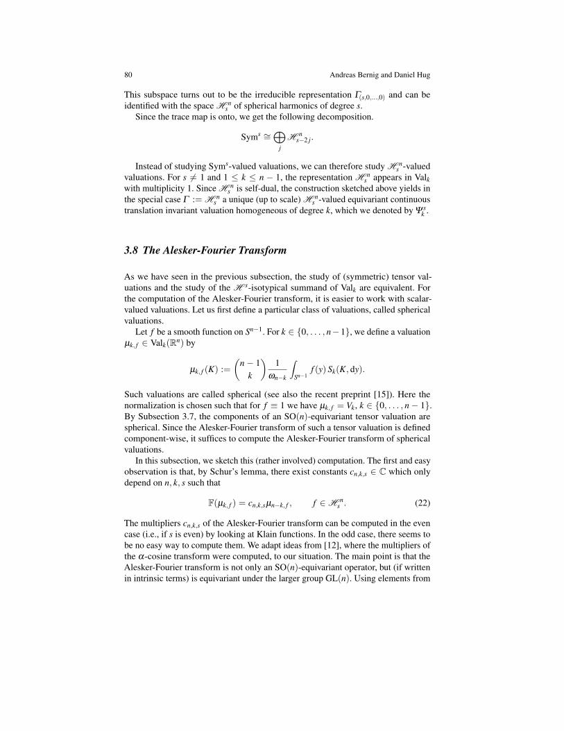
This subspace turns out to be the irreducible representation Γ(s,0,...,0) and can beidentified with the space H n

s of spherical harmonics of degree s.Since the trace map is onto, we get the following decomposition.

Syms ∼=⊕

j

H ns−2 j.

Instead of studying Syms-valued valuations, we can therefore study H ns -valued

valuations. For s 6= 1 and 1 ≤ k ≤ n − 1, the representation H ns appears in Valk

with multiplicity 1. Since H ns is self-dual, the construction sketched above yields in

the special case Γ := H ns a unique (up to scale) H n

s -valued equivariant continuoustranslation invariant valuation homogeneous of degree k, which we denoted by Ψ s

k .

3.8 The Alesker-Fourier Transform

As we have seen in the previous subsection, the study of (symmetric) tensor val-uations and the study of the H s-isotypical summand of Valk are equivalent. Forthe computation of the Alesker-Fourier transform, it is easier to work with scalar-valued valuations. Let us first define a particular class of valuations, called sphericalvaluations.

Let f be a smooth function on Sn−1. For k ∈ {0, . . . , n−1}, we define a valuationµk, f ∈ Valk(Rn) by

µk, f (K) :=(

n− 1k

)1

ωn−k

∫Sn−1

f (y) Sk(K, dy).

Such valuations are called spherical (see also the recent preprint [15]). Here thenormalization is chosen such that for f ≡ 1 we have µk, f = Vk, k ∈ {0, . . . , n− 1}.By Subsection 3.7, the components of an SO(n)-equivariant tensor valuation arespherical. Since the Alesker-Fourier transform of such a tensor valuation is definedcomponent-wise, it suffices to compute the Alesker-Fourier transform of sphericalvaluations.

In this subsection, we sketch this (rather involved) computation. The first and easyobservation is that, by Schur’s lemma, there exist constants cn,k,s ∈ C which onlydepend on n, k, s such that

F(µk, f ) = cn,k,sµn−k, f , f ∈H ns . (22)

The multipliers cn,k,s of the Alesker-Fourier transform can be computed in the evencase (i.e., if s is even) by looking at Klain functions. In the odd case, there seems tobe no easy way to compute them. We adapt ideas from [12], where the multipliers ofthe α-cosine transform were computed, to our situation. The main point is that theAlesker-Fourier transform is not only an SO(n)-equivariant operator, but (if writtenin intrinsic terms) is equivariant under the larger group GL(n). Using elements from


the Lie algebra gl(n) allows us to pass from one irreducible SO(n)-representation toanother and to obtain a recursive formula for the constants cn,k,s, which states that

cn,k,s+2

cn,k,s= − k + s

n− k + s. (23)

This step requires extensive computations using differential forms, and we referto [6] for the details.

Next, one can use induction over s, k, n to prove that

cn,k,s = isΓ( n−k

2

)Γ( s+k

2

)Γ( k

2

)Γ( s+n−k

2

) .More precisely, in the even case, we may use as induction start the case s = 0, whichcorresponds to intrinsic volumes, whose Alesker-Fourier transform is known by (17).

In the odd case, we use as induction start s = 3. In order to compute cn,k,3, weuse a special case of a Crofton formula from [7] (see also Chap. ) to compute thequotients cn,k+1,3

cn,k,3. This fixes all constants up to a scaling which may depend on n.

More precisely,

cn,k,s = εnisΓ( n−k

2

)Γ( s+k

2

)Γ( k

2

)Γ( s+n−k

2

) , (24)

where εn depends only on n. Using functorial properties of the Alesker-Fourier trans-form, we find that εn is independent of n. In the two-dimensional case, however, thereis a very explicit description of the Alesker-Fourier transform (see also Example 4.14(4)) which finally allows us to deduce that εn = 1 for all n ≥ 2.

An alternative approach to determining the constants cn,k,s is to prove indepen-dently a Crofton formula for the tensor valuations Ψ s

k , via the Crofton formula forarea measures, as described before (see also Remark 4.6 in [10]). This point of viewsuggests to relate the Fourier operator for spherical valuations to the Fourier operatorsfor spherical functions via the relation

F(µk, f ) = (2π)−d2 µd−k,Ik f ,

for f ∈ C∞(Sd−1), where

µk, f (K) =

(d − 1

k

)(2π)

k2

∫Sd−1

f (u) Sk(K, du),

is just a renormalization of µk, f (K).


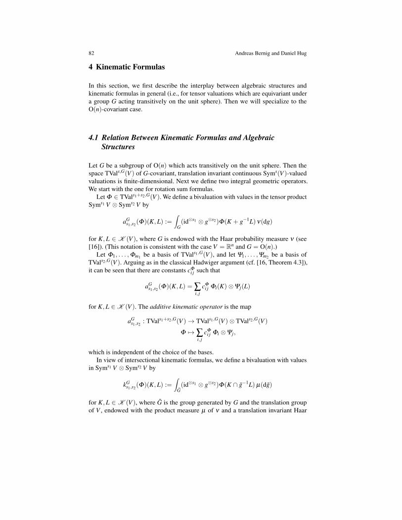
4 Kinematic Formulas

In this section, we first describe the interplay between algebraic structures andkinematic formulas in general (i.e., for tensor valuations which are equivariant undera group G acting transitively on the unit sphere). Then we will specialize to theO(n)-covariant case.

4.1 Relation Between Kinematic Formulas and AlgebraicStructures

Let G be a subgroup of O(n) which acts transitively on the unit sphere. Then thespace TVals,G(V ) of G-covariant, translation invariant continuous Syms(V )-valuedvaluations is finite-dimensional. Next we define two integral geometric operators.We start with the one for rotation sum formulas.

Let Φ ∈ TVals1+s2,G(V ). We define a bivaluation with values in the tensor productSyms1 V ⊗ Syms2 V by

aGs1,s2

(Φ)(K,L) :=∫

G(id⊗s1 ⊗ g⊗s2)Φ(K + g−1L) ν(dg)

for K,L ∈ K (V ), where G is endowed with the Haar probability measure ν (see[16]). (This notation is consistent with the case V = Rn and G = O(n).)

Let Φ1, . . . ,Φm1 be a basis of TVals1,G(V ), and let Ψ1, . . . ,Ψm2 be a basis ofTVals2,G(V ). Arguing as in the classical Hadwiger argument (cf. [16, Theorem 4.3]),it can be seen that there are constants cΦ

i j such that

aGs1,s2

(Φ)(K,L) = ∑i, j

cΦi j Φi(K)⊗Ψj(L)

for K,L ∈ K (V ). The additive kinematic operator is the map

aGs1,s2

: TVals1+s2,G(V )→ TVals1,G(V )⊗ TVals2,G(V )

Φ 7→∑i, j

cΦi j Φi ⊗Ψj,

which is independent of the choice of the bases.In view of intersectional kinematic formulas, we define a bivaluation with values

in Syms1 V ⊗ Syms2 V by

kGs1,s2

(Φ)(K,L) :=∫

G(id⊗s1 ⊗ g⊗s2)Φ(K ∩ g−1L) µ(dg)

for K,L ∈ K (V ), where G is the group generated by G and the translation groupof V , endowed with the product measure µ of ν and a translation invariant Haar


measure on V , and where g is the rotational part of g. (Again this notation is consistentwith the special case where G = Gn is the motion group, G = O(n) and µ is themotion invariant Haar measure with its usual normalization as a ‘product measure’.)Choosing bases and arguing as above, we find

kGs1,s2

(Φ)(K,L) = ∑i, j

dΦi j Φi(K)⊗Ψj(L) (25)

for K,L ∈ K (V ). Of course, the constants dΦi j depend on the chosen bases and on

Φ , but the operator, called intersectional kinematic operator,

kGs1,s2

: TVals1+s2,G(V )→ TVals1,G(V )⊗ TVals2,G(V )

Φ 7→∑i, j

dΦi j Φi ⊗Ψj,

is independent of these choices.In the following, we explain the connection between these operators and then

provide explicit examples.For this we first lift the Poincare duality maps to tensor-valued valuations. Let

V be a Euclidean vector space with scalar product 〈· , ·〉. For s ≤ r we define thecontraction map by

contr : V⊗s ×V⊗r → V⊗(r−s),

(v1 ⊗ . . .⊗ vs,w1 ⊗ . . .⊗ wr) 7→ 〈v1,w1〉〈v2,w2〉 . . . 〈vs,ws〉ws+1 ⊗ · · · ⊗ wr,

and linearity. This map restricts to a map contr : Syms V × Symr V → Symr−s V . Inparticular, if r = s, the map Syms V × Syms V → R is the usual scalar product onSyms V , which will also be denoted by 〈· , ·〉.

The trace map tr : Syms V → Syms−2 V is defined by restriction of the mapV⊗s → V⊗(s−2), v1 ⊗ . . .⊗ vs 7→ 〈v1, v2〉v3 ⊗ . . .⊗ vs, for s ≥ 2.

The scalar product on Syms V induces an isomorphism qs : Syms V → (Syms V )∗

and we set

pdsc : TVals,∞ = Val∞⊗Syms V

pdc ⊗qs

−−−−→ (Val∞)∗ ⊗ (Syms V )∗ = (TVals,∞)∗,

pdsm : TVals,∞ = Val∞⊗Syms V

pdm ⊗qs

−−−−→ (Val∞)∗ ⊗ (Syms V )∗ = (TVals,∞)∗.

From Proposition 2.7 it follows easily that

pdsm = (−1)s pds

c . (26)

Finally, we write

m, c : TVals1,∞(V )⊗ TVals2,∞(V )→ TVals1+s2,∞(V )


for the maps corresponding to the product and the convolution. Moreover, we writemG, cG for the restrictions of these maps to the corresponding spaces of G-covarianttensor valuations.

Theorem 2.10. Let G be a compact subgroup of O(n) acting transitively on the unitsphere. Then the diagram

TVals1+s2,GaG

s1,s2 //

pds1+s2c��

TVals1,G⊗TVals2,G

pds1c ⊗ pd

s2c��(

TVals1+s2,G)∗ c∗G //

F∗��

(TVals1,G

)∗ ⊗ (TVals2,G)∗

F∗⊗F∗��(

TVals1+s2,G)∗ m∗G //

(TVals1,G

)∗ ⊗ (TVals2,G)∗

TVals1+s2,GkG

s1 ,s2 //

pds1+s2m

OO

TVals1,G⊗TVals2,G

pds1m ⊗ pd

s2m

OO

commutes and encodes the relations between product, convolution, Alesker-Fouriertransform, intersectional and additive kinematic formulas.

This diagram allows us to express the additive kinematic operator in terms of theintersectional kinematic operator, and vice versa, with the Fourier transform as thelink between these operators.

Corollary 2.11. Intersectional and additive kinematic formulas are related by theAlesker-Fourier transform in the following way:

aG =(F−1 ⊗ F−1) ◦ kG ◦ F,

or equivalentlykG = (F⊗ F) ◦ aG ◦ F−1.

This follows by looking at the outer square in Theorem 2.10, by carefully takinginto account the signs coming from (26).

4.2 Some Explicit Examples of Kinematic Formulas

We start with a description of a Crofton formula for tensor valuations. Combiningthe connection between Crofton formulas and the product of valuations (see [4, (2)and (16)]) and the explicit formulas for the product of tensor valuations given in (20),we obtain

Integral Geometry and Algebraic Structures for Tensor Valuations 85∫A(n,n−l)

Φsk(K ∩ E) µn−l(dE) =

[nl

]−1 (Φ

sk ·Φ0

l)(K)

=

[nl

]−1(k + lk

)kl

k + l

b s2c

∑a=0,2a 6=s−1

1(4π)aa!

×a

∑m=0

(−1)a−m(

am

)ωs−2m+k+l

ωs−2m+kωlQa

Φs−2ak+l .

After simplification of the inner sum by means of Zeilberger’s algorithm, weobtain the Crofton formula in the Φ-basis which was obtained in [6].

Theorem 2.12. If k, l ≥ 0 with k + l ≤ n and s ∈ N0, then

∫A(n,n−l)

Φsk(K ∩ E) µn−l(dE) =

[nl

]−1(k + lk

)kl

2(k + l)1

Γ( k+l+s

2

)×b s

2 c

∑j=0

Γ( l

2 + j)

Γ( k+s

2 − j)

(4π) j j!Q j

Φs−2 jk+l (K).

The result is also true in the cases k, l ∈ {0, n}, if the right-hand side is interpretedproperly; see the comments after [6, Theorem 3]. The same is true for the next result.

Comparing the trace-free part of this formula (or by inversion), we deduce theCrofton formula for the Ψ -basis, in which the result has a particularly convenientform.

Corollary 2.13. If k, l ≥ 0 and k + l ≤ n, then

∫A(n,n−l)

Ψs

k (K ∩ E) µn−l(dE) =ωs+k+l

ωs+kωl

(k + l

k

)kl

k + l

[nl

]−1

Ψs

k+l(K).

Alternatively, as observed in [10], Corollary 2.13 can be deduced from (12), andthen Theorem 2.12 can be obtained as a consequence.

Thus, having now a convenient Crofton formula for tensor valuations, we deducefrom Hadwiger’s general integral geometric theorem an intersectional kinematicformula in the Ψ -basis.

Theorem 2.14. Let K,M ∈ K n and j ∈ {0, . . . , n}. Then

∫Gn

Ψsj (K ∩ gM) µ(dg) =

n

∑k= j

ωs+k

ωs+ jκk− j

(k − 1j − 1

)[n

k − j

]−1

Ψs

k (K)Vn−k+ j(M).

Let us now prove some more refined intersectional kinematic formulas. In princi-ple, we could also use Corollary 2.11 to find the intersectional kinematic formulasonce we know the additive formulas. The problem is that (15) only gives us the valueof as1,s2 on the basis element φ

s1+s2j , but not on multiples of such basis elements with


powers of the metric tensors. However, such terms appear naturally in the Fouriertransform.

We therefore use Theorem 2.10 with V = Rn and G = O(n), more precisely thelower square in the diagram.

In (20) we have computed the product of two tensor valuations. For fixed (small)ranks s1, s2, the formula simplifies and can be evaluated in a closed form. For instance,if 1 ≤ k, l with k + l ≤ n and s1 = s2 = 3, we get

Φ3k ·Φ3

l =(k + 1)(l + 1)Γ

( k+l+12

)π

52 (k + l + 4)(k + l + 2)(k + l)Γ

( k2

)Γ( l

2

) ··(−32Φ

6k+lπ

3 + 8QΦ4k+lπ

2 − Q2Φ

2k+lπ +

112

Q3Φ

0k+l

). (27)

Let us next work out the vertical arrows in the diagram of Theorem 2.10, that is,the Poincare duality pdm. Again, this is a computation involving differential forms.The result (see [6, Corollary 5.3]) is

〈pdsm(Φ

sk),Φ

sn−k〉 = (−1)s 1− s

πss!2

(nk

)k(n− k)

4Γ( k+s

2

)Γ( n−k+s

2

)Γ( n

2 + 1) . (28)

We now explain how to compute the intersectional kinematic formula kO(n)3,3 with

this knowledge.Since Φ1

m ≡ 0, it is clear that there is a formula of the form

kO(n)3,3 (Φ6

i ) = ∑k+l=n+i

an,i,kΦ3k ⊗Φ

3l

with some constants an,i,k which remain to be determined. Fix k, l with k + l = n + i.Using (28), we find

〈pd3m Φ

3k ,Φ

3n−k〉 =

172π3

(nk

)k(n− k)

Γ( k+3

2

)Γ( n−k+3

2

)Γ( n

2 + 1) ,

〈pd3m Φ

3l ,Φ

3n−l〉 =

172π3

(nl

)l(n− l)

Γ( l+3

2

)Γ( n−l+3

2

)Γ( n

2 + 1) ,

and therefore

〈(pd3m⊗ pd3

m) ◦ kO(n)3,3 (Φ6

i ),Φ3n−k ⊗Φ

3n−l〉

= an,i,k1

72π3

(nk

)k(n− k)

Γ( k+3

2

)Γ( n−k+3

2

)Γ( n

2 + 1)

· 172π3

(nl

)l(n− l)

Γ( l+3

2

)Γ( n−l+3

2

)Γ( n

2 + 1) .


On the other hand, by (27) and (28),

〈m∗O(n) ◦ pd6m(Φ

6i ),Φ

3n−k ⊗Φ

3n−l〉 = 〈pd6

m(Φ6i ),Φ

3n−k ·Φ3

n−l〉

=(n− k + 1)(n− l + 1)Γ

( n−i+12

)π

52 (n− i + 4)(n− i + 2)(n− i)Γ

( n−l2

)Γ( n−k

2

) ··⟨

pd6m(Φ

6i ),−32Φ

6n−iπ

3 + 8QΦ4n−iπ

2 − Q2Φ

2n−iπ +

112

Q3Φ

0n−i

⟩=

1207360

(k − n− 1)(i− k − 1)Γ( n+1

2

)(i + 1)(i− 1)(i− 3)

π5Γ( i+1

2

)Γ( n−k

2

)Γ( k−i

2

) .

From this, the explicit value of an,i,k given in the theorem follows. Comparing theseexpressions, we find that

an,i,k =(i + 1)(i− 1)(i− 3)40Γ

( n+12

)Γ( i+1

2

) Γ( k

2

)Γ( l

2

)(k + 1)(l + 1)

.

We summarize the result in the following theorem.

Theorem 2.15. Let K,M ∈ K n and i ∈ {0, . . . , n− 1}. Then∫Gn

(id⊗3 ⊗ g⊗3)Φ6i (K ∩ g−1M) µ(dg)

=(i + 1)(i− 1)(i− 3)40Γ

( n+12

)Γ( i+1

2

) ∑k+l=n+i

Γ( k

2

)Γ( l

2

)(k + 1)(l + 1)

Φ3k (K)⊗Φ

3l (M).

The same technique can be applied to all bidegrees, but it seems hard to find aclosed formula which is valid simultaneously in all cases.

References

1. Alesker, S., Continuous rotation invariant valuations on convex sets. Ann. of Math. 149 (1999),977–1005.

2. Alesker, S., Description of continuous isometry covariant valuations on convex sets. Geom.Dedicata 74 (1999), 241–248.

3. Alesker, S., Bernig, A., Schuster, F., Harmonic analysis of translation invariant valuations.Geom. Funct. Anal. 21 (2011),751–773.

4. Bernig, A., Algebraic integral geometry. In: Global differential geometry. Springer Proc. Math.17, Springer, Berlin (2012), 107–145. arXiv:1004.3145

5. Bernig, A., Fu., J.H.G., Convolution of convex valuations. Geom. Dedicata, 123 (2006),153–169.

6. Bernig, A., Hug, D., Kinematic formulas for tensor valuations. J. Reine Angew. Math. (toappear), arxiv:1402.2750.

7. Hug, D., Schneider, R., Schuster, R., Integral geometry of tensor valuations. Adv. in Appl.Math., 41 (2008), 482–509.


8. Goodey, P., Weil, W., Sums of sections, surface area measures and the general Minkowskiproblem. J. Diff. Geom. 97 (2014), 477–514.

9. Goodey, P., V. Yaskin, M. Yaskina, Fourier transforms and the Funk-Hecke theorem in convexgeometry. J. Lond. Math. Soc. 80 (2009), 388–404.

10. Goodey, P., Hug, D., Weil, W., Kinematic formulas for area measures. Indiana Univ. Math. J.(to appear), arXiv:1507.03353.

11. McMullen, P., Isometry covariant valuations on convex bodies. Rend. Circ. Mat. Palermo, Ser.II, Suppl. 50 (1997), 259–271.

12. Olafsson, G., Pasquale, A., The Cosλ and Sinλ transforms as intertwining operators betweengeneralized principal series representations of SL(n + 1,K). Adv. Math., 229 (2012), 267–293.

13. Schneider, R., Convex bodies: the Brunn-Minkowski theory, volume 151 of Encyclopedia ofMathematics and its Applications. Cambridge University Press, Cambridge, expanded edition,2014.

14. Schneider, R., Weil, W., Stochastic and Integral Geometry. Probability and Its Applications.Springer, Berlin, 2008.

15. Schuster, F., Wannerer, T., Minkowski Valuations and Generalized Valuations. J. of the EMS(to appear), arXiv:1507.05412.

16. Wannerer, T., Integral geometry of unitary area measures. Adv. Math. 263 (2014), 1–44.17. Weil, W., On surface area measures of convex bodies. Geom. Dedicata 9 (1980), 299–306.

kit - integral geometry and algebraic structures for …hug/media/90.pdfinstitut fur mathematik,...

Documents