KNN-ID and Neural Nets

KNN, ID Trees, and Neural Nets

Intro to Learning Algorithms KNN, Decision trees, Neural Nets are all supervised learning algorithms Their general goal = make accurate predictions about unknown data after being trained on known data. Data comes in form of examples with the general form: x1, .. xn are also known as features, inputs or dimensions y is the output or class label.

Both xi and ys can be discrete (taking on specific values) {0, 1}

or continuous (taking on a range of values) [0, 1] In training we are given (x1, ... xn, y) tuples. In testing (classification), we are given only (x1,...

xn) and the goal is to predict y with high accuracy.

Training error is the classification error measured using training data to test. Testing error is classification error on data not seen in the training phase. K Nearest Neighbors 1-NN

● Given an unknown point, pick the closest 1 neighbor by some distance measure.● Class of unknown is the 1-nearest neighbor's label.

k-NN ● Given an unknown, pick the k closest neighbors by some distance function.● Class of unknown is the mode of the k-nearest neighbor's labels.● k is usually an odd number to facilitate tie breaking.

How to draw 1-NN decision boundaries Decision boundaries, lines on which it is equally likely to be in any of the classes.

1. Examine the region where you think decision boundaries should occur. 2. Find oppositely labeled points (+/-)3. Draw bisectors. (use pencil)4. Extend and join all bisectors. Erase extraneously extended lines.5. Remember to draw boundaries to the edge of the graph and indicate it with arrows! (a very

common mistake).6. Your 1-NN boundaries generally should have sharp edges and corners (otherwise, you are doing

something wrong or drawing boundaries for a higher k-nn.) Distance Functions How to determine what points are "nearest". Here are some standard Distance functions:

Euclidean Distance

Manhattan Distance (Block distance) - Sum of distances in each dimension

Hamming Distance - Sum of differences in each dimension

I(x,y) = 0 if identical, 1 if different.

1

KNN-ID and Neural Nets

Cosine Similarity - Used in Text classification; words are dimensions; documents are vectors of words; vector component is 1 if word i exist.

(Optional) How to Weigh Dimensions Differently In Euclidean distance all dimensions are treated the same. But in practice not dimensions are equally important or useful! For example. Suppose we represent documents as vectors of words. Consider the task of classifying documents related to "Red Sox". If all words are equal, then the word "the" weighs the same as the word "Sox". But almost every english document has the word "the". But only sports related documents have the word "Sox". So we want k-nn distance metrics to weight meaningful words like sox more than functional words like "the". For text classification, a weight scheme used to make some dimensions (words) more important than others is known as: TF-IDF

Here: tf: Words that occur frequently should be weighed more. idf: Words that occur in all the documents (functional-words like the, of etc) should be weighed less. Using this weighing scheme with a distance metric, knn would produce better (more relevant) classifications. Another way to vary the importance of different dimensions is to use: Mahalanobis Distance

Here S is a covariance matrix. Dimensions that show more variance are weighted more.

2

KNN-ID and Neural Nets

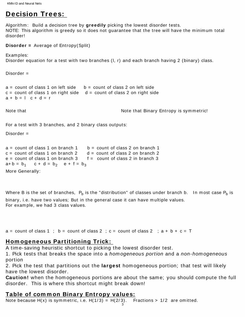
Decision Trees: Algorithm: Build a decision tree by greedily picking the lowest disorder tests.NOTE: This algorithm is greedy so it does not guarantee that the tree will have the minimum total disorder! Disorder = Average of Entropy(Split) Examples: Disorder equation for a test with two branches (l, r) and each branch having 2 (binary) class.

Disorder =

a = count of class 1 on left side b = count of class 2 on left side c = count of class 1 on right side d = count of class 2 on right side a + b = l c + d = r

Note that Note that Binary Entropy is symmetric!

For a test with 3 branches, and 2 binary class outputs:

Disorder =

a = count of class 1 on branch 1 b = count of class 2 on branch 1 c = count of class 1 on branch 2 d = count of class 2 on branch 2 e = count of class 1 on branch 3 f = count of class 2 in branch 3 a+b = b1 c + d = b2 e + f = b3

More Generally:

Where B is the set of branches, Pb is the "distribution" of classes under branch b. In most case Pb is

binary, i.e. have two values; But in the general case it can have multiple values. For example, we had 3 class values.

a = count of class 1 ; b = count of class 2 ; c = count of class 2 ; a + b + c = T Homogeneous Partitioning Trick: A time-saving heuristic shortcut to picking the lowest disorder test. 1. Pick tests that breaks the space into a homogeneous portion and a non-homogeneous portion 2. Pick the test that partitions out the largest homogeneous portion; that test will likely have the lowest disorder. Caution! when the homogeneous portions are about the same; you should compute the full disorder. This is where this shortcut might break down! Table of common Binary Entropy values:Note because H(x) is symmetric, i.e. H(1/3) = H(2/3). Fractions > 1/2 are omitted.

3

KNN-ID and Neural Nets

/3 to /9 /10 to /13

Hnumerator denominator fraction (fraction)

1 3 0.33 0.92

Hnumerator denominator fraction (fraction)

1 10 0.10 0.47

2 3 0.67 0.92 2 10 0.20 0.72

1 4 0.25 0.81 3 10 0.30 0.88

2 4 0.50 1.00 4 10 0.40 0.97

1 5 0.20 0.72 1 11 0.09 0.44

2 5 0.40 0.97 2 11 0.18 0.68

3 5 0.60 0.97 3 11 0.27 0.85

1 6 0.17 0.65 4 11 0.36 0.95

2 6 0.33 0.92 5 11 0.45 0.99

3 6 0.50 1.00 1 12 0.08 0.41

1 7 0.14 0.59 2 12 0.17 0.65

2 7 0.29 0.86 3 12 0.25 0.81

3 7 0.43 0.99 5 12 0.42 0.98

1 8 0.13 0.54 1 13 0.08 0.39

2 8 0.25 0.81 2 13 0.15 0.62

3 8 0.38 0.95 3 13 0.23 0.78

4 8 0.50 1.00 4 13 0.31 0.89

1 9 0.11 0.50 5 13 0.38 0.96

2 9 0.22 0.76 6 13 0.46 1.00

3 9 0.33 0.92

4 9 0.44 0.99

4

KNN-ID and Neural Nets

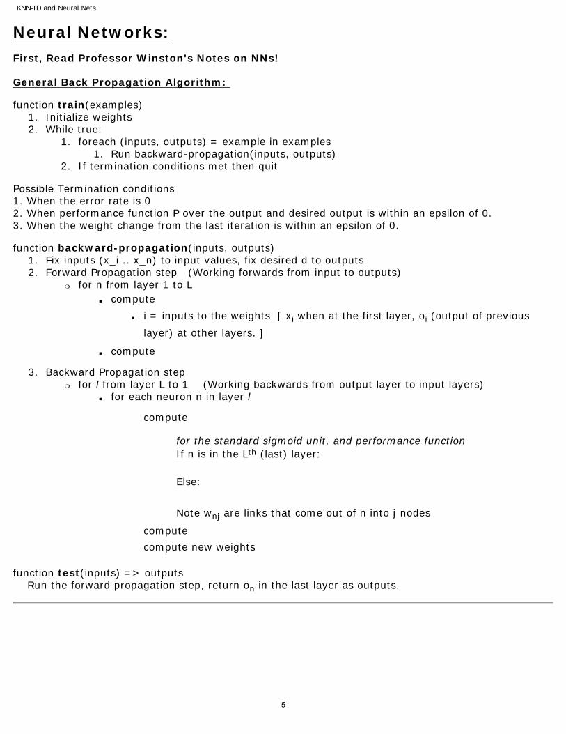
Neural Networks: First, Read Professor Winston's Notes on NNs! General Back Propagation Algorithm: function train(examples)

1. Initialize weights 2. While true:

1. foreach (inputs, outputs) = example in examples1. Run backward-propagation(inputs, outputs)

2. If termination conditions met then quit Possible Termination conditions 1. When the error rate is 0 2. When performance function P over the output and desired output is within an epsilon of 0. 3. When the weight change from the last iteration is within an epsilon of 0. function backward-propagation(inputs, outputs)

1. Fix inputs (x_i .. x_n) to input values, fix desired d to outputs 2. Forward Propagation step (Working forwards from input to outputs)

�❍ for n from layer 1 to L■ compute

■ i = inputs to the weights [ xi when at the first layer, oi (output of previous

layer) at other layers. ]

■ compute

3. Backward Propagation step�❍ for l from layer L to 1 (Working backwards from output layer to input layers)

■ for each neuron n in layer l

compute

for the standard sigmoid unit, and performance function If n is in the Lth (last) layer: Else:

Note wnj are links that come out of n into j nodes

compute

compute new weights function test(inputs) => outputs Run the forward propagation step, return on in the last layer as outputs.

5

KNN-ID and Neural Nets

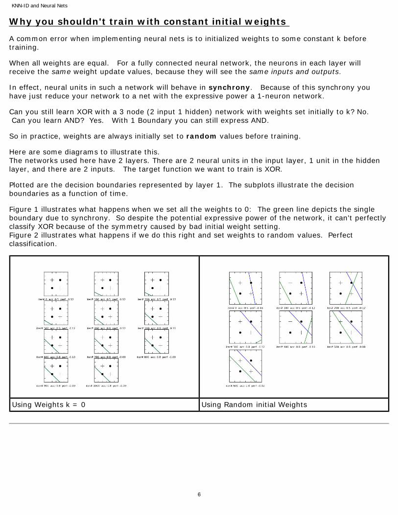
Using Weights k = 0 Using Random initial Weights

Why you shouldn't train with constant initial weights A common error when implementing neural nets is to initialized weights to some constant k before training. When all weights are equal. For a fully connected neural network, the neurons in each layer will receive the same weight update values, because they will see the same inputs and outputs. In effect, neural units in such a network will behave in synchrony. Because of this synchrony you have just reduce your network to a net with the expressive power a 1-neuron network. Can you still learn XOR with a 3 node (2 input 1 hidden) network with weights set initially to k? No. Can you learn AND? Yes. With 1 Boundary you can still express AND. So in practice, weights are always initially set to random values before training. Here are some diagrams to illustrate this. The networks used here have 2 layers. There are 2 neural units in the input layer, 1 unit in the hidden layer, and there are 2 inputs. The target function we want to train is XOR. Plotted are the decision boundaries represented by layer 1. The subplots illustrate the decision boundaries as a function of time. Figure 1 illustrates what happens when we set all the weights to 0: The green line depicts the single boundary due to synchrony. So despite the potential expressive power of the network, it can't perfectly classify XOR because of the symmetry caused by bad initial weight setting. Figure 2 illustrates what happens if we do this right and set weights to random values. Perfect classification.

6

KNN-ID and Neural Nets

A B T WA WB WT z o d d-o

forward 0 0 -1 0 0 1 a) -1 b) 0.27 1 (1-0.27) =0.73

backward

forward

0

1

-1

c) 0

0

d) 0

0

e) 0.86

0.86

f) -0.86

g) 0.30

1

(1-0.3) = 0.7

backward

forward

1

0

-1

h) 0

0

i) 0.15

0.15

j) 0.71

0.71

k) -0.71

l) 0.33

0

(0-0.33) =-0.33

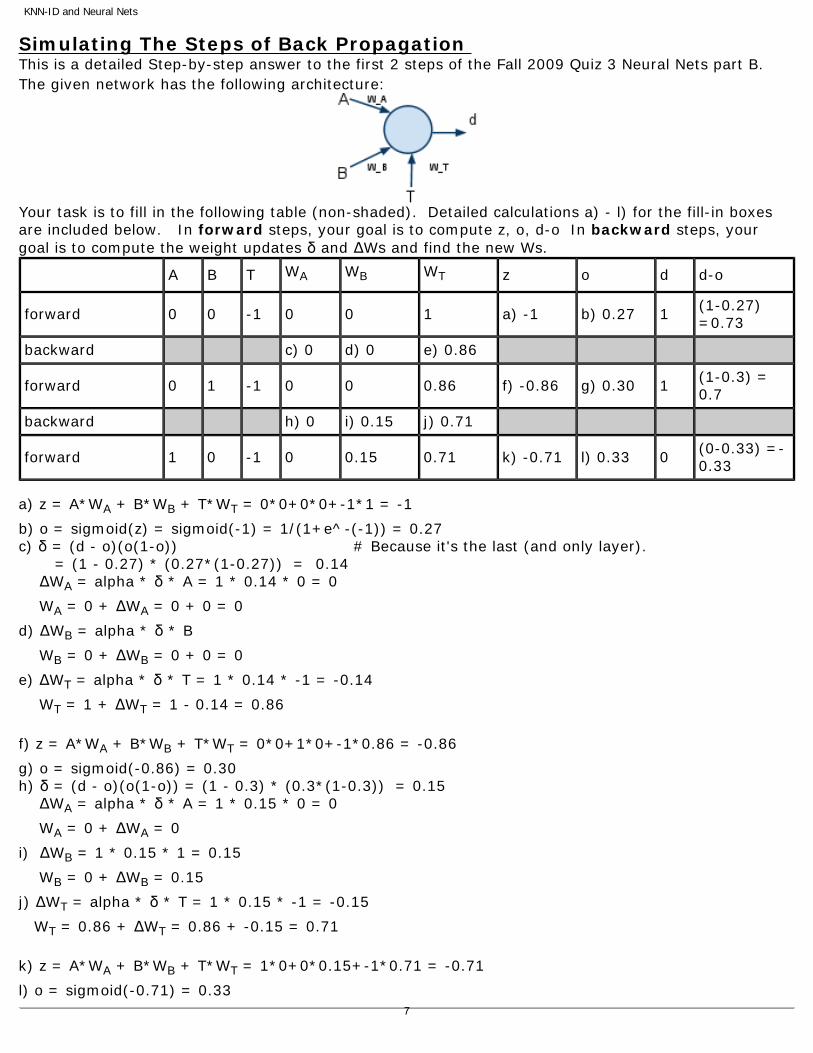
Simulating The Steps of Back Propagation This is a detailed Step-by-step answer to the first 2 steps of the Fall 2009 Quiz 3 Neural Nets part B. The given network has the following architecture:

Your task is to fill in the following table (non-shaded). Detailed calculations a) - l) for the fill-in boxes are included below. In forward steps, your goal is to compute z, o, d-o In backward steps, your goal is to compute the weight updates δ and ΔWs and find the new Ws.

a) z = A*WA + B*WB + T*WT = 0*0+0*0+-1*1 = -1

b) o = sigmoid(z) = sigmoid(-1) = 1/(1+e^-(-1)) = 0.27 c) δ = (d - o)(o(1-o)) # Because it's the last (and only layer). = (1 - 0.27) * (0.27*(1-0.27)) = 0.14 ΔWA = alpha * δ * A = 1 * 0.14 * 0 = 0

WA = 0 + ΔWA = 0 + 0 = 0

d) ΔWB = alpha * δ * B

WB = 0 + ΔWB = 0 + 0 = 0

e) ΔWT = alpha * δ * T = 1 * 0.14 * -1 = -0.14

WT = 1 + ΔWT = 1 - 0.14 = 0.86

f) z = A*WA + B*WB + T*WT = 0*0+1*0+-1*0.86 = -0.86

g) o = sigmoid(-0.86) = 0.30 h) δ = (d - o)(o(1-o)) = (1 - 0.3) * (0.3*(1-0.3)) = 0.15 ΔWA = alpha * δ * A = 1 * 0.15 * 0 = 0

WA = 0 + ΔWA = 0

i) ΔWB = 1 * 0.15 * 1 = 0.15

WB = 0 + ΔWB = 0.15

j) ΔWT = alpha * δ * T = 1 * 0.15 * -1 = -0.15

WT = 0.86 + ΔWT = 0.86 + -0.15 = 0.71

k) z = A*WA + B*WB + T*WT = 1*0+0*0.15+-1*0.71 = -0.71

l) o = sigmoid(-0.71) = 0.33 7

KNN-ID and Neural Nets

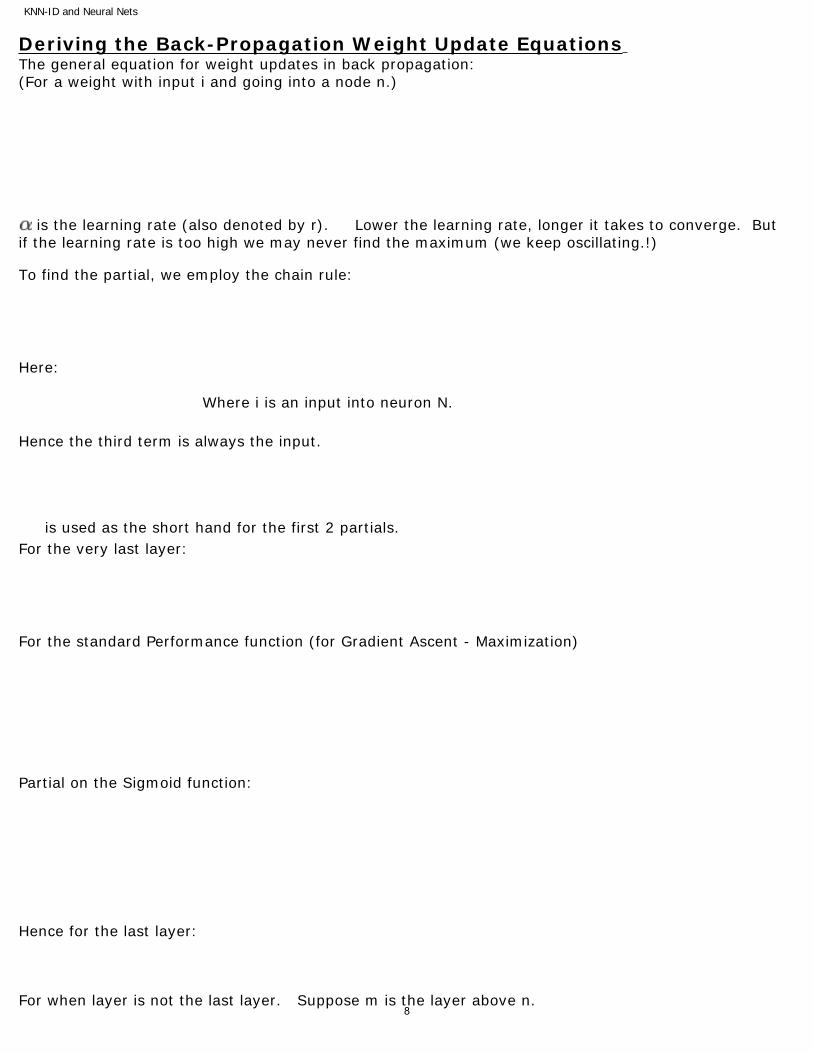
Deriving the Back-Propagation Weight Update Equations The general equation for weight updates in back propagation: (For a weight with input i and going into a node n.)

is the learning rate (also denoted by r). Lower the learning rate, longer it takes to converge. But

if the learning rate is too high we may never find the maximum (we keep oscillating.!) To find the partial, we employ the chain rule:

Here: Where i is an input into neuron N.

Hence the third term is always the input.

is used as the short hand for the first 2 partials.

For the very last layer:

For the standard Performance function (for Gradient Ascent - Maximization)

Partial on the Sigmoid function:

Hence for the last layer: For when layer is not the last layer. Suppose m is the layer above n.

8

KNN-ID and Neural Nets

= =

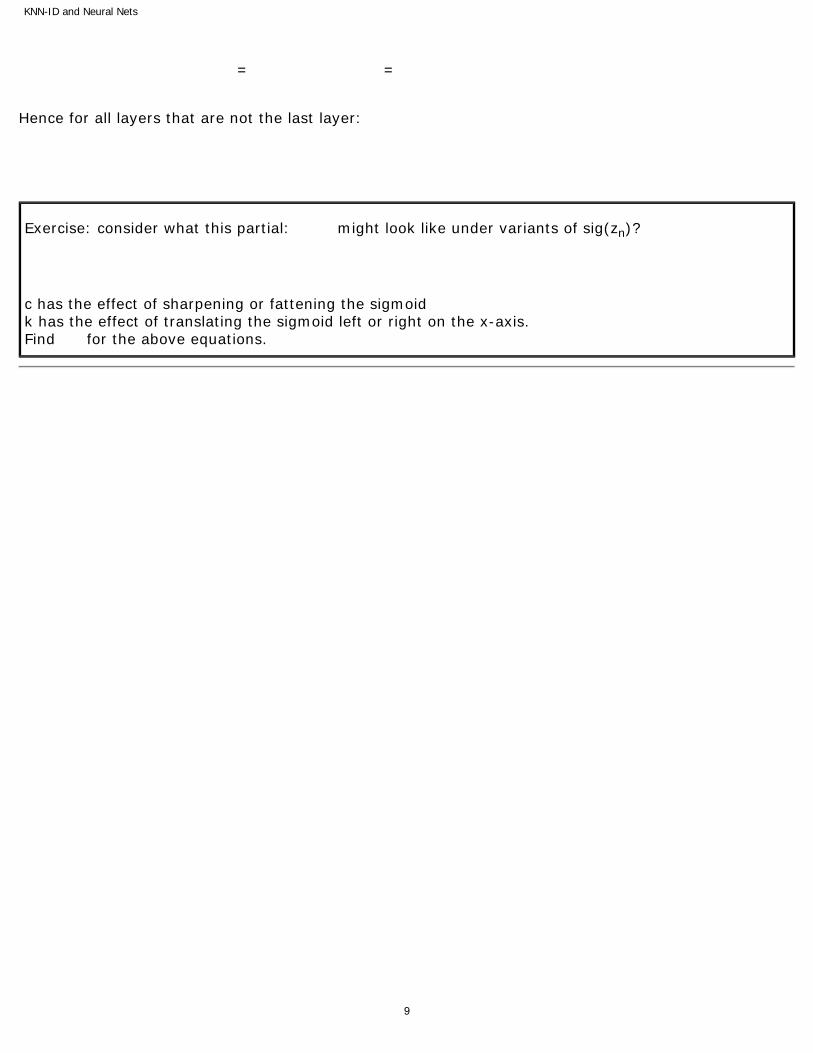
Hence for all layers that are not the last layer:

Exercise: consider what this partial: might look like under variants of sig(zn)?

c has the effect of sharpening or fattening the sigmoid k has the effect of translating the sigmoid left or right on the x-axis. Find for the above equations.

9

KNN-ID and Neural Nets

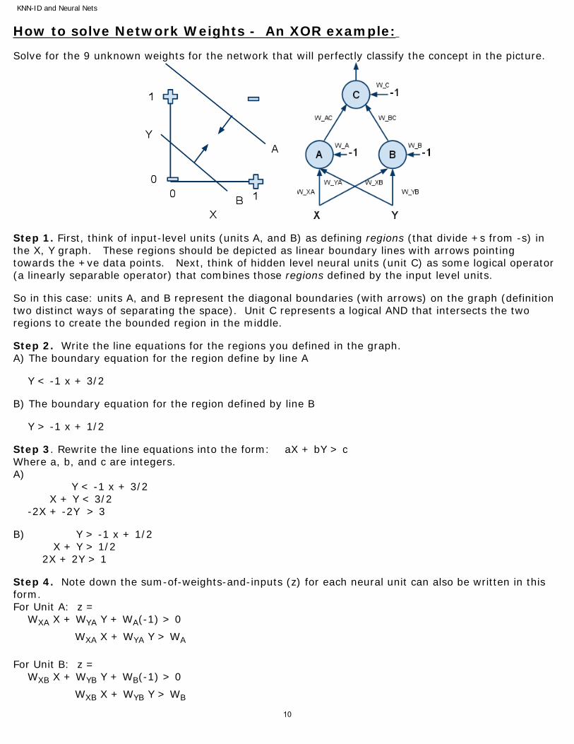
How to solve Network Weights - An XOR example: Solve for the 9 unknown weights for the network that will perfectly classify the concept in the picture.

Step 1. First, think of input-level units (units A, and B) as defining regions (that divide +s from -s) in the X, Y graph. These regions should be depicted as linear boundary lines with arrows pointing towards the +ve data points. Next, think of hidden level neural units (unit C) as some logical operator (a linearly separable operator) that combines those regions defined by the input level units. So in this case: units A, and B represent the diagonal boundaries (with arrows) on the graph (definition two distinct ways of separating the space). Unit C represents a logical AND that intersects the two regions to create the bounded region in the middle. Step 2. Write the line equations for the regions you defined in the graph. A) The boundary equation for the region define by line A Y < -1 x + 3/2 B) The boundary equation for the region defined by line B Y > -1 x + 1/2 Step 3. Rewrite the line equations into the form: aX + bY > c Where a, b, and c are integers. A) Y < -1 x + 3/2 X + Y < 3/2 -2X + -2Y > 3 B) Y > -1 x + 1/2 X + Y > 1/2 2X + 2Y > 1 Step 4. Note down the sum-of-weights-and-inputs (z) for each neural unit can also be written in this form. For Unit A: z = WXA X + WYA Y + WA(-1) > 0

WXA X + WYA Y > WA

For Unit B: z = WXB X + WYB Y + WB(-1) > 0

WXB X + WYB Y > WB

10

KNN-ID and Neural Nets

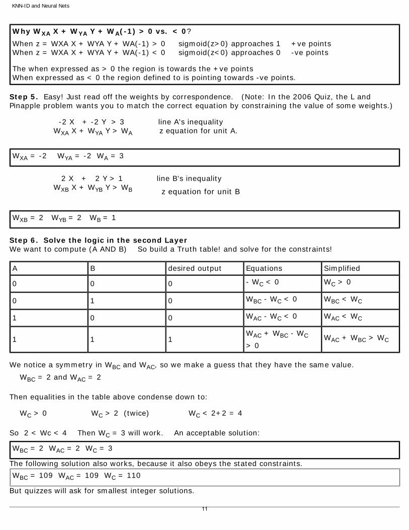
A B desired output Equations Simplified

0 0 0 - WC < 0 WC > 0

0 1 0 WBC - WC < 0 WBC < WC

1 0 0 WAC - WC < 0 WAC < WC

1 1 1 WAC + WBC - WC

> 0 WAC + WBC > WC

Why WXA X + WYA Y + WA(-1) > 0 vs. < 0?

When z = WXA X + WYA Y + WA(-1) > 0 sigmoid(z>0) approaches 1 +ve points When z = WXA X + WYA Y + WA(-1) < 0 sigmoid(z<0) approaches 0 -ve points The when expressed as > 0 the region is towards the +ve points When expressed as < 0 the region defined to is pointing towards -ve points.

Step 5. Easy! Just read off the weights by correspondence. (Note: In the 2006 Quiz, the L and Pinapple problem wants you to match the correct equation by constraining the value of some weights.) -2 X + -2 Y > 3 line A's inequality WXA X + WYA Y > WA z equation for unit A.

WXA = -2 WYA = -2 WA = 3

2 X + 2 Y > 1 line B's inequality WXB X + WYB Y > WB z equation for unit B

WXB = 2 WYB = 2 WB = 1

Step 6. Solve the logic in the second Layer We want to compute (A AND B) So build a Truth table! and solve for the constraints!

We notice a symmetry in WBC and WAC, so we make a guess that they have the same value.

WBC = 2 and WAC = 2

Then equalities in the table above condense down to: WC > 0 WC > 2 (twice) WC < 2+2 = 4

So 2 < Wc < 4 Then WC = 3 will work. An acceptable solution:

WBC = 2 WAC = 2 WC = 3

The following solution also works, because it also obeys the stated constraints.

WBC = 109 WAC = 109 WC = 110

But quizzes will ask for smallest integer solutions.

11

KNN-ID and Neural Nets

Overfitting and Underfitting Overfitting

● Occurs when learned model describes randomness or noise instead of the underlying relationship.

● Occurs when a model is excessively complex.● Analogy - "trying to fit a straight line (with noise) using a curve" ● An overfit model will generally have poor predictive performance (high test error). But low

training error. ● It can exaggerate minor fluctuations in the data.

Examples

KNN - Using a low k setting (k=1) to perfectly classify all the data points. But not being aware that some data points are random or due to noise. Using small k makes the model less constrained, and hence the resulting decision boundaries can become very complex. (almost more than necessary).

Decision Tree - Building a really complex tree so that all data points are perfectly classified. While the underlying data has noise or randomness.

Neural Nets - Using a complex multi-layer neural net to classify the (AND function + noise). The network will end up learning the noise as well as the AND function.

Underfitting

● Occurs when a model is too simple, does not capture the true underlying complexity of the data. Also known as bias error.

● Analogy: "trying to fit a curve using a straight line"● An underfit model will generally have poor predictive performance (high test error). Because

it is not sufficiently complex enough to capture all the true structure in the underlying data. Examples

KNN - Using k = total number of data points. This will classify everything as the most frequent class (the mode).

Decision Tree - Using 1 test stump to classify an AND relationship; when one needs a decision tree of at least 2 stumps.

Neural Nets - Using a 1-neuron net to classify an XOR How to Avoid Overfitting / Underfitting Use Cross Validation! N-Fold Cross-validation: Divide the training data into n partitions Join n-1 partitions into a "training set", use the nth partition as the unknowns (test set) Repeat this for n times, and compute the average error or accuracy. Leave-One-Out Cross-validation: A specific case of N-fold. If dataset has N data points, then put N-1 data points in the training set. Use the left-out data point as test. Repeat N times. How to pick a good model:

12

KNN-ID and Neural Nets

Try different models. Pick the model that gives you the lowest CV error. Examples: KNN - vary k from 1 to N-1. Run cross-validation under different ks.Choose the k with the lowest CV error. Decision Tree - Try trees of varying depth, and varying number of tests. Run cross-validation to pick the tree of lowest CV Error. Neural Net - Try different Neural Net architectures. Run CV to pick the architecture of lowest CV Error. Models chosen using cross-validation can generalize better, and are less likely to overfit or underfit.

13

MIT OpenCourseWarehttp://ocw.mit.edu

6.034 Artificial IntelligenceFall 2010

For information about citing these materials or our Terms of Use, visit: http://ocw.mit.edu/terms.