neural networks simple neural nets for pattern classification chapter 2
TRANSCRIPT
Neural Networks
Simple Neural NetsFor Pattern
Classification
CHAPTER 2
Neural Networks2: Simple NN for Pattern Classification 2
General Discussion One of the simplest tasks that neural nets can be
trained to perform is pattern classification. In pattern classification problems, each input vector
(pattern) belongs, or does not belong, to a particular class or category.
For a neural net approach, we assume we have a set of training patterns for which the correct classification is known.
The output unit represents membership in the class with a response of 1; a response of - 1 (or 0 if binary representation is used) indicates that the pattern is not a member of the class.
Neural Networks2: Simple NN for Pattern Classification 3
General Discussion In 1963, neural networks was used to detect heart
abnormalities with EKG types of data as input (46 measurements) and classified them into "normal" or "abnormal”.
When patterns may or may not belong to several classes, there is an output unit for each class.
In this chapter, we shall discuss three methods of training a simple single layer neural net for pattern classification: the Hebb rule, the perceptron learning rule, and the delta rule.
Neural Networks2: Simple NN for Pattern Classification 4
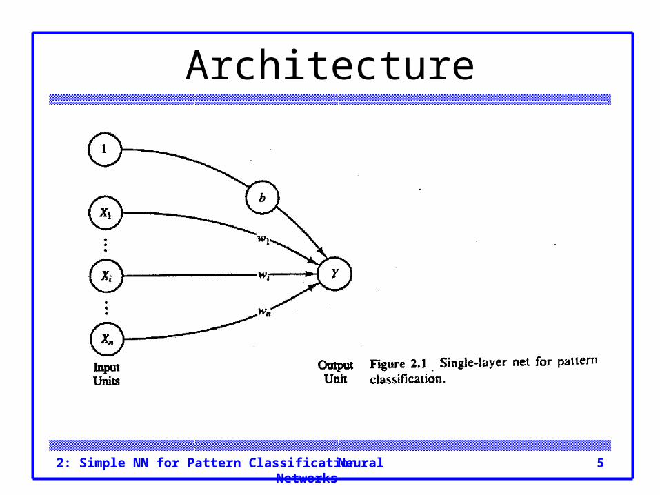
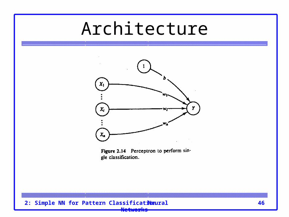
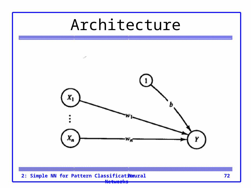
Architecture The basic architecture of the simplest possible
neural networks that perform pattern classification consists of a layer of input units (as many units as the patterns to be classified have components) and a single output unit.
Neural Networks2: Simple NN for Pattern Classification 5
Architecture
Neural Networks2: Simple NN for Pattern Classification 6
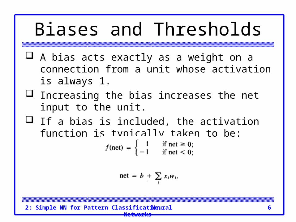
Biases and Thresholds A bias acts exactly as a weight on a connection from
a unit whose activation is always 1. Increasing the bias increases the net input to the
unit. If a bias is included, the activation function is
typically taken to be:
Neural Networks2: Simple NN for Pattern Classification 7
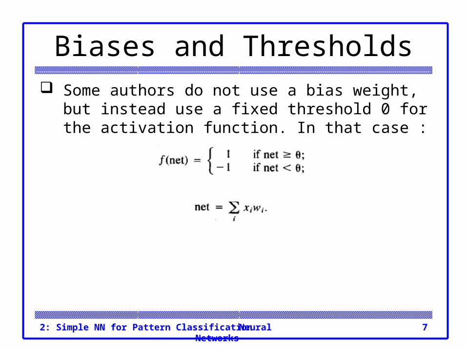
Biases and Thresholds Some authors do not use a bias weight, but instead
use a fixed threshold 0 for the activation function. In that case :
Neural Networks2: Simple NN for Pattern Classification 8
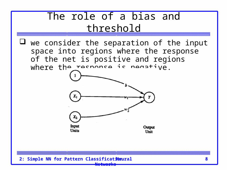
The role of a bias and threshold
we consider the separation of the input space into regions where the response of the net is positive and regions where the response is negative.
Neural Networks2: Simple NN for Pattern Classification 9
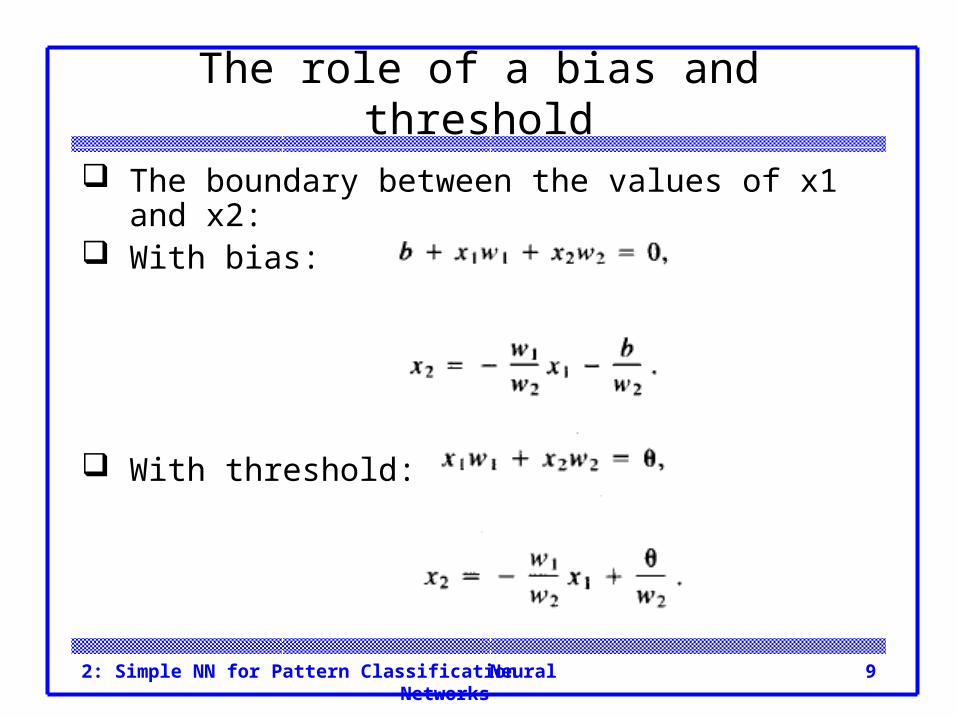
The role of a bias and threshold
The boundary between the values of x1 and x2: With bias:
With threshold:

Neural Networks2: Simple NN for Pattern Classification 10
The role of a bias and threshold
During training, values of w, and w2 are determined so that the net will have the correct response for the training data.
including neither a bias nor a threshold is equivalent to requiring the separating line (or plane or hyperplane for inputs with more components) to pass through the origin.
Neural Networks2: Simple NN for Pattern Classification 11
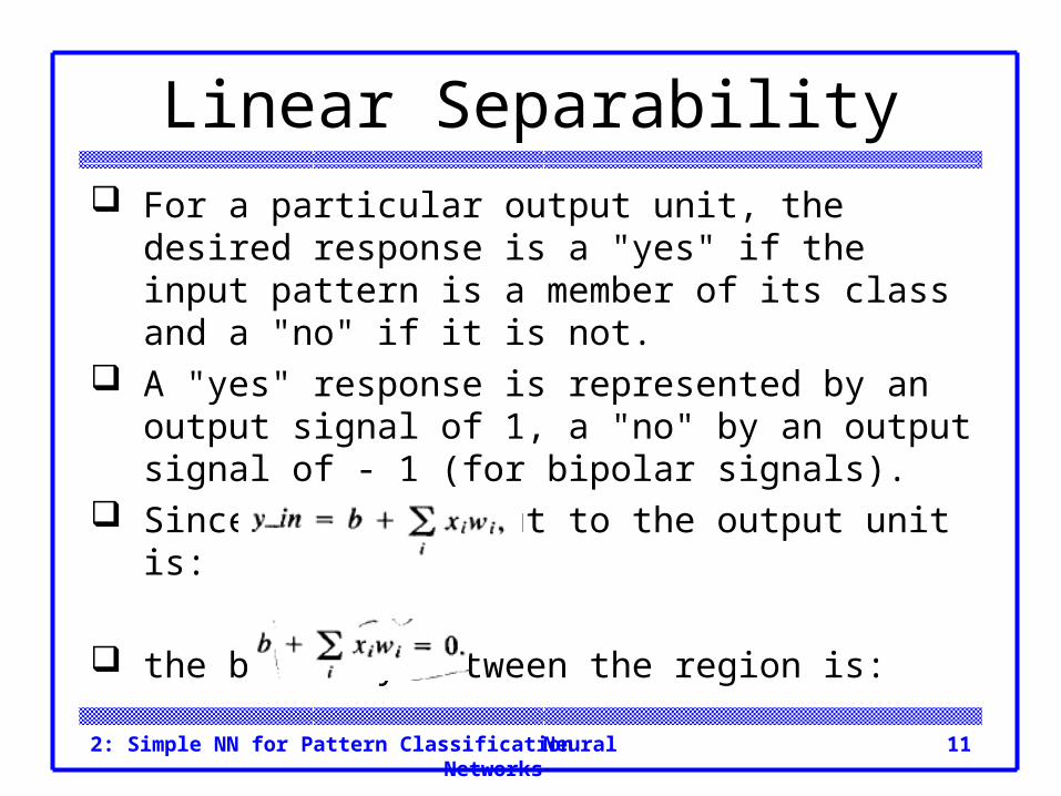
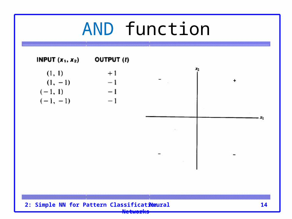
Linear Separability For a particular output unit, the desired response is a
"yes" if the input pattern is a member of its class and a "no" if it is not.
A "yes" response is represented by an output signal of 1, a "no" by an output signal of - 1 (for bipolar signals).
Since the net input to the output unit is:
the boundary between the region is:
Neural Networks2: Simple NN for Pattern Classification 12
Linear Separability If there are weights (and a bias) so that all of the
training input vectors for which the correct response is +1 lie on one side of the decision boundary and all of the training input vectors for which the correct response is -1 lie on the other side of the decision boundary, we say that the problem is "linearly separable."
Neural Networks2: Simple NN for Pattern Classification 13
Linear Separability Minsky and Papert [I988] showed that a single-layer
net can learn only linearly separable problems. Furthermore, it is easy to extend this result to show
that multilayer nets with linear activation functions are no more powerful than single-layer nets (since the composition of linear functions is linear).
Neural Networks2: Simple NN for Pattern Classification 14
AND function
Neural Networks2: Simple NN for Pattern Classification 15
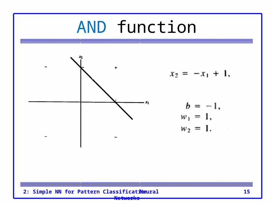
AND function
Neural Networks2: Simple NN for Pattern Classification 16
Linear Separability OR function is also similar to AND function. The equations of the decision boundaries are not
unique. Note that if a bias weight were not included in these
examples, the decision boundary would be forced to go through the origin.
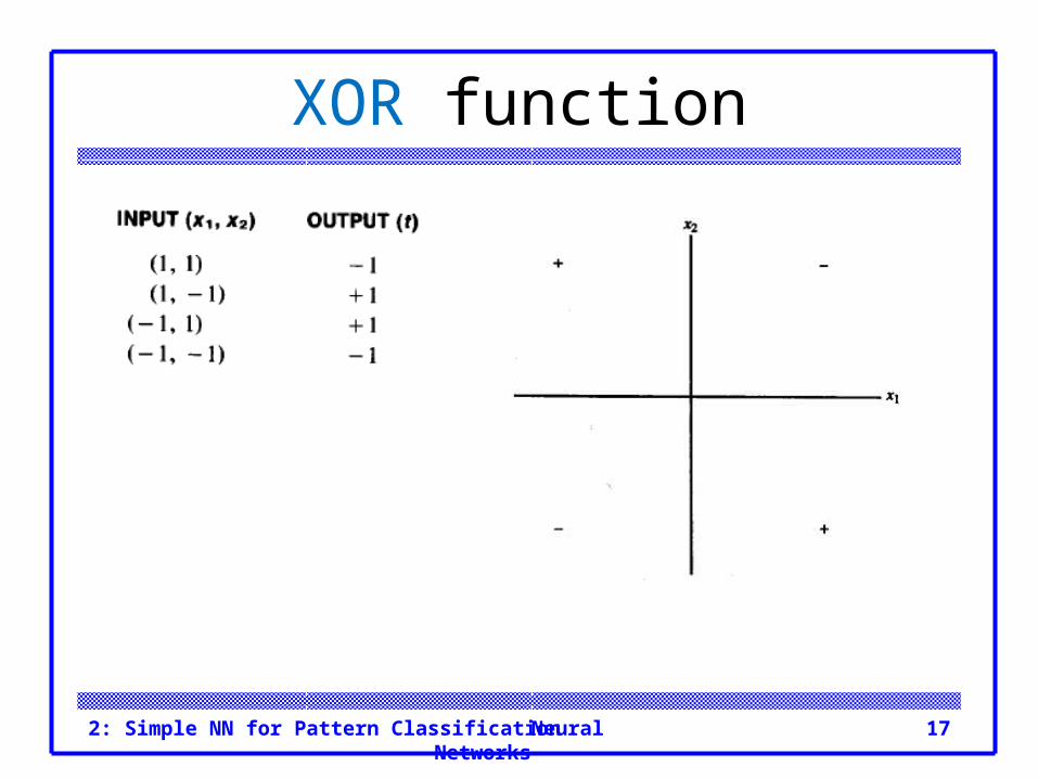
Not all simple two-input, single-output mappings can be solved by a single layer net (even with a bias included), as is illustrated in Example 2.4.
Neural Networks2: Simple NN for Pattern Classification 17
XOR function
Neural Networks2: Simple NN for Pattern Classification 18
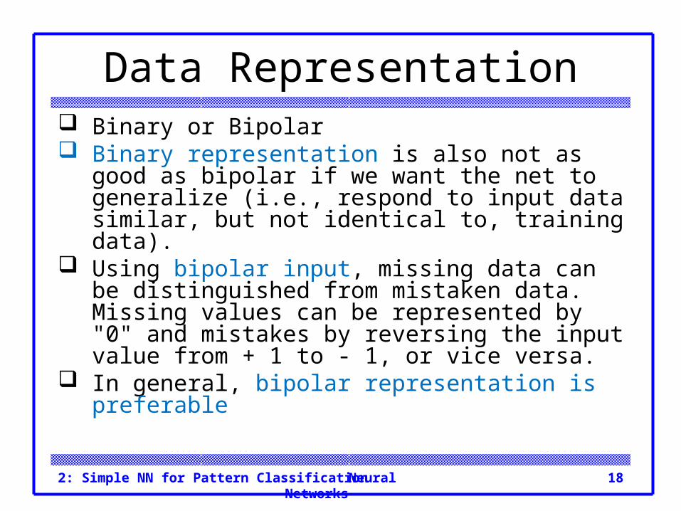
Data Representation Binary or Bipolar Binary representation is also not as good as bipolar
if we want the net to generalize (i.e., respond to input data similar, but not identical to, training data).
Using bipolar input, missing data can be distinguished from mistaken data. Missing values can be represented by "0" and mistakes by reversing the input value from + 1 to - 1, or vice versa.
In general, bipolar representation is preferable
Neural Networks2: Simple NN for Pattern Classification 19
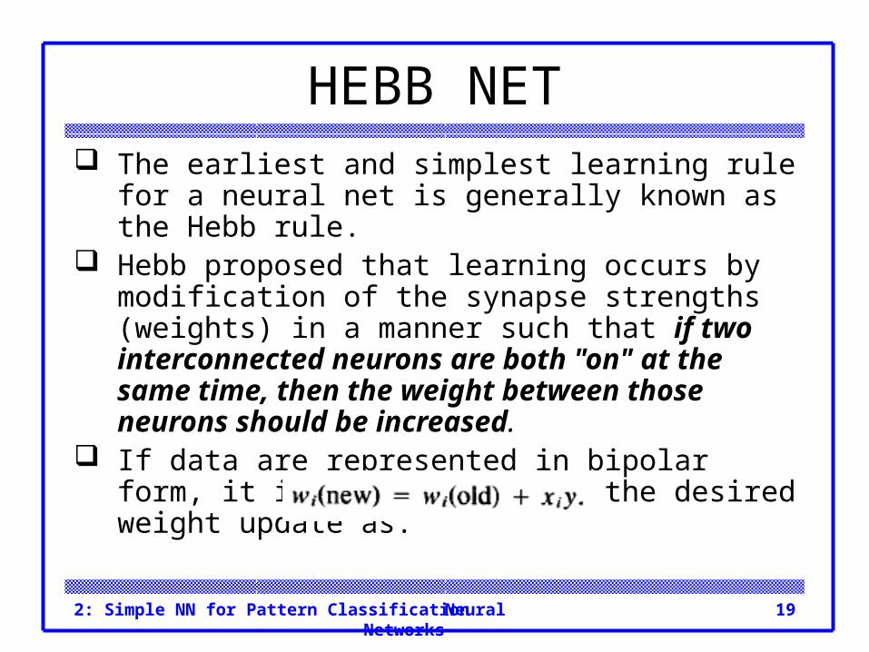
HEBB NET The earliest and simplest learning rule for a neural
net is generally known as the Hebb rule. Hebb proposed that learning occurs by modification
of the synapse strengths (weights) in a manner such that if two interconnected neurons are both "on" at the same time, then the weight between those neurons should be increased.
If data are represented in bipolar form, it is easy to express the desired weight update as:
Neural Networks2: Simple NN for Pattern Classification 20
HEBB NET If the data are binary, this formula does not
distinguish between a training pair in which an input unit is "on" and the target value is "off" and a training pair in which both the input unit and the target value are "off."
Neural Networks2: Simple NN for Pattern Classification 21
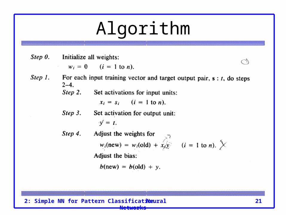
Algorithm
Neural Networks2: Simple NN for Pattern Classification 22
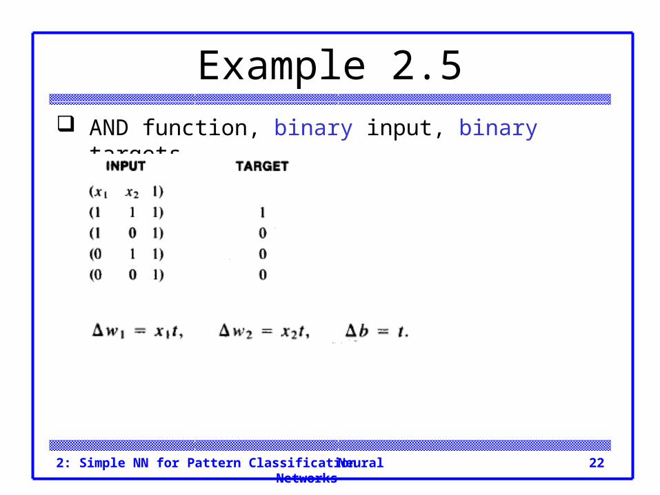
Example 2.5 AND function, binary input, binary targets

Neural Networks2: Simple NN for Pattern Classification 23
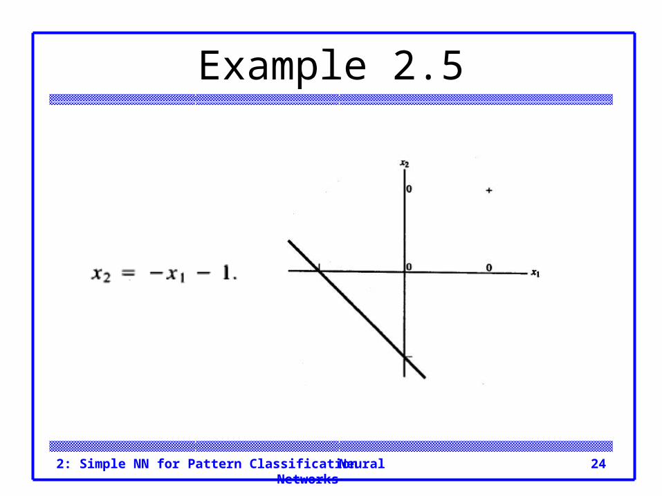
Example 2.5
Neural Networks2: Simple NN for Pattern Classification 24
Example 2.5
Neural Networks2: Simple NN for Pattern Classification 25
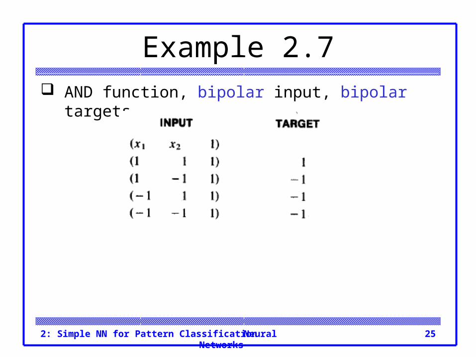
Example 2.7 AND function, bipolar input, bipolar targets
Neural Networks2: Simple NN for Pattern Classification 26
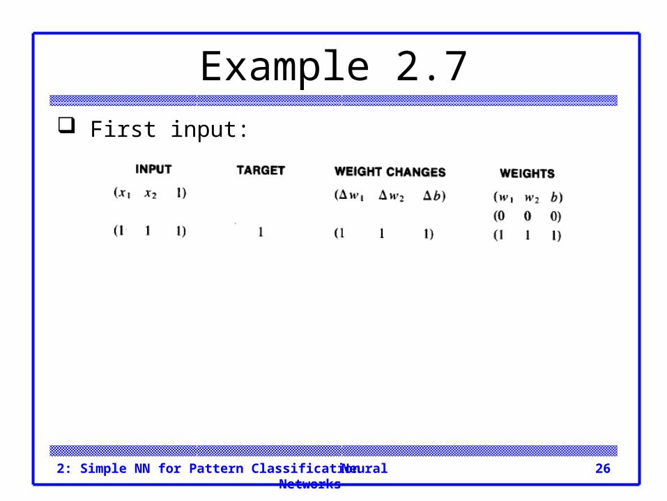
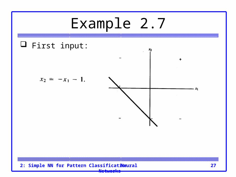
Example 2.7 First input:
Neural Networks2: Simple NN for Pattern Classification 27
Example 2.7 First input:
Neural Networks2: Simple NN for Pattern Classification 28
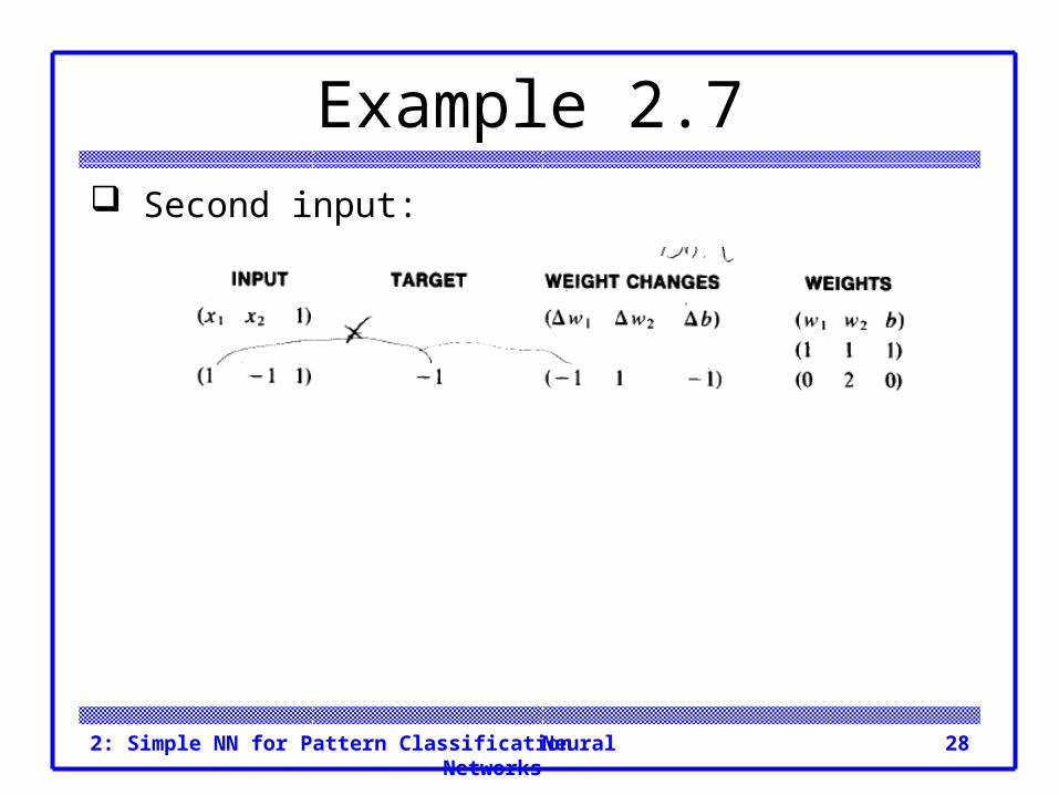
Example 2.7 Second input:

Neural Networks2: Simple NN for Pattern Classification 29
Example 2.7 Second input:
Neural Networks2: Simple NN for Pattern Classification 30
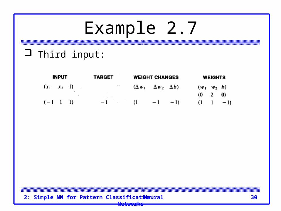
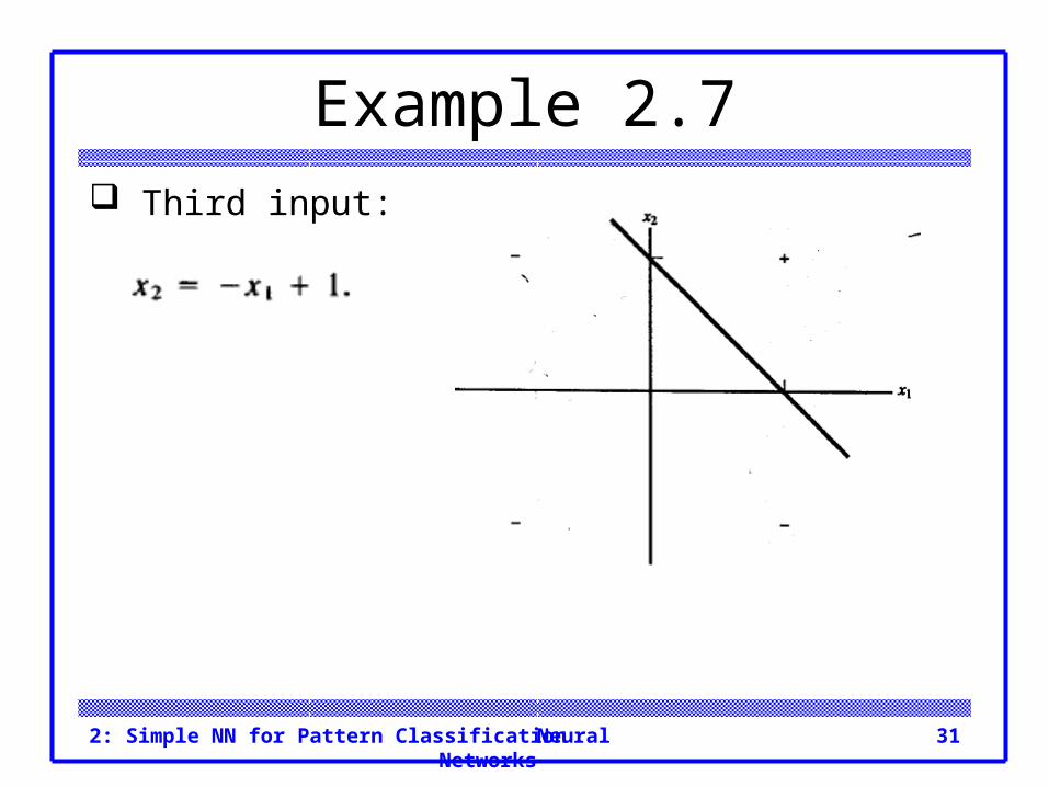
Example 2.7 Third input:
Neural Networks2: Simple NN for Pattern Classification 31
Example 2.7 Third input:
Neural Networks2: Simple NN for Pattern Classification 32
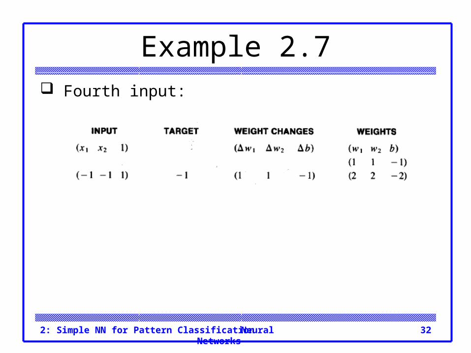
Example 2.7 Fourth input:
Neural Networks2: Simple NN for Pattern Classification 33
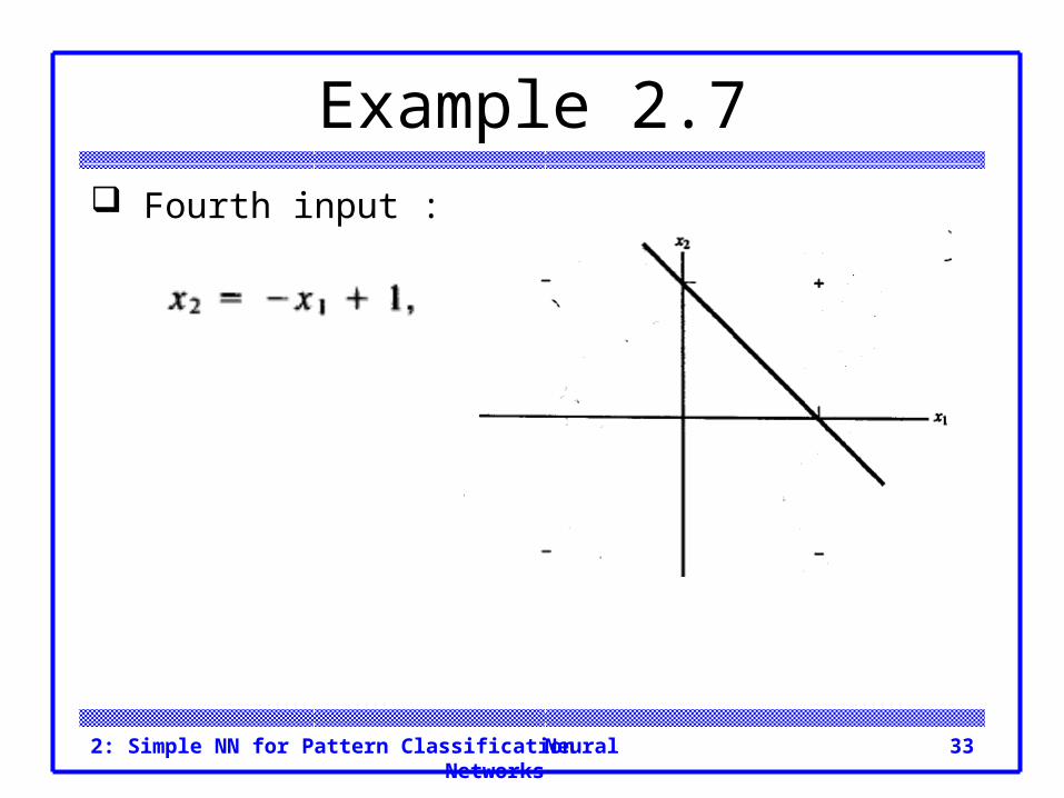
Example 2.7 Fourth input :
Neural Networks2: Simple NN for Pattern Classification 34
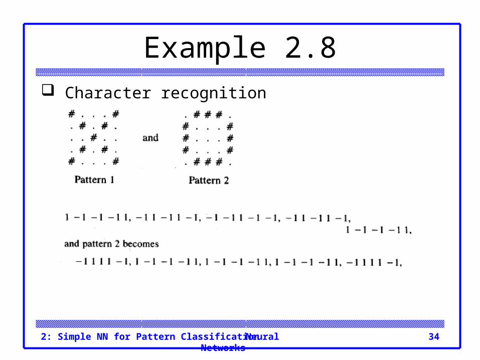
Example 2.8 Character recognition
Neural Networks2: Simple NN for Pattern Classification 35
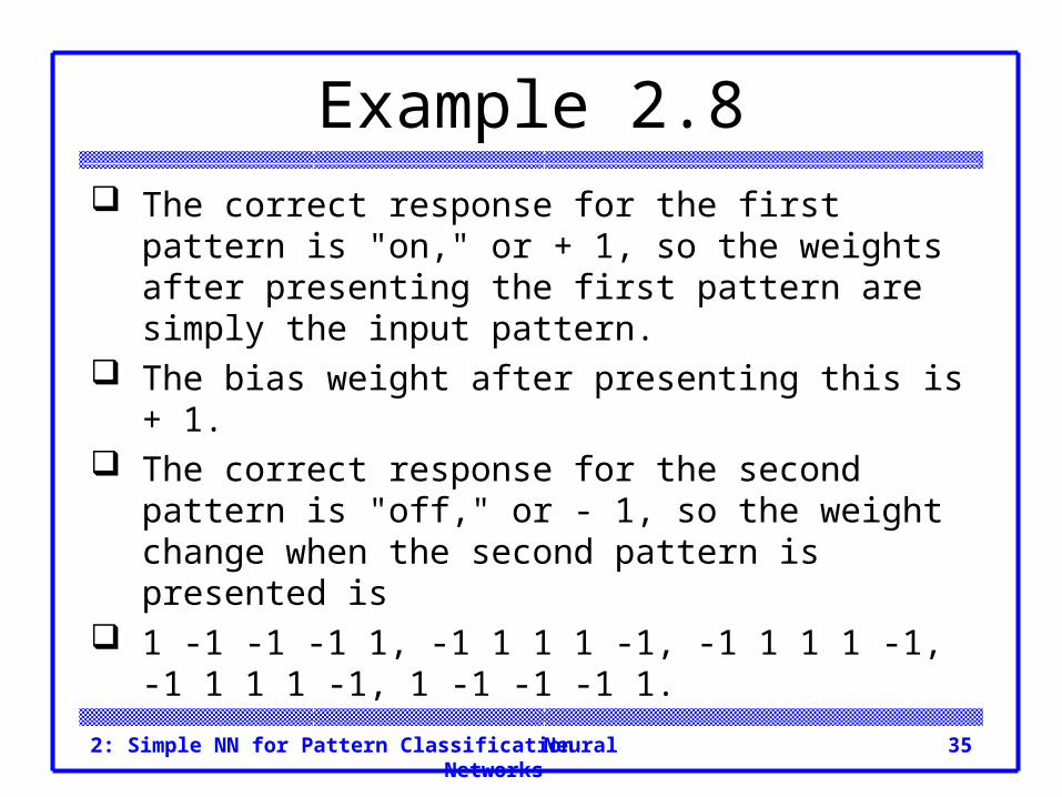
Example 2.8 The correct response for the first pattern is "on," or +
1, so the weights after presenting the first pattern are simply the input pattern.
The bias weight after presenting this is + 1. The correct response for the second pattern is "off,"
or - 1, so the weight change when the second pattern is presented is
1 -1 -1 -1 1, -1 1 1 1 -1, -1 1 1 1 -1, -1 1 1 1 -1, 1 -1 -1 -1 1.
Neural Networks2: Simple NN for Pattern Classification 36
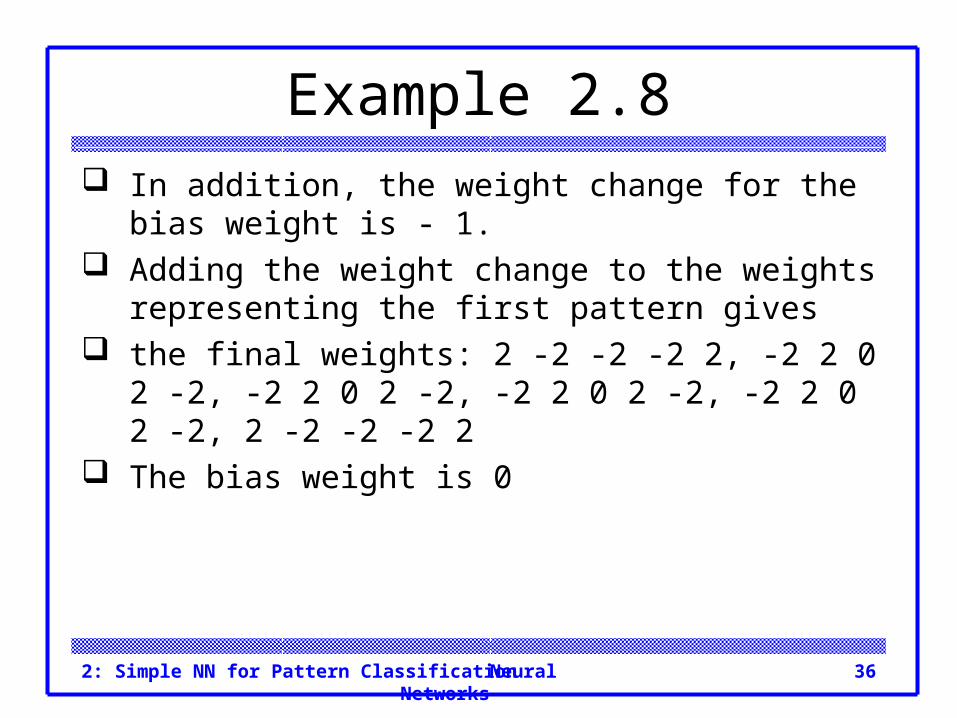
Example 2.8 In addition, the weight change for the bias weight is -
1. Adding the weight change to the weights
representing the first pattern gives the final weights: 2 -2 -2 -2 2, -2 2 0 2 -2, -2 2 0 2 -2,
-2 2 0 2 -2, -2 2 0 2 -2, 2 -2 -2 -2 2 The bias weight is 0
Neural Networks2: Simple NN for Pattern Classification 37
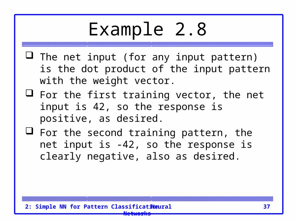
Example 2.8 The net input (for any input pattern) is the dot
product of the input pattern with the weight vector. For the first training vector, the net input is 42, so the
response is positive, as desired. For the second training pattern, the net input is -42,
so the response is clearly negative, also as desired.
Neural Networks2: Simple NN for Pattern Classification 38
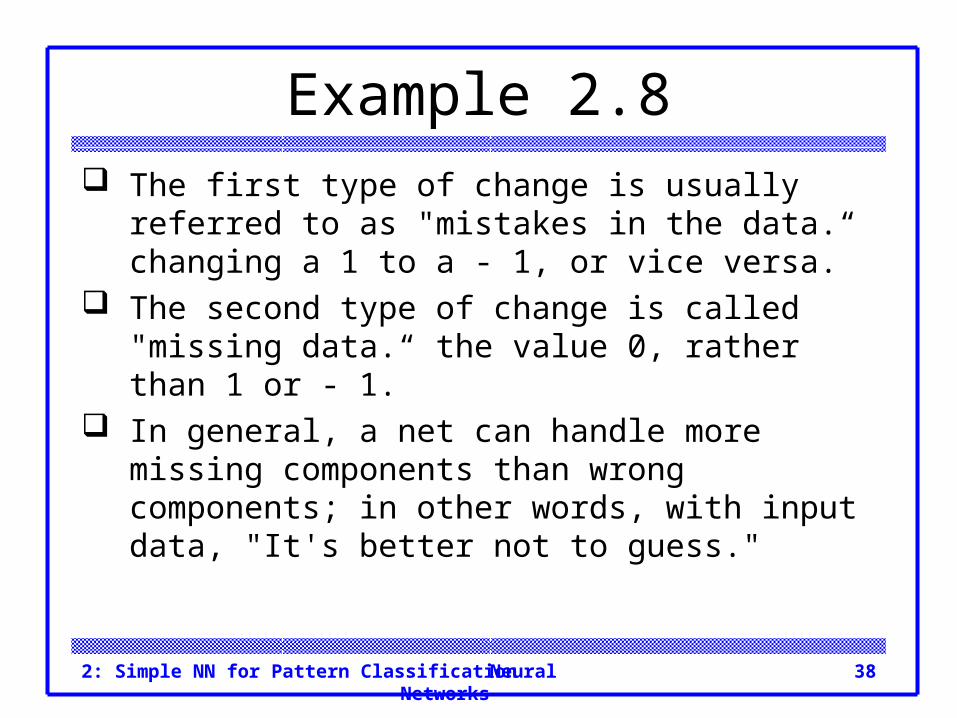
Example 2.8 The first type of change is usually referred to as
"mistakes in the data.“ changing a 1 to a - 1, or vice versa.
The second type of change is called "missing data.“ the value 0, rather than 1 or - 1.
In general, a net can handle more missing components than wrong components; in other words, with input data, "It's better not to guess."
Neural Networks2: Simple NN for Pattern Classification 39
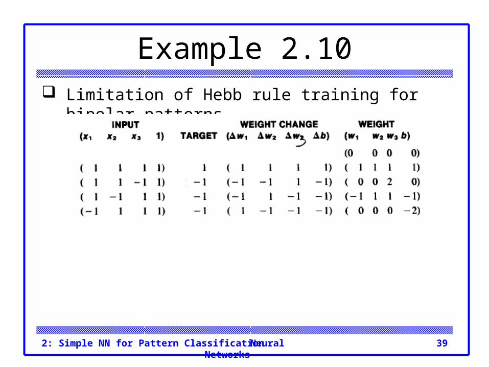
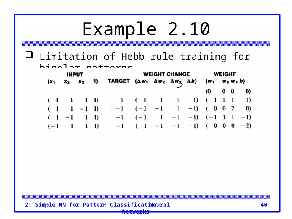
Example 2.10 Limitation of Hebb rule training for bipolar patterns.
Neural Networks2: Simple NN for Pattern Classification 40
Example 2.10 Limitation of Hebb rule training for bipolar patterns.
Neural Networks2: Simple NN for Pattern Classification 41
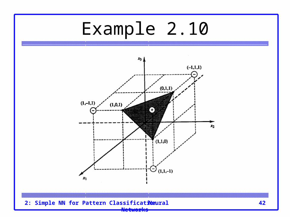
Example 2.10 Again, it is clear that the weights do not give the
correct output for the first input pattern. Figure 2.13 shows that the input points are linearly
separable; one possible plane, XI + x2 + x3 + (-2) = 0, to perform the separation is shown.
This plane corresponds to a weight vector of (1 1 1) and a bias of -2.
Neural Networks2: Simple NN for Pattern Classification 42
Example 2.10
Neural Networks2: Simple NN for Pattern Classification 43
PERCEPTRON The perceptron learning rule is a more powerful
learning rule than the Hebb rule. Under suitable assumptions, its iterative learning
procedure can be proved to converge to the correct weights, i.e., the weights that allow the net to produce the correct output value for each of the training input patterns.
Neural Networks2: Simple NN for Pattern Classification 44
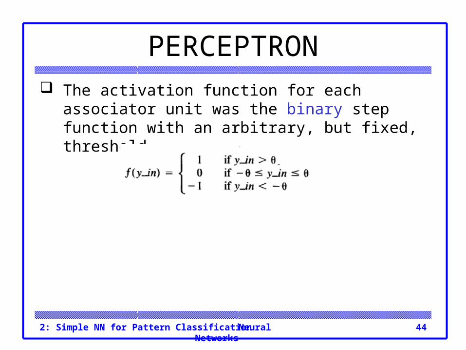
PERCEPTRON The activation function for each associator unit was
the binary step function with an arbitrary, but fixed, threshold.
Neural Networks2: Simple NN for Pattern Classification 45
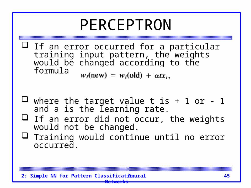
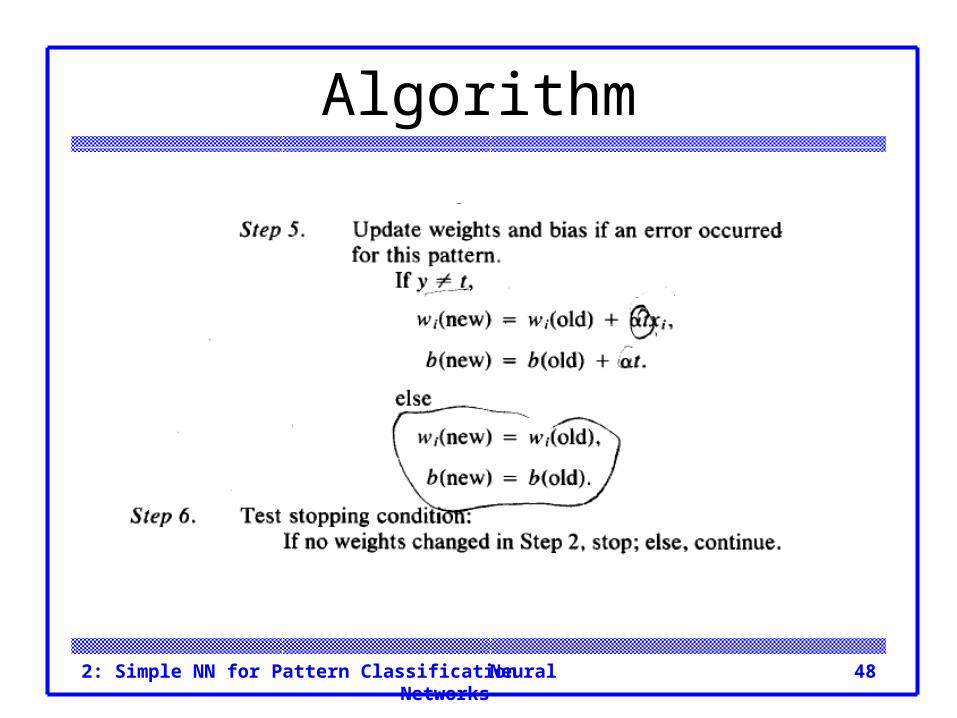
PERCEPTRON If an error occurred for a particular training input
pattern, the weights would be changed according to the formula
where the target value t is + 1 or - 1 and a is the learning rate.
If an error did not occur, the weights would not be changed.
Training would continue until no error occurred.
Neural Networks2: Simple NN for Pattern Classification 46
Architecture
Neural Networks2: Simple NN for Pattern Classification 47
Algorithm
Neural Networks2: Simple NN for Pattern Classification 48
Algorithm

Neural Networks2: Simple NN for Pattern Classification 49
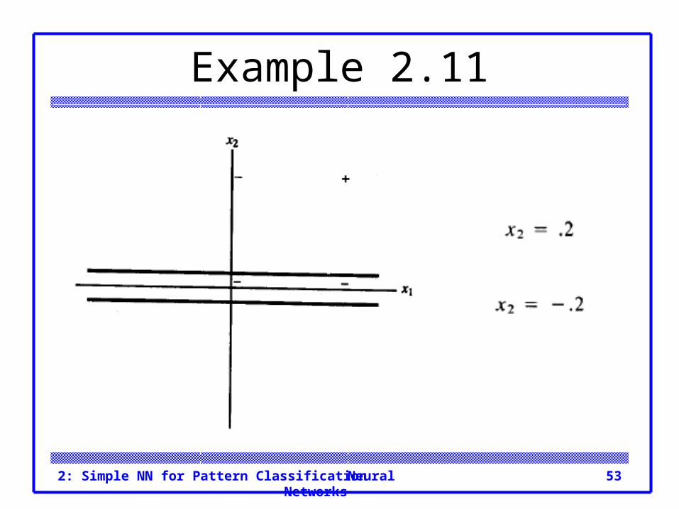
Algorithm Two separating lines:
Neural Networks2: Simple NN for Pattern Classification 50
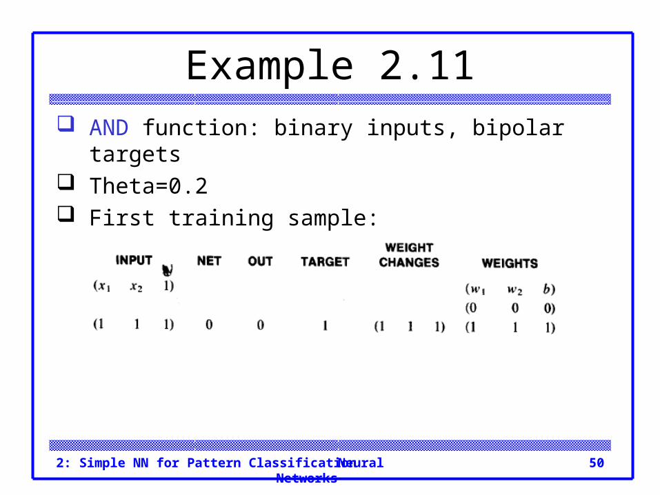
Example 2.11 AND function: binary inputs, bipolar targets Theta=0.2 First training sample:

Neural Networks2: Simple NN for Pattern Classification 51
Example 2.11
Neural Networks2: Simple NN for Pattern Classification 52
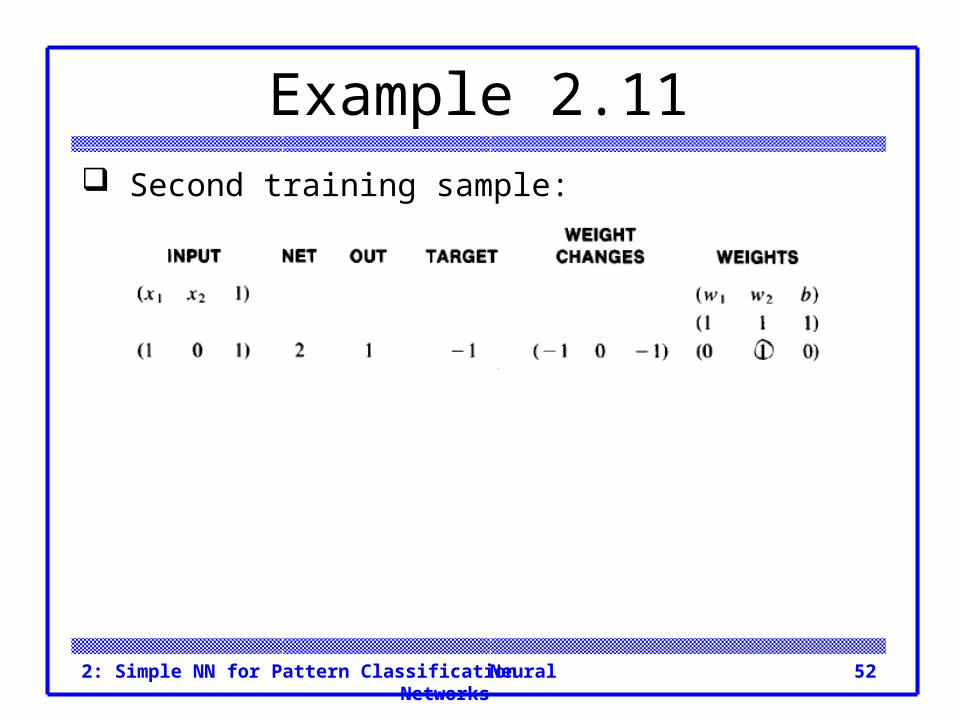
Example 2.11 Second training sample:
Neural Networks2: Simple NN for Pattern Classification 53
Example 2.11
Neural Networks2: Simple NN for Pattern Classification 54
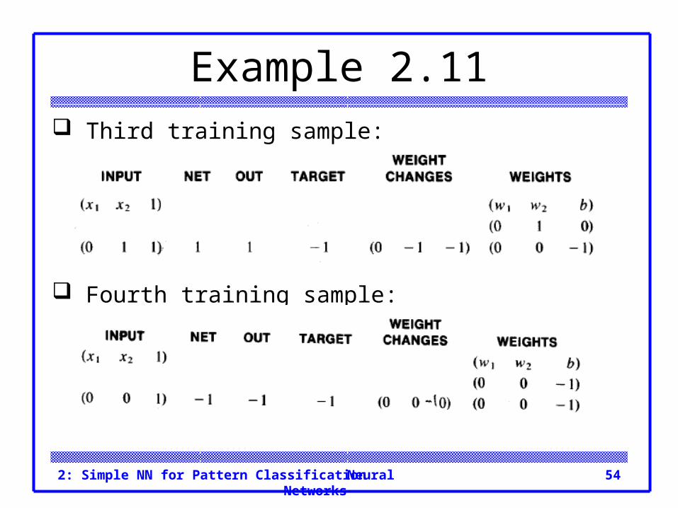
Example 2.11 Third training sample:
Fourth training sample:
Neural Networks2: Simple NN for Pattern Classification 55
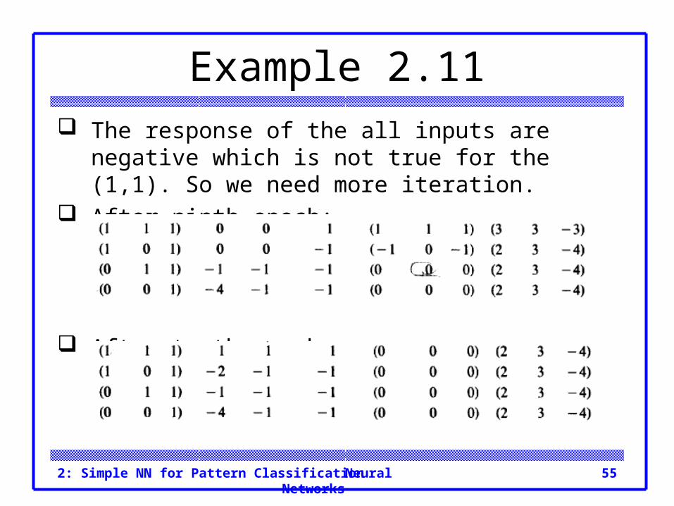
Example 2.11 The response of the all inputs are negative which is
not true for the (1,1). So we need more iteration. After ninth epoch:
After tenth epoch:
Neural Networks2: Simple NN for Pattern Classification 56
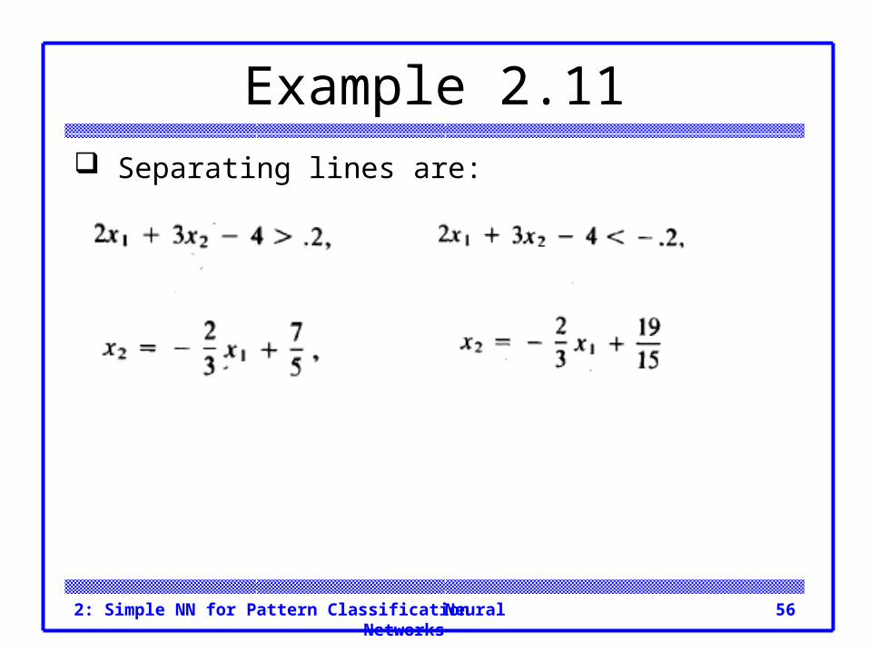
Example 2.11 Separating lines are:
Neural Networks2: Simple NN for Pattern Classification 57
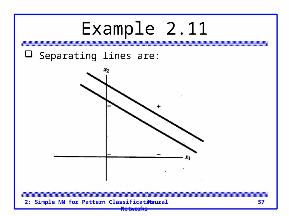
Example 2.11 Separating lines are:
Neural Networks2: Simple NN for Pattern Classification 58
Example 2.12 A Perceptron for the AND function: bipolar inputs
and targets. The training process Alpha=1 and threshold and
initial weights = 0.
Neural Networks2: Simple NN for Pattern Classification 59
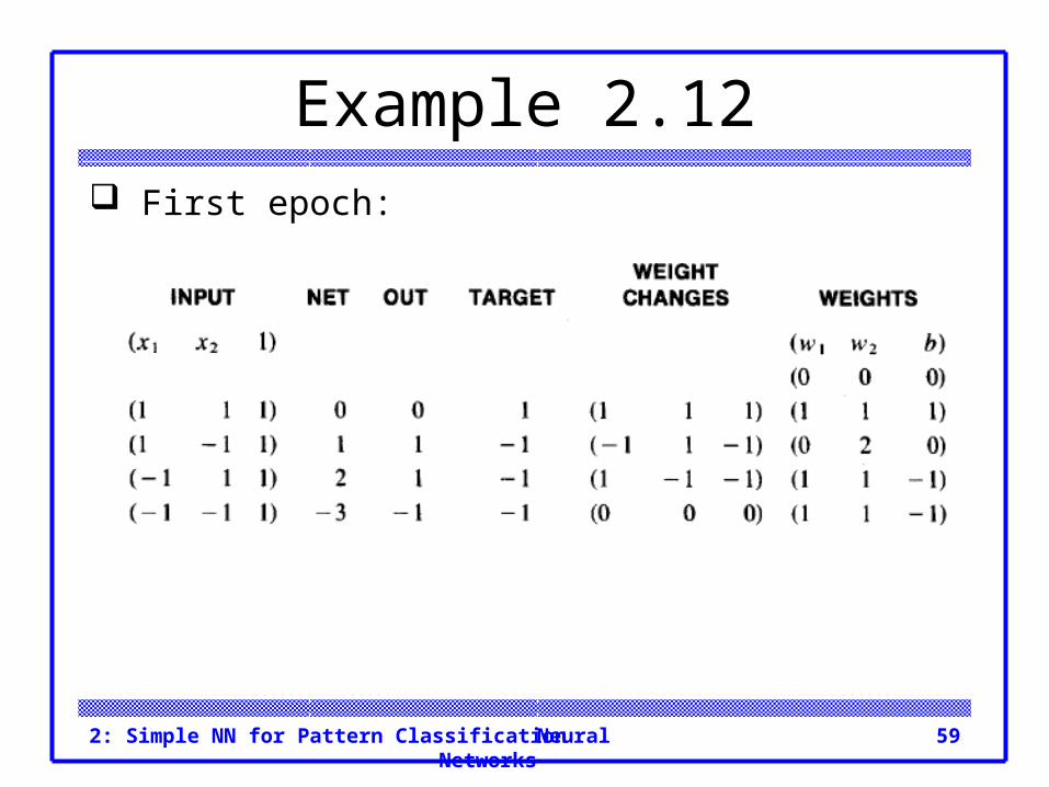
Example 2.12 First epoch:

Neural Networks2: Simple NN for Pattern Classification 60
Example 2.12 Second epoch:
the system was fully trained after the first epoch. Bipolar representation reduces number of epochs.
Neural Networks2: Simple NN for Pattern Classification 61
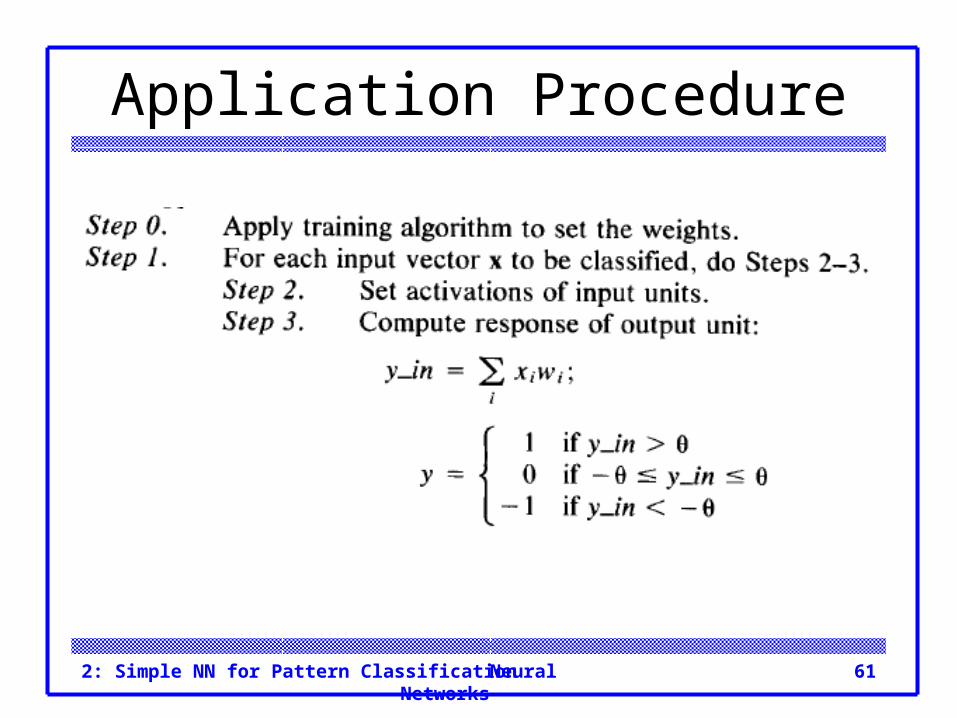
Application Procedure
Neural Networks2: Simple NN for Pattern Classification 62
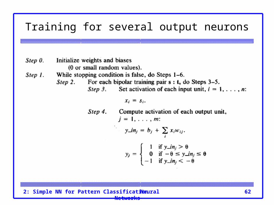
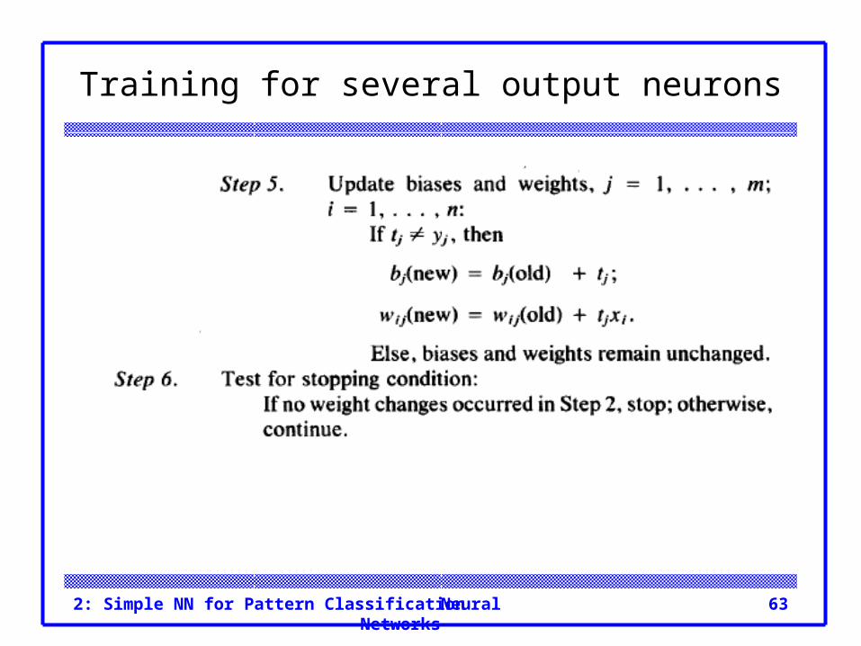
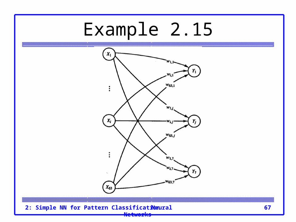
Training for several output neurons
Neural Networks2: Simple NN for Pattern Classification 63
Training for several output neurons
Neural Networks2: Simple NN for Pattern Classification 64
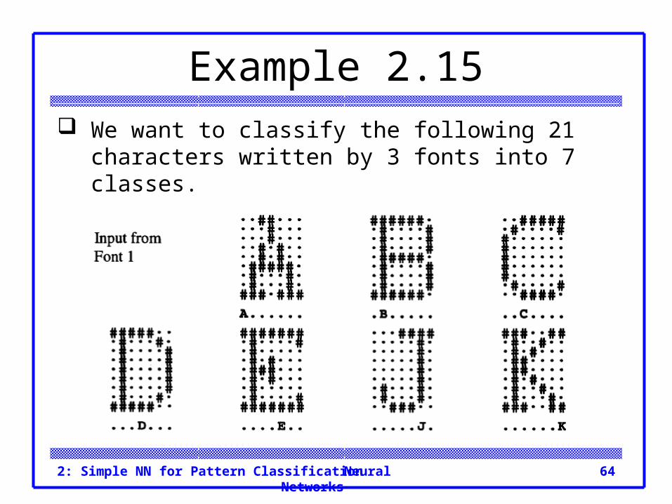
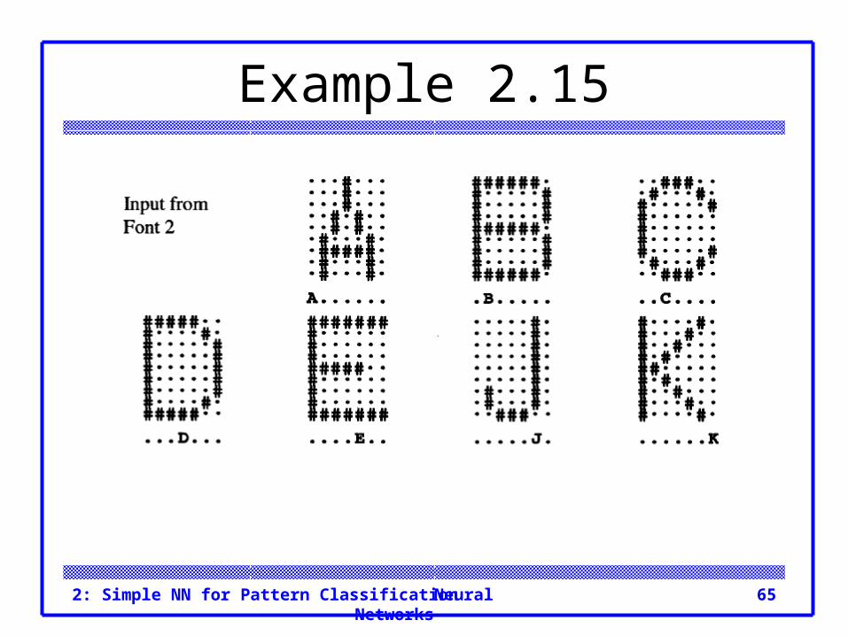
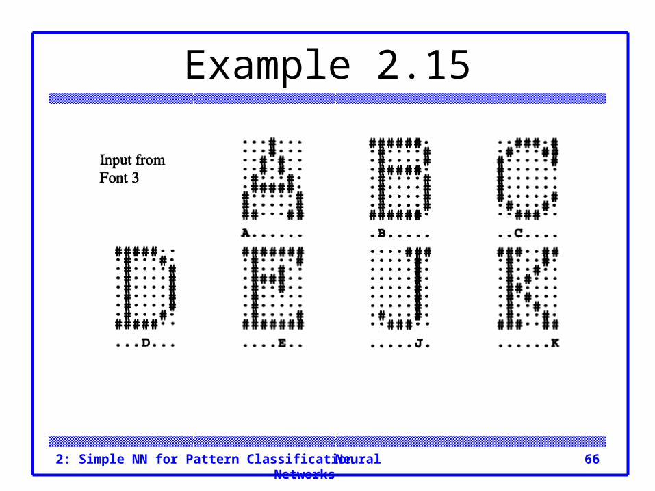
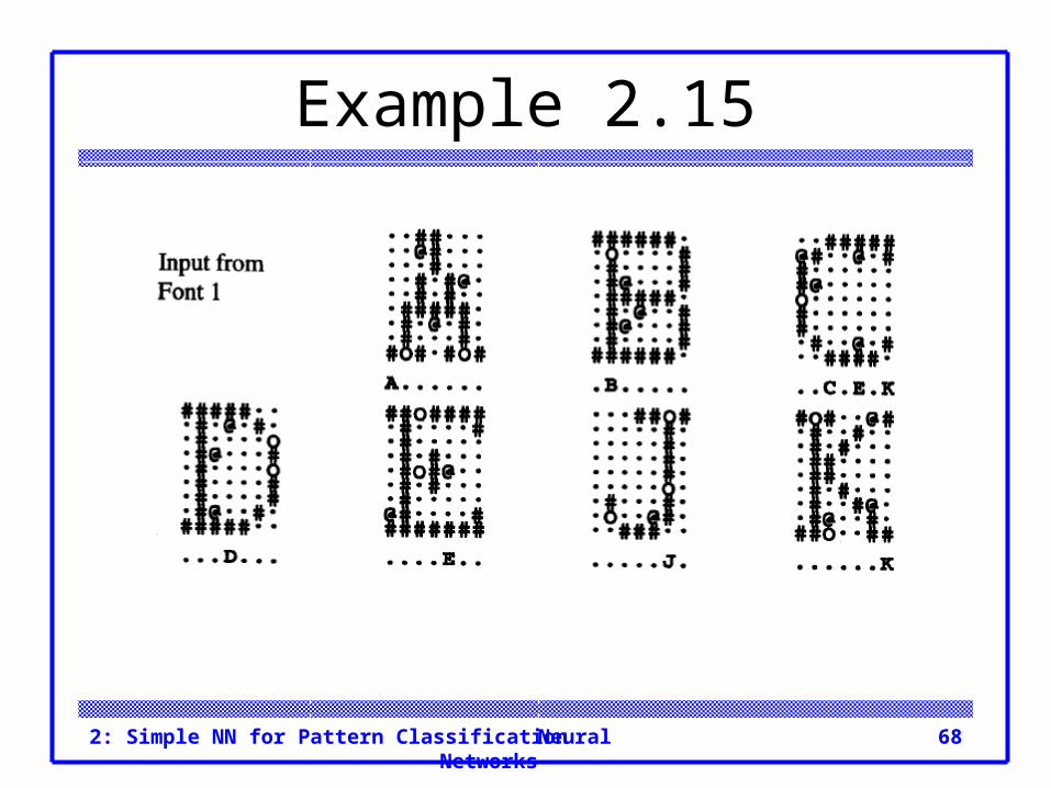
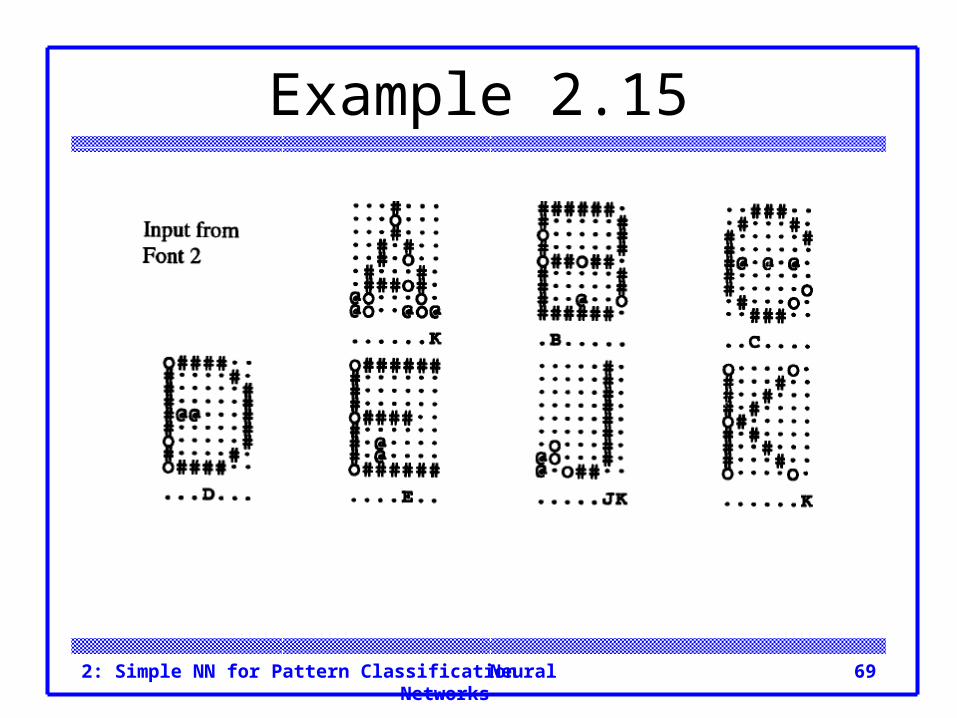
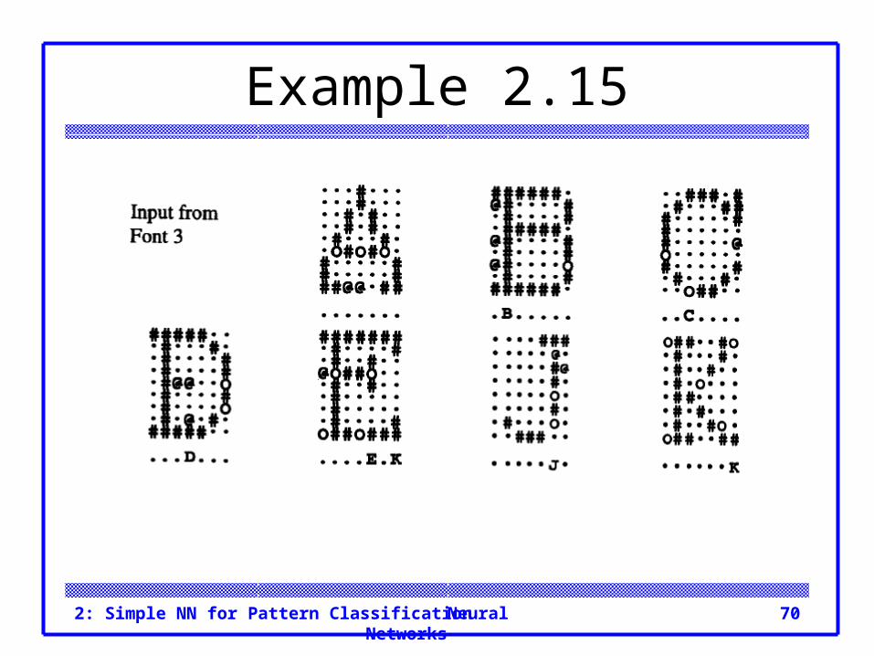
Example 2.15 We want to classify the following 21 characters
written by 3 fonts into 7 classes.
Neural Networks2: Simple NN for Pattern Classification 65
Example 2.15
Neural Networks2: Simple NN for Pattern Classification 66
Example 2.15
Neural Networks2: Simple NN for Pattern Classification 67
Example 2.15
Neural Networks2: Simple NN for Pattern Classification 68
Example 2.15
Neural Networks2: Simple NN for Pattern Classification 69
Example 2.15
Neural Networks2: Simple NN for Pattern Classification 70
Example 2.15
Neural Networks2: Simple NN for Pattern Classification 71
Adaline The ADALINE = ADAptive Linear Neuron. an ADALINE can be trained using the delta rule, also
known as the least mean squares (LMS) or Widrow-Hoff rule.
During training, the activation of the unit is its net input, i.e., the activation function is the identity function.
The learning rule minimizes the mean squared error between the activation and the target value.
Neural Networks2: Simple NN for Pattern Classification 72
Architecture
Neural Networks2: Simple NN for Pattern Classification 73
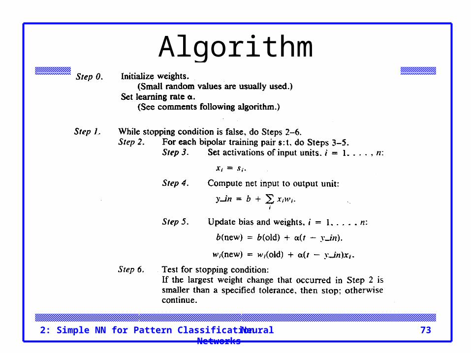
Algorithm
Neural Networks2: Simple NN for Pattern Classification 74
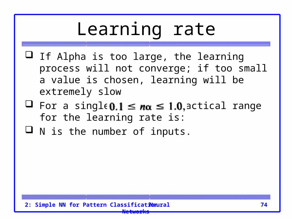
Learning rate If Alpha is too large, the learning process will not
converge; if too small a value is chosen, learning will be extremely slow
For a single neuron, a practical range for the learning rate is:
N is the number of inputs.
Neural Networks2: Simple NN for Pattern Classification 75
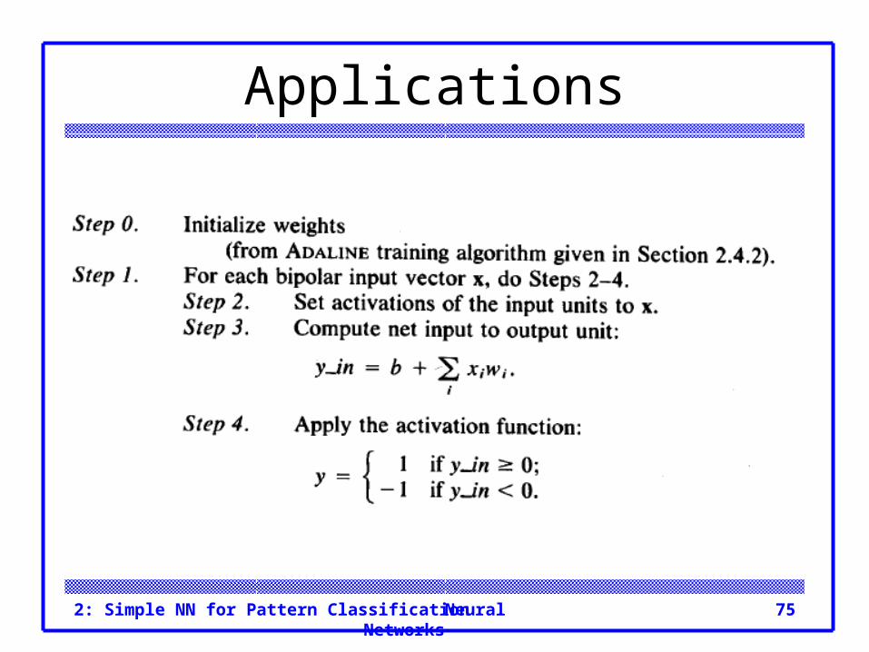
Applications
Neural Networks2: Simple NN for Pattern Classification 76
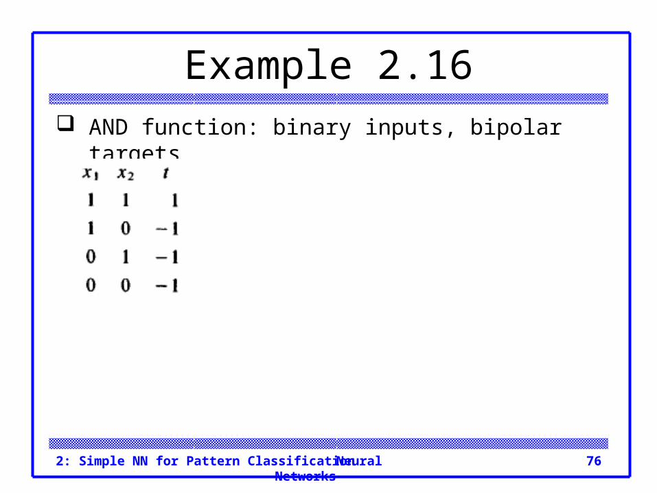
Example 2.16 AND function: binary inputs, bipolar targets
Neural Networks2: Simple NN for Pattern Classification 77
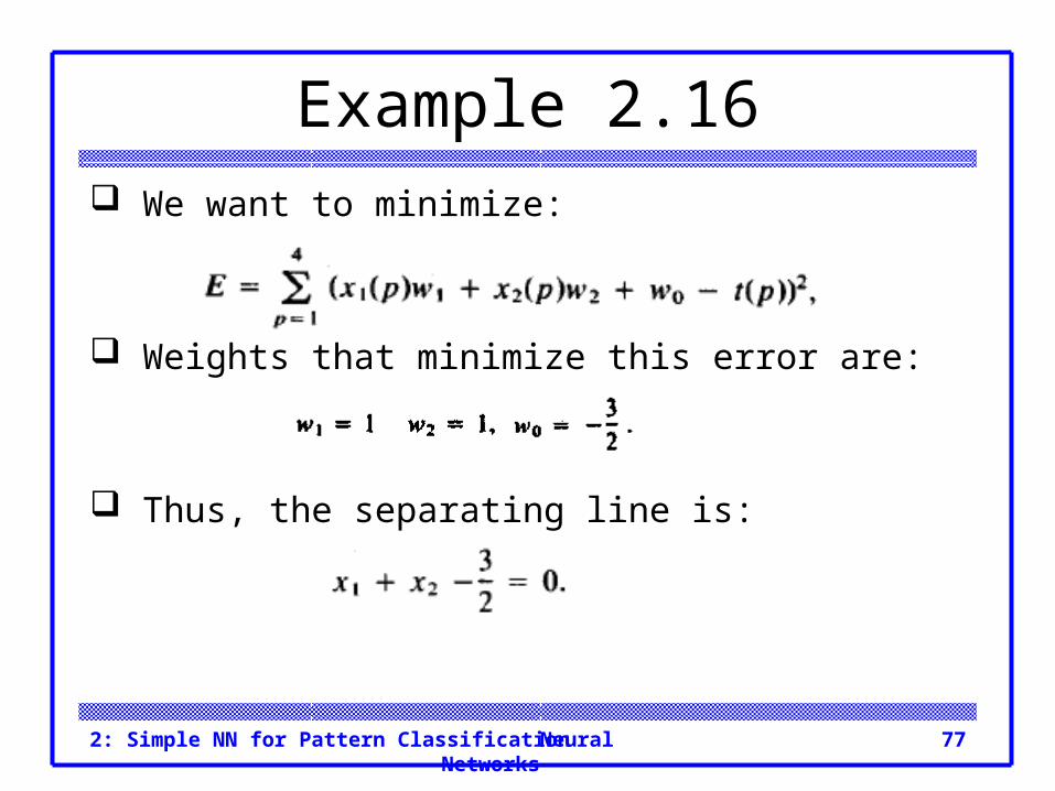
Example 2.16 We want to minimize:
Weights that minimize this error are:
Thus, the separating line is:
Neural Networks2: Simple NN for Pattern Classification 78
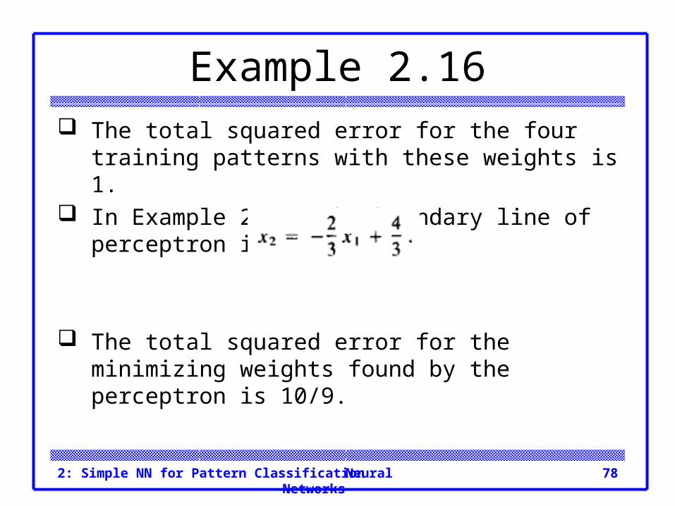
Example 2.16 The total squared error for the four training patterns
with these weights is 1. In Example 2.11, the boundary line of perceptron is:
The total squared error for the minimizing weights found by the perceptron is 10/9.
Neural Networks2: Simple NN for Pattern Classification 79
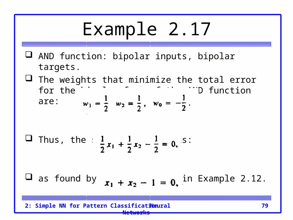
Example 2.17 AND function: bipolar inputs, bipolar targets. The weights that minimize the total error for the
bipolar form of the AND function are:
Thus, the separating line is:
as found by the perceptron in Example 2.12.
Neural Networks2: Simple NN for Pattern Classification 80
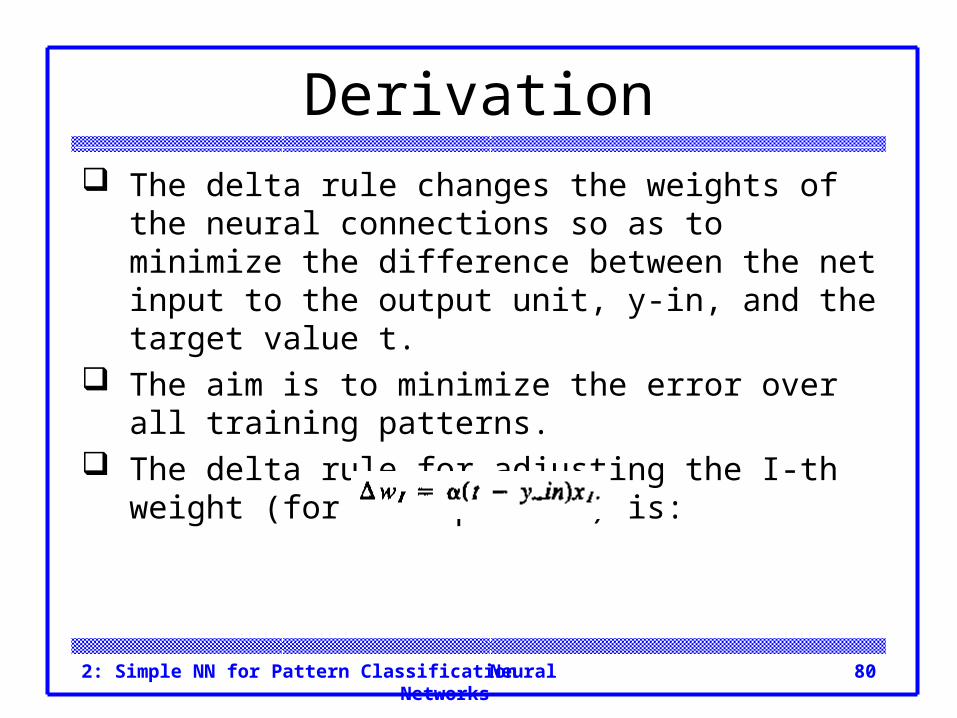
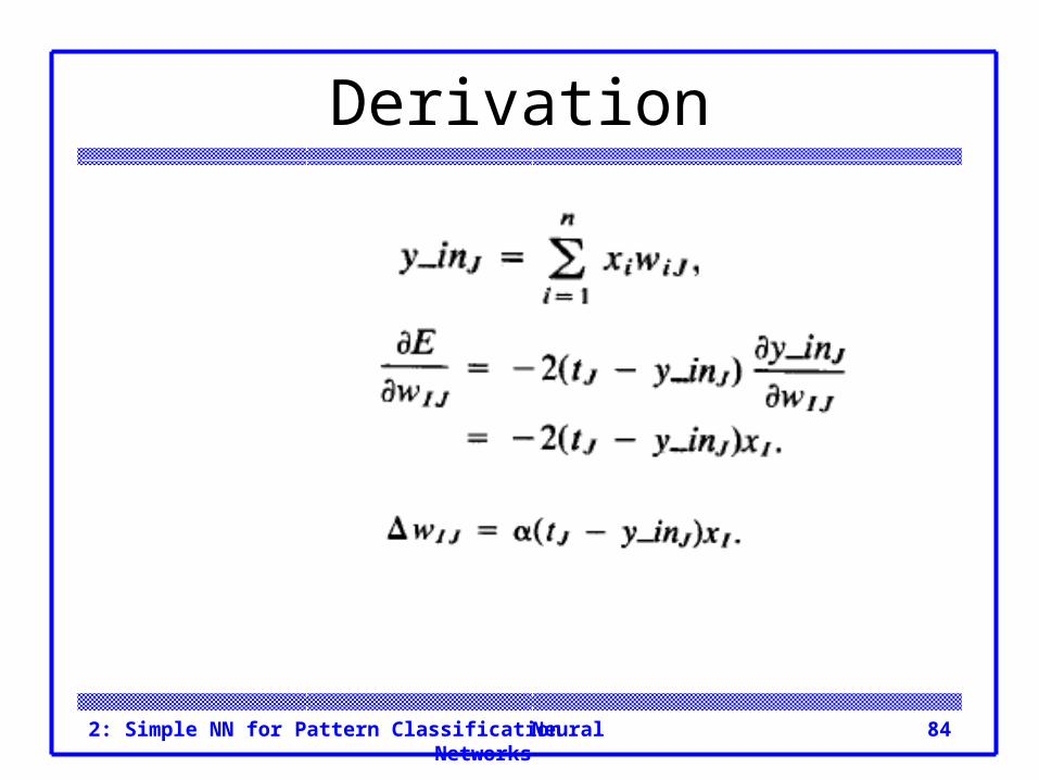
Derivation The delta rule changes the weights of the neural
connections so as to minimize the difference between the net input to the output unit, y-in, and the target value t.
The aim is to minimize the error over all training patterns.
The delta rule for adjusting the I-th weight (for each pattern) is:
Neural Networks2: Simple NN for Pattern Classification 81
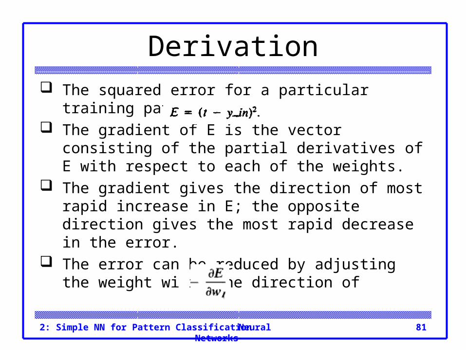
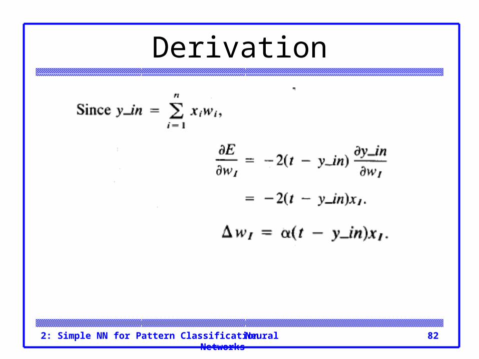
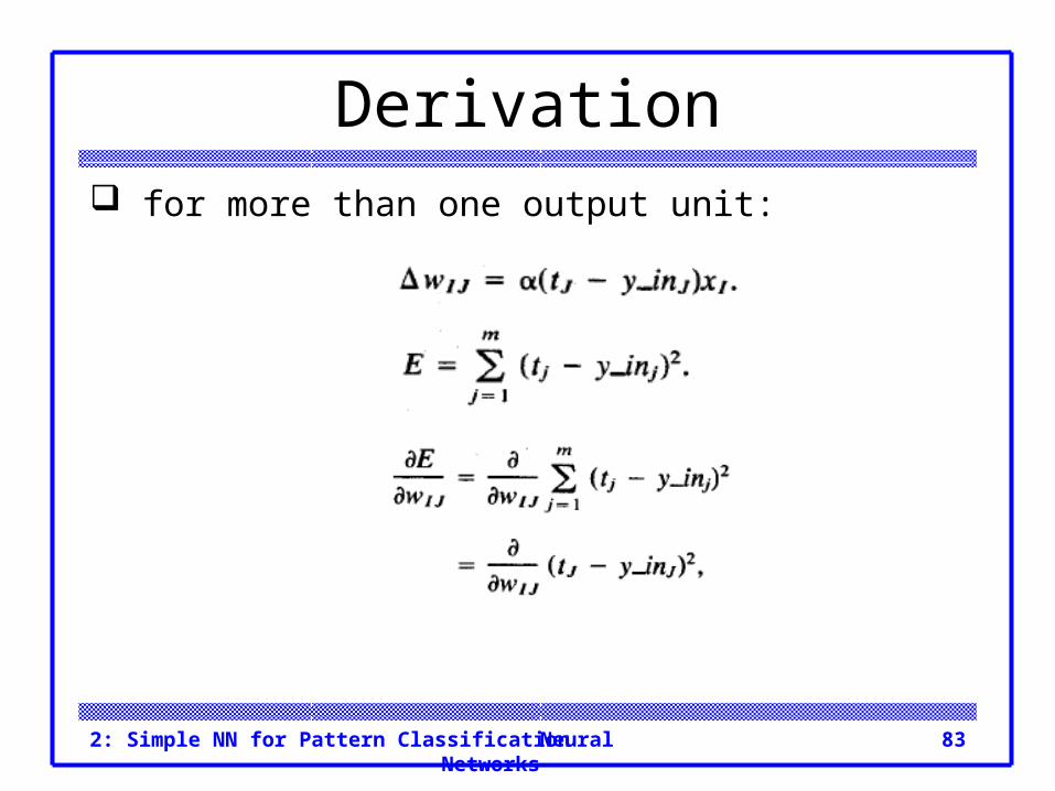
Derivation The squared error for a particular training pattern is:
The gradient of E is the vector consisting of the partial derivatives of E with respect to each of the weights.
The gradient gives the direction of most rapid increase in E; the opposite direction gives the most rapid decrease in the error.
The error can be reduced by adjusting the weight wi in the direction of
Neural Networks2: Simple NN for Pattern Classification 82
Derivation
Neural Networks2: Simple NN for Pattern Classification 83
Derivation for more than one output unit:
Neural Networks2: Simple NN for Pattern Classification 84
Derivation

Neural Networks2: Simple NN for Pattern Classification 85
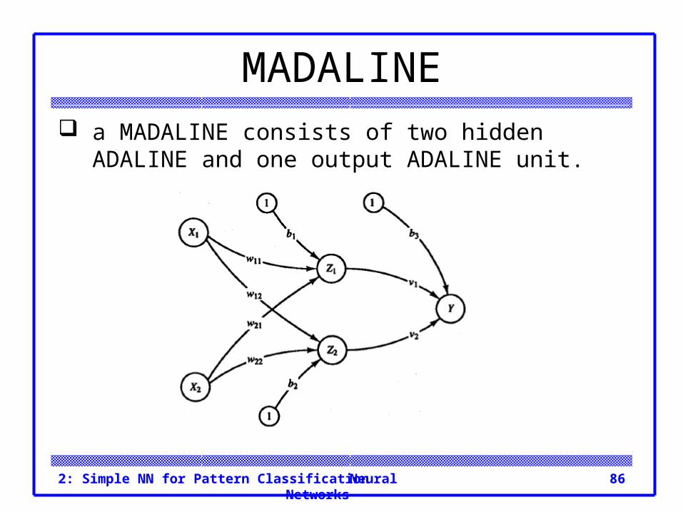
MADALINE a MADALINE consists of Many ADAptive Linear
Neurons arranged in a multilayer net.
Neural Networks2: Simple NN for Pattern Classification 86
MADALINE a MADALINE consists of two hidden ADALINE and
one output ADALINE unit.
Neural Networks2: Simple NN for Pattern Classification 87
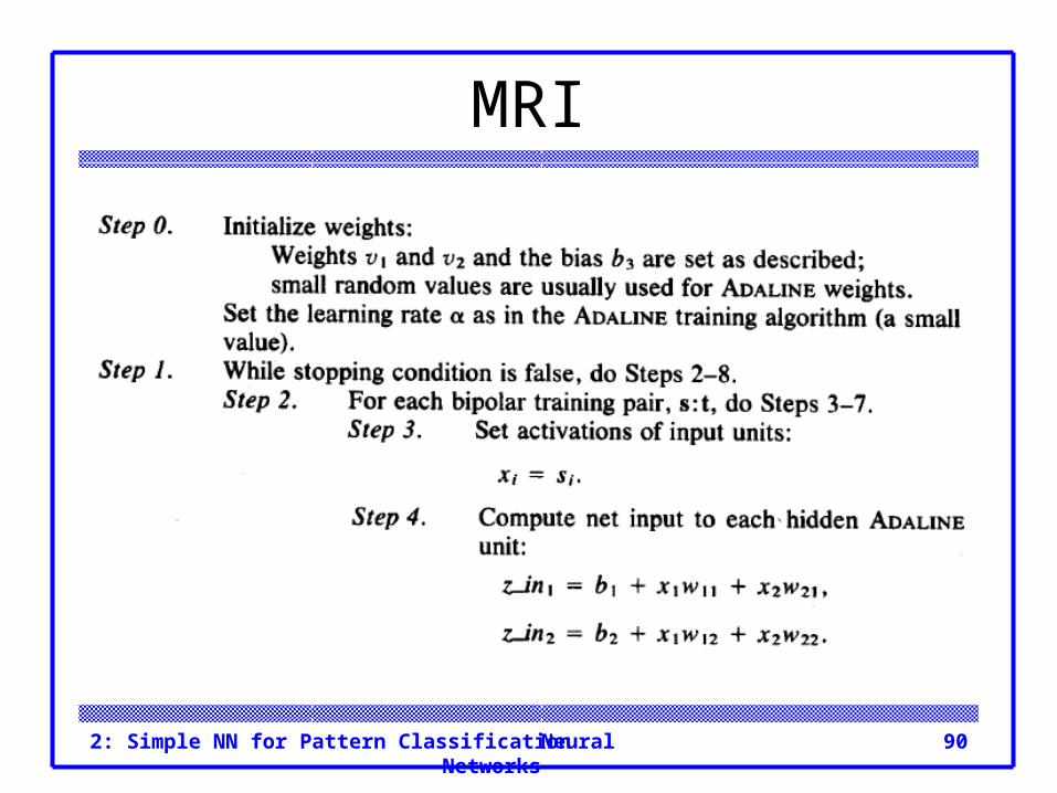
Algorithm In the MRI algorithm (the original form of MADALINE
training), only the weights for the hidden ADALINES are adjusted; the weights for the output unit are fixed.
The MRII algorithm provides a method for adjusting all weights in the net.
Neural Networks2: Simple NN for Pattern Classification 88
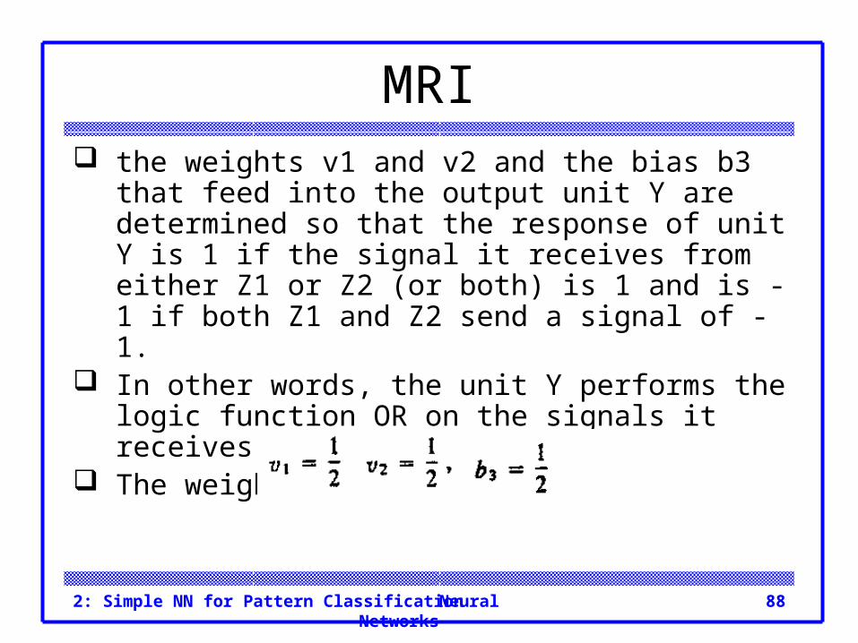
MRI the weights v1 and v2 and the bias b3 that feed into
the output unit Y are determined so that the response of unit Y is 1 if the signal it receives from either Z1 or Z2 (or both) is 1 and is - 1 if both Z1 and Z2 send a signal of - 1.
In other words, the unit Y performs the logic function OR on the signals it receives from Z1 and Z2.
The weights into Y are:

Neural Networks2: Simple NN for Pattern Classification 89
MRI The weights on the first hidden ADALINE (
) and the weights on the second hidden ADALINE ( ) are adjusted according to the algorithm.
The activation function for units ZI, Z2, and Y is:
Neural Networks2: Simple NN for Pattern Classification 90
MRI
Neural Networks2: Simple NN for Pattern Classification 91
MRI
Neural Networks2: Simple NN for Pattern Classification 92
MRI
Neural Networks2: Simple NN for Pattern Classification 93
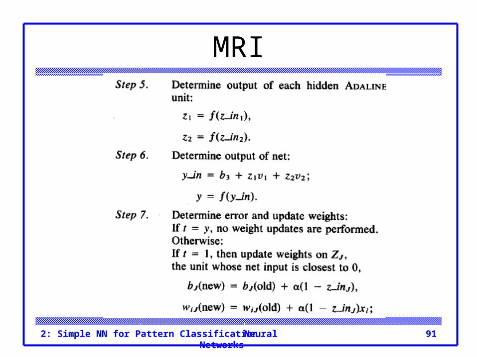
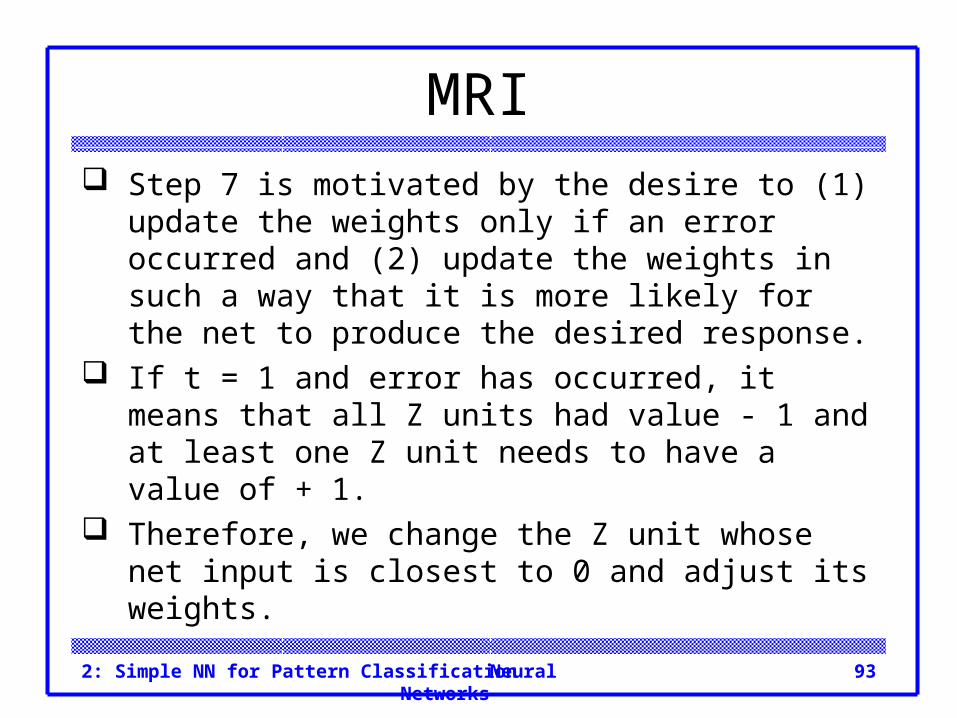
MRI Step 7 is motivated by the desire to (1) update the
weights only if an error occurred and (2) update the weights in such a way that it is more likely for the net to produce the desired response.
If t = 1 and error has occurred, it means that all Z units had value - 1 and at least one Z unit needs to have a value of + 1.
Therefore, we change the Z unit whose net input is closest to 0 and adjust its weights.
Neural Networks2: Simple NN for Pattern Classification 94
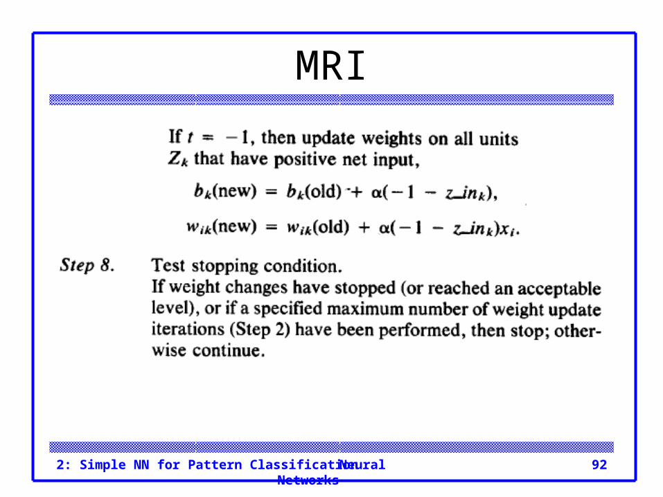
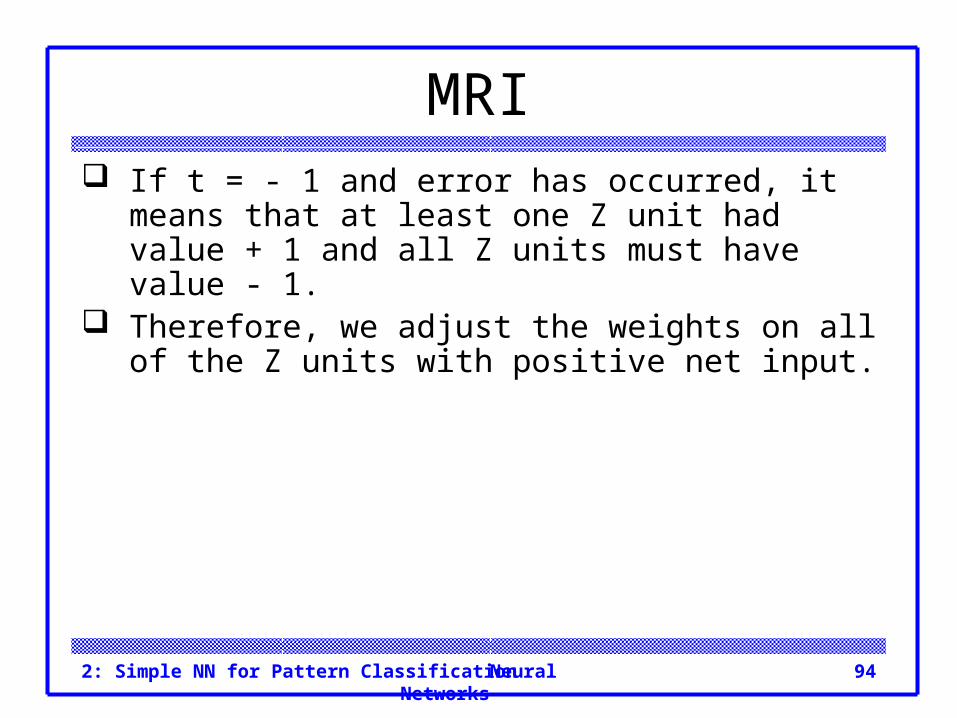
MRI If t = - 1 and error has occurred, it means that at
least one Z unit had value + 1 and all Z units must have value - 1.
Therefore, we adjust the weights on all of the Z units with positive net input.
Neural Networks2: Simple NN for Pattern Classification 95
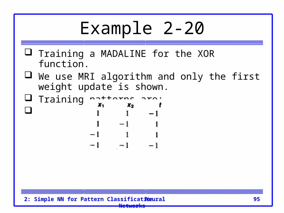
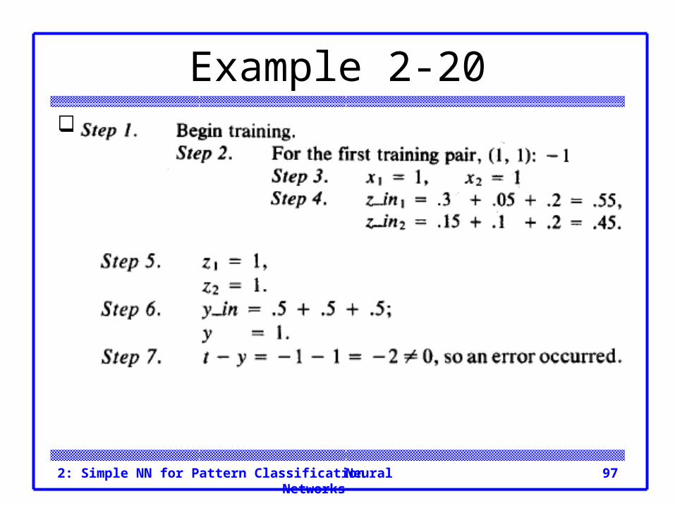
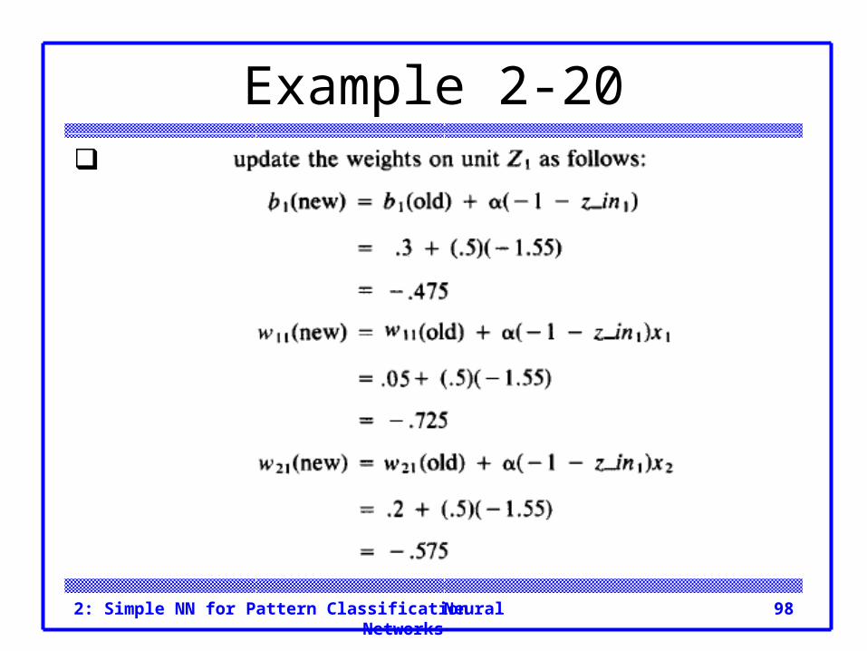
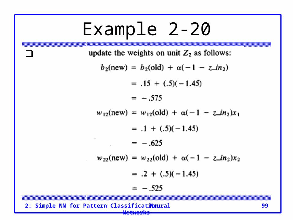
Example 2-20 Training a MADALINE for the XOR function. We use MRI algorithm and only the first weight
update is shown. Training patterns are:
Neural Networks2: Simple NN for Pattern Classification 96
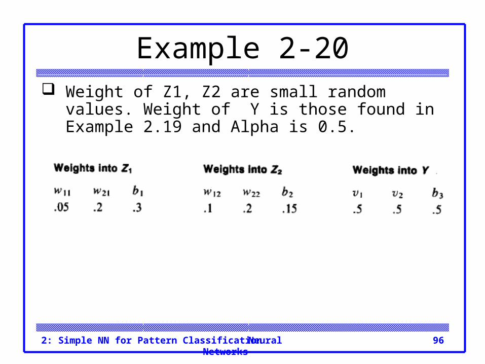
Example 2-20 Weight of Z1, Z2 are small random values. Weight of
Y is those found in Example 2.19 and Alpha is 0.5.
Neural Networks2: Simple NN for Pattern Classification 97
Example 2-20
Neural Networks2: Simple NN for Pattern Classification 98
Example 2-20
Neural Networks2: Simple NN for Pattern Classification 99
Example 2-20
Neural Networks2: Simple NN for Pattern Classification 100
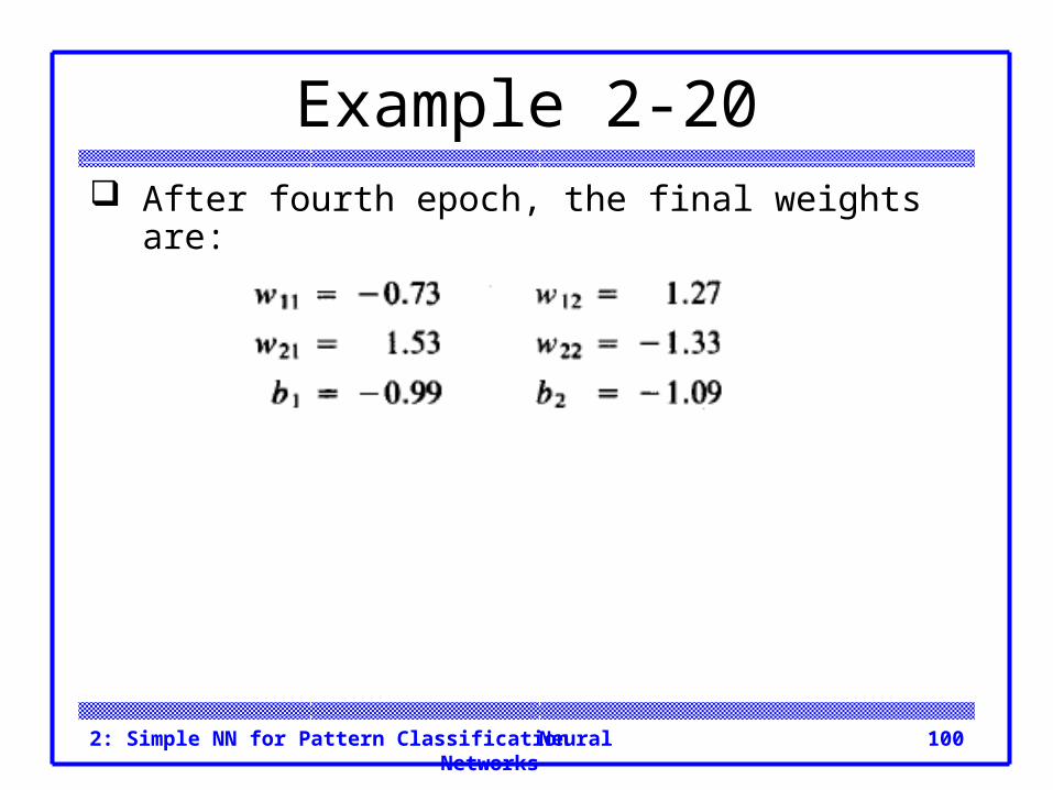
Example 2-20 After fourth epoch, the final weights are:
Neural Networks2: Simple NN for Pattern Classification 101
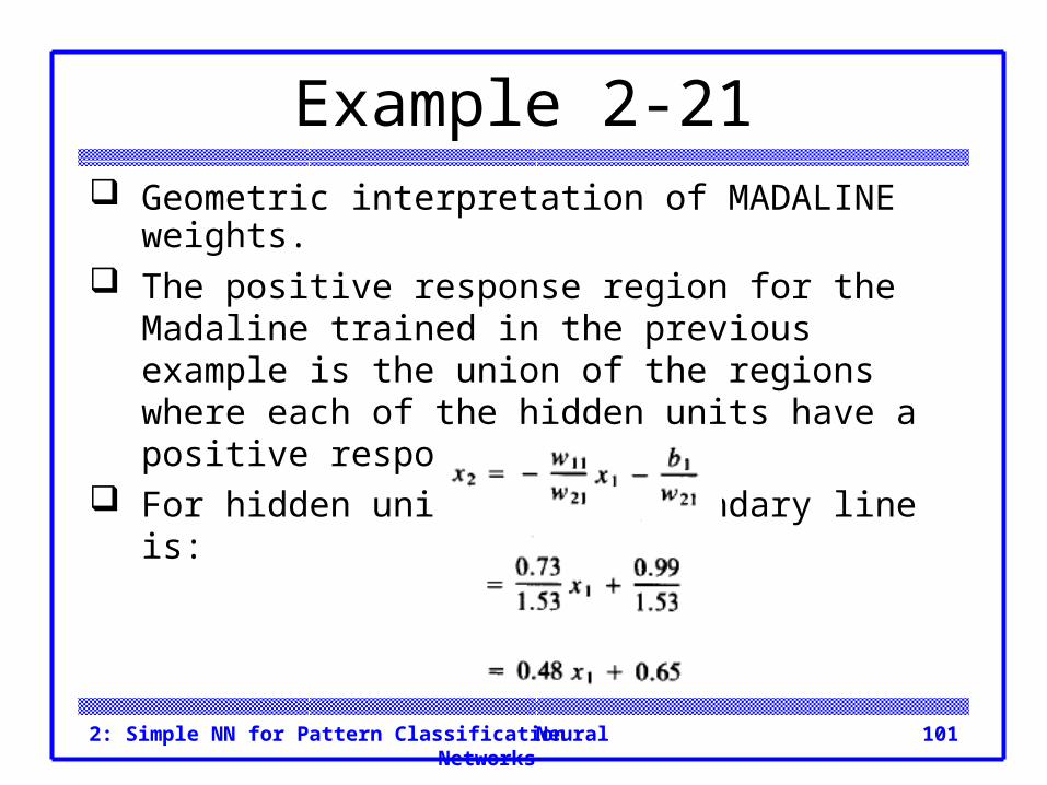
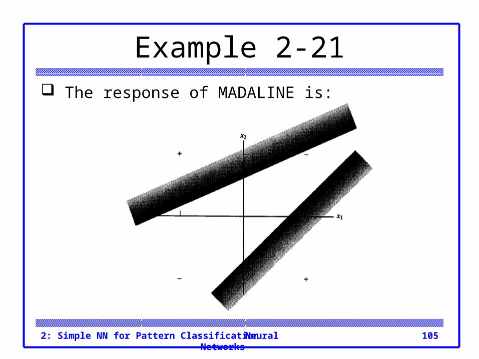
Example 2-21 Geometric interpretation of MADALINE weights. The positive response region for the Madaline
trained in the previous example is the union of the regions where each of the hidden units have a positive response.
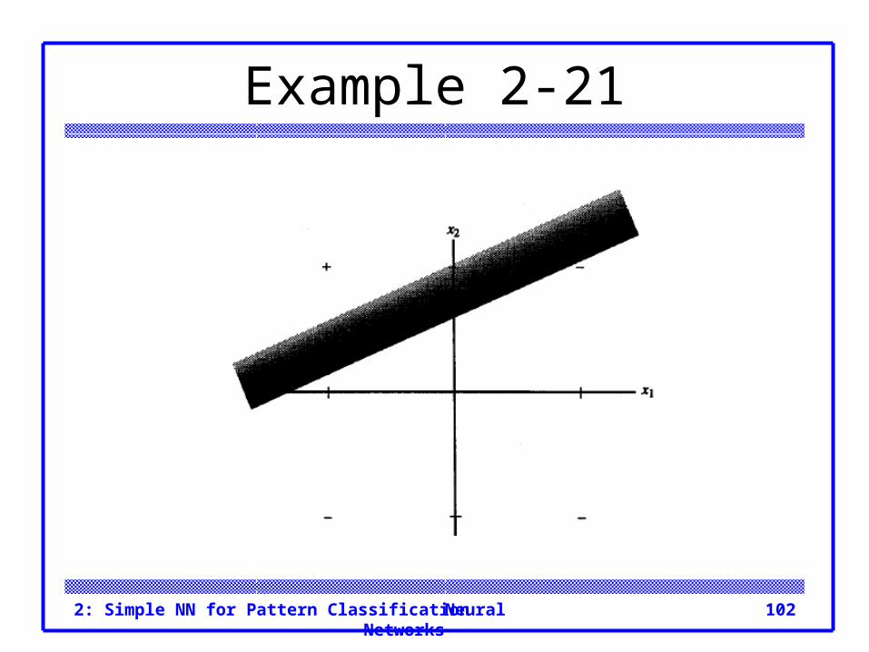
For hidden unit Z1, the boundary line is:
Neural Networks2: Simple NN for Pattern Classification 102
Example 2-21
Neural Networks2: Simple NN for Pattern Classification 103
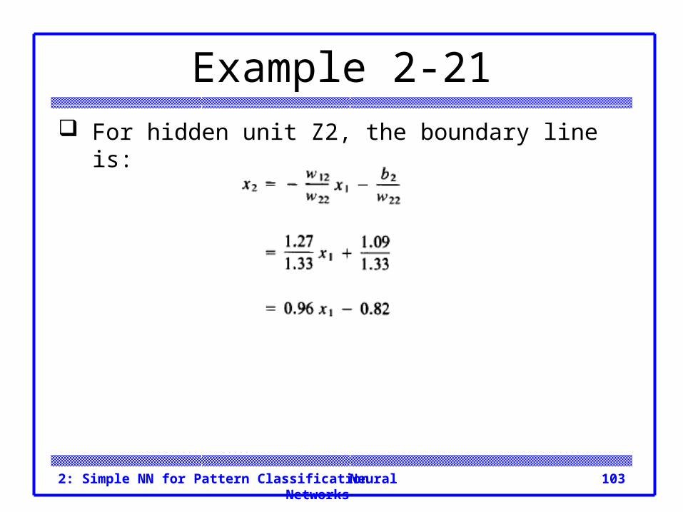
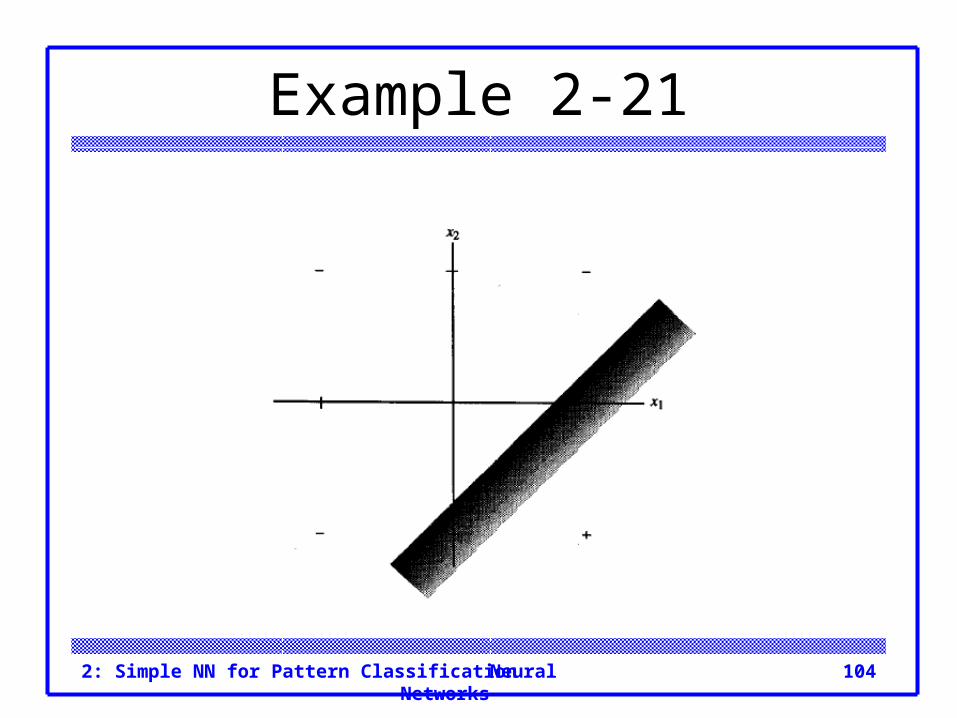
Example 2-21 For hidden unit Z2, the boundary line is:
Neural Networks2: Simple NN for Pattern Classification 104
Example 2-21
Neural Networks2: Simple NN for Pattern Classification 105
Example 2-21 The response of MADALINE is: