knowledge discovery in databases ii - uni-muenchen.de · 2015-10-21 · knowledge discovery in...
TRANSCRIPT
DATABASESYSTEMSGROUP
Knowledge Discovery in Databases IIWinter Term 2015/2016
Knowledge Discovery in Databases II: High-Dimensional Data
Ludwig-Maximilians-Universität MünchenInstitut für Informatik
Lehr- und Forschungseinheit für Datenbanksysteme
Lectures : Dr Eirini Ntoutsi, PD Dr Matthias SchubertTutorials: PD Dr Matthias Schubert
Script © 2015 Eirini Ntoutsi, Matthias Schubert, Arthur Zimek
http://www.dbs.ifi.lmu.de/cms/Knowledge_Discovery_in_Databases_II_(KDD_II)
Lecture 2: Volume: High-Dimensional Data: Feature Selection
1

DATABASESYSTEMSGROUP
Outline
1. Introduction and challenges of high dimensionality
2. Feature Selection
3. Feature Reduction and Metric Learning
4. Clustering in High-Dimensional Data
Knowledge Discovery in Databases II: High-Dimensional Data 2
DATABASESYSTEMSGROUP
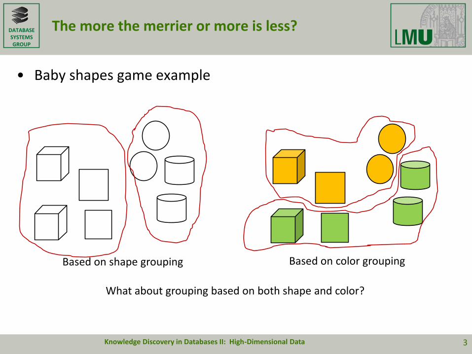
The more the merrier or more is less?
• Baby shapes game example
Knowledge Discovery in Databases II: High-Dimensional Data 3
Based on shape grouping Based on color grouping
What about grouping based on both shape and color?

DATABASESYSTEMSGROUP
Examples of High-Dimensional Data 1/2
• Image data
low-level image descriptors(color histograms, textures, shape information ...)
If each pixel a feature, a 64x64 image 4,096 features
Regional descriptors
Between 16 and 1,000 features
• Metabolome data
feature = concentration of one metabolite
The term metabolite usually restricted to small molecules, that are intermediates and products of metabolism.
The Human Metabolome Database contains 41,993 metabolite entries
Bavaria newborn screening (For each newborn in Bavaria, the blood concentrations of 43 metabolites are measured in the first 48 hours after birth)
between 50 and 2,000 features
... ...
Knowledge Discovery in Databases II: High-Dimensional Data 4
DATABASESYSTEMSGROUP
Examples of High-Dimensional Data 2/2
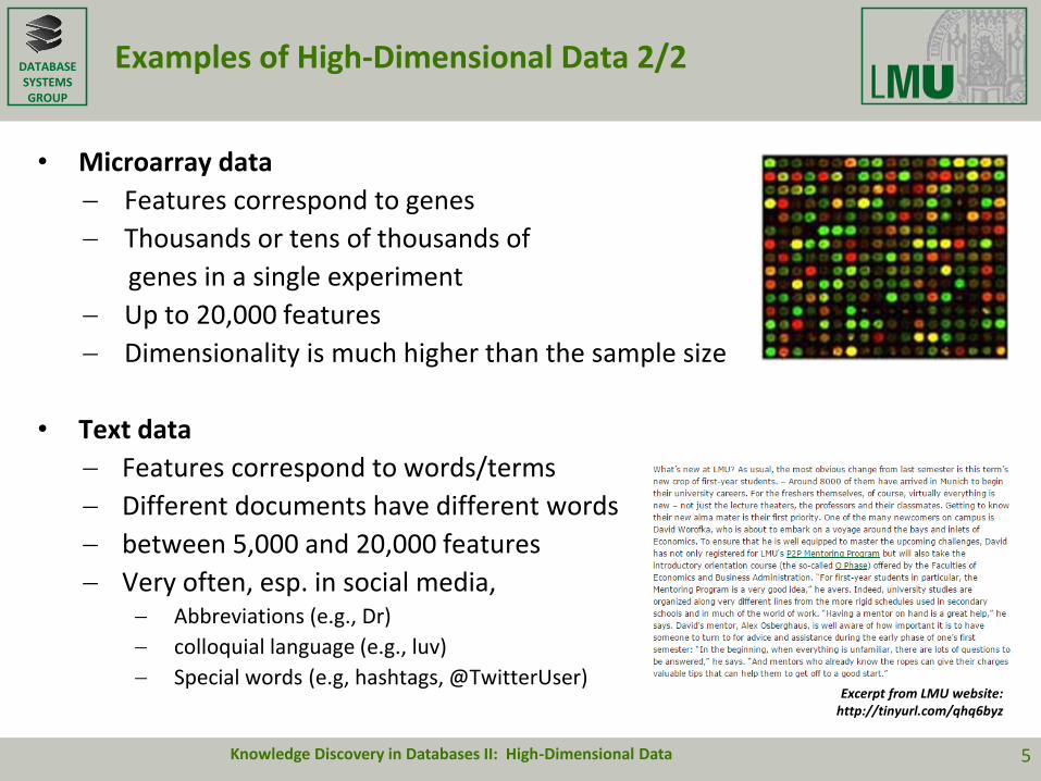
• Microarray data
Features correspond to genes
Thousands or tens of thousands of
genes in a single experiment
Up to 20,000 features
Dimensionality is much higher than the sample size
• Text data
Features correspond to words/terms
Different documents have different words
between 5,000 and 20,000 features
Very often, esp. in social media, Abbreviations (e.g., Dr)
colloquial language (e.g., luv)
Special words (e.g, hashtags, @TwitterUser)
Knowledge Discovery in Databases II: High-Dimensional Data 5
Excerpt from LMU website:http://tinyurl.com/qhq6byz

DATABASESYSTEMSGROUP
Challenges due to high dimensionality 1/5
• Curse of Dimensionality
– Distance to the nearest and the farthest neighbor converge
– The likelihood that a data object is located on the margin of the data space exponentially increases with the dimensionality
0 1
1
0 1 PFS = 11 = 1
Pcore = 0.81 = 0.8
Pmargin = 1 – 0.8 = 0.2
feature space (FS)
core
margin: 0.1
nearestNeighborDist
farthestNeighborDist 1
1D:
PFS = 12 = 1
Pcore = 0.82 = 0.64
Pmargin = 1 – 0.64 = 0.36
2D:
PFS = 13 = 1
Pcore = 0.83 = 0.512
Pmargin = 1 – 0.512 = 0.488
3D:
10D: PFS = 110 = 1
Pcore = 0.810 = 0.107
Pmargin = 1-0.107=0.893
Knowledge Discovery in Databases II: High-Dimensional Data 6

DATABASESYSTEMSGROUP
Challenges due to high dimensionality 2/5
• Pairwise distances example: sample of 105 instances drawn from a uniform [0, 1] distribution, normalized (1/ sqrt(d)).
Knowledge Discovery in Databases II: High-Dimensional Data 7
Source: Tutorial on Outlier Detection in High-Dimensional Data, Zimek et al, ICDM 2012
DATABASESYSTEMSGROUP
Challenges due to high dimensionality 3/5
Further explanation of the Curse of Dimensionality:
• Consider the feature space of d relevant features for a given application
=> truly similar objects display small distances in most features
• Now add d*x additional features being independent of the initial feature space
• With increasing x the distance in the independent subspace will dominate the distance in the complete feature space
How many relevant features must by similar to indicate object similarity?
How many relevant features must be dissimilar to indicate dissimilarity?
With increasing dimensionality the likelihood that two objects are similar in every respect gets smaller.
Knowledge Discovery in Databases II: High-Dimensional Data 8
DATABASESYSTEMSGROUP
Challenges due to high dimensionality 4/5
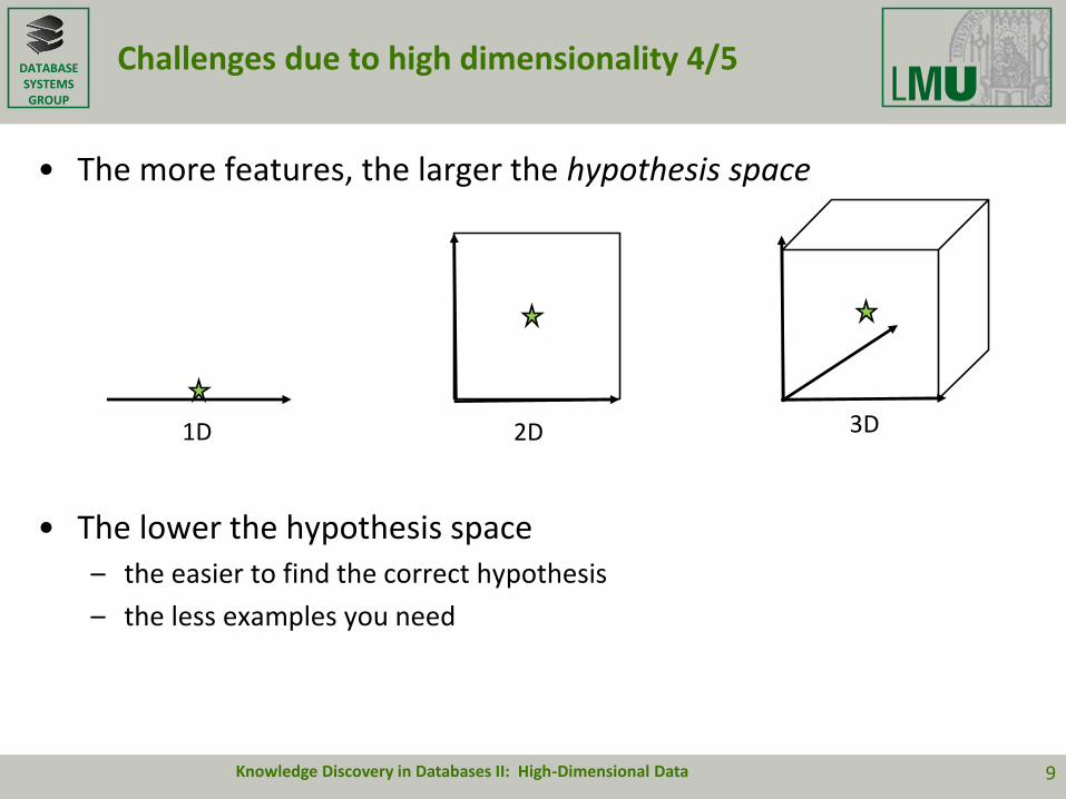
• The more features, the larger the hypothesis space
• The lower the hypothesis space – the easier to find the correct hypothesis
– the less examples you need
Knowledge Discovery in Databases II: High-Dimensional Data 9
1D 2D 3D
DATABASESYSTEMSGROUP
Challenges due to high dimensionality 5/5
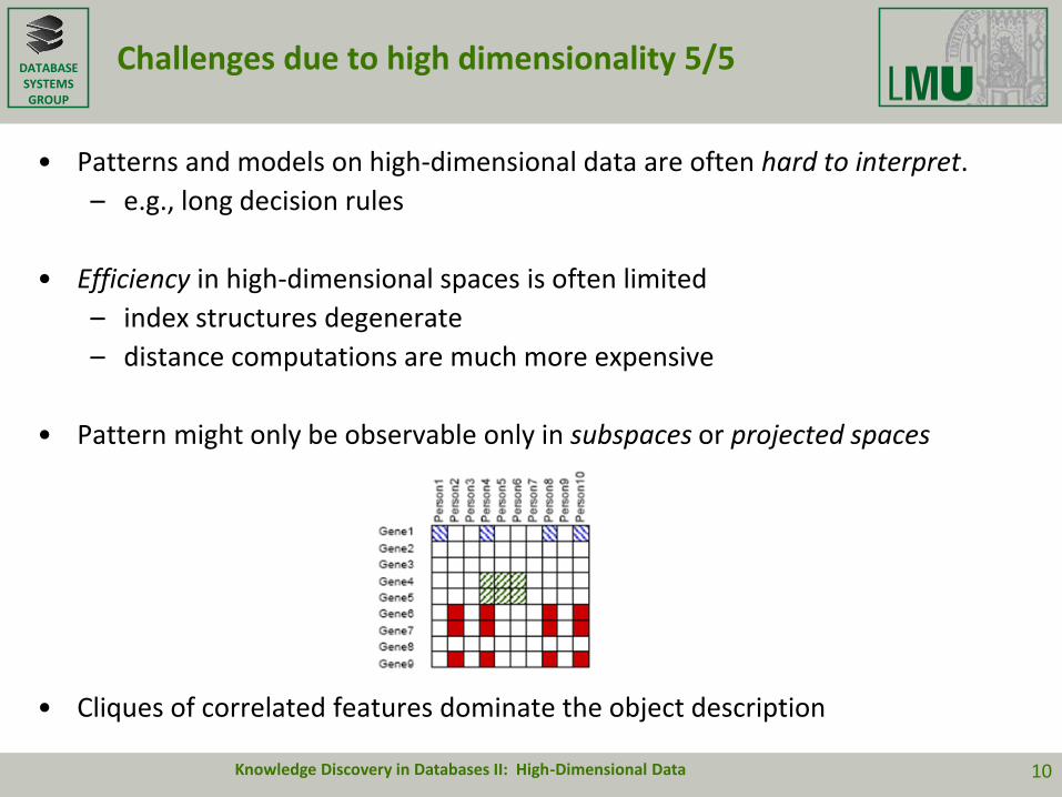
• Patterns and models on high-dimensional data are often hard to interpret.
– e.g., long decision rules
• Efficiency in high-dimensional spaces is often limited
– index structures degenerate
– distance computations are much more expensive
• Pattern might only be observable only in subspaces or projected spaces
• Cliques of correlated features dominate the object description
Knowledge Discovery in Databases II: High-Dimensional Data 10
DATABASESYSTEMSGROUP
Outline
1. Introduction and challenges of high dimensionality
2. Feature Selection
3. Feature Reduction and Metric Learning
4. Clustering in High-Dimensional Data
Knowledge Discovery in Databases II: High-Dimensional Data 11

DATABASESYSTEMSGROUP
Feature selection
• A task to remove irrelevant and/or redundant features
– Irrelevant features: not useful for a given task
• Relevant vs irrelevant
– Redundant features: a relevant feature may be redundant in the presence of another relevant feature with which it is strongly correlated.
• Deleting irrelevant and redundant features can improve the efficiency as well as the quality of the found methods and patterns.
• New feature space: Delete all useless features from the original feature space.
• Feature selection ≠ Dimensionality reduction
• Feature selection ≠ Feature extraction
Knowledge Discovery in Databases II: High-Dimensional Data 12

DATABASESYSTEMSGROUP
Irrelevant and redundant features (unsupervised learning case)
• Irrelevance • Redundancy
Knowledge Discovery in Databases II: High-Dimensional Data 13
Feature y is irrelevant, because if we omit x, we have only one cluster, which is uninteresting.
Features x and y are redundant, because x provides the same information as feature y with regard to discriminating the two clusters
Source: Feature Selection for Unsupervised Learning, Dy and Brodley, Journal of Machine Learning Research 5 (2004)

DATABASESYSTEMSGROUP
Irrelevant and redundant features (supervised learning case)
• Irrelevance
• Redundancy
Knowledge Discovery in Databases II: High-Dimensional Data 14
Feature y separates well the two classes.Feature x is irrelevant.Its addition “destroys” the class separation.
Features x and y are redundant.
Source: http://www.kdnuggets.com/2014/03/machine-learning-7-pictures.html
• Individually irrelevant, together relevant

DATABASESYSTEMSGROUP
Problem definition
• Input: Vector space F =d1×..× dn with dimensions D ={d1,,..,dn}.
• Output: a minimal subspace M over dimensions D` D which is optimal for a giving data mining task.
– Minimality increases the efficiency, reduces the effects of the curse of dimensionality and increases interpretability.
Challenges:
• Optimality depends on the given task
• There are 2d possible solution spaces (exponential search space)
• There is often no monotonicity in the quality of subspace
(Features might only be useful in combination with certain other features)
For many popular criteria, feature selection is an exponential problem
Most algorithms employ search heuristics
Knowledge Discovery in Databases II: High-Dimensional Data 15
DATABASESYSTEMSGROUP
2 main components
1. Feature subset generation– Single dimensions
– Combinations of dimensions (subpaces)
2. Feature subset evaluation– Importance scores like information gain, χ2
– Performance of a learning algorithm
Knowledge Discovery in Databases II: High-Dimensional Data 16

DATABASESYSTEMSGROUP
Feature selection methods 1/4
• Filter methods Explores the general characteristics of the data, independent of the learning
algorithm.
• Wrapper methods– The learning algorithm is used for the evaluation of the subspace
• Embedded methods– The feature selection is part of the learning algorithm
Knowledge Discovery in Databases II: High-Dimensional Data 17
DATABASESYSTEMSGROUP
Feature selection methods 2/4
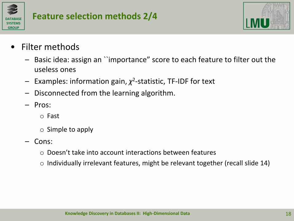
• Filter methods– Basic idea: assign an ``importance” score to each feature to filter out the
useless ones
– Examples: information gain, χ2-statistic, TF-IDF for text
– Disconnected from the learning algorithm.
– Pros:
o Fast
o Simple to apply
– Cons:
o Doesn’t take into account interactions between features
o Individually irrelevant features, might be relevant together (recall slide 14)
Knowledge Discovery in Databases II: High-Dimensional Data 18
DATABASESYSTEMSGROUP
Feature selection methods 3/4
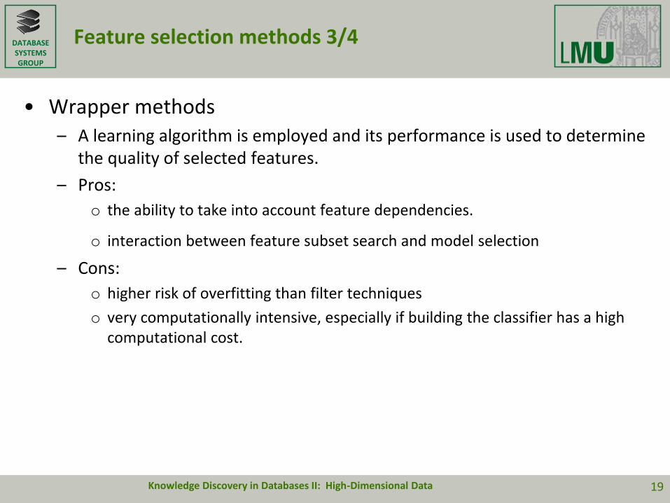
• Wrapper methods– A learning algorithm is employed and its performance is used to determine
the quality of selected features.
– Pros:
o the ability to take into account feature dependencies.
o interaction between feature subset search and model selection
– Cons:
o higher risk of overfitting than filter techniques
o very computationally intensive, especially if building the classifier has a high computational cost.
Knowledge Discovery in Databases II: High-Dimensional Data 19

DATABASESYSTEMSGROUP
Feature selection methods 4/4
• Embedded methods– Such methods integrate the feature selection in model building
– Example: decision tree induction algorithm: at each decision node, a feature has to be selected.
– Pros:
o less computationally intensive than wrapper methods.
– Cons:
o specific to a learning method
Knowledge Discovery in Databases II: High-Dimensional Data 20

DATABASESYSTEMSGROUP
Search strategies in the feature space
• Forward selection– Start with an empty feature space and add relevant features
• Backward selection– Start with all features and remove irrelevant features procedurally
• Branch-and-bound– Find the optimal subspace under the monotonicity assumption
• Randomized– Randomized search for a k dimensional subspace
• …
Knowledge Discovery in Databases II: High-Dimensional Data 21
DATABASESYSTEMSGROUP
Selected methods in this course
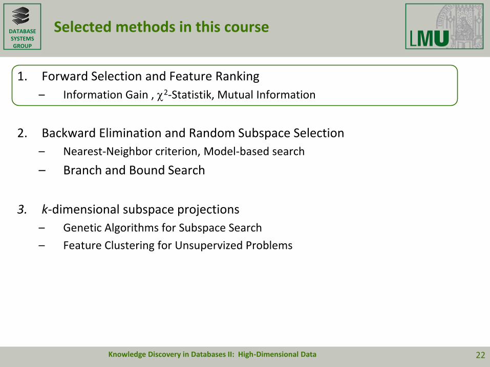
1. Forward Selection and Feature Ranking
– Information Gain , 2-Statistik, Mutual Information
2. Backward Elimination and Random Subspace Selection
– Nearest-Neighbor criterion, Model-based search
– Branch and Bound Search
3. k-dimensional subspace projections
– Genetic Algorithms for Subspace Search
– Feature Clustering for Unsupervized Problems
Knowledge Discovery in Databases II: High-Dimensional Data 22

DATABASESYSTEMSGROUP
1. Forward Selection and Feature Ranking
Input: A supervised learning task
– Target variable C
– Training set of labeled feature vectors <d1, d2, …, dn>
Approach
• Compute the quality q(di ,C) for each dimension di {d1,,..,dn} to predict the correlation to C
• Sort the dimensions d1,,..,dn w.r.t. q(di ,C)
• Select the k-best dimensions
Assumption:
Features are only correlated via their connection to C
=> it is sufficient to evaluate the connection between each single feature d and the target variable C
Knowledge Discovery in Databases II: High-Dimensional Data 23

DATABASESYSTEMSGROUP
Statistical quality measures for features
How suitable is feature d for predicting the value of class attribute C?
Statistical measures :
• Rely on distributions over feature values and target values.
– For discrete values: determine probabilities for all value pairs.
– For real valued features: • Discretize the value space (reduction to the case above)
• Use probability density functions (e.g. uniform, Gaussian,..)
• How strong is the correlation between both value distributions?
• How good does splitting the values in the feature space separate values in the target dimension?
• Example quality measures:– Information Gain
– Chi-square χ2-statistics
– Mutual Information
Knowledge Discovery in Databases II: High-Dimensional Data 24
DATABASESYSTEMSGROUP
Information Gain 1/2
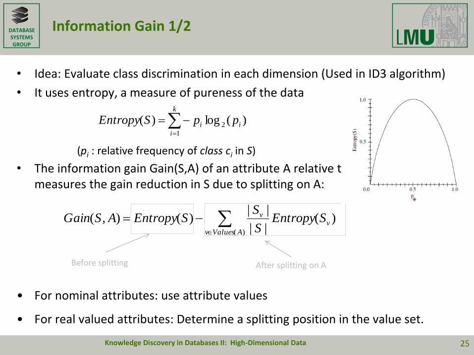
• Idea: Evaluate class discrimination in each dimension (Used in ID3 algorithm)
• It uses entropy, a measure of pureness of the data
• The information gain Gain(S,A) of an attribute A relative to a training set S measures the gain reduction in S due to splitting on A:
• For nominal attributes: use attribute values
• For real valued attributes: Determine a splitting position in the value set.
Knowledge Discovery in Databases II: High-Dimensional Data 25
)(
)(||
||)(),(
AValuesv
vv SEntropy
S
SSEntropyASGain
Before splitting After splitting on A
(pi : relative frequency of class ci in S)
k
i
ii ppSEntropy1
2 )(log)(
DATABASESYSTEMSGROUP
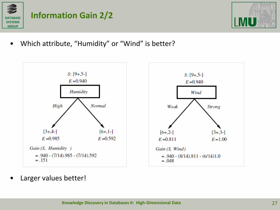
Information Gain 2/2
• Which attribute, “Humidity” or “Wind” is better?
• Larger values better!
Knowledge Discovery in Databases II: High-Dimensional Data 27

DATABASESYSTEMSGROUP
Chi-square χ2 statistics 1/2
• Idea: Measures the independency of a variable from the class variable.
• Contingency table
– Divide data based on a split value s or based on discrete values
• Example: Liking science fiction movies implies playing chess?
• Chi-square χ2 test
Knowledge Discovery in Databases II: High-Dimensional Data 28
c
i
r
j ij
ijij
e
eo
1 1
2
2)(
oij:observed frequency eij: expected frequency n
hhe
ji
ij
Play chess Not play chess Sum (row)
Like science fiction 250 200 450
Not like science fiction 50 1000 1050
Sum(col.) 300 1200 1500
Class attribute
Pre
dic
tor
attr
ibu
te
DATABASESYSTEMSGROUP
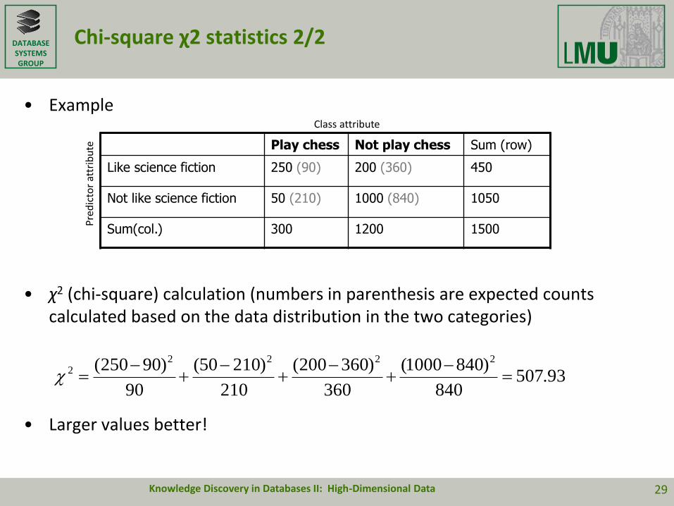
Chi-square χ2 statistics 2/2
• Example
• χ2 (chi-square) calculation (numbers in parenthesis are expected counts calculated based on the data distribution in the two categories)
• Larger values better!
Knowledge Discovery in Databases II: High-Dimensional Data 29
Play chess Not play chess Sum (row)
Like science fiction 250 (90) 200 (360) 450
Not like science fiction 50 (210) 1000 (840) 1050
Sum(col.) 300 1200 1500
Class attribute
Pre
dic
tor
attr
ibu
te
93.507840
)8401000(
360
)360200(
210
)21050(
90
)90250( 22222

DATABASESYSTEMSGROUP
Mutual Information (MI)
Yy Xx ypxp
yxpyxpYXI
)()(
),(log),(),(
Y X
dxdyypxp
yxpyxpYXI
)()(
),(log),(),(
Knowledge Discovery in Databases II: High-Dimensional Data 31
• In general, MI between two variables x, y measures how much knowing one of these variables reduces uncertainty about the other
• In our case, it measures how much information a feature contributes to making the correct classification decision.
• Discrete case:
• Continuous case:
• In case of statistical independence: – p(x,y)= p(x)p(y) log(1)=0– knowing x does not reveal anything about y
p(x,y): the joint probability distribution functionp(x), p(y): the marginal probability distributions
Relation to entropy
DATABASESYSTEMSGROUP
Forward Selection and Feature Ranking -overview
Advantages:• Efficiency: it compares {d1, d2, …, dn} features to the class attribute C instead of
subspaces
• Training suffices with rather small sample sets
Disadvantages: • Independency assumption: Classes and features must display a direct
correlation.
• In case of correlated features: Always selects the features having the strongest direct correlation to the class variable, even if the features are strongly correlated with each other.(features might even have an identical meaning)
Knowledge Discovery in Databases II: High-Dimensional Data
k
n
32

DATABASESYSTEMSGROUP
Selected methods in this course
1. Forward Selection and Feature Ranking
– Information Gain , 2-Statistik, Mutual Information
2. Backward Elimination and Random Subspace Selection
– Nearest-Neighbor criterion, Model-based search
– Branch and Bound Search
3. k-dimensional projections
– Genetic Algorithms for Subspace Search
– Feature Clustering for Unsupervized Problems
Knowledge Discovery in Databases II: High-Dimensional Data 33

DATABASESYSTEMSGROUP
2. Backward Elimination
Idea: Start with the complete feature space and delete redundant features
Approach: Greedy Backward Elimination
1. Generate the subspaces R of the feature space F
2. Evaluate subspaces R with the quality measure q(R)
3. Select the best subspace R* w.r.t. q(R)
4. If R* has the wanted dimensionality, terminate
else start backward elimination on R*.
Applications:
• Useful in supervised and unsupervised setting– in unsupervised cases, q(R) measures structural characteristics
• Greedy search if there is no monotonicity on q(R)=> for monotonous q(R) employ branch and bound search
Knowledge Discovery in Databases II: High-Dimensional Data 34
DATABASESYSTEMSGROUP
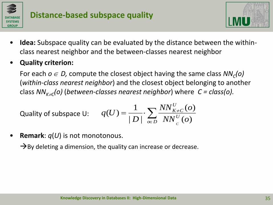
Distance-based subspace quality
• Idea: Subspace quality can be evaluated by the distance between the within-class nearest neighbor and the between-classes nearest neighbor
• Quality criterion:
For each o D, compute the closest object having the same class NNC(o) (within-class nearest neighbor) and the closest object belonging to another class NNKC(o) (between-classes nearest neighbor) where C = class(o).
Quality of subspace U:
• Remark: q(U) is not monotonous.
By deleting a dimension, the quality can increase or decrease.
Do
U
U
CK
oNN
oNN
DUq
C)(
)(
||
1)(
Knowledge Discovery in Databases II: High-Dimensional Data 35
DATABASESYSTEMSGROUP
Model-based approach
• Idea: Directly employ the data mining algorithm to evaluate the subspace.
• Example: Evaluate each subspace by training a Naive Bayes classifier
Practical aspects:
• Success of the data mining algorithm must be measurable
(e.g. class accuracy)
• Runtime for training and applying the classifier should be low
• The classifier parameterization should not be of great importance
• Test set should have a moderate number of instances
Knowledge Discovery in Databases II: High-Dimensional Data 36
DATABASESYSTEMSGROUP
Backward Elimination - overview
Advantages:• Considers complete subspaces (multiple dependencies are used)
• Can recognize and eliminate redundant features
Disadvantages:• Tests w.r.t. subspace quality usually requires much more effort
• All solutions employ heuristic greedy search which do not necessarily find the optimal feature space.
Knowledge Discovery in Databases II: High-Dimensional Data 37
DATABASESYSTEMSGROUP
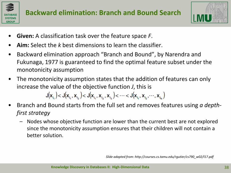
Backward elimination: Branch and Bound Search
Knowledge Discovery in Databases II: High-Dimensional Data 38
• Given: A classification task over the feature space F.
• Aim: Select the k best dimensions to learn the classifier.
• Backward elimination approach “Branch and Bound”, by Narendra and Fukunaga, 1977 is guaranteed to find the optimal feature subset under the monotonicity assumption
• The monotonicity assumption states that the addition of features can only increase the value of the objective function J, this is
• Branch and Bound starts from the full set and removes features using a depth-first strategy
– Nodes whose objective function are lower than the current best are not explored since the monotonicity assumption ensures that their children will not contain a better solution.
Slide adapted from: http://courses.cs.tamu.edu/rgutier/cs790_w02/l17.pdf
DATABASESYSTEMSGROUP
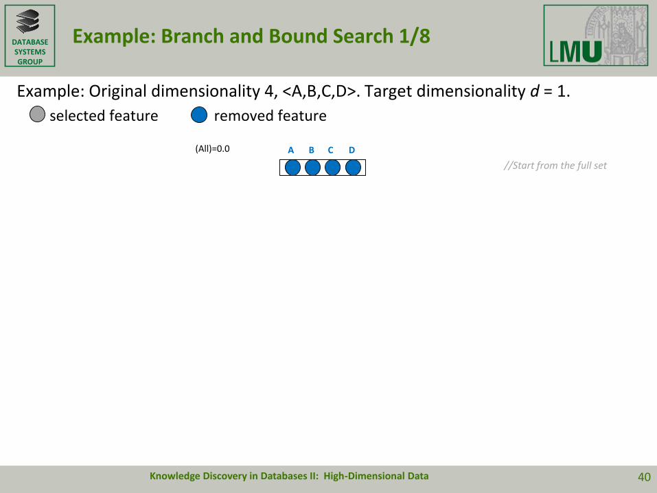
Example: Branch and Bound Search 1/8
Example: Original dimensionality 4, <A,B,C,D>. Target dimensionality d = 1.
selected feature removed feature
(All)=0.0
Knowledge Discovery in Databases II: High-Dimensional Data 40
A B C D
//Start from the full set

DATABASESYSTEMSGROUP
Example: Branch and Bound Search 2/8
Example: Original dimensionality 4, <A,B,C,D>. Target dimensionality d = 1.
selected feature removed feature
(All)=0.0
Knowledge Discovery in Databases II: High-Dimensional Data 41
A B C D
//Generate subspaces
IC (BCD)=0.0IC(ACD)=0.015 IC(ABD)=0.021 IC(ABC)=0.03
DATABASESYSTEMSGROUP
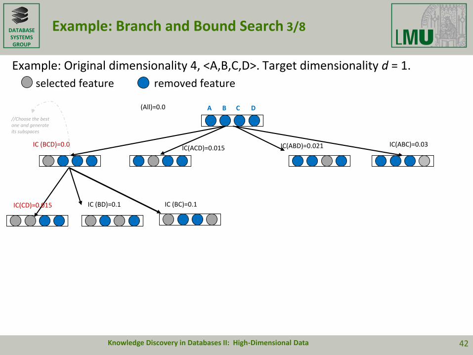
Example: Branch and Bound Search 3/8
Example: Original dimensionality 4, <A,B,C,D>. Target dimensionality d = 1.
selected feature removed feature
(All)=0.0
Knowledge Discovery in Databases II: High-Dimensional Data 42
A B C D
//Choose the best one and generate its subspaces
IC (BCD)=0.0IC(ACD)=0.015 IC(ABD)=0.021 IC(ABC)=0.03
IC(CD)=0.015 IC (BC)=0.1IC (BD)=0.1

DATABASESYSTEMSGROUP
Example: Branch and Bound Search 4/8
Example: Original dimensionality 4, <A,B,C,D>. Target dimensionality d = 1.
selected feature removed feature
(All)=0.0
Knowledge Discovery in Databases II: High-Dimensional Data 43
A B C D
//Choose the best one and generate its subspaces
IC (BCD)=0.0IC(ACD)=0.015 IC(ABD)=0.021 IC(ABC)=0.03
IC(CD)=0.015 IC (BC)=0.1IC (BD)=0.1
IC(D)=0.02 IC(C)=0.03
aktBound = 0.02
//Desired dimensionality reached, what is the bound?
DATABASESYSTEMSGROUP
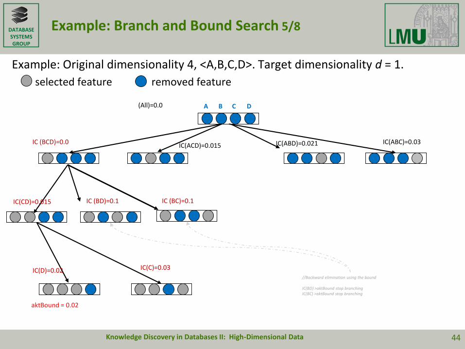
Example: Branch and Bound Search 5/8
Example: Original dimensionality 4, <A,B,C,D>. Target dimensionality d = 1.
selected feature removed feature
(All)=0.0
Knowledge Discovery in Databases II: High-Dimensional Data 44
A B C D
IC (BCD)=0.0IC(ACD)=0.015 IC(ABD)=0.021 IC(ABC)=0.03
IC(CD)=0.015 IC (BC)=0.1IC (BD)=0.1
IC(D)=0.02 IC(C)=0.03
aktBound = 0.02
//Backward elimination using the bound
IC(BD) >aktBound stop branchingIC(BC) >aktBound stop branching

DATABASESYSTEMSGROUP
Example: Branch and Bound Search 6/8
Example: Original dimensionality 4, <A,B,C,D>. Target dimensionality d = 1.
selected feature removed feature
(All)=0.0
Knowledge Discovery in Databases II: High-Dimensional Data 45
A B C D
IC (BCD)=0.0IC(ACD)=0.015 IC(ABD)=0.021 IC(ABC)=0.03
IC(CD)=0.015 IC (BC)=0.1IC (BD)=0.1
IC(D)=0.02 IC(C)=0.03
aktBound = 0.02
//Backward elimination using the bound
IC(ACD) <aktBound do branchingIC(AD)>aktBound stop branchingIC(AC)>aktBound stop branching
IC(AC)=0.03IC (AD)=0.1
DATABASESYSTEMSGROUP
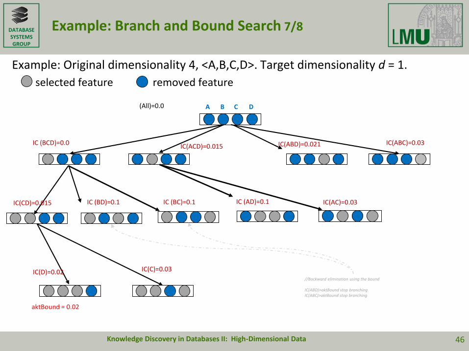
Example: Branch and Bound Search 7/8
Example: Original dimensionality 4, <A,B,C,D>. Target dimensionality d = 1.
selected feature removed feature
(All)=0.0
Knowledge Discovery in Databases II: High-Dimensional Data 46
A B C D
IC (BCD)=0.0IC(ACD)=0.015 IC(ABD)=0.021 IC(ABC)=0.03
IC(CD)=0.015 IC (BC)=0.1IC (BD)=0.1
IC(D)=0.02 IC(C)=0.03
aktBound = 0.02
//Backward elimination using the bound
IC(ABD)>aktBound stop branchingIC(ABC)>aktBound stop branching
IC(AC)=0.03IC (AD)=0.1

DATABASESYSTEMSGROUP
Backward elimination: Branch and Bound Search
Given: A classification task over the feature space F.
Aim: Select the k best dimensions to learn the classifier.
Backward-Elimination based in Branch and Bound:
FUNCTION BranchAndBound(Featurespace F, int k)
queue.init(ASCENDING);
queue.add(F, quality(F))
curBound:= INFINITY;
WHILE queue.NotEmpty() and aktBound > queue.top() DO
curSubSpace:= queue.top();
FOR ALL Subspaces U of curSubSpace DO
IF U.dimensionality() = k THEN
IF quality(U)< curBound THEN
curBound := quality(U);
BestSubSpace := U;
ELSE
queue.add(U, quality(U));
RETURN BestSubSpace
Knowledge Discovery in Databases II: High-Dimensional Data 48
DATABASESYSTEMSGROUP
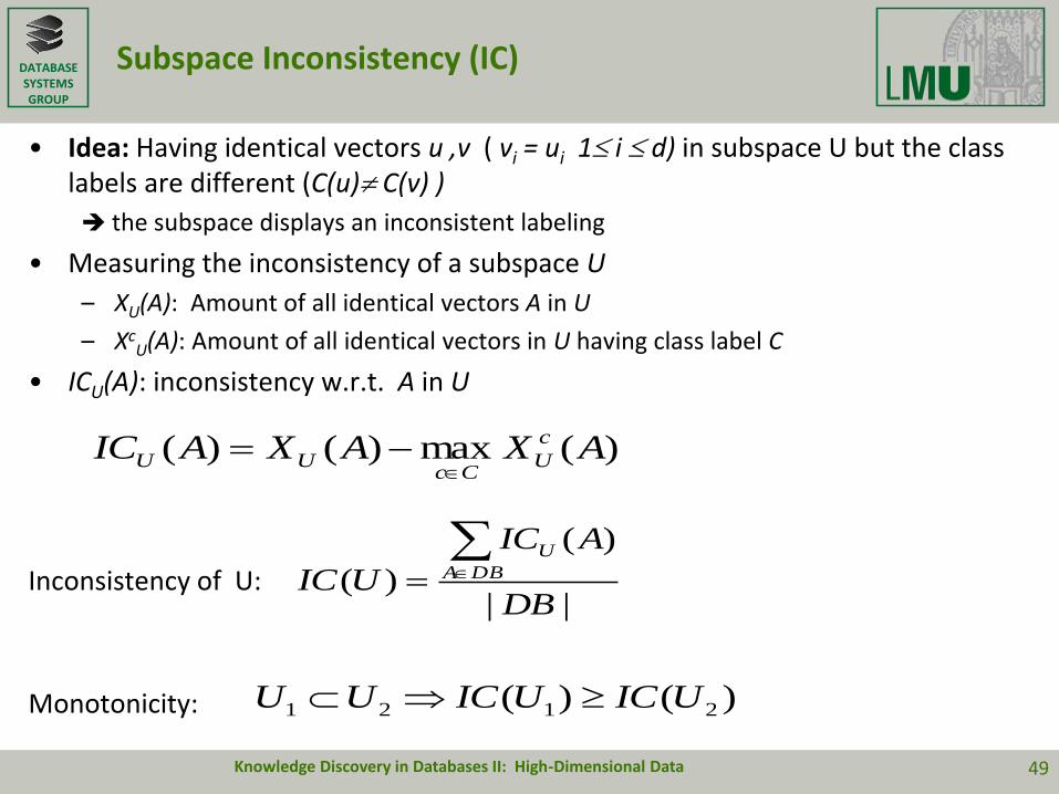
Subspace Inconsistency (IC)
• Idea: Having identical vectors u ,v ( vi = ui 1 i d) in subspace U but the class labels are different (C(u) C(v) )
the subspace displays an inconsistent labeling
• Measuring the inconsistency of a subspace U
– XU(A): Amount of all identical vectors A in U
– XcU(A): Amount of all identical vectors in U having class label C
• ICU(A): inconsistency w.r.t. A in U
Inconsistency of U:
Monotonicity:
)(max)()( AXAXAIC c
UCc
UU
||
)(
)(DB
AIC
UIC DBA
U
)()( 2121 UICUICUU
Knowledge Discovery in Databases II: High-Dimensional Data 49

DATABASESYSTEMSGROUP
Branch and Bound search - overview
Advantage:
• Monotonicity allows efficient search for optimal solutions
• Well-suited for binary or discrete data(identical vectors are very likely with decreasing dimensionality)
Disadvantages:
• Useless without groups of identical features (real-valued vectors)
• Worse-case runtime complexity remains exponential in d
Knowledge Discovery in Databases II: High-Dimensional Data 50

DATABASESYSTEMSGROUP
Selected methods in this course
1. Forward Selection and Feature Ranking
– Information Gain , 2-Statistik, Mutual Information
2. Backward Elimination and Random Subspace Selection
– Nearest-Neighbor criterion, Model-based search
– Branch and Bound Search
3. k-dimensional projections
– Genetic Algorithms for Subspace Search
– Feature Clustering for Unsupervised Problems
Knowledge Discovery in Databases II: High-Dimensional Data 51
DATABASESYSTEMSGROUP
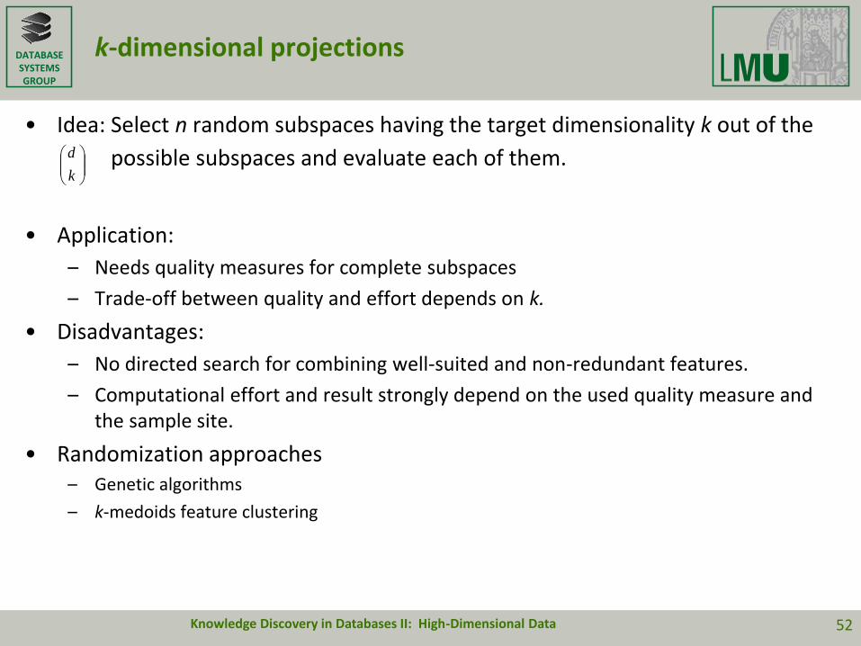
k-dimensional projections
• Idea: Select n random subspaces having the target dimensionality k out of the
possible subspaces and evaluate each of them.
• Application:
– Needs quality measures for complete subspaces
– Trade-off between quality and effort depends on k.
• Disadvantages:
– No directed search for combining well-suited and non-redundant features.
– Computational effort and result strongly depend on the used quality measure and the sample site.
• Randomization approaches– Genetic algorithms
– k-medoids feature clustering
Knowledge Discovery in Databases II: High-Dimensional Data
k
d
52

DATABASESYSTEMSGROUP
Genetic Algorithms
• Idea: Randomized search through genetic algorithms
Genetic Algorithms:
• Encoding of the individual states in the search space: bit-strings
• Population of solutions := set of k-dimensional subspaces
• Fitness function: quality measure for a subspace
• Operators on the population:
– Mutation: dimension di in subspace U is replaced by dimension dj with a likelihood of x%
– Crossover: combine two subspaces U1, U2
o Unite the features sets of U1 and U2.
o Delete random dimensions until dimensionality is k
• Selection for next population: All subspaces having at least a quality of y% of the best fitness in the current generation are copied to the next generation.
• Free tickets: Additionally each subspace is copied to the next generation with a probability of u% into the next generation.
Knowledge Discovery in Databases II: High-Dimensional Data 53

DATABASESYSTEMSGROUP
Genetic Algorithm: Schema
Generate initial population
WHILE Max_Fitness > Old_Fitness DO
Mutate current population
WHILE nextGeneration < PopulationSize DO
Generate new candidate from pairs of old subspaces
IF K has a free ticket or K is fit enough THEN
copy K to the next generation
RETURN fittest subspace
Knowledge Discovery in Databases II: High-Dimensional Data 54

DATABASESYSTEMSGROUP
Genetic Algorithms
Remarks:
• Here: only basic algorithmic scheme (multiple variants)
• Efficient convergence by “Simulated Annealing”
(Likelihood of free tickets decreases with the iterations)
Advantages:
• Can escape from local extreme values during the search
• Often good approximations for optimal solutions
Disadvantages:
• Runtime is not bounded can become rather inefficient
• Configuration depends on many parameters which have to be tuned to achieve good quality results in efficient time
Knowledge Discovery in Databases II: High-Dimensional Data 55
DATABASESYSTEMSGROUP
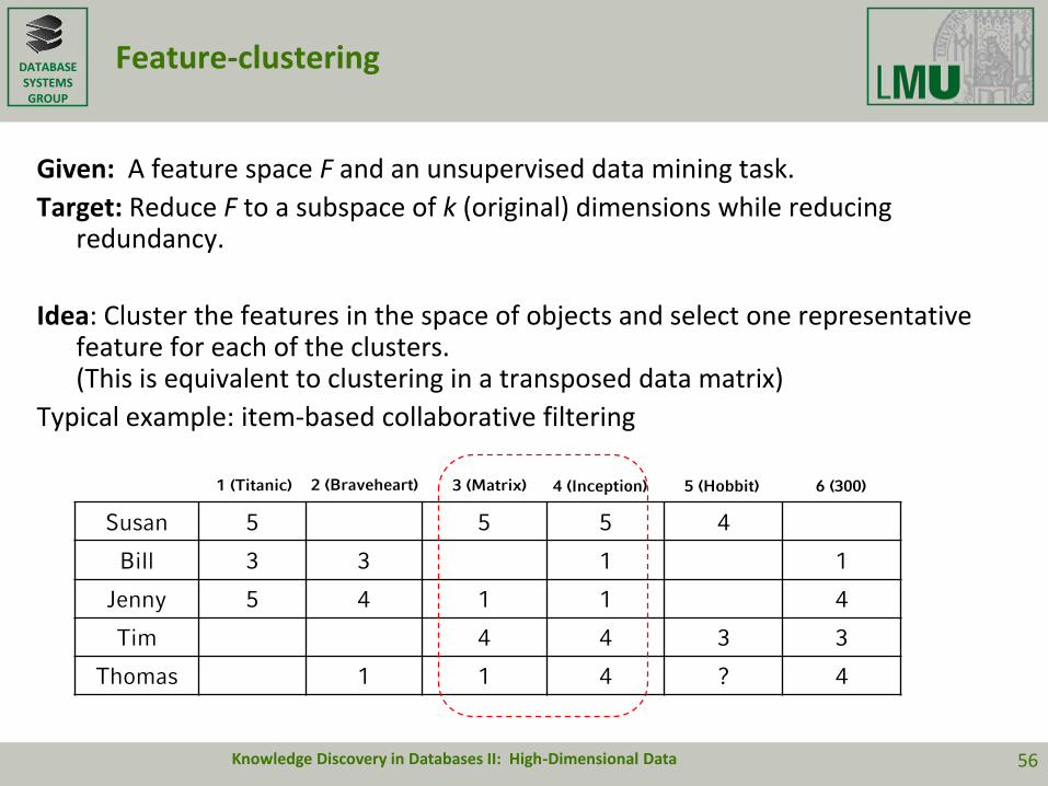
Feature-clustering
Given: A feature space F and an unsupervised data mining task.
Target: Reduce F to a subspace of k (original) dimensions while reducing redundancy.
Idea: Cluster the features in the space of objects and select one representative feature for each of the clusters.(This is equivalent to clustering in a transposed data matrix)
Typical example: item-based collaborative filtering
Knowledge Discovery in Databases II: High-Dimensional Data 56
Susan 5 5 5 4
Bill 3 3 1 1
Jenny 5 4 1 1 4
Tim 4 4 3 3
Thomas 1 1 4 ? 4
1 (Titanic) 2 (Braveheart) 3 (Matrix) 4 (Inception) 5 (Hobbit) 6 (300)
DATABASESYSTEMSGROUP
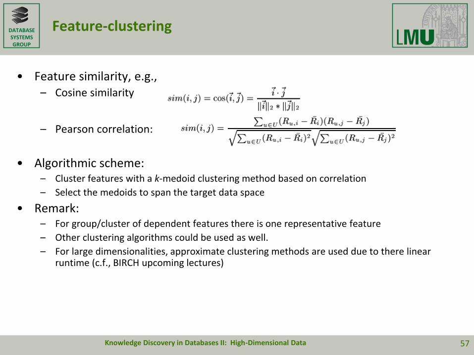
Feature-clustering
• Feature similarity, e.g.,– Cosine similarity
– Pearson correlation:
• Algorithmic scheme: – Cluster features with a k-medoid clustering method based on correlation
– Select the medoids to span the target data space
• Remark: – For group/cluster of dependent features there is one representative feature
– Other clustering algorithms could be used as well.
– For large dimensionalities, approximate clustering methods are used due to there linear runtime (c.f., BIRCH upcoming lectures)
Knowledge Discovery in Databases II: High-Dimensional Data 57

DATABASESYSTEMSGROUP
Feature-Clustering based on correlation
Advantages:
• Depending on the clustering algorithm quite efficient
• Unsupervised method
Disadvantages:
• Results are usually not deterministic (partitioning clustering)
• Representatives are usually unstable for different clustering methods and parameters.
• Based on pairwise correlation and dependencies
=> multiple dependencies are not considered
Knowledge Discovery in Databases II: High-Dimensional Data 58

DATABASESYSTEMSGROUP
Feature selection: overview
• Forward-Selection: Examines each dimension D‘ {D1,,..,Dd}. and selects the k-best to span the target space.
– Greedy Selection based on Information Gain, 2 Statistics or Mutual Information
• Backward-Elimination: Start with the complete feature space and successively remove the worst dimensions.
– Greedy Elimination with model-based and nearest-neighbor based approaches
– Branch and Bound Search based on inconsistency
• k-dimensional Projections: Directly search in the set of k-dimensional subspaces for the best suited
– Genetic algorithms (quality measures as with backward elimination)
– Feature clustering based on correlation
Knowledge Discovery in Databases II: High-Dimensional Data 59
DATABASESYSTEMSGROUP
Feature selection: discussion
• Many algorithms based on different heuristics
• There are two reason to delete features:
– Redundancy: Features can be expressed by other features.
– Missing correlation to the target variable
• Often even approximate results are capable of increasing efficiency and quality in a data mining tasks
• Caution: Selected features need not have a causal connection to the target variable, but both observation might depend on the same mechanisms in the data space (hidden variables).
• Different indicators to consider in the comparison of before and after selection performance
– Model performance, time, dimensionality, …
Knowledge Discovery in Databases II: High-Dimensional Data 60
DATABASESYSTEMSGROUP
What you should know by now
• Reasons for using feature selection
• Curse of dimensionality
• Forward selection and feature ranking
– Information Gain
– 2 Statistics
– Mutual Information
• Backward Elimination
– Model-based subspace quality
– Nearest neighbor-based subspace quality
– Inconsistency and Branch & Bound search
• k-dimensional projections
– Genetic algorithms
– Feature clustering
Knowledge Discovery in Databases II: High-Dimensional Data 61

DATABASESYSTEMSGROUP
Literature
• I. Guyon, A. Elisseeff: An Introduction to Variable and Feature Selection, Journal of Machine Learning Research 3, 2003.
• H. Liu and H. Motoda, Computations methods of feature selection, Chapman & Hall/ CRC, 2008.
• A.Blum and P. Langley: Selection of Relevant Features and Examples in Machine Learning, Artificial Intelligence (97),1997.
• H. Liu and L. Yu: Feature Selection for Data Mining (WWW), 2002.
• L.C. Molina, L. Belanche, Â. Nebot: Feature Selection Algorithms: A Survey and Experimental Evaluations, ICDM 2002, Maebashi City, Japan.
• P. Mitra, C.A. Murthy and S.K. Pal: Unsupervised Feature Selection using Feature Similarity, IEEE Transacitons on pattern analysis and Machicne intelligence, Vol. 24. No. 3, 2004.
• J. Dy, C. Brodley: Feature Selection for Unsupervised Learning, Journal of Machine Learning Research 5, 2004.
• M. Dash, H. Liu, H. Motoda: Consistency Based Feature Selection, 4th Pacific-Asia Conference, PADKK 2000, Kyoto, Japan, 2000.
Knowledge Discovery in Databases II: High-Dimensional Data 62