interoperability and integration of processes of knowledge ...dgorea/thesis.pdf · the knowledge...
TRANSCRIPT

Interoperability and Integration
of Processes of Knowledge
Discovery in Databases
Diana Gorea
Department of Computer Science
University Alexandru Ioan Cuza Iasi
Scientific coordinator: prof. Toader Jucan, PhD
The 16th of January, 2009

I would like to dedicate this thesis to my family.

Acknowledgements
I would like to acknowledge the support offered by my professors.
Abstract
In the context of interoperability in knowledge discovery in databases,
this thesis proposes an architecture of an online scoring system (De-
Visa) that can be integrated easily in loosely coupled service oriented
architectures. It manages a repository of PMML models as a native
XML database and exploits their predictive or descriptive properties.
This thesis proposes a novel technique for online scoring based on web
services and the specification of a specialized XML-based query lan-
guage for PMML models called PMQL, used to enable communication
with the data mining consumers and for processing the models in the
repository. At the abstract level, the thesis presents an theoretical
foundation that captures both structural and behavioral aspects of
the system providing solutions to problems that arise. The structural
aspects includes the mining models/schemas, the data dictionaries
etc. The behavioral aspects include the way the system interacts
with consumers requests, namely scoring or composition requests. A
theoretical framework for allowing prediction model composition is
provided. Among others it uses the concept of semantic consequence
in the functional dependencies theory. In the context of online scor-
ing a novel hybrid technique for schema matching is provided. The
technique is based on a modified version of the cycle canceling max-
flow min-cost algorithm that allows integrating additional constraints
such as derivability and validity. It also proposes an adaptive simi-
larity measure based on string metrics, Jaccard index in the textual
description, field statistics and lexical sense. In this context the work
presents the global data dictionary architecture that alleviates the
overhead of matching complexity within the scoring process and an
algorithm for offline incremental update of the GDD.

Contents
Nomenclature xi
1 Introduction 1
2 Knowledge Discovery in Databases 6
2.1 General Presentation . . . . . . . . . . . . . . . . . . . . . . . . . 6
2.2 Knowledge Discovery Process Models . . . . . . . . . . . . . . . . 7
2.2.1 Academic Models . . . . . . . . . . . . . . . . . . . . . . . 8
2.2.2 Industrial Models . . . . . . . . . . . . . . . . . . . . . . . 9
2.2.3 Hybrid Models . . . . . . . . . . . . . . . . . . . . . . . . 10
2.3 Overview of the Methods for Constructing Predictive Models . . . 10
2.3.1 Unsupervised Learning . . . . . . . . . . . . . . . . . . . . 10
2.3.1.1 Clustering . . . . . . . . . . . . . . . . . . . . . . 10
2.3.1.2 Association Rules . . . . . . . . . . . . . . . . . . 12
2.3.2 Supervised Learning . . . . . . . . . . . . . . . . . . . . . 14
2.3.2.1 Decision Trees . . . . . . . . . . . . . . . . . . . 14
2.3.2.2 Rule Algorithms . . . . . . . . . . . . . . . . . . 16
2.3.3 Model Assessment and other Efficiency Considerations . . 17
2.4 Representing Knowledge within the KDD . . . . . . . . . . . . . . 18
2.4.1 Categories of Knowledge Representation . . . . . . . . . . 19
2.4.1.1 Rules . . . . . . . . . . . . . . . . . . . . . . . . 19
2.4.1.2 Graphs, Trees and Networks . . . . . . . . . . . . 21
2.4.1.3 Predictive Models . . . . . . . . . . . . . . . . . 22
2.5 Interoperability in KDD . . . . . . . . . . . . . . . . . . . . . . . 22
2.5.1 Predictive Model Markup Language . . . . . . . . . . . . . 22
iv

CONTENTS
2.5.1.1 Data Dictionary . . . . . . . . . . . . . . . . . . 24
2.5.1.2 Mining Model . . . . . . . . . . . . . . . . . . . . 25
2.5.1.3 Transformation Dictionary . . . . . . . . . . . . . 26
2.5.1.4 Model Statistics . . . . . . . . . . . . . . . . . . 27
2.5.1.5 PMML Support in Predictive Analysis Products . 28
3 Knowledge as a Service 30
3.1 DeVisa- Architectural Overview . . . . . . . . . . . . . . . . . . . 30
3.1.1 Functional Perspective . . . . . . . . . . . . . . . . . . . . 30
3.2 The Main Components . . . . . . . . . . . . . . . . . . . . . . . . 33
3.3 PMQL - A PMML Query Language . . . . . . . . . . . . . . . . . 39
3.3.1 The Structure of a PMQL Goal . . . . . . . . . . . . . . . 41
3.3.2 PMQL Query Processing . . . . . . . . . . . . . . . . . . . 43
3.3.2.1 Annotation . . . . . . . . . . . . . . . . . . . . . 43
3.3.2.2 Rewriting . . . . . . . . . . . . . . . . . . . . . . 44
3.3.2.3 Plan Building . . . . . . . . . . . . . . . . . . . . 46
3.3.2.4 Plan Execution . . . . . . . . . . . . . . . . . . . 46
3.4 Predictive Models Composition . . . . . . . . . . . . . . . . . . . 47
3.4.1 Methods and Challenges In Composing Data Mining models 47
3.4.2 Model Composition in PMML . . . . . . . . . . . . . . . . 49
3.4.2.1 Model sequencing . . . . . . . . . . . . . . . . . . 49
3.4.2.2 Model selection . . . . . . . . . . . . . . . . . . . 49
3.4.3 Model Composition in DeVisa . . . . . . . . . . . . . . . . 50
3.4.3.1 Implicit Composition . . . . . . . . . . . . . . . . 51
3.4.3.2 Explicit Composition . . . . . . . . . . . . . . . . 51
4 DeVisa - Formal Model 52
4.1 Overview of DeVisa Concepts . . . . . . . . . . . . . . . . . . . . 52
4.1.1 The connection between the mining models and functional
dependencies . . . . . . . . . . . . . . . . . . . . . . . . . 55
4.2 The Scoring Process . . . . . . . . . . . . . . . . . . . . . . . . . 58
4.2.1 Model Discovery . . . . . . . . . . . . . . . . . . . . . . . 59
4.2.1.1 Exact Model or Exact Schema Case . . . . . . . 59
4.2.1.2 Match Schema Case . . . . . . . . . . . . . . . . 60
v

CONTENTS
4.2.2 Scoring . . . . . . . . . . . . . . . . . . . . . . . . . . . . . 66
4.3 The Composition Process . . . . . . . . . . . . . . . . . . . . . . 66
4.3.1 Implicit composition . . . . . . . . . . . . . . . . . . . . . 66
4.3.1.1 Late Composition . . . . . . . . . . . . . . . . . 68
4.3.1.2 Structural Composition . . . . . . . . . . . . . . 68
4.3.2 Explicit Composition . . . . . . . . . . . . . . . . . . . . . 72
5 Semantic Integration and the Implications in DeVisa 74
5.1 Basic Terminology . . . . . . . . . . . . . . . . . . . . . . . . . . 74
5.2 Applications of Semantic Integration . . . . . . . . . . . . . . . . 76
5.3 Strategies in Achieving Schema and Ontology Mapping . . . . . . 78
5.3.1 Overview of the Existing Approaches . . . . . . . . . . . . 81
5.4 Implications of the Schema Mapping in DeVisa . . . . . . . . . . 86
5.5 Schema Matching Approach in DeVisa . . . . . . . . . . . . . . . 89
5.5.1 The Validation of the Matching . . . . . . . . . . . . . . . 108
5.6 The Similarity Measure . . . . . . . . . . . . . . . . . . . . . . . . 108
6 Related Work 117
6.1 Online Scoring and Online Data Mining Services . . . . . . . . . . 117
6.2 PMML Scoring Engines . . . . . . . . . . . . . . . . . . . . . . . 119
6.2.1 Augustus . . . . . . . . . . . . . . . . . . . . . . . . . . . 119
6.3 Comparison to DeVisa’s approach . . . . . . . . . . . . . . . . . . 121
7 Implementation Details 123
7.1 Overview of the Underlying Technologies . . . . . . . . . . . . . . 123
7.1.1 Native XML Database Systems . . . . . . . . . . . . . . . 123
7.1.2 XQuery . . . . . . . . . . . . . . . . . . . . . . . . . . . . 124
7.1.3 eXist . . . . . . . . . . . . . . . . . . . . . . . . . . . . . . 124
7.1.4 Web Services . . . . . . . . . . . . . . . . . . . . . . . . . 125
7.2 Current DeVisa Implementation . . . . . . . . . . . . . . . . . . . 126
vi

CONTENTS
8 Applications 128
8.1 DeVisa in a SOA . . . . . . . . . . . . . . . . . . . . . . . . . . . 128
8.2 DeVisa as a Knowledge Repository for Learning Interface Agents 130
8.3 Application of DeVisa in the microRNA discovery problem . . . . 132
8.4 Other Applications . . . . . . . . . . . . . . . . . . . . . . . . . . 132
8.5 A Concrete Use Case . . . . . . . . . . . . . . . . . . . . . . . . 134
8.5.1 Description of the Data Sets . . . . . . . . . . . . . . . . . 135
8.5.2 The Front End . . . . . . . . . . . . . . . . . . . . . . . . 137
8.5.3 Methods and Results . . . . . . . . . . . . . . . . . . . . . 138
8.5.3.1 Model Selection Use Case . . . . . . . . . . . . . 139
8.5.3.2 Schema Match with Global Data Dictionary Use
Case . . . . . . . . . . . . . . . . . . . . . . . . . 146
9 Conclusions and Further Work 149
9.1 The Contributions of this Work . . . . . . . . . . . . . . . . . . . 149
9.2 Further Research Dirrections . . . . . . . . . . . . . . . . . . . . . 153
A PMQL Specification 155
B Catalog Schema 164
C Use Cases 170
D List of Acronyms 174
References 191
vii

List of Figures
2.1 The six-step hybrid model (Cios & Kurgan (2005)). . . . . . . . . 11
3.1 The DeVisa main functional blocks. . . . . . . . . . . . . . . . . . 31
3.2 The architecture of DeVisa. . . . . . . . . . . . . . . . . . . . . . 34
3.3 The Concepts and Relations that are modeled by the Metadata
Catalog. . . . . . . . . . . . . . . . . . . . . . . . . . . . . . . . . 35
3.4 The Global Data Dictionary as a mediator over the data dictio-
naries in DeVisa. . . . . . . . . . . . . . . . . . . . . . . . . . . . 36
3.5 An example of matching between the Global Data Dictionary and
the individual data dictionaries. Within a data dictionary mining
schemas can overlap. For instance, in DD1, field C is part of
two mining schemas. The field matches are annotated with the
confidence factor. A field can match only one entry in the GDD
with confidence factor 1. . . . . . . . . . . . . . . . . . . . . . . . 37
3.6 Resolving consumers’ goals in DeVisa. . . . . . . . . . . . . . . . 41
3.7 The internal mechanism of the PMQL engine. . . . . . . . . . . . 44
4.1 An example of late composition of models. The comb function
applies a voting procedure or an average on the outcomes of the
individual models. . . . . . . . . . . . . . . . . . . . . . . . . . . . 69
4.2 An example of implicit sequencing of models. . . . . . . . . . . . 69
4.3 Explicit composition of models in DeVisa through a stacking ap-
proach. . . . . . . . . . . . . . . . . . . . . . . . . . . . . . . . . 73
5.1 A taxonomy of the dimensions that characterize the schema/ontology
matching strategies (Rahm & Bernstein (2001)). . . . . . . . . . . 82
viii
LIST OF FIGURES
5.2 An example of a valid matching using tripartite graph representa-
tion. The set of bold paths represents a valid local match function.
The two data dictionaries are represented in squares and diamonds
respectively. . . . . . . . . . . . . . . . . . . . . . . . . . . . . . . 91
5.3 Examples of match functions (b) and the corresponding flow-network
conform to algorithm 5.5.3 (a). The match function µ3 has maxi-
mum confidence and will be chosen. . . . . . . . . . . . . . . . . . 99
5.4 The sequence of max-flows and their corresponding residual net-
works. The negative cost cycles and augmenting paths are depicted
in bold. . . . . . . . . . . . . . . . . . . . . . . . . . . . . . . . . 107
8.1 The General SOA Architecture. . . . . . . . . . . . . . . . . . . . 129
8.2 Integration of DeVisa in a SOA architecture. . . . . . . . . . . . . 130
8.3 The consumer’s metadata and univariate statistics for numeric fields.140
8.4 A subset of the Hungarian metadata on which the J48 decision
tree model (DeVisa ID 21) is defined and the univariate statistics
for the numeric fields. . . . . . . . . . . . . . . . . . . . . . . . . . 141
8.5 A subset of the Long Beach metadata on which the MLP model
(DeVisa ID 10) is defined and the univariate statistics for the nu-
meric fields. . . . . . . . . . . . . . . . . . . . . . . . . . . . . . . 141
8.6 A subset of the Cleveland metadata on which the Logistic Regres-
sion model (DeVisa ID 15) is defined and the univariate statistics
for the numeric fields. . . . . . . . . . . . . . . . . . . . . . . . . . 142
8.7 The accuracy, true positive rate, false positive rate and the area
under the ROC curve of the three base classifiers measured through
10-fold cross validation. . . . . . . . . . . . . . . . . . . . . . . . . 143
8.8 A PDI workflow representing the scoring using heterogeneous model
selection based on the heart disease data dictionary. . . . . . . . . 143
8.9 The Prediction Voting step dialog. . . . . . . . . . . . . . . . . . 144
8.10 The accuracy, true positive rate and false positive rate of the three
base classifiers, the averages and of DeVisa selection, measured
through testing them with the consumer’s data set. . . . . . . . . 145
ix
LIST OF FIGURES
8.11 The ROC analysis of the predictions on the consumer’s data set of
the three base classifiers and of DeVisa late composition, measured
through thresholding the output probabilities. . . . . . . . . . . . 146
8.12 A PDI workflow representing the schema match over consumer’s
metadata and the global data dictionary during scoring over a
repository of heart-related prediction models. . . . . . . . . . . . . 147
C.1 The scoring use case. . . . . . . . . . . . . . . . . . . . . . . . . 170
C.2 The explicit model composition use case. . . . . . . . . . . . . . 171
C.3 The model search use case. . . . . . . . . . . . . . . . . . . . . . 172
C.4 The object model of the PMQL engine component in DeVisa. . . 173
x

List of Algorithms
3.2.1 The incremental update of the GDD when a new data dictionary
is uploaded in DeVisa . . . . . . . . . . . . . . . . . . . . . . . . . 38
4.3.1 Deciding if a Horn clause is a logical consequence of a set of Horn
clauses. . . . . . . . . . . . . . . . . . . . . . . . . . . . . . . . . . 71
5.5.1 Finding a a valid applicable local matching for the consumer’s
schema. . . . . . . . . . . . . . . . . . . . . . . . . . . . . . . . . 92
5.5.2 Transformation of the DeVisa weighted bipartite graph into a mul-
tiple source single sink flow network. . . . . . . . . . . . . . . . . 96
5.5.3 Applying the max-confidence max-flow algorithm for the individual
data dictionaries and selecting the one that is both derivable and
has maximum confidence. . . . . . . . . . . . . . . . . . . . . . . 98
5.5.4 getMaxF lows(Gif ) . . . . . . . . . . . . . . . . . . . . . . . . . . 101
5.5.5 getNegativeCycle(Gif , t) . . . . . . . . . . . . . . . . . . . . . . . 104
5.5.6 getAugmentingPath(Gif) . . . . . . . . . . . . . . . . . . . . . . 105
5.5.7 getMaxF low(Gif ) . . . . . . . . . . . . . . . . . . . . . . . . . . . 106
xi

Chapter 1
Introduction
The general area of this thesis subscribes to the domain of managing and sharing
the knowledge obtained through knowledge discovery in databases processes. The
knowledge discovery in databases (KDD) is a vast domain, whose purpose is to
extract high-level knowledge from data. It consists of a sequence of steps that
can be roughly divided into understanding the domain, pre-processing the data,
data mining and applying the generated knowledge in the domain.
There has been a lot of effort both in academia and industry to formalize the
KDD processes into a common framework. Among these initiatives we mention
Fayyad et al. (1996a), Cios & Kurgan (2005) and Wirth & Hipp (2000). The
proposed frameworks are in many aspects very similar but differ slightly in the
number of steps, applicability in certain application domains, specific objectives
that are emphasized etc.
KDD is an expensive exercise in general and therefore limited to a certain
category of organization. Some of the phases are extremely time consuming (e.g
data pre-processing) and the infrastructure to deploy these processes requires high
expertise and most of the times expensive hardware and software. The natural
consequence is that knowledge has a broader purpose beyond its direct use in
the system that has built it. Thus knowledge should be shared and transfered
between different systems.
The use of popular industrial standards based on XML (XML) can add value
along the KDD chain allowing knowledge interchange between applications in
a platform and technology independent manner. During the past several years,
1

the Data Mining Group DMG has been working in this direction specifying the
Predictive Model Mark-up Language or PMML PMML, a standard XML-based
language for interchanging knowledge between applications.
The high-level knowledge that is the outcome of KDD can be represented in
many forms, such as logical rules, decision trees, fuzzy rules, Bayesian belief net-
works, artificial neural networks etc. These are often called models and represent
a relationship between the input and the output data. Most of the models are
supported by the PMML standard.
The most common platform for data mining is a single workstation. More
recently, data mining systems have been developed that use web services and
service oriented architectures. Consequently, systems have been developed that
provide knowledge as a service (Ali et al. (2005)) or even knowledge applications
based on cloud infrastructures (Grossman & Gu (2008)).
Sometimes in practice it can occur that several available models that achieve
more or less the same function and operate on the same concepts are available.
In this situation the user should be offered the possibility of choosing the model
that best suits its needs or even combine the results of the existing models.
The latter approach is called model composition and has often proved to achieve
better predictive performance than the individual models. In general this is not
straightforward because the composition itself is only partially defined, covering
a limited number of use cases. Furthermore, the combined models share the
disadvantage of being difficult to analyze: they can comprise dozens or even
hundreds of individual models, and although they perform well it is not easy
to understand in intuitive terms what factors are contributing to the improved
decisions. On the other side there are several interpretations of the concept of
model composition, which are discussed further in this thesis.
Generally speaking the contribution of this work lies in extending the idea
of reuse and sharing of knowledge obtained through the KDD processes in the
context of KDD globalization. Therefore knowledge can be further stored, ef-
ficiently managed and provided via web services. The work presents a system
called DeVisa (DeVisa) that is based on collecting knowledge in a domain and
further providing it as a service to consumer applications. It is intended to pro-
vide feasible solutions for dynamic knowledge integration into applications that
2

do not necessarily have to deal with knowledge discovery processes. Nowadays
the true value of KDD is not relying on its collection of complex algorithms,
but moreover on the practical problems that the knowledge produced by these
algorithms can solve. Therefore DeVisa focuses on collecting such knowledge and
further providing it as a service in the context of service oriented architectures.
DeVisa provides several services, whose general description was presented in
Gorea (2008a) and Gorea (2008b). The scoring service represents a mean to
provide knowledge as a service in DeVisa. In this context Gorea (2008c) formalizes
the main entities in the system and the online scoring problem. In addition the
work provides a general context in which composition of data mining models can
be achieved within the boundaries of this online scoring system(Gorea (2008d)).
A PMML query language, called PMQL, used both and for interacting with the
consumer is defined.
Early work on this topic presents some general features of the system and
potential uses cases (customer reliability in banking applications, knowledge bases
for interface agents, bioinformatics applications). In Gorea & Felea (2005), Gorea
(2005c) and Gorea & Buraga (2006) the idea of storing decision tree prediction
models and applying online predictions that can be integrated into decentralized
software architectures and in Semantic Web (SW) was depicted. Gorea (2007)
gives a more detailed overview of the system, although the means through which
the models should be processed were still not very clearly specified.
This work is organized as follows.
Chapter 1 provides a general overview of the knowledge discovery in databases,
highlighting the efforts in the academic and industrial communities to unify the
processes in common frameworks. In this context the necessity to interchange
knowledge is concretized through the definition of a standard language named
PMML for expression of high level knowledge obtained via KDD. Therefore the
ability to store and exchange predictive models through the use of the PMML
standard is presented.
Chapter 2 defines the notion of knowledge as a service and positions the
DeVisa system in the field. It gives a functional and architectural perspective
of DeVisa. The functional perspective highlights the main services that De-
Visa exposes - scoring, composition, search, comparison, administration and the
3

mechanisms used in DeVisa for resolving consumer’s goals,. The architectural
perspective focuses on the main internal components - PMQL engine, PMML
repository, metadata catalog - and the interaction between them. A language
called PMQL (specified by DeVisa) designed especially for interaction between
the DM consumers and DeVisa is presented. PMQL allows expressing consumer’s
goals and the answers to the goals. The chapter ends with a highlight on the pro-
cess of composition of prediction models. It first presents an overview of the
existing approaches to model composition and the types of model composition
supported by the PMML standard. Furthermore several possible approaches for
the prediction models composition problem in DeVisa are presented.
Chapter 3 provides the formalization of the main entities DeVisa is composed
of and of the main functionality. More exactly, the data dictionaries, the min-
ing models/schemas, the repository and the metadata catalog are defined using
formalisms from the relational model. Furthermore, some behavioral aspects are
captured, such as the scoring process, matching schemas or composition process.
The mining models/schemas are defined in terms of the functional dependency
theory and a basic framework to derive new models is described. This approach
is used further in the composition process when a new model needs to be derived
from a set of models conforming to schemas in a certain data dictionary.
Chapter 4 is dedicated to the schema integration problem. First different fla-
vors of the problem are overviewed and different strategies to solve the problem
are investigated. Furthermore the chapter presents the projection of the schema
integration problem in DeVisa and defines a new hybrid 1 : 1 schema matching
strategy as well as a new adaptive similarity measure. The schema matching
strategy is partly modeled as the max-confidence min-flow problem and an algo-
rithm is provided. The similarity measure is multi-faceted, being able to adapt
to available schema information.
Chapter 5 presents mostly related work in the field of scoring engines, knowl-
edge as a service and online predictive models interchange in general and high-
lights DeVisa distinguishing features with respect to the existing approaches.
Chapter 6 presents a few implementation details, including an overview of
the technologies that DeVisa is based on. It also presents the currents status of
the implementation, comprising the PMQL specification, the schema matching
4

technique implementation, the PMQL web service, the XQuery scoring functions,
the Weka PMML export etc.
Chapter 7 presents several usage examples of the system, including: integra-
tion in a SOA as a decision support module, in particular in e-Health systems,
integration in Semantic Web context as a knowledge base for agents, or aggre-
gating the existing PMML predictive models that were published in the recent
scientific work in the micro-RNA discovery problem into a common repository
and providing further predictive support or deriving new potentially more pow-
erful models from the existing ones. In addition the chapter presents a concrete
example, built on top of the Pentaho Data Integration (PDI) tool, in which sev-
eral DeVisa functions are developed as plug-ins. The example uses 3 data sets
in the UCI machine learning repository , namely Heart disease, Arrhythmia, and
Echocardiogram. The use cases are modeled as data flows in PDI and present the
model selection (or implicit late composition) and schema matching scenarios.
Chapter 8 presents conclusions to the present work and draws roadmap with
possible research directions or implementation plans.
The first appendix presents the PMQL specification document based on XML
Schema. The second appendix presents the metadata catalog specification that
needs to be implemented by any DeVisa instance. The third appendix presents
the scoring, explicit composition, search and comparison use cases expressed as
sequence diagrams.
Out of all the bibliographical citations a number of 12 represent original con-
tributions of the author (either as unique author or as a co-author). The pub-
lications belong to well known international academic publishing houses. The
current work was partially supported by the CNCSIS contract type PN-TD num-
ber 404/200, director Diana Gorea.
5
Chapter 2
Knowledge Discovery in
Databases
2.1 General Presentation
Knowledge discovery in databases (KDD) is a non-trivial process of identifying
valid, novel, potentially useful, and ultimately understandable patterns in data
(Fayyad et al. (1996b)). The goal is to seek new relevant knowledge about an
application domain.
The domain concerns the entire process of knowledge extraction, including
the way raw data is stored, understood, cleaned, transformed, the analysis and
understanding of the domain, the algorithms that are applied, evaluation of the
results, interpretation of the results, integration of the knowledge back into the
domain etc. Thus the process consists of a sequence of steps, each of the steps
being based upon the successful completion of the previous step.
KDD is a field that has evolved from the intersection of research fields such
as machine learning, pattern recognition, databases, statistics, AI, knowledge
acquisition from expert systems, data visualization and high performance com-
puting. The unifying goal is to obtain high-level knowledge from low-level data.
Knowledge can be represented in many forms, such as logical rules, decision trees,
fuzzy rules, Bayesian belief networks, and artificial neural networks. The data
mining component of KDD relies on techniques from machine learning, pattern
6
2.2 Knowledge Discovery Process Models
recognition or statistics to build patterns or models that are further used to ex-
tract knowledge. Thus data mining applies algorithms that -under acceptable
computational efficiency limitations- produce the patterns or models.
In general, building data mining models is very expensive because it involves
analyzing large amounts of data. It is universally acknowledged that the data
pre-procesing phase is the most consuming step in terms of computational time
(Cios & Kurgan (2005)). Pre-processing the data involves collecting, cleaning,
transforming, preparing the raw data. In the case in which the data resides
in different heterogeneous sources an integration phase adds up to the process,
making it even more expensive. In the modeling phase the complexity of the
algorithms generally depends on various factors like the prior knowledge about the
domain, the size of the schema and the number of data instances. A considerable
focus in the literature has been on the algorithmic aspect of data mining. A
systematic overview and comparative analysis of data mining algorithms as well
as a comprehensive discussion on the computational complexity can be found in
Lim & Shih (2000), Fasulo (1999), Hand et al. (2001) and Ian H. Witten (2005).
2.2 Knowledge Discovery Process Models
The knowledge discovery process can be formalized into a common framework
using process models. A KD process model provides an overview of the life cycle
of a data mining project, containing the corresponding phases of a project, their
respective tasks, and relationships between these tasks. There are different pro-
cess models originating either from academic or industrial environments. All the
processes have in common the fact that they follow a sequence of steps which are
more or less resembling between models. Although the steps are executed in a
predefined order and depend on one another (in the sense that the outcome of a
step can be the input of the next step), it is possible that, after execution of a
step, some previous steps are re-executed taking into consideration the knowledge
gained in the current step (feedback loops).
An interesting issue that arrises in any KDD process model is choosing which
algorithm or method should be used in each phase of the process to get the best
results from a dataset. Since taking the best decision depends on the properties
7

2.2 Knowledge Discovery Process Models
of the datset, Popa et al. (2007) proposes a multi-agent architecture for recom-
mendation and execution of knowledge discovery processes.
2.2.1 Academic Models
The most representative model in this category is the nine step model introduced
in Fayyad et al. (1996a), which consists of the following steps:
1. Understanding the application domain. This step involves learning the prior
knowledge about the domain and about the user’s goals.
2. Creating a target data set. A subset of the initial data needs to be filtered
through means of selection and projection.
3. Data cleaning and preprocessing. This step involves dealing with outliers,
noise and missing values etc.
4. Data reduction and projection. Methods for dimension reduction and trans-
formation are applied in order to find an invariant representation of the
data.
5. Choosing the data mining task. The user’s goals need to be matched against
a known data mining task, such as classification, regression, clustering etc.
6. Choosing the data mining algorithm. The appropriate algorithm for the
task identified in the previous step is chosen and its parameters are adjusted.
7. Data mining. The models or patterns are generated based on the chosen
algorithm.
8. Interpreting mined patterns. This involves visualization of the extracted
knowledge and data visualization based on this knowledge.
9. Consolidating discovered knowledge. This step involves incorporating the
knowledge into the domain, documenting it and reporting it to the user. It
is possible that the new knowledge conflicts with the previously obtained
knowledge. In this case the appropriate measures needs to be taken.
8

2.2 Knowledge Discovery Process Models
2.2.2 Industrial Models
The academic models usually don’t take into consideration the industrial issues.
Therefore in the industrial world some efforts were developed to adapt the KD
process models to their business needs. In this category the most representative
is the CRISP-DM (CRoss Industry Standard Process for Data mining) model,
a tool-neutral process model initially developed by a consortium of companies.
Nowadays the model has strong support in the industrial world. The process
consists of six steps:
1. Business understanding. This step involves understanding the project ob-
jectives and requirements from a business perspective, and then converting
this knowledge into a data mining problem definition.
2. Data understanding. This comprises initial data collection, getting famil-
iar with the data, identifying data quality problems, detecting interesting
subsets to form hypotheses for hidden information.
3. Data preparation. It covers all activities to construct the final dataset (data
that will be fed into the modeling tool). Data preparation tasks are likely
to be performed multiple times, and not in any prescribed order. Tasks
include table, record, and attribute selection as well as transformation and
cleaning of data for modeling tools.
4. Modeling. Various modeling techniques are selected and applied, and their
parameters are calibrated to optimal values. Typically, there are several
techniques for the same data mining problem type. Some techniques have
specific requirements on the form of data. Therefore, stepping back to the
data preparation phase is often needed.
5. Evaluation. It ensures that the obtained knowledge properly achieves the
business objectives. A key objective is to determine if there is some impor-
tant business issue that has not been sufficiently considered. At the end
of this phase, a decision on the use of the data mining results should be
reached.
9

2.3 Overview of the Methods for Constructing Predictive Models
6. Deployment. The knowledge gained will need to be organized and presented
in a way that the customer can use it. This normally can range from
generating reports or implementing a repeatable data mining process.
2.2.3 Hybrid Models
A hybrid model that combines aspects from both worlds is the six step model
presented in Cios & Kurgan (2005). Although it is based on CRISP-DM, it
provides a more general, research-oriented description of the steps and adding
more explicit feedback loops. The model is depicted in figure 2.1
From the perspective of the current work this is the most interesting because
it highlights an extension to the knowledge usage step, in which the knowledge
discovered for a particular domain can be applied to other domains.
A feasible consequence is that some users or organizations, called consumers,
can benefit from the knowledge acquired in a completely different context by the
producers. The consumers do not need to have extensive background knowledge
or manipulate the data. This goal involves storing and exchanging knowledge
together with the metadata associated with the domain.
2.3 Overview of the Methods for Constructing
Predictive Models
2.3.1 Unsupervised Learning
Unsupervised Learning paradigm is a process that automatically reveals structure
in a data set without any supervision.
2.3.1.1 Clustering
Given X = {x1, x2, . . . xm} a set of n-dimensional tuples, the problem is to identify
groups (clusters) of tuples which belong together (are similar). The similarity is
defined in terms of different metrics, depending on the type of the features of
the tuples. For continuous features one can use many distance functions such as
Euclidean, Hamming, Tchebyshev, Minkowsky, Camberra, angular separation.
10

2.3 Overview of the Methods for Constructing Predictive Models
Understanding of the Problem Domain
Understanding of the Data
Preparation of the Data
Data Mining
Evaluation of the Discovered Knowledge
Use of the Discovered Knowledge
Input Data(database, images, video, semi-
structured data, etc.)
Knowledge(patterns, rules, clusters,
classification, associations, etc.)
Extend knowledge to other domains
Figure 2.1: The six-step hybrid model (Cios & Kurgan (2005)).
For binary features one can use similarity coefficients such as Russel, Jaccard or
Czekanowski. There are several approaches to clustering:
1. Hierarchical, in which either clusters are gradually grown by agglomerating
similar instances (bottom up) or are divided as dissimilar instances are
separated (top down). The distance between clusters is calculated through
various methods, as single link, complete link or average link. Hierarchical
11

2.3 Overview of the Methods for Constructing Predictive Models
clustering produces a graphical representation of the data (dendrogram).
2. Partition-based, in which an objective function (performance index) needs to
be minimized. A good choice of the objective function reveals the true struc-
ture of the data. Depending on the formulation of the objective function
and on the organization of the optimization activities, the most representa-
tive approaches are: k-means, growing a hierarchy of clusters, kernel-based
clustering, k-medoids, fuzzy c-means.
3. Model-based, in which a probabilistic model is assumed and its parameters
are estimated.
4. Grid-based, in which cluster structures are described in the language of
generic geometric constructs line hyperboxes and their combinations.
2.3.1.2 Association Rules
Given a set of items I = {i1, . . . im} and a set of transactions D ⊆ 2I , where
each transaction T ∈ D has associated an unique identifier tid. A transaction
contains an itemset A ⊂ I if and only if A ⊆ T . A is a k-itemset if |A| = k.
If A, B ⊂ I, A ∩ B = ∅, we define an association rule as a dependency A ⇒B[support, confidence] (Agrawal & ad A. Swami (1993)).
Support and confidence are used to measure the quality of a given rule in
terms of its usefulness and certainty.
The support indicates the frequency (probability) of the entire rule with re-
spect to D, being defined as the fraction of transactions containing A and B to
the total number of transactions, or the probability of co-occurrence of A and B.
support(A⇒ B) = P (A ∪ B) =|{T ∈ D|A ∪ B ⊆ T}|
|D|
The confidence indicates the strength of implication in the rule and is defined
as the fraction of transactions containing A and B to the number of transactions
containing A.
confidence(A⇒ B) = P (B|A) =|{T ∈ D|A ∪ B ⊆ T}||{T ∈ D|A ⊆ T}|
12

2.3 Overview of the Methods for Constructing Predictive Models
Both measures are often represented in terms of a minimum threshold (let’s
denote them as smin and cmin). Rules that satisfy both minimum thresholds are
called strong association rules. The support count for an itemset A is defined as:
supCount(A) = |{T ∈ D|A ⊆ T}|
A is a frequent itemset if supCount(A) ≥ smin ∗ |D|, where smin ∗ |D| is called
the minimum support count.
To generate single dimensional association rules the following four steps are
used:
1. Prepare input data in transactional format
2. Choose items of interest, i.e itemsets
3. Compute support counts to evaluate whether selected items are frequent,
i.e whether they satisfy minimum support
4. Generate strong association rules that satisfy the minimum confidence by
computing the conditional probabilities.
Depending on the second and third step, there are different approaches de-
pending on the computational complexity:
1. The Naive Algorithm, that explores the entire solution space (2mn itemsets),
which makes it computationally infeasible for a large number of items;
2. The A priori Algorithm, (Agrawal & Srikant (1994)), which uses prior
knowledge about the property that all nonempty subsets of an frequent
itemset must also be frequent.This property is used to reduce the number
of itemsets that must be searched to find frequent itemsets. Improvements
on the a priori algorithm include hashing, removal of transactions, parti-
tioning, sampling or mining itemsets without candidate generation.
13

2.3 Overview of the Methods for Constructing Predictive Models
2.3.2 Supervised Learning
There are three dominant groups in the domain of supervised learning, namely
statistical methods, neural networks and inductive machine learning. Statistical
methods include the Bayesian methods and regression models. The rest of this
section overviews briefly some of the inductive machine learning algorithms.
Inductive machine learning is a technique used to learn from examples. The
central concept is that of an hypothesis, that approximates a concept and is gen-
erated by the given algorithm (learner) based on a given data set. Let us consider
that the training set is S = {(xi ∈ Cj|i = 1, . . . , N, j = 1, . . . , c)}, where x1, . . . xN
are the N -dimensional data instances and C1, . . . , Cc are the classes (categories)
data tuples, which are a priori known. The classes are often represented through
decision attributes. S represents information about a domain.
The hypotheses are expressed as production rules that cover the examples. In
general the algorithm needs to provide a hypothesis for each of the classes.
Depending on the knowledge format used in representing the hypothesis the
inductive machine learning algorithms can be split into three families: decision
trees, decision rules or hybrid.
2.3.2.1 Decision Trees
The main objectives for designing decision tree classifiers are: to correctly classify
as much of the training data instances as possible, to classify training instances
with a maximum degree of accuracy, to have the simplest structure that can be
achieved, and to be easy to update as mode training data becomes available.
Resulting directly from the above, a good design of a decision tree must assure
the balance between the accuracy and efficiency measures.
Tree construction can be divided into following tasks: (1) choosing the appro-
priate tree structure, (2) choosing the feature subsets to be used at each internal
node and (3) choosing the decision rule to be used at each internal node.
Designing an optimal decision tree means maximizing the mutual information
gain at each level of the tree. The problem of designing an optimal decision tree
is a NP-complete problem (Hyafil & Rivest (1976)), motivating the necessity for
finding efficient heuristics for constructing near optimal decision trees.
14

2.3 Overview of the Methods for Constructing Predictive Models
Various heuristics for constructing a decision tree may be categorized in: the
bottom-up approach (Landeweerd (1983)), the top-down approach (Sethi & Sar-
varayudu (1982)), the hybrid approach, the growing-pruning approach (Breiman
(1984), Quinlan (1986) ,Quinlan (1993)), the entropy reduction approach. Some
of the methods separate the tree structure construction task from the attribute
or decision rule selection at each node, while others tend to combine these three
tasks.
Some of the algorithms that assure the balance between the accuracy and
efficiency measures were implemented by the majority of the decision support
software and are briefly presented in the following paragraphs.
CHAID (Kass (1980)) and Exhaustive CHAID (Biggs et al. (1991)) are algo-
rithms suitable for both classification and regression trees and are used especially
for large datasets. CART (classification and regression trees) incorporates the
growing-pruning method suggested in Breiman (1984) – it is considered compu-
tationally expensive, because in the pruning phase it generates a sequence of trees
from which the one that minimizes the misclassification rate is chosen.
In Quinlan (1986) a growing-pruning algorithm, called ID3, is proposed, in
which training data is initially placed in the root and then repeatedly split into
partitions by the value of a selected feature at each node until no further splitting
is possible or the class label is the same for all the instances in the current node.
The order of attributes is selected by calculating the value of entropy function.
ID3 involves a post-pruning process to eliminate branches that do not produce
gain in accuracy. The ID3 algorithm achieves a complexity of O(n) where n is
the number of instances.
C4.5 is a software extension to the basic ID3 algorithm proposed in Quinlan
(1993) to address the following issues not dealt with by ID3: handling attributes
with missing or continuous values, handling attribute with different costs and
avoid over fitting of data by determining how deeply to grow a decision tree choos-
ing an attribute selection measure. An improvement of C4.5 is C5 which provides
more efficiency and a few additional facilities like variable misclassification costs,
adding new data types, defining attributes as functions of other attributes, and
giving support for sampling and cross-validation. The computational complexity
of C5.0 is O(nlogn).
15

2.3 Overview of the Methods for Constructing Predictive Models
Regarding feature selection at a certain node, we distinguish two main ap-
proaches: an univariate test, when the decision rule at the node depends on a
single feature (most of the presented methods), and multivariate test (Murthy
et al. (1994)) – in this case, the decision rule depends on more features.
When training data arrives in continuous or periodic flow, it is more reasonable
to update the existing tree than to rebuild it from scratch. Utgoff et al. (1997)
presents a ID3-based method called ID5R for mapping a decision tree and a new
training data set into a new tree. Transforming one tree into another requires
the ability to efficiently restructure a decision tree. To do this, a transposition
operator is defined that transforms the tree into another one that also incorporates
the new set of instances. After the transposition operation is accomplished, the
node decision rules have to be rearranged according to the feature selection metric
that was used initially to construct the tree. Other approaches can be consulted
in Crawford (1989), Fisher (1996) or Lovell & Bradley (1996).
2.3.2.2 Rule Algorithms
As it is stated in 2.4.1.2, there is a connection between decision trees and rules,
in the sense that a decision tree can be easily translated into rules. Rules have
several advantages over decision trees: are modular and independent, easy to
comprehend, can be written in FOL format or directly used in a knowledge base
in expert systems. The disadvantage would be that they do not show the relation
between the component rules.
In the case of rules, it is important to establish a balance between general-
ization and specialization of the rule set. A general rule covers more training
examples, while a specialized one covers a small one. A rule that covers the
majority of the training examples is called a strong rule (to a certain extent the
concept is similar to the correspondent of association rules).
Some representative algorithms for rule generation are Slipper and DataSqueezer.
SLIPPER (Cohen & Singer (1999)) is a rule learner that generates rulesets by re-
peatedly boosting a simple, greedy, rule-builder, imposing appropriate constraints
on the rule-builder and using confidence-rated boosting (a generalization of Ad-
aboost). DataSqueezer (Kurgan et al. (2006)) is a simple, greedy, rule builder
16

2.3 Overview of the Methods for Constructing Predictive Models
that generates a set of production rules from labeled input data and exhibits
log-linear complexity.
2.3.3 Model Assessment and other Efficiency Considera-
tions
Within a KDD process, after generating one or several models, the data miner
should asses the quality of the produced model before the deploying it at the
user’s site (2.2). The user (or the data owner) has extensive knowledge about the
domain and can evaluate the model against this knowledge. On the other side,
the data miner does not possess this knowledge and needs to assess a model in
terms of how well it describes the training data or how well it predicts the test
data. These methods calculate some interestingness measures, use heuristics or
resample (reuse) the data.
Each model has associated an error, which is calculated as the difference
between the true value and the predicted value and is expressed either as an
absolute value or squared value of the respective difference. A model needs to be
evaluated both for goodness of fit (fitting the model to data) and for goodness
of prediction. The goodness of prediction is expressed in terms of overfitting,
when the model is too complex, or underfitting, when the model is too generic.
Normally, when the data set is small, a simple model is a better choice.
The model assessment techniques depend strongly on the learning method,
or, more exactly, on the nature of the data available. In the supervised learning,
each data item has an associated output and it is straightforward to calculate
the error of a prediction. In the unsupervised case, such data is not available, so
the error cannot be calculated. According to Cios et al. (2007) the assessment
methods can be classified as:
• Data re-use methods: simple split, cross-validation, bootstrap - for super-
vised learning methods;
• Heuristic: parsimonious model, Occam’s razor, very popular due to their
simplicity;
17

2.4 Representing Knowledge within the KDD
• Analytical: Minimum Description Length (MDL), Bayesian Information
Criterion, Aikake’s Information Criterion;
• Interestingness measures, which try to simulate the evaluation process made
by the user.
To deal with large quantities of data, the data mining algorithms should be
scalable. Another approach in dealing with scalability problem to achieve user
support is integration of KDD operators in database management systems. In
Geist & Sattler (2002) a uniform framework based on constraint database con-
cepts as well as interestingness values of patterns is proposed. Different operators
are defined uniformly in that model and DBMS-coupled implementations of some
of the operators are discussed.
Another important property is robustness, i.e the algorithm should not be
affected by imperfect/incomplete data (missing values, outliers, invalid values).
2.4 Representing Knowledge within the KDD
KDD in general deals with an enormous amount and diversity of data: con-
tinuous quantitative data, qualitative data (ordinal, nominal), structured data
(hierarchies, relational data), unstructured data (text documents). The available
domain knowledge and the knowledge acquired through the KDD processes can
be organized in various ways. This process is called knowledge representation and
has a high impact on the effectiveness, accuracy and interpretability of the KDD
results.
Considering the aspects mentioned above the knowledge representation scheme
should be carefully chosen. There are a number of factors (human centric or
problem/algorithm centric) worth considering when representing knowledge in a
specific model:
• expressive power of the model
• computational complexity, flexibility, scalability, as well as the trade-offs
between them
18

2.4 Representing Knowledge within the KDD
• existing domain knowledge and experimental data
• the level of specificity (granularity) to be modeled
2.4.1 Categories of Knowledge Representation
2.4.1.1 Rules
A rule is a statement of the form:
if condition then
conclusion (action)
Both condition and conclusion describe knowledge about the domain. The rule
expresses a dependency between them, which is relevant to the problem. The
condition and conclusion contain conceptual entities - or information granules
that can be formalized using different abstraction frameworks.
The rules can have the condition expressed as a conjunction of other condi-
tions.
if condition1 ∧ condition2 ∧ . . . conditionn then
conclusion (action)
In many cases a domain knowledge is formed by a set of rules, each of them
assuming a similar format. The rules represent a collection of relationships within
the domain. The collection should be extensible and consistent, i.e there are
no conflicts in the collection and new rules can be added without affecting the
existing ones.
As stated before, the conceptual entities contained in the conditions and con-
clusion can be expressed using different frameworks, which gives rise to a variety
of architectures and extensions. Several of those are overviewed in the following
paragraphs.
1. Gradual rules. Instead of stating a relationship between condition and con-
clusion, the gradual rules capture a trend within the conceptual entities
contained in the condition and conclusion. Thus the rule will express a
relationship between the trends in the condition and conclusion.
if φ(condition) then
19

2.4 Representing Knowledge within the KDD
µ(conclusion)
2. Quantified rules associate a degree of relevance or likelihood (quantifica-
tion). The quantification can be expressed as confidence factors (numbers
in a specific range) - in expert systems (Giarratano & Riley (1994)), or
linguistic values - fuzzy logic (Zadeh (1996)). Also association rules (Han
& Kamber (2001)) are usually expressed using quantification values, such
as support and confidence.
3. Analogical rules focus on the similarity between pair of items in the con-
dition and in the conclusion, aiming to form a framework for analogical
reasoning.
4. Rules with regression local models. In such rules the conclusion comes in
the form of regression models, whose scope is restricted to the condition
part of the rule.
if condition then
y = f(x, condition)
The rules are are the building block in creating and maintaining highly mod-
ular reasoning frameworks. When representing generic entities of information in
the condition and the conclusion of a rule, the granularity of information plays an
important role, because it captures the essence of the problem and facilitates its
handling. Granular computing (Bargiela & Pedrycz (2003)) enables coping with
the necessary level of specificity/generality in the problem. Information granules
can be expressed using a variety of formal systems, including interval analysis,
fuzzy sets (Zadeh (1996)), shadowed sets (Pedrycz (1998)) or rough sets (Pawlak
(1991)).
The relevance of a rule depends strongly on the correlation between the level
of granularity in the condition and in the conclusion. In general, low granular-
ity (high generality) of the condition correlated with a high granularity (high
specificity) of the conclusion describes a rule of high relevance.
20

2.4 Representing Knowledge within the KDD
2.4.1.2 Graphs, Trees and Networks
The different flavors of graphs (Edwards (1995)), such as undirected, directed,
weighted, can be used to express concepts (nodes) and the relationships between
concepts (edges). When dealing with a significant number of nodes, a graph can
be structured as an hierarchy of graphs, when nodes can be expanded to a lower
level graph.
Ontologies can be usually represented using graph structures. Since the emer-
gence of the Semantic web (SW) , the graphs can be described in the Resource
Description Framework (Herman et al. (2008)) line of languages by triples of the
form (subject, predicate, object), as illustrated in the Notation 3 (Berners-Lee
(2006)) syntax.
Networks are a generalization of the graph concept so that each node has local
processing capabilities.
Decision trees are structures based on a special category of graphs - trees, in
which the root and the terminal nodes are denoted. Each node of a decision tree
represents an attribute with values ranging within a finite discrete set. The edges
originating from the respective node are labeled with the specific values. So at
each node an instance is mapped into a subset of class labels based on the value
of the designated attribute.
In general decision trees can be easily translated into collection of rules. A rule
corresponds in fact to a tree traversal from the root to a terminal node collecting
the attributes and values on the way. This way the outcome of a global complex
decision (the target function) can be approximated by the union of simpler local
decisions (the decision rules) made at each level of the tree. The label of the
leaf represents the output of the target function that takes a test instance as
input. In a decision tree the attributes stored in nodes closer to the root tend to
have higher weight (importance) in the decision process, depending on the tree
construction method. While organizing the knowledge into rule sets this aspect
is in general not captured.
21

2.5 Interoperability in KDD
2.4.1.3 Predictive Models
In general, models are some useful approximate representation of phenomena that
generate data can be used for prediction, classification, compression or control
design (Cios et al. (2007)). In KDD and data mining in particular a model is
designed based on a set of data instances (samples from a population).
The high-level knowledge extracted from low-level data is increasingly seen as
a key to provide a competitive edge and support the strategic decision making
process within an organization. In KDD knowledge can be represented in many
forms, such as logical rules, decision trees, fuzzy rules, Bayesian belief networks,
artificial neural networks or mathematical equations. The ways in which this
knowledge can be formulated are called models (and sometimes classifiers or esti-
mators). According to Cios et al. (2007) a model can be defined as a description
of a causal relationship between input and output variables.
2.5 Interoperability in KDD
2.5.1 Predictive Model Markup Language
As Cios et al. (2007) states, the future of KDD process models lies in achieving
overall integration of its process through the use of standards based on XML,
such as PMML. During the past several years, the Data Mining Group DMG has
been working in this direction specifying the Predictive Model Mark-up Language
or PMML PMML, a standard XML-based language for interchanging knowledge
between applications such as data mining tools, database systems, spreadsheets
and decision support systems. PMML can be also used for knowledge integration
of results obtained by mining distributed data sets.
PMML is complementary to many other data mining standards. It’s XML
interchange formats is supported by several other standards, such as XML for
Analysis (*** (2008d)), JSR 73 (*** (2005)), and SQL/MM Part 6: Data Mining
(Melton & Eisenberg (2001)).
At this moment PMML has reached the version 3.2 and the validity of a
PMML document is defined with respect to both the reference XML Schema
22
2.5 Interoperability in KDD
(Sperberg-McQueen & Thompson (2008)) and the restrictions specified in PMML
Schema (PMML).
Along the KDP framework PMML adds value starting from the data mining
phase and continuing with knowledge utilization, which is in itself an iterative
process. Through the use of PMML users can generate data mining models with
one application, use another application to analyze these models, still another to
evaluate them, and finally yet another to visualize the model. The application
that generates a data mining model is called producer and the other applications
that use the model in any other way are called consumers.
With PMML, statistical and data mining models can be thought of as first
class objects described using XML. Applications or services can be thought of
as producing PMML or consuming PMML. A PMML XML file contains enough
information so that an application can process and score a data stream with a
statistical or data mining model using only the information in the PMML file.
Broadly speaking most analytic applications consist of a learning phase that
creates a (PMML) model and a scoring phase that employs the (PMML) model
to score a data stream or batch of records. The learning phase usually consists
of the following sub-stages: exploratory data analysis, data preparation, event
shaping, data modeling and model validation (see 2.2). The scoring phase is
typically simpler and either a stream or batch of data is scored using a model.
PMML is designed so that different systems and applications can be used for
producing models and for consuming models.
As mentioned in 2.3.3, data preparation is often the most time consuming part
of the data mining process. PMML provides explicit support for many common
data transformations and aggregations used when preparing data. Once encap-
sulated in this way, data preparation can more easily be re-used and leveraged
by different components and applications.
The models expressed in PMML serve predictive and descriptive purposes.
The predictive property means that models produced from historical data have
the ability to predict future behavior of entities. The descriptive property is when
the model itself is inspected to understand the essence of the knowledge found
in data. For example, a decision tree can not only predict outcomes, but can
also provide rules in a human understandable form. Clustering models are not
23

2.5 Interoperability in KDD
only able to assign a record to a cluster, but also provide a description of each
cluster, either in the form of a representative point (the centroid), or as a rule
that describes why a record is assigned to a cluster.
The PMML language uses an XML-based approach for describing the pre-
dictive models that are generated as the output of data mining processes. It
provides a declarative approach for defining self-describing data mining models.
In consequence it has emerged as an interchange format for prediction models.
It provides an interface between producers of models, such as statistical or data
mining systems, and consumers of models, such as scoring systems or applica-
tions that employ embedded analytics. A PMML document can describe one or
more models. According to the specifications, a PMML document consists of the
following components:
• Data Dictionary
• Mining Model
• Transformation Dictionary
• Model Statistics
In the following we will give more details about each of the components.
2.5.1.1 Data Dictionary
The data dictionary defines the fields that are the inputs to the models and
specifies the type and value range for each field. These definitions are assumed
to be independent of specific data sets as used for training or scoring a specific
model. A data dictionary can be shared by multiple models, whereas statistics
and other information related to the training set is stored within a model.
The data dictionary type system reuses names and semantics of atomic types
in XML Schema, defined in XML (2008), and adds three new types that deal
with time intervals.
Besides the data types for the fields the data dictionary also specifies addi-
tional type information used in the mining process such as: whether the field is
categorical, ordinal or continuous, if it allows missing values or not etc.
24

2.5 Interoperability in KDD
The values of a categorical field can be organized in a hierarchy. Hierarchies
are also known as taxonomies or categorization graphs. The representation of
hierarchies in PMML is based on parent/child relationships (both is-A and part-
Of relationships can be represented). A tabular format is used to provide the
data for these relationships. A taxonomy is constructed from a sequence of one
or more parent/child tables. The actual values can be stored in external tables
or in the PMML document itself. The definitions of the content in PMML are at
the moment implemented through the use of PMML extensions and are intended
to be a framework which will be more specialized in future versions.
2.5.1.2 Mining Model
The mining model is the key concept in PMML’s approach to developing and
deploying analytical applications. A mining model is a mapping between an input
data instance and an output value, which is built on a set of training instances.
Each PMML document can contain a sequence of mining models such as:
association model, clustering model, naive bayes model, neural network, regres-
sion model, rule set model, sequence model, support vector machine model, text
model, tree model.
If the sequence of models is empty, the PMML document can be used to carry
the initial metadata before an actual model is computed, so it is not useful for a
consumer.
The structure of a model is expressed through a mining schema, which lists
the fields used in the model. These fields are a subset of the fields in the Data Dic-
tionary (a data dictionary is shared among several models). The mining schema
contains information that is specific to a certain model, while the data dictio-
nary contains data definitions that do not vary with the model. For example,
the Mining Schema specifies the usage type of an attribute, which may be active
(an input of the model), predicted (an output of the model), or supplementary
(holding descriptive information and ignored by the model). The usage type is
tightly correlated with the importance of the mining attribute. This indicator
is typically used in predictive models in order to rank fields by their predictive
contribution. A value of 1.0 suggests that the target field is directly correlated
25

2.5 Interoperability in KDD
to the this field. A value of 0.0 suggests that the field is completely irrelevant.
This attribute is useful as it provides a mechanism for representing the results
of feature selection. Other mining standards such as JDM (*** (2005)) include
algorithms for computing the importance of input fields. The results can be rep-
resented by this attribute in PMML. Other aspects that mining schemas capture
are the missing values treatment method (as is, as mean, as median, as modal
value ), invalid value treatment method (as extreme values, return invalid, as is,
as missing), outlier treatment (as is, as missing values, as extreme values).
2.5.1.3 Transformation Dictionary
The Transformation Dictionary defines derived fields. Derived fields may be de-
fined by normalization, discretization, value mapping, or aggregation.
Normalization maps continuous or discrete values to numbers. The elements
for normalization provide a basic framework for mapping input values to specific
value ranges, usually the numeric range [0, 1]. Normalization is used, for instance,
in neural networks and clustering models.
Discretization maps continuous values to discrete values. This is achieved
through specifying a set of intervals and a set of bin values, so that if the value of
the field to be discretized lands in the intervali, then it is mapped ti binV aluei.
The mapping is functional, in the sense that two intervals can map to the
same bin value, but the intervals need to be disjoint, i.e a specific field value
cannot land in the same interval. The intervals should cover the complete range
of input values.
Value mapping maps discrete values to discrete values. Any discrete value can
be mapped to any possibly different discrete value by listing the pairs of values.
This list is implemented by a table, so it can be given inline by a sequence of
XML markups or by a reference to an external table. The same technique is used
for a Taxonomy because the tables can become quite large. Different discrete
values can be mapped to one value but it is an error if the table entries used for
matching are not unique. The value mapping may be partial. i.e., if an input
value does not match a value in the mapping table, then the result can be a
missing value.
26

2.5 Interoperability in KDD
Aggregation summarizes or collects groups of values, for example by comput-
ing averages. These groups can be defined by an aggregation over sets of input
records. The records are grouped together by one of the fields and the values in
this grouping field partition the sets of records for an aggregation. This corre-
sponds to the conventional aggregation in SQL with a GROUP BY clause. Input
records with missing value in the groupField are simply ignored. This behavior
is similar to the aggregate functions in the presence of NULL values in SQL.
The transformations in PMML do not cover the full set of preprocessing func-
tions which may be needed to collect and prepare the data for mining. There are
too many variations of preprocessing expressions. Instead, the PMML transfor-
mations represent expressions that are created automatically by a mining system.
2.5.1.4 Model Statistics
The Model Statistics component contains basic univariate statistics about the
model, such as the minimum, maximum, mean, standard deviation, median, etc.,
of numerical attributes.
PMML provides a basic framework for representing univariate statistics, which
contain statistical information about a single mining field. This information char-
acterizes the data the models were built on and gives guiding information on the
type of data the models can be applied on to the potential consumers of the model.
Discrete and continuous statistics are possible simultaneously for numeric fields.
This may be important if a numeric field has too many discrete values. The
statistics can include the most frequent values and also a complete histogram
distribution. For instance, it can include frequency of values with respect to their
state of being missing, invalid, or valid. In the case of discrete fields, the modal
value can be specified, that is the most frequent value, or a table that associates
to each value, the number of occurrences. Other statistics include mean, mini-
mum, maximum and standard deviation. In the case of continuous fields, an array
defining intervals on the domain and specifying the frequencies, sum of values,
and sum of squared values for each interval. Statistics for a subset of records (for
example it can describe the population in a cluster) can be provided through the
use of partitions. That is, each partition describes the distribution per values of
27

2.5 Interoperability in KDD
Table 2.1: The PMML support in the data mining and predictive analysis prod-
uctsApplication Import Export Scoring
IBM DB2 Data Warehouse Edition yes yes yes
SAS Enterprise Miner no yes no
SPSS yes yes yes
Zementis Adapa yes yes yes
R no yes no
Salford Systems no yes no
Weka (Pentaho) yes in progress no
RapidMiner in progress no no
MicroStrategy yes yes no
the fields or clusters, i.e information about frequencies, numeric moments, etc,
reflecting the general univariate statistics.
In DeVisa the statistics information provided by the producers of the models
add valuable to estimating the similarity of two schema elements which were
produced in different contexts, as described in 5.6.
2.5.1.5 PMML Support in Predictive Analysis Products
PMML is becoming the lingua franca for data mining interoperability. There
is an increasing number of data mining and predictive analysis packages that
consider achieving PMML integration. The status of PMML support in the most
important data mining and predictive analysis applications at the moment of
writing this material is presented in table 2.1.
As we can see from the table 2.1 there are quite a number of applications
that are able to generate PMML but a relatively small number of them are able
to import or even less to score. The last two functions involve a full implemen-
tation of PMML specification resulting in a very complex system. Importing
involves mapping the PMML concepts to the internal model representation of
a specific application and therefore being an application and platform specific
implementation. On the other side, scoring involves applying directly the PMML
28

2.5 Interoperability in KDD
representation of a predictive model to a set of data instances and producing the
predictive results. This approach provides a system and platform independent
consumption of predictive analysis, resulting in cheaper solutions for the potential
consumers.
As a model consumer, it has the added benefit of separating the model defini-
tion from the model execution. Using PMML, a consumer can accept models from
a wide variety of sources without having to build special drivers for each vendor.
More importantly, they don’t have to worry about viruses, malware and other
security issues that would prevent most IT organizations from blindly deploying
alien code into their data infrastructure. The scoring engine simply parses the
XML and scores the models.
PMML is constantly evolving to allow for the representation of more modeling
techniques as well as being easier to produce and consume. It aims to cover the
most widely used predictive techniques and so it is limited to these techniques.
However, it does allow for users to represent data transformations, which provides
great flexibility to the standard.
29
Chapter 3
Knowledge as a Service
In Xu & Zhang (2005) the concept of knowledge as a service is defined as the
process in which a knowledge service provider, via its knowledge server, answers
queries presented by some knowledge consumers. The knowledge server maintains
a set of knowledge models and answers queries based on those knowledge mod-
els. For the consumers it may be expensive or impossible to obtain the answers
otherwise.
3.1 DeVisa- Architectural Overview
3.1.1 Functional Perspective
The core functionality of DeVisa is provided via the PMQL Web Service (see
3.2) and includes scoring on the existing models, searching for models with given
properties, composing models and model statistics. The messages exchanged
with the consumer are represented in PMQL, which is described in 3.3. DeVisa
also provides an interface to upload/download models through the Admin Web
Service.
From the functional perspective, DeVisa presents several services in inter-
action with two main client roles: data mining producer application and data
mining consumer application (Figure 3.1).
The DM (Data Mining) Consumer is a data mining application or a a Web
Service client application that interacts with the PMML prediction models stored
30

3.1 DeVisa- Architectural Overview
DeVisa
PMQL Service
Score
Search
Compare
Compose
Statistics
Admin ServiceDownload
Upload
DM Consumer
DM Consumer
PMML Import Module
DM Producer
PMML Export Module
Figure 3.1: The DeVisa main functional blocks.
in DeVisa through a Web Service interface.
A DM Consumer also contains one of the following:
• a PMML import module: a module that transforms a PMML model into
an internal model in order to further process it into decision or prediction
processes (the DM consumer contains a scoring engine itself);
• a module that interprets a scoring result and integrates this result into its
business logic (this is the case where the the DM consumer does not include
a scoring engine);
The DM Producer is a web service client application - typically a data mining
application, like Weka- which uploads models in the DeVisa Repository. If the
model that the DM producer has uploaded already exists in the DeVisa repository
and the model is newer than the existing one then it is replaced. It might need
to be authenticated in order to execute the required function.
The DeVisa system provides its functionality via web services definitions.
The core functionality is the PMQL Service. There is also an Admin Service that
supports uploading/downloading of models in DeVisa.
The PMQL Service supports SOAP (*** (2007b)) messaging. The web ser-
vices are described using WSDL (WSDL), written in Java and deployed using
Apache Axis framework (Axis). The PMQL Service deals with arbitrary XML of
the incoming and outgoing SOAP Envelopes without any type mapping / data
31

3.1 DeVisa- Architectural Overview
binding. This type of web services is called a message service. The raw XML
in a received SOAP envelope is passed to the PMQL engine, which attempts to
interpret the XML as a PMQL query. This approach separates the expression of
the consumer’s goal from the concrete service’s choreography.
The Admin Service supports SOAP, XMLRPC(*** (2003a)) and REST-style
(Fielding (2000)) protocols.
In the remainder of the section we describe briefly the main functional capa-
bilities available via DeVisa PMQL Service.
Scoring. The scoring function applies the stored PMML models in the Devisa
repository on new instances. Depending on the models, there are several types
of DeVisa scoring procedures:
• Classification Scoring. The scoring method receives a set of instances and
classification model specification as input and classifies the instances with
respect to the DeVisa models that match the specification.
• Cluster Scoring. The scoring method receives a set of instances and a
clustering model specification as input and assigns the instances to the
most appropriate cluster in each of the matching models.
• Association rules scoring. The scoring method receives a set of items (in-
stances) and a association rule model specification as input. For each of
the input models it determines all the rules whose antecedent itemset is a
subset of the input itemset and returns the consequents of these rules as
the inferred itemsets.
Model Search. The searching functions allow inspecting the properties of the
PMML models in the repository. The search functions conform and therefore are
limited to the information that a PMML model can incorporate according to the
PMML 3.2 specification. DeVisa provides model searching functions based on
specified desired properties, certain schema conformance or full text search in the
model repository.
Model Composition. It allows the combination of simple models into a single
composite PMML model. DeVisa simple models can be combined into more
complex ones forming new valid PMML documents. The two ways of achieving
32

3.2 The Main Components
model composition are model selection and model sequencing, both supported by
the PMML specification. A client application can specify the models subject to
composition and the combination method. DeVisa identifies the specified models
and checks them for compatibility. If they are compatible a new valid model is
returned to the user/stored in the repository.
Model Comparison. When a client application (DM Consumer) wants to com-
pare two models it specifies the models to be compared, through exact references
(model IDs) and the comparison type (syntactic or semantic). The syntactic
comparison means that two PMML models are compared through a XML dif-
ferencing approach. The semantic comparison involves a schema compatibility
check, a function comparison or a performance comparison using different met-
rics.
3.2 The Main Components
The main architectural components of the DeVisa system are depicted in Figure
3.2.
The PMML Model Service is a web service that provides different specialized
operations corresponding to the capabilities listed in 3.1.1. It is an abstract
computational entity meant to provide access to the aforementioned concrete
services. Thus the PMML Model Service receives and returns SOAP messages
that contain queries expressed in PMQL (See 3.3). To solve the incoming requests
the web service detaches the PMQL fragment to the PMQL Engine.
The Admin PMML Service is based on XMLRPC or SOAP protocols and
consists of methods for storing and retrieving PMML models. DeVisa redefines
the basic SOAP store / retrieve web service with customized PMML features.
Therefore, when a model is uploaded in the repository, it is validated against the
PMML Schema or by using the XSLT based PMML validation script provided by
DMG. Then the model is distributed in the appropriate collection (based on the
domain / producer) and the catalog is updated with the new model’s metadata.
Also the service provides features for updating/replacing an existing model with
a newer one via XUpdate (XUpdate) instructions.
33

3.2 The Main Components
PMMLProducers/Consumers
Consumer Application
PMQL Model Service
PMQL Query Engine
PMML Model
Repository
Catalog
Admin PMML Web Service
PMQL-LIB Module
update PMQL
select
store /retrieve
XQuery
XML
DeVisa
lookup
model
SOAPXML RPC
Figure 3.2: The architecture of DeVisa.
The PMML Model Repository is a collection of models stored in PMML for-
mat that uses the native XML storage features provided by the underlying XML
database system - DeVisa uses eXist (eXist) for this purpose. A PMML doc-
ument contains one or more models that share the same schema. The models
are organized in collections (corresponding to domains) and identified via XML
namespace facilities (connecting to the producer application). The documents in
the repository are indexed for fast retrieval (structured indexes, full-text indexes
and range indexes).
The PMQL-LIB module is a collection of functions entirely written in XQuery
for the purpose of PMML querying. The functions in the PMQL-LIB module are
called by the PMQL engine during the query plan execution phase (See 3.3.2.4).
A scoring function has a PMQL query plan as input and produces a PMQL query
answer.
The PMQL Engine is a component of the DeVisa system that processes and
executes a query expressed in PMQL (See 3.3). After syntactic and semantic
validation, query rewriting, it executes the query plan by invoking functions in
34
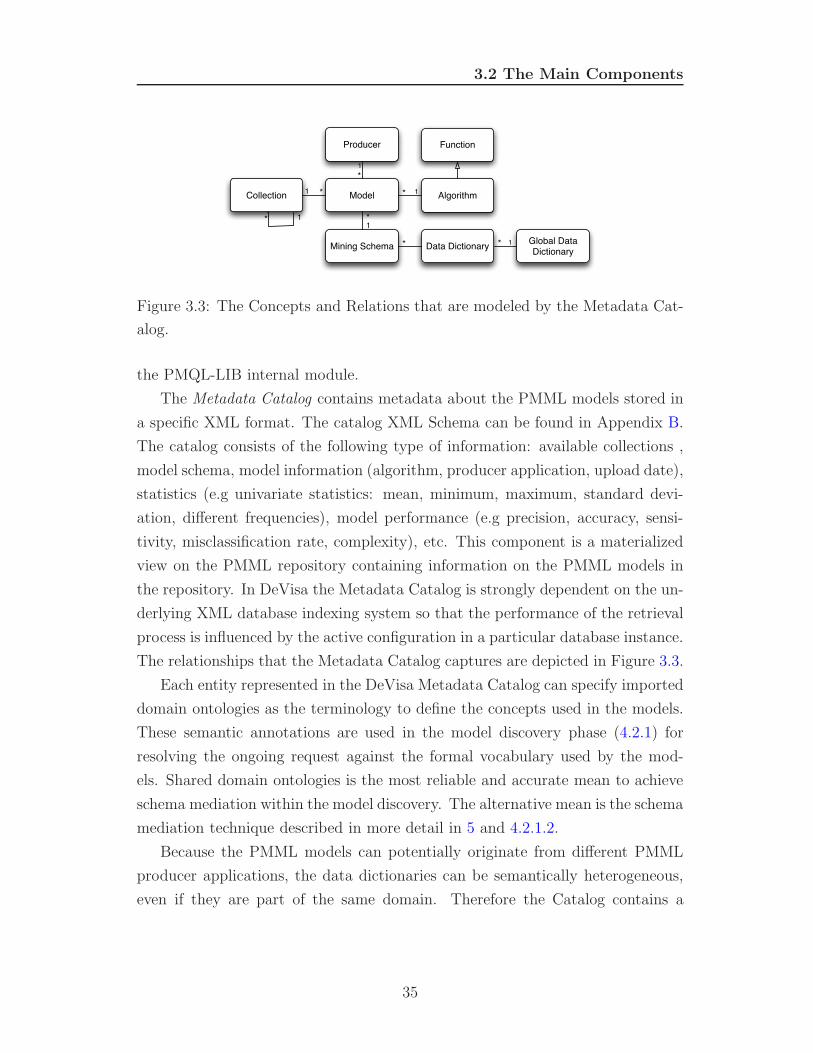
3.2 The Main Components
*
* 1
* 1
*1
*1
Producer Function
Model
Mining Schema
Algorithm
Data Dictionary
Collection
1
*1
Global Data Dictionary
*
Figure 3.3: The Concepts and Relations that are modeled by the Metadata Cat-
alog.
the PMQL-LIB internal module.
The Metadata Catalog contains metadata about the PMML models stored in
a specific XML format. The catalog XML Schema can be found in Appendix B.
The catalog consists of the following type of information: available collections ,
model schema, model information (algorithm, producer application, upload date),
statistics (e.g univariate statistics: mean, minimum, maximum, standard devi-
ation, different frequencies), model performance (e.g precision, accuracy, sensi-
tivity, misclassification rate, complexity), etc. This component is a materialized
view on the PMML repository containing information on the PMML models in
the repository. In DeVisa the Metadata Catalog is strongly dependent on the un-
derlying XML database indexing system so that the performance of the retrieval
process is influenced by the active configuration in a particular database instance.
The relationships that the Metadata Catalog captures are depicted in Figure 3.3.
Each entity represented in the DeVisa Metadata Catalog can specify imported
domain ontologies as the terminology to define the concepts used in the models.
These semantic annotations are used in the model discovery phase (4.2.1) for
resolving the ongoing request against the formal vocabulary used by the mod-
els. Shared domain ontologies is the most reliable and accurate mean to achieve
schema mediation within the model discovery. The alternative mean is the schema
mediation technique described in more detail in 5 and 4.2.1.2.
Because the PMML models can potentially originate from different PMML
producer applications, the data dictionaries can be semantically heterogeneous,
even if they are part of the same domain. Therefore the Catalog contains a
35

3.2 The Main Components
component called Global Data Dictionary (GDD), whose role is to provide unified
view on the data dictionaries.
The GDD acts like a mediator for the existing data dictionaries in DeVisa.
The mediator architecture conforms to a simplified GAV model, which is briefly
reviewed in 5.2. The implementation of the Global as View (GAV) mediator
architecture is depicted in Figure 3.4.
GDD
DD1 DD2 DD3
MS11 MS12 MS21 MS33MS32MS31
DeVisa Catalog
DeVisa Repository
...
Figure 3.4: The Global Data Dictionary as a mediator over the data dictionaries
in DeVisa.
The mediation occurs only at the semantic level, because both the global data
dictionary and the local ones are represented in the same XML schema. Therefore
the wrapper components are lightweight, their function resuming to seamlessly
mapping an entity in the global dictionary to the corresponding local one during
the PMQL query processing.
The GDD provides a matching between the fields in the data dictionaries,
including the derived fields in the transformation dictionaries. For each attribute
the matching is annotated with the confidence measure, meaning the degree of
similarity between the respective fields. An example of such a matching is de-
picted in Figure 3.5.
It is incrementally updated at the model’s upload time, when the newly up-
loaded data dictionary is merged into the existing GDD. If in the matching process
36

3.2 The Main Components
A B C E F
1 11
110.70.7
1
E F GDA B C
DD1 (MS11, MS12) DD2 (MS21)
GDD
Figure 3.5: An example of matching between the Global Data Dictionary and
the individual data dictionaries. Within a data dictionary mining schemas can
overlap. For instance, in DD1, field C is part of two mining schemas. The field
matches are annotated with the confidence factor. A field can match only one
entry in the GDD with confidence factor 1.
two or more attributes are found similar (match confidence is 1) then the GDD
retains only one entry for all the similar attributes. If the match confidence is
less than 1, GDD keeps all the attributes and annotates the matching with the
confidence factor. From this we can deduce that for any attribute in any data
dictionary there is exactly one GDD entry for which the match confidence is 1
and there can be more GDD entries for which the confidence factor is less than
1. The similarity of the fields is calculated using the technique described in 5.6
and memoization is used to store the results.
We observe from the algorithm 3.2.1 that two fields are considered to be
identical if the similarity between them is exactly 1, which can occur in three
different situations: when a field A ∈ D is copied in the Dg; when the two fields
refer the same term in a shared ontology; when the calculated similarity is higher
that cmax, which is a tuning parameter that in general has a value close to 1. The
last situation is necessary for very high similarity degrees that reflect irrelevant
37

3.2 The Main Components
Algorithm 3.2.1 The incremental update of the GDD when a new data dictio-
nary is uploaded in DeVisa
Input: D the data dictionary that is uploaded in DeVisa
Dg the existing global data dictionary as a view on the data dictionaries in
DeVisa
Output: An updated Dg view to integrate D
for all A ∈ D do
added← false
for all Ag ∈ Dg do
if ontologyTerm(A) = ontologyTerm(Ag) then
added = true
sim[A, AG] = 1
else
sim[A, Ag] = computeSimilarity(A, Ag)
if sim[A, Ag] ≥ cmax then
added = true
sim[A, AG] = 1
else
if sim[A, Ag] ≤ c then
sim[A, Ag]← 0
if added = false then
Dg ← Dg ∪ {A′}sim[A, A′] = 1
38

3.3 PMQL - A PMML Query Language
differences between the respective fields. For instance, if cmax = 0.99 and we
consider the fields microRNA and miRNA, representing the same entity and
having a similarity degree of 0.9939, then DeVisa memorizes the value 1. More
details on the computation of the similarity are given in 5.6.
The incremental update of the GDD maintains an up to date view that can
be queried during the online scoring, therefore decreasing the complexity of the
matching algorithm. The GDD is used only when in the match schema case,
when neither the schema nor the data dictionary are known. The GDD layer
provides an uniform pool of matching candidates, along with the pointers to the
actual fields.
The matching algorithm used in the incremental update of the GDD is fairly
close to the one used in the model discovery phase of the scoring. In the first case
the match is done between the existing GDD and the newly added data dictionary
and in the second case the matching is done between the consumer’s schema and
the GDD. On the contrary, the matching is used to produce a rather different
outcome. In the first case the outcome is the modified GDD to reflect the new
data dictionary, while in the second case the outcome is the transformation of
the consumer’s schema into the schema corresponding to the best matching.
3.3 PMQL - A PMML Query Language
For the purpose of interacting with PMML documents DeVisa defines a language
called PMQL (Predictive Model Query Language). PMQL is a query language
with an XML-based syntax. A PMQL query is executed against the DeVisa
repository of prediction models stored in PMML format. The result of a PMQL
query is also expressed in PMQL syntax.The PMQL schema and specifications
can be found in DeVisa. A consumer application wraps a PMQL query in a
SOAP message that invokes a service method and receives the answer as a PMQL
fragment wrapped in the SOAP answer.
DeVisa defines a XML-based language called PMQL (Predictive Model Query
Language) PMQL that is used to realize both the communication with the con-
sumer application and the internal communication between DeVisa components.
The consumer application expresses its goal in PMQL and wraps it in a SOAP
39

3.3 PMQL - A PMML Query Language
(*** (2007b)) message that is sent to the PMQL Web Service. The PMQL Web
Service forwards the PMQL goal to a DeVisa component called PMQL engine,
which is responsible with processing PMQL. It transforms the goal so that it
matches the existing DeVisa resources and, after successful matching, computes
the answer - also expressed in PMQL - that is transfered back to the consumer.
During processing the consumer’s goal is called query. The process is depicted in
Figure 3.6.
Depending on the task, a PMQL query specifies the target models it is based
on, such as the schema, the instances to predict etc. Bellow a simple PMQL
query fragment containing a classification task is presented. The full example is
listed in the PMQL use cases (DeVisa).
<pmql><request>
<score function="classification">
<modelSpec> <schema>
<field id="01" name="MFE"
opttype="continuous"
datatype="xs:float" usage="active">
<description>
Minimal free energy
</description> </field>
<field id="02" name="BN"
opttype="continuous"
datatype="xs:int" usage="active">
<description>
Number of Bulges
</description> </field> ...
</schema></modelSpec></score>
<data> <instance>
<field idref="#01" value="-20"/>
<field idref="#02" value="5"/>...
</instance> ...</data>
</request></pmql>
To resolve a scoring or composition goal, the PMQL engine performs the a
sequence of steps shortly described bellow. The first step is annotation, which
40

3.3 PMQL - A PMML Query Language
refers to checking the PMQL syntax and the integrity of the references to en-
tities in DeVisa. The rewriting identifies the desired task (scoring, composing
etc) and retrieves all the models that satisfy the query requirements. Within the
plan building phase an execution plan that involves specific models and XQuery
(XQuery) functions (for scoring or retrieving the models) is constructed. If an
implicit or explicit composition is necessary then an additional composing phase,
which assembles the base models, is performed. The execution invokes the nec-
essary XQuery functions against the repository of PMML models.
PMML model repository
Model Model
PMQL Web Service
Consumer
Goal
Concrete service
PMQL Goal
Query plan
PMQL Answer
PMQL Engine
Rewriter
ComposerExecuter
Plan Builder
...
Figure 3.6: Resolving consumers’ goals in DeVisa.
3.3.1 The Structure of a PMQL Goal
PMQL can express queries that correspond to core DeVisa functionality (See
3.1.1). In the case of a scoring goal, the PMQL query specifies the target models
41
3.3 PMQL - A PMML Query Language
it is to be executed on and the instances to predict. The target models are
described in a query via a model specification element. A model specification is
a set of restrictions used to identify a subset of models stored in DeVisa.
There are three ways in which a DM consumer application specifies one or
more models in DeVisa.
1. Exact Model. The query refers a model in the DeVisa catalog by its unique
name (through a XML reference). The DeVisa engine will use the specified
model to execute the scoring task.
2. Exact Schema. The query refers a mining schema (and therefore a data dic-
tionary) but does not refer a model. Nevertheless it can specify additional
desired properties through the use of filters. DeVisa engine will select the
appropriate model/models that conform to that particular schema. In its
current version PMML uniquely associates a schema to a model, but we
can foresee cases in which this association is not strict, i.e there are more
models that apply to the same schema and therefore the applications can
take advantage of this.
3. Match Schema. The query describes the required mining schema (the in-
stances to be scored conform to the mining schema). It can also specify
filters as in the previous case. In this case the DeVisa engine is responsible
for identifying the matching schema and the appropriate models (should
these exist). Moreover, the query can refer imported ontologies to explain
the requested mining schema, which needs to relate with the ones in DeVisa
Catalog. In this case the model is considered to be laxly specified. There
are two possible degrees of specificity: the data dictionary is common to the
goal and DeVisa or it needs to be matched. Hence we identify two possible
sub-cases:
• Exact Data Dictionary. In this case the goal specifies a data dictionary
in DeVisa and specify a schema within that specific data dictionary.
This approach simplifies the model discovery phase because the search
is limited within a known vocabulary. The engine will try to match
all the DeVisa schemas with the one specified by the consumer. If
42

3.3 PMQL - A PMML Query Language
composition is allowed, even if there is no schema that matches exactly
the one specified by the consumer, there is a chance that a model
conforming to the consumer’s schema can be built on the fly (see 4.3).
• Match Data Dictionary. This case adds another layer of complexity
atop the previous case, in the sense that the engine first needs to find
a data dictionary in DeVisa that matches the one specified by the
consumer. The names do not necessarily need to coincide, unless this
is explicitly requested in the consumer’s goal. For each of the matching
data dictionaries, the previous step is applied in order to identify the
corresponding models.
As stated above, in the case of a scoring task, the PMQL query needs also
to specify the instances to score. The set of instances need to conform to the
specified mining schema.
3.3.2 PMQL Query Processing
The DM Consumer sends a SOAP message that wraps the request for a scor-
ing task expressed in PMQL. The PMQL scoring query is transmitted to the
component responsible with processing and resolving PMQL requests, which is
called PMQL engine. The internal mechanism of the PMQL engine is presented
in Figure 3.7.
The phases in which the PMQL engine executes a scoring query are:
3.3.2.1 Annotation
This phase includes the PMQL syntactic validity check as well as the integrity
of XML references. XML references occur in a PMQL query when the consumer
specifies exactly the models to score on, or the mining schema of the model to
score on. This phase involves querying the Metatada Catalog (Figure 3.7).
The semantic checking involves a look-up in the repository catalog for a model
that satisfies the query constraints (function type, accuracy, complexity, fresh-
ness) and whose schema matches the query schema. The look-up can be strict
43

3.3 PMQL - A PMML Query Language
getScoringFunction
executeScoringFunction
getApplicableModels
PMQL Engine
Annotator
Rewriter
Plan Builder
Plan Executer
Metadata Catalog
XQuery Library
PMML Repository
PMQL
PMQL
PMQL
Figure 3.7: The internal mechanism of the PMQL engine.
(exact matching of the schemas) or lax (compatible schemas). If the lax look-
up is enabled then the schemas need only to be compatible with respect to the
number of fields and field types. Should this be the case the subsequent phase
performs the actual mapping between the fields of the two schemas.
If several models fulfill the query requirements, a sequence of model references
is returned. If no model entry is complying with the requested properties found
in the catalog, a null reference is returned and the execution of the current query
stops.
3.3.2.2 Rewriting
The rewriting phase treats the case in which the models are laxly specified. In the
exact schema case the model references applied to the schema are retrieved and
replaced in the PMQL query. In the match schema case, the engine looks in the
Metadata Catalog for a DeVisa mining schema that matches the specified one. As
a general rule, rewriting refers to reinterpreting the PMQL requirements in terms
of the DeVisa Metadata Catalog and replacing the model requirements in the
44

3.3 PMQL - A PMML Query Language
query with concrete model references in the PMML model repository. Annotation
and rewriting are also called model discovery and the schema rewriting technique
is described formally in 4.2.1.
This phase involves solving the schema differences between the query and
the sequence of models returned in the first phase, provided that the look-up
procedure is lax and and there is one or more predictive models satisfying the
request. Basically the goal is to rewrite the query in terms of the matching
models. The possible dissimilarities can refer to the names, the types or the
mining properties of the fields. A subset of type differences can be resolved by
applying the allowed type conversions as specified in the XMLSchema.
DeVisa uses the following strategy in resolving the field dissimilarities.
In the first phase the engine establishes all the candidate matches between
the fields in the consumer’s schema and the fields in the GDD. The matches are
annotated with the degree of confidence. The notion of a match refers strictly
to similarity, therefore the confidence factor measures how similar two fields are.
The similarity is calculated based on name, textual description of the fields, field
statistics, and the values in the consumer’s data (see 5.6).
In the second phase the matches are translated to the actual data dictionaries
based on the existing GDD view, so it obtains the actual matches between the
fields in the consumer’s schema and the ones in the dictionaries along with the
confidence factors. For each field there are several potential matches, each of
them annotated with a confidence factor.
In the third phase, it attempts to build a schema mapping by trying to find
the best mapping (with the best confidence factor, calculated as the sum of the
confidence factors of the individual field mappings) to a data dictionary and a
mining schema. So the resulting matching needs to map consumer’s schema into
one and only data dictionary. This cannot always be achieved, since it is possible
that the individual field mappings span through several data dictionaries and a
model that can be applied to the schema does not exist. If several such mappings
exist, the one with the highest confidence factor is selected.
The detailed algorithm is presented in 4.2.1.2.
On the other side, the consumer’s goal can specify if the composition of models
is allowed. In this is the case, if a mapping within the same data dictionary can
45

3.3 PMQL - A PMML Query Language
be found, then the composer component can attempt to build a new model based
on existing ones in case no model exists on the respective schema.
The outcome of this phase is a rewritten PMQL query (or a sequence of
queries) which is (are) reinterpreted and transformed with respect to the internal
schema of the matching PMML model (or models) in the DeVisa repository.
3.3.2.3 Plan Building
This phase builds the PMQL query plan from a rewritten PMQL document. It
reorganizes the document so that each model reference is associated with the
appropriate instances to score. If the DeVisa schema specifies a transformation
dictionary for certain attributes in a model, then the values of the attributes in the
instances are mapped into another domain according to it. The transformations
applied to the instances must be equivalent to the transformations applied when
the model was created. DeVisa implements the transformations through the
use of XQuery extension mechanisms available in eXist. The query plan is an
XML document that can be directly passed to the DeVisa XQuery library in the
execution phase.
3.3.2.4 Plan Execution
For each of the models in the PMML model repository that were identified in the
rewriting phase it executes the appropriate XQuery scoring function stored in
the DeVisa library. The scoring result is added to the PMQL document (that is,
the scoring result is paired with the instance). Expressing the scoring algorithms
on the PMML models in XQuery leverages the underlying XML database query
optimization.
46

3.4 Predictive Models Composition
3.4 Predictive Models Composition
3.4.1 Methods and Challenges In Composing Data Min-
ing models
In general the composition of prediction models can be realized in various ways.
They all have in common the goal of making predictions more reliable. Com-
posing several prediction models means merging the various outputs into a single
prediction.
Several machine learning techniques do this by learning an ensemble of models
and using them in combination. The most popular are bagging, boosting and
stacking (a brief overview over the major methods can be found in Ian H. Witten
(2005)).
Bagging (Breiman (1996)) applies an unweighted voting scheme on the out-
comes of different classifiers built on possibly different data sets (which can be
obtained by resampling the original data set). In the case of numeric prediction,
instead of voting on the outcome, the individual predictions, being real numbers,
are averaged. The component models are usually built separately.
Boosting (Freund & E.Schapire (1997)) also uses voting or averaging schemes
to combine the outcomes, but, unlike bagging, it uses weighting to give more
influence to the more successful models. Furthermore the process is iterative,
each component model is built upon the previous model and therefore influenced
by their performance.
Stacking (Wolpert (1992)) applies on heterogeneous classifiers and trains a
new meta learner on the predictions of the component classifiers using a valida-
tion data set. The meta learner can be of various types depending on the set
of attributes used for meta learning. Some meta-learners use only the class pre-
dictions of the component models for training, while others use both the class
predictions and all the original input attributes. It applies both to categorical
and numeric predictions.
Another approach which is mostly useful in distributed data mining is com-
bining models with various levels of granularity. For instance, it might be the
case that a model classifies an instance at a coarse level, while another model
47

3.4 Predictive Models Composition
does it with a finer granularity. One can use the first model to tag the instances
with a more general class and then to use a specialized classifier for each of the
resulted groups. This technique is also useful in classification when an algorithm
cannot predict multi-class attributes, such as standard SVM. Another direct use
of this technique is model selection in PMML, which is described in 3.4.2.
In the distributed data mining model there are situations when different mod-
els are built on vertically fragmented data (usually that reside at different sites).
Each of the individual models is built on projections on the same relation, but
unable to detect cross-site correlations. A meta-learning approach has been pro-
posed in Prodromidis et al. (2000) that uses classifiers trained at different sites
to develop a global classifier. DeVisa addresses vertically partitioned data only
in certain configurations, as described in 3.4.3.
Another possibility to combine data mining models is to adjust a given model
to a consumer’s specific needs. This is called model customization. This is the
situation in which a model consumer repeatedly uses the model in its knowledge
integration processes and may collect information on its performance. A new
model can be constructed based on the specific needs for the consumer. The
producer’s data can be combined with the consumer’s data to build a new cus-
tomized model. The same principle applies to refreshing a model to reflect the
new trends in the data; thus either a new model is built of the new data, or the
new data is merged with the old one to adjust the model. This is related to the
concept of incremental data mining, which was introduced in M.Harries et al.
(1998). A related approach can be found in Kuncheva (2004), where strategies
for building ensembles of classifiers in non-stationary environments in which even
the classification task may change are presented.
DeVisa only stores the prediction models, not the original training data they
were built on. Therefore we consider the training data as not being available.
Subsequently the model composition in DeVisa is limited to certain techniques
which are described in 3.4.3. However the consumer application can build new
models based on the existing DeVisa models and its own validation set.
48

3.4 Predictive Models Composition
3.4.2 Model Composition in PMML
3.4.2.1 Model sequencing
Model sequencing is the process through which two or more models are combined
into a sequence where the results of one model are used as input in another model.
Model sequencing is supported partially by the PMML specification (PMML).
Examples of sequencing include:
• The missing values in a regression model can be replaced by a set of rules
(or decision tree)
• Several classification models with the same target value can be merged via
a voting scheme, i.e the final classification result can be computed as a an
average of the results of the initial classifiers.The average can be computed
by a regression model.
• Prediction results may have to be combined with a cost or profit matrix
before a decision can be derived. A mailing campaign model may use tree
classification to determine response probabilities per customer and channel.
The cost matrix can be appended as a regression model that applies cost
weighting factors to different channels, e.g., high cost for phone and low cost
for email. The final decision is then based on the outcome of the regression
model.
3.4.2.2 Model selection
Model selection is the process of combining multiple ’embedded models’, such as
model expressions, into the decision logic that selects one of the models depending
on the current input values. For instance, a common method for optimizing
prediction models is the combination of segmentation and regression. Data are
grouped into segments and for each segment there may be different regression
equations. If the segmentation can be expressed by decision rules then this kind
of segment based regression can be implemented by a decision tree where any leaf
node in the tree can contain an embedded regression model.
49

3.4 Predictive Models Composition
PMML version 3.2 supports the combination of decision trees and simple
regression models. More general variants would be possible and may be defined
in future versions of PMML.
In PMML model composition uses three syntactical concepts:
• The essential elements of a predictive model are captured in elements that
can be included in other models,
• Embedded models can define new fields, similar to derived fields and
• The leaf nodes in a decision tree can contain another predictive model.
3.4.3 Model Composition in DeVisa
DeVisa supports the two types of composition methods described in the PMML
specifications: model sequencing and model selection. As seen in 3.4.2 the current
version of PMML supports the combination of decision trees or rules and simple
regression models.
Model sequencing is the case in which two or more models are combined into
a sequence where the results of one model are used as input in another model.
In DeVisa it is very often an intrinsic part of a model, namely a transformation
function, as formalized in 4.3. For instance, a supervised discretization algorithm
is applied to a certain attribute and this algorithm is described within a trans-
formation dictionary. Another common way to use sequencing is to fill missing
values for an attribute if the model can be applied only on attributes without
missing values. A transformation function made of decision rules is applied on
the values of the respective attribute.
Model selection is when one of many models can be selected based on decision
rules.
A common model selection method for optimizing prediction models is the
combination of segmentation and regression. The data set is separated into seg-
ments and for each segment a regression equation is applied (segment based re-
gression). It can be implemented in PMML by a decision tree (describing the
segmentation rules) where any leaf node in the tree can contain an embedded
50

3.4 Predictive Models Composition
regression model. This scenario can be seen as an instance of composition of
models with various levels of granularity.
The producer applications can upload composite models in DeVisa, as long
as the models are expressed in well formated PMML. In this section we focus
moreover on the situations in which DeVisa is responsible for composing the
models.
Depending on the moment when the composition process occurs, we can fur-
ther classify the composition in DeVisa in implicit or explicit composition (Gorea
(2008d)). All types of model composition occur within the same DeVisa data dic-
tionary. There are multiple challenges and limitations in performing a accurate
and flexible model composition. The most important of these is schema difference
between the consumer’s goal and the DeVisa catalog. The difference manifests
itself either at the level of vocabularies or at the data granularity level.
3.4.3.1 Implicit Composition
Implicit composition is the situation when the models are composed within the
orchestration of the scoring or search service (see 3.1.1).
3.4.3.2 Explicit Composition
Explicit Composition is when a DM consumer explicitly specifies in its goal that a
composition is desired. The composition query usually includes the models to be
composed, the composition method and a validation data set. DeVisa identifies
the specified models and checks them for compatibility. If all the prerequisites for
the composition are fulfilled then a new valid model is returned to the user/stored
in the repository.
An explicit composition scenario occurs when a consumer wants to make the
best out of several heterogeneous models in DeVisa complying to the same mining
schema.
51

Chapter 4
DeVisa - Formal Model
4.1 Overview of DeVisa Concepts
A DeVisa data dictionary is a tuple D = (U, S, T, F) where:
1. U is a finite set of attributes U = {A1, A2, . . . , An}, ∀Ai, i = 1, . . . , n, ∃dom(Ai),
called the domain of Ai. Within a data dictionary, the names of the at-
tributes must be unique.
2. S is a finite multi-set of mining schemas S = {S1, S2, . . . , Sm}, where Si =
(Ui, Pi), Ui ⊆ U, and Pi is a set of properties related to the attributes in Ui,
i = 1, . . . , m.
Given a mining schema S = (U, P ) and A ∈ U , P (A) signifies the subset of
P with the properties applicable to the attribute A.
The properties of an attribute refer to additional constraints besides the
ones in the data dictionary that usually refer to the behavior of the data
mining algorithm when handling the values of that particular attribute (e.g
independent attribute, predicted attribute, or excluded). Examples of at-
tribute properties are usage(A) = predicted,missingV alueTreatment(A) =
asIs or outliers(A) = asExtremeV alues.
We consider a multi-set of mining schemas to ensure compatibility with the
PMML specification.
52

4.1 Overview of DeVisa Concepts
3. T is a sequence of transformation functions applicable on the attributes.
T = (T1, T2, . . . , Tm). The transformation functions are used in order to
map user data to values that are easier to use in specific models. DeVisa
allows various types of data transformations that are supported by the
PMML specification: normalization, discretization, value mapping, func-
tion, aggregation. There are three types of transformations:
(a) Single attribute transformations. For each Ai, i = 1, n we consider
Ti : dom(Ai)→ dom(Bi). Bi is called a derived attribute and is further
referred in the mining models. For convenience we assume the identity
function for the attributes that do not define transformations. Exam-
ples of such transformations are: normalization, discretization, value
mapping.
(b) Multiple attribute transformations. Ti : dom(Aii)× · · · × dom(Aik)→dom(B). B is also called derived attribute. This type of transforma-
tion includes functions and for each tuple in the relation the value of
the function is calculated and a new relation is built considering the
transformation.
(c) Multiple tuple transformations. This type of transformations are called
aggregations and are similar to the group functions in SQL, such as:
count, sum, average, min, max or multiset.
The transformations are applied to the data set prior to the model itself
in the order they were presented, i.e the single attribute transformations,
followed by the multiple attribute transformations and the multiple tuple
transformations.
4. F is a set of constraints. F corresponds to the structural relationships,
constraints and rules expressed via ontologies or taxonomies.
The PMML specification includes a taxonomy element that can describe
parent-child relationships between the values of categorical fields used in a
data dictionary. In DeVisa the data dictionaries can refer domain ontologies
through the use of PMML extension mechanism.
53

4.1 Overview of DeVisa Concepts
Definition 4.1 The Global Data Dictionary (GDD) is the uple Dg = (Ug, M),
where Ug is the set of entries (attributes) in the GDD, M : Ug → 2U1∪U2∪···∪Uk ,
A ∈ M(Ag) if sim(Ag, A) ≥ c, where sim is the similarity function defined in
5.6, and U1, U2 . . . Uk are the set of attributes in the DeVisa data dictionaries.
Intuitively, the GDD associates each field in each data dictionary or derived
field in any transformation dictionary with one or more entries in the GDD. Each
association is annotated with a similarity confidence factor in [0, 1]. It is not
possible that a field is associated with two or more GDD entries with similarity
confidence factor 1. An example of such a matching is presented in Figure 3.5.
As it can be observed in the figure, the GDD can be modeled as a edge-weighted
bipartite graph. The set of attributes includes the derived attributes in the data
dictionaries as well, which are not explicitly mentioned for brevity.
A DeVisa Metadata Catalog is an uple DS = ({D1, D2, . . . , Dk}, Dg) where
D1, D2, . . . , Dk are DeVisa data dictionaries and Dg is the global data dictionary.
Given a mining schema S = (U, P ), with U = {A1 . . . An} we define a model
on S as a function ϕ : dom(Ai1)× dom(Ai2)× · · · × dom(Air)→ C, where C is a
set defined as:
1. if ϕ is a classification or regression model, then ∃A ∈ U so that C = dom(A)
- in this case A is the class (predicted) attribute and r = n− 1;
2. if ϕ is a clustering model, then C is a finite set of cluster tags and r = n.
According to the PMML specifications, each model needs to specify its own
mining schema. Although from a theoretical perspective it is possible that several
models apply to the same mining schema, we will assume that there is a one to one
correspondence between the models and the mining schemas in DeVisa. Therefore
the multi-set approach in the above definition.
Given a data dictionary D = (U, S, F) we consider a set Ψ = {ϕ1, ϕ2, . . . , ϕm}of models applicable to the mining schemas in S.
⋃
Di∈DS Ψi is called the DeVisa
PMML Repository.
A tuple on U is a set {A1 : x1, A2 : x2, . . . , An : xn} so that xi ∈ dom(Ai).
A relation on the data dictionary D = (U, S, F) is a set R of tuples on U that
satisfy the restrictions in F.
54

4.1 Overview of DeVisa Concepts
A relation (or dataset) on a mining schema S = (U, P ) is a set of tuples R
that satisfy the restrictions in F[U ].
4.1.1 The connection between the mining models and func-
tional dependencies
This section introduces the concept of mining functional dependencies and draws
a framework in which new mining functional dependencies can be inferred from
a data dictionary. We will focus only on classification and regression models.
Given a mining schema S = (U, P ), U = {A1 . . . An} in a particular data
dictionary and a classification/regression mining model ϕ defined on S, we can
draw a connection with the functional dependency, i.e A1 . . . An−1 → An, where
A1 . . . An are the active attributes and An is the predicted attribute (class at-
tribute). The information on whether an attribute is active or predicted is found
in the set of properties P associated with each mining schema.
Let us recall the definition of a functional dependency in the relational model.
If X, Y are sets of attributes, we say that a relation R satisfies the functional
dependency X → Y if for any tuple t1, t2 ∈ R so that t1[X] = t2[X], it results
that t1[Y ] = t2[Y ]. The representation of mining schemas using functional depen-
dencies is rather natural, considering that, for a given tuple, the class attribute
values are calculated from the active attribute values based on the given model.
Subsequently, if two tuples have equal values on the active attributes, the model
will deterministically produce the same values for the class attributes - actually
the functional dependency is self-fulfilling. We are dealing with a simplified form
of functional dependencies, in which the right side is formed by a single attribute
(actually any functional dependency can be reduced to this form using the de-
composition rule of inference). We will name this type of functional dependency
as mining functional dependency (MFD).
Definition 4.2 Given a mining schema S = ({A1 . . . An}, P ) so that usage(An) =
predicted, a model ϕ : dom(A1)× dom(A2)× · · · × dom(An−1) → dom(An). We
will denote a mining functional dependency as A1 . . . An−1 →m An.
55

4.1 Overview of DeVisa Concepts
If R is a relation defined on U , then R satisfies the mining functional depen-
dency A1 . . . An−1 →m An if
∀t ∈ R we have ϕ(t[A1 . . . An−1]) = t[An]
Proposition 4.1 If R satisfies the MFD A1 . . . An−1 →m An, then R satisfies
the FD A1 . . . An−1 → An.
Proof. Let’s consider t1, t2 ∈ R so that t1[A1 . . . An−1] = t2[A1 . . . An−1].
R satisfies the MFD A1 . . . An−1 →m An, so ϕ(t1[A1 . . . An−1]) = t1[An] and
ϕ(t2[A1 . . . An−1]) = t2[An]. From ϕ(t1[A1 . . . An−1]) = ϕ(t2[A1 . . . An−1]), it re-
sults that t1[An] = t2[An]. So R satisfies the FD A1 . . . An−1 → An. �
Let us note that the reverse is not necessarily true. From Proposition 4.1
it results that we can apply the functional dependency properties in the case of
MFDs and use some of the formalisms present in the FD theory in DeVisa.
The set of properties that can be translated to our representation with mining
functional dependency is:
1. Reflexivity. ∀R relation, satisfies A1 . . . An → Ai, ∀i = 1, . . . n
2. Extension. If R satisfies X → A then If R satisfies XY → A.
3. Extended Transitivity. If R satisfies X → A and AY → B, then R satisfies
XY → B. If Y = Φ, then we have the classical transitivity.
4. Reverse Projection. If R[Z] satisfies X → A, then R satisfies X → A.
We included only the properties that are relevant to our representation.
Using this representation, we can express a data dictionary D as a set of
mining functional dependencies, where each of them is the translation of a mining
schema. In practical cases the set of MFDs does not result in integrity constraints
on given relations, as in the relational model case. As we mentioned before, the
MFDs are self-fulfilling, i.e for a given relation (which is normally part of the
consumer’s goal) the model itself will produce precise values for the attribute at
the right side of the MFD. So most of the relations that the system interacts
with will satisfy an individual MFD. Although we can consider a data dictionary
56

4.1 Overview of DeVisa Concepts
as a set of MFDs that hold simultaneously in given relations, the approach does
not have too much practical relevance. Therefore a statement like a relation R
satisfies all the MFDs in the data dictionary D, which is very common in the
relational theory, will not hold in our approach.
Moreover, DeVisa is a dynamic environment, in which new models with new
mining schemas (and therefore new MFDs) can be added any time. The upload
of new models would invalidate a potential (previously established) property of
satisfiability of a set of MFDs on a given relation.
In somewhat the same category is the notion of consequence, which is central
in the relational theory. A functional dependency Sr expressed as A1 . . . An → B
is a consequence of D if every relation that satisfies the dependencies in D satisfies
also Sr. The concept of consequence has the notation D |= Sr. In DeVisa the
concept of consequence also holds, although in practice it is rarely the case that
a relation R needs to satisfy simultaneously all the MFDs in D (so the premise
does not hold). Therefore we are moreover interested in weaker premises, such
as conveniently chosen subsets of D.
In the composition of mining models (see 3.4.3, 4.3) we are interested in
deducing a new mining schema that correspond to a given consumer’s goal from
a DeVisa data dictionary (or set of MFDs). This problem can be solved using
the inference rules in the functional dependency theory.
Armstrong’s axioms (Armstrong (1974)) form a sound and complete set of
inference rules that can be also applied to MFDs.
A1 Reflexivity. If Y ⊆ X then X →m Y
A2 Decomposition and union.
If X →m Y Z then X →m Y and X →m Z.
Reversely, if X →m Y and X →m Z then X →m Y Z.
A3 Transitivity. If X →m Y and Y →m Z then X →m Z.
If A is the Armstrong set of inference rules and D a set of MFDs, we say
that the MFD X → A can be derived from D using rules from A if X → A is
57

4.2 The Scoring Process
obtainable by means of repeatedly applying the inference rules in A to functional
dependencies in D. We denote the derivation by D ⊢A X → A.
If X is a set of attributes, then we denote X+A = {A|D ⊢A X → A}.
This approach becomes very useful in the query rewriting phase of the scoring
process, when a consumer mining schema needs to be matched with a mining
schema in the data dictionaries (see 4.2.1). Each potential matching needs to be
validated using the functional mining schema approach, which can be reduced to
verifying if a certain attribute A can be determined from a set of attributes X
using the MFDs in D.
4.2 The Scoring Process
From a theoretical perspective, the scoring procedure consists of:
1. identification of a subset of models in DeVisa that satisfy the model speci-
fications in the query (filters and matching schemas);
2. scoring each of the models on the dataset specified in the query.
Definition 4.3 A scoring query is a tuple (MSpec, R), where
• MSpec is the model specification, defined as
MSpec ::= MRef | (Filter, SRef | (DRef, S | S))
where MRef is a reference to a model (corresponding to the Exact Model
case), Filters is a set of filters corresponding to the additional properties
that the model needs to conform to, SRef is an reference to a mining schema
(Exact Schema case), and S describes a mining schema (Match Schema
case) that needs to be matched against one in the DeVisa Catalog. The
cases are described in 3.3.1
• R is the dataset to score.
58

4.2 The Scoring Process
4.2.1 Model Discovery
The model discovery problem is that, given a scoring query, the engine needs to
find the models that satisfy the query requirements and adjust the query in terms
of the found models if it is the case.
Let’s assume for simplicity reasons that the scoring query does not allow model
composition (the compose attribute is set to false). The model composition case
is described in the subsequent section (4.3). The main challenge is identifying
the appropriate models in the Match Schema lax model specification case (see
3.3.1). In this case it is not known if the schema given in the request conforms
to a certain DeVisa data dictionary. The engine should check for an appropriate
matching schema in all the data dictionaries. DeVisa allows that the fields in
the data dictionary (and therefore mining schemas) to refer terms in domain
ontologies via XML references. Therefore the match between schema elements
can be achieved easily in the case in which the consumer’s goal refers terms in
the same ontology.
We are going to describe the model discovery process taking into consideration
the consumer’s model specification presented at the beginning of the current
section.
4.2.1.1 Exact Model or Exact Schema Case
If the scoring query refers an exact model through MRef , then the model dis-
covery resumes to finding the respective model ϕ in the repository and scoring
the data set R on ϕ.
If the scoring query specifies an exact schema through SRef , then the the
engine finds all the models complying to the specific mining schema and applies
them on R. Since The PMML specification defines each mining schema within
a specific model, that would reduce this case to the previous one. Our formal
model also assumed a 1 : 1 correspondence between the mining schemas and
the mining models. On the other side the data dictionaries contain multi-sets of
mining schemas. Therefore DeVisa uses the mining schema equality to extend
the search to equal mining schemas within the same data dictionary. Two mining
59

4.2 The Scoring Process
schemas S1 = (U1, P1) and S2 = (U2, P2), belonging to the same data dictionary,
are equal if U1 = U2 and P1 = P2.
4.2.1.2 Match Schema Case
Here we further distinguish two sub-cases depending on whether a reference to a
DeVisa data dictionary is provided in the consumer’s query.
First, if the data dictionary is referred by the query through DRef , the lookup
is restricted within that specific data dictionary. Secondly, if the data dictionary
is not specified in the consumer’s query, the lookup is slightly more complicated,
in the sense that a matching mining schema in any of the DeVisa dictionaries
needs to be found. The first case is a simplified configuration of the second case.
Therefore in the following we will consider the general case when the data
dictionary is not specified. We will provide the general theoretical approach for
the model discovery problem and then we will particularize for the first case. So
the model discovery problem (without model composition) can be articulated as
follows.
Given a set of DeVisa data dictionaries D1, D2, . . .Dn, where Di = (Ui, Si, Fi)
where i = 1, n, the corresponding set of models Ψ1, Ψ2, . . .Ψn, a mining schema
Sr and Rr a relation on Sr, find {ϕ1, . . . ϕk} so that ϕi, i = 1 . . . k is best applicable
on Rr. Furthermore, assuming the existence, the engine needs to determine all
the models corresponding to the schemas equivalent with all Si, i = 1 . . . k in their
respective data dictionary.
In order to define the concept of best applicable, we need to provide a set of
other definitions.
Definition 4.4 Given two sets of attributes Ur and U (Ur is the set of attributes
to be transformed), c, s ∈ [0, 1], a match function with support s and confidence
c is a partial bijective function µ : Ur → U so that s ∗ |Ur| ≤ |µ(Ur)| defined as
if µ(Ar) = A then sim(Ar, A) ≥ c
The values c and s are tuning parameters, c represents how similar the fields
need to be and s is the fraction in which the consumer’s schema needs to be
60

4.2 The Scoring Process
covered by the matching. Intuitively, the more attributes are matched, the better
the matching is.
We consider a partial function as a function in which not every element of
the domain has to be associated with an element of the codomain. However, for
each of the field elements of the codomain, there is exactly one field element in
the domain that maps to it.
Definition 4.5 A match function µ : Ur → U is valid if ∃Di data dictionary
having the set of attributes Ui so that U ⊆ Ui.
Definition 4.6 Given a consumer’s mining schema Sr = (Ur, Pr), a DeVisa
mining schema S = (U, P ) and c, s ∈ [0, 1], we say that Sr matches S with
support s and confidence c if both of the following are true:
1. s|Ur| ≤ |U | ≤ |Ur| and
2. ∃µ : Ur → U ′, match function with support s and confidence c so that U ⊆U ′ and
3. ∀Ar ∈ Ur and A ∈ U so that µ(Ar) = A, we have Pr(µ(Ar)) ⊆ P (A)
In another words, a consumer schema matches a DeVisa schema if, for a subset
of the fields of size s∗Ur, a similarity measure can be calculated, its value is lower
than a given threshold and the requested mining constrains are lesser that the
ones in the DeVisa repository. In DeVisa the sim function between two fields has
values in the interval [0, 1] and is calculated using the technique described in 5.6.
Definition 4.7 Given a model ϕ defined on the mining schema S in the data
dictionary D = (U, S, T, F), a consumer’s schema Sr, a relation Rr defined on Sr
and s, c ∈ [0, 1], we say that ϕ is applicable on a dataset Rr if:
1. Sr matches S with support s and confidence c;
2. IS(Rr) satisfies the restrictions in F, where IS(Rr) is the interpretation of
Rr in terms of the mining schema S.
61

4.2 The Scoring Process
As we see from the previous definitions, s and c are fixed thresholds for de-
ciding if two schemas match or not. For two schemas there can be more match
functions with support s and confidence c. We are further interested to find the
degree of actual confidence with which two schemas match.
Definition 4.8 The actual confidence of a match function is calculated as the
average of the similarity degree between any pair of fields that map to each other:
conf(µ) =1
|Ur|∑
Ar∈U ′
r
sim(Ar, µ(Ar)), (4.1)
where U ′r = {Ar ∈ Ur s.t ∃A ∈ U s.t µ(Ar) = A}
To be observed that the actual confidence is proportional with the actual
support, since the numerator grows with the number of attributes matched.
Definition 4.9 Given two mining schemas Sr and S and µ1, . . . , µt the match
functions between Sr and S, we say that Sr matches S with the actual confidence
conf(Sr, S) if
conf(Sr, S) = maxi=1,tconf(µi)
The match functions with the actual confidence conf(Sr, S) are called optimal
match functions.
Definition 4.10 Given a model ϕ defined on the mining schema S, a consumer’s
schema Sr, a relation Rr defined on Sr and s, c ∈ [0, 1], we say that ϕ is best
applicable on a dataset Rr if:
1. ϕ is applicable on Rr
2. conf(Sr, S) = maxSr matches S′
conf(Sr, S′)
Otherwise stated, Sr matches S with the highest actual confidence.
Since we need to find one or more models which are best applicable on a
schema, we are always interested in the optimal match functions, i.e the ones
that map Sr into schemas in DeVisa with the highest actual confidence.
62
4.2 The Scoring Process
Definition 4.11 Given Sr a consumer’s schema, the set of optimal match func-
tions for Sr is
{µi|i = 1, . . . , l}, where µi : Ur → Ui so that conf(µi) = maxµ : Ur→Uconf(µ)
where U is a set of attributes in DeVisa.
The optimal match function is to some extent analogous to the Match operator
introduced in Rahm & Bernstein (2001) and recalled in 5.3. An overview of the
state of the art in schema/ontology mediation and the general context in which
this problem is modeled in DeVisa are presented in 5.3.1 and 5.4 respectively.
An algorithmic approach to calculate the optimal match function µ is de-
scribed in 5.5. However in this general process of calculating the match function,
a few functional considerations need to be taken into account. These are sum-
marized in the isDerrivable function called in the algorithm 5.5.3.
It is a decision function on whether a given mining schema obtained from the
consumer’s schema through the match function µ can be derived from the mining
schemas in a data dictionary. The result of the decision depends strongly on if
composition is allowed by the consumer’s request. In this section we focus on the
simple case when composition is not allowed.
We will use the mining functional dependency representation described in
4.1.1. We recall that in this representation a mining schema is abstracted to a
functional dependency, whereas data dictionaries are abstracted to sets of func-
tional dependencies.
Before giving the definition let’s denote by µ(Sr) = (µ(Ur), µ(Pr)) the mining
schema obtained from Sr after applying µ. µ(Ur) is the co-domain of the matching
function as shown in algorithm 5.5.3 and µ(Pr) is obtained through translating
the properties in Pr in terms of the attributes in the co-domain.
Definition 4.12 Given a consumer’s schema Sr = (Ur, Pr), a data dictionary
Di having the set of attributes Ui, a valid match function with support s and
confidence c µ : Ur → U ′i , where U ′
i ⊆ Ui. Let Let X →m A be the MFD associated
with the mining schema µ(Sr) and Di the set of MFDs associated with Di.
We say that µ(Sr) is derivable without composition from Di if
63

4.2 The Scoring Process
1. ∃Y →m A ∈ Di so that Y ⊆ X and
2. s ·|Ur| ≤ |Y |+ 1
In another words, µ(Ur) can be obtained by applying in one step the extension
inference rule from Y →m A, or using Armstrong’s axioms, in two steps, by
applying reflexivity and transitivity. The condition 2 refers to maintaining the
support factor s specified by the consumer, even if we cut off attributes from the
rewritten consumer’s schema µ(Ur). Checking if µ(Ur) is derivable from D his
can be achieved in O(n|Ur|), where n is the number of MFDs in D.
Proposition 4.2 Given Sr = (Ur, Pr) a consumer’s schema, Di a data dictio-
nary. It exists µ : Ur → Ui a valid match function with confidence c and support
s so that µ(Sr) is derivable without composition in Di if and only if ∃S ∈ Di so
that Sr matches S with confidence c and support s.
Proof. First let us assume that ∃µ so that µ(Sr) derivable without composi-
tion in Di and prove that ∃S ∈ Di so that Sr matches S.
Let X →m A be the MFD associated with µ(Sr). Then ∃Y →m A ∈Di so that Y ⊆ X and s · |Ur| ≤ |Y |+ 1.
Let S = (U, P ) be the mining schema corresponding to Y →m A. We prove
that Sr matches S with confidence c and support s.
U = Y ∪{A} ⊆ X∪{A} = µ(Ur). µ match function, so s|Ur| ≤ |µ(Ur)| ≤ |Ur|.Then it follows that |U | ≤ |Ur|.
But s · |Ur| ≤ |Y | + 1 = |U |. We proved the first condition in the definition
4.6.
The second condition in definition 4.6 results from µ : Ur → X ∪ {A} and
U = Y ∪ {A} ⊆ X ∪ {A}.Conversely, let us assume that ∃S = (U, P ) ∈ Di so that Sr matches S and
prove that ∃µ so that µ(Sr) is derivable without composition in Di.
From the hypothesis we know that ∃µ : Ur → U ′, match function with support
s and confidence c so that U ⊆ U ′. We prove that µ(Sr) is derivable in Di.
Let Y →m A be the MFD associated with S. Then U = Y ∪{A} and X →m A
be the MFD associated with µ(Sr).
64

4.2 The Scoring Process
From definition 4.6 we have X ∪ {A} = µ(Ur) = U ′ ⊆ U = Y {A}. It follows
that X ⊆ Y .
s|Ur| ≤ |U | = |Y ∪ {A}| = |Y |+ 1. �
From proposition 4.2 it results that in order to find the models that are best
applicable on a data set, we need to find the optimal derivable match function
(with the maximal actual confidence).The actual confidence of the match function
µ, is described in the formula 4.1 given earlier in this chapter. If there are more
valid derivable match functions with the same confidence, they are all retained.
Finding the optimal match function is described in detail in section 5.5.
Definition 4.13 Given a data set Rr defined on schema Sr, Sr matches S and
an optimal match function µ : Ur → U , the interpretation of Rr in terms of S,
denoted IS(Rr) is obtained by renaming in Rr the attributes with the corresponding
names in S and eliminating those attributes that do not have a correspondent in
S (projection).
Let’s assume that the previous steps retrieve the list S1, S2, . . . , Sl of DeVisa
mining schemas that Sr matches through maximum confidence match functions.
In this case we have:
for all Si ∈ {S1, S2, . . . , Sl} do
Build ISi(Rr)
The subsequent step is the transformation of each ISi(Rr) according to the
transformation dictionary Ti corresponding to the data dictionary that Si belongs
to. This means applying the transformation functions on the values of the affected
attributes in the tuples in ISi(Rr).
for all Si ∈ {S1, S2, . . . , Sl} do
for all T ∈ Ti do
ISi(Rr)← T (ISi
(Rr))
Definition 4.14 The query plan is
Q = {(S1, ϕ1, IS1(R)), (S2, ϕ2, IS2
(R)), . . . , (Sl, ϕl, ISl(R))} (4.2)
where ∀i = 1, . . . , l Si is a matching schema in DeVisa, ϕi is a model defined
on Si and ISi(R) is the interpretation of the dataset R in terms of the matching
schema Si.
65

4.3 The Composition Process
In the case when the data dictionary is specified in the consumer’s goal, the
lookup is restricted to the data dictionary. If Di is the data dictionary that was
specified, then the model discovery phase means finding a set of optimal match
functions µ : Ur → Ui (they are automatically valid) so that µ(Ui) derivable in
Di. The schema matching technique presented in 5.5 is applicable in this case as
well, but limiting it of course to only one data dictionary.
The model discovery covers the query rewriting (3.3.2.2) and the plan building
(3.3.2.3) in the PMQL query processing.
4.2.2 Scoring
Given a query plan as described in (4.2), the scoring means computing an answer
in which each tuple is tagged with the predicted value computed by the corre-
sponding model. The query answer can be expressed as a set A = {A1, A2, . . . , Al},where:
Ai = {t : ϕi(t)|t ∈ ISi(R)}, i = 1, . . . , l
Each individual answer Ai corresponds to one of the identified models.
In the case in which the consumer application wants for instance to verify
the quality of prediction of different models, then it is not interested in each
individual ISi(R). In this case the answer can be expressed as:
A = {t : ϕ1(t) : ϕ2(t), . . . , ϕl(t)|t ∈ R}, i = 1, . . . , l
This step coincides with the plan execution phase (3.3.2.4) in the PMQL
processing.
4.3 The Composition Process
4.3.1 Implicit composition
Implicit composition is the situation in which the models are composed within
the orchestration of the scoring or search service (see 3.1.1).
As described in 4.2, a scoring query is a tuple (MSpec, R), where
66

4.3 The Composition Process
• MSpec is the model specification, defined as
MSpec ::= MRef | (Filter, SRef | (DRef, S | S))
The model specification has several instances:
1. Exact model case, in which exact references to one or more DeVisa
model that the consumer wishes to score on is given via MRef .
2. Exact schema case, in which the consumer gives an exact reference to
a mining schema SRef and wishes to score on the models complying
to that schema. However, an additional set of filters corresponding to
the properties that the model needs to conform to can be specified via
the Filter element.
3. Match schema case, in which S describes a mining schema that needs
to be matched against one or more in the DeVisa Catalog. To restrict
the search, an existing DeVisa data dictionary can be optionally refer-
enced. A reference to an ontology in order to explain the terminology
can be included. Also an optional Filter element can be specified.
• R is the dataset to score.
Scoring with implicit composition follows more or less the same phases of
processing as in the case of the simple scoring (see 4.2).
In the exact model case, there is no difference between scoring with model
composition or without model composition, because the consumer schema refers
an existing model. Allowing composition doesn’t affect the query answer.
The implicit model composition is applicable in two situations, given that the
consumer allows scoring on composite models (i.e compose = true is set in the
consumer’s request):
1. Late composition. When more models complying to MSpec can be found;
2. Structural Composition. When no model complying to MSpec can be
found.
67

4.3 The Composition Process
4.3.1.1 Late Composition
This situation can span all the model specification instances (exact model, exact
schema or match schema). The composition occurs late in the scoring process
(therefore the name), i.e after the original models are found.
In the first two instances, given the models or schema reference, an existing
data dictionary is implicit. In the match schema case a mining schema Sr and
optionally a reference to a data dictionary in DeVisa, D is provided.
In the exact model case, all the referred models are retrieved. In the exact
schema case the engine finds all the models complying to the specified schema.
In the match schema case, the engine tries to find one or more models that match
S. In the latter case the query rewriting phase is executed in a manner similar
to the one described in the scoring process (4.2.1.2).
The composition method described below applies to the situation in which
more models satisfy the requirements. The models are combined to give the best
prediction as follows. The composer component of the engine (see 3.3.2) scores
on all the models and then applies a voting procedure (similar to the bagging
approach) and returns either the outcome that has the highest vote (in the case
of categorical predictions), or the average (in the case of numeric predictions).
An example of such an approach is given in Figure 4.1.
Note that if the model composition is not allowed (compose = false) the
engine builds a query plan and executes it against the model (or models, if several
are found) in the repository. Then it returns the predictions given by all the
models. This is the classical scoring scenario.
4.3.1.2 Structural Composition
This situation applies only to the match schema case.
The names of the attributes in S should either be among the attribute names
in D, refer to the same terms in an ontology/taxonomy, or a match function is
defined as specified in 4.2.1.2.
Thus we refer to the case when no model applicable on Sr can be found. Then
the engine is going to invoke the composer module that attempts to build a new
68

4.3 The Composition Process
DeVisa
comb(c1, c2, ... ,cn)
...
Consumer
c
Figure 4.1: An example of late composition of models. The comb function applies
a voting procedure or an average on the outcomes of the individual models.
model from the models complying to the mining schemas existing in the data
dictionary D via composition.
An example of such a scenario can be seen in Figure 4.2, which depicts a
sequencing composition. The two DeVisa classification models ϕ1, ϕ2 ∈ Φ are
defined on the schemas S1({A, B, D, F}, P1), S2({E, F, G}, P2) in the data dictio-
nary D. The scoring query (goal) specifies a mining schema Sr = ({A, B, C, D, E, G}, P ).
The composer attempts to build a new model by sequencing the existing ϕ1 and
ϕ2 models.
A
B
C
D
E
G
F
Figure 4.2: An example of implicit sequencing of models.
The concept of derivability of a mining schema in a data dictionary changes
as opposed to the one described in 5.5.1. The difference is that in this case a
mining schema is applicable if a new model can be composed based on the ones
in a data dictionary.
In order to formalize this situation, the mining functional dependency ap-
proach (see 4.1.1) is the most suitable.
69

4.3 The Composition Process
Definition 4.15 Given a consumer’s schema Sr = (Ur, Pr), a data dictionary
Di having the set of attributes Ui, a valid match function with support s and
confidence c µ : Ur → U ′i , where U ′
i ⊆ Ui. Let Let X →m A be the MFD associated
with the mining schema µ(Sr) and Di the set of MFDs associated with Di.
We say that µ(Sr) is derivable with composition from Di if Di ⊢A X →m A.
So the problem of deciding if a mining schema is derivable on a given data
dictionary D can be translated in the mining functional dependency represen-
tation as the problem of deciding if a functional dependency Sr can be inferred
from D using Armstrong’s axioms for MFDs.
Given that the set of Armstrong’s axioms is sound and complete, this is equiv-
alent to the problem of deciding if Sr is a consequence of a set of functional
dependencies D.
Using this representation we translate our example in figure 4.2. Thus the
consumer’s schema Sr is expressed as the MFD ABCDEG →m G and the data
dictionary as the set of MFDs D = {ABD →m F, FE →m G}. We need to
decide if D ⊢A Sr, equivalent to D |= Sr. In the example we can easily derive Sr
from D using Armstrong’s rules in the following sequence:
{} ⊢A1ABDE →m E;
{ABDE →m E, } ⊢A2U ABDE →m FE;
{ABDE →m FE, FE →m G} ⊢A3ABDE →m G;
{} ⊢A1ABCDE →m ABDE;
{ABCDE →m ABDE, ABDE →m G} ⊢A3ABCDE →m G, which is Sr.
To resolve this decision problem DeVisa uses the well known Fagin’s result
on the equivalence between functional dependencies in relational databases and
propositional Horn clauses (Fagin (1977)). According to this theory the problem
of deciding if a functional dependency is the consequence of a set of functional
dependencies is translated to the problem of deciding if a Horn clause is a logical
consequence of a set of Horn clauses in propositional logic.
This can be converted into the problem of satisfiability of propositional Horn
clauses. This problem involves checking if a CNF Horn formula is satisfiable. It
has been proven that this problem can be solved in linear time (Dowling & Gallier
(1984)).
70
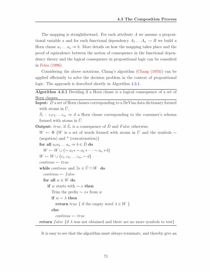
4.3 The Composition Process
The mapping is straightforward. For each attribute A we assume a proposi-
tional variable a and for each functional dependency A1 . . . An → B we build a
Horn clause a1 . . . an ⇒ b. More details on how the mapping takes place and the
proof of equivalence between the notion of consequence in the functional depen-
dency theory and the logical consequence in propositional logic can be consulted
in Felea (1996).
Considering the above notations, Chang’s algorithm (Chang (1976)) can be
applied efficiently to solve the decision problem in the context of propositional
logic. The approach is described shortly in Algorithm 4.3.1.
Algorithm 4.3.1 Deciding if a Horn clause is a logical consequence of a set of
Horn clauses.Input: D a set of Horn clauses corresponding to a DeVisa data dictionary formed
with atoms in U ,
Sr : c1c2 . . . cm ⇒ d a Horn clause corresponding to the consumer’s schema
formed with atoms in U .
Output: true, if Sr is a consequence of D and False otherwise.
W ← Φ {W is a set of words formed with atoms in U and the symbols ∼(negation) and * (concatenation)}for all a1a2 . . . an ⇒ b ∈ D do
W ←W ∪ {∼ a1∗ ∼ a2 ∗ · · · ∼ an ∗ b}W ← W ∪ {c1, c2, . . . cm,∼ d}continue← true
while continue and ∃x ∈ U ∩W do
continue← false
for all w ∈W do
if w starts with ∼ x then
Trim the prefix ∼ x∗ from w
if w = λ then
return true { if the empty word λ ∈W }else
continue← true
return false {if λ was not obtained and there are no more symbols to test}
It is easy to see that the algorithm must always terminate, and thereby give an
71
4.3 The Composition Process
answer. That this algorithm gives the correct answer is an immediate consequence
of Changs theorem on Horn clauses (Chang & Lee (1973)) and Fagin’s equivalence
theorem (Fagin (1977)). The algorithm gives a correct answer in linear time in
the number of atoms in the clauses in the data dictionary.
In the implicit composition scenario the PMQL engine builds the sequenced
model in order to score on the dataset provided in the scoring request. It then
stores the model back in the repository for future use.
4.3.2 Explicit Composition
Explicit Composition is when a DM consumer explicitly specifies in its goal that a
composition is desired. The composition query usually includes the models to be
composed, the composition method and a validation data set. DeVisa identifies
the specified models and checks them for compatibility. If all the prerequisites for
the composition are fulfilled then a new valid model is returned to the user/stored
in the repository.
An explicit composition scenario occurs when a consumer wants to make the
best out of several heterogeneous models in DeVisa complying to the same mining
schema. In this case it provides a composition goal (query) that be expressed as
(MSpec, R), where MSpec has the same signification as in the scoring goal. R
is a relation containing classified instances defined on the same schema as the
models satisfying MSpec. R is called a validation set.
DeVisa uses a stacking approach (see 3.4.1 ) to train a meta-learner ϕ based
on the outcomes of the existing DeVisa base models, i.e the models that satisfy
MSpec and the relation R provided by the consumer. Let’s assume that the
base schema is S = (U, P ), where U = {A1, A2, . . . , An} and the base classifiers
ϕ1, ϕ2, . . . , ϕm : dom(A1)× dom(A2)× · · · × dom(An)→ dom(C) , where C ∈ U .
The meta-learner is a simple decision tree τ : dom(C)m → dom(C) (by default
DeVisa uses ID3), since the main work is done by the base classifiers. The
outcome is another classifier ϕ : dom(A1)×dom(A2)×· · ·×dom(An)→ dom(C),
as depicted in Figure 4.3.
This approach has the advantage of fitting the model to the consumer needs
and the particularities of its own data. For this reason this method can be seen
72

4.3 The Composition Process
DeVisa
Consumer
c
...
Figure 4.3: Explicit composition of models in DeVisa through a stacking ap-
proach.
as a model customization instance as well.
Note that it is possible that the base models are based on composition as
well since DeVisa can store composed models. Nevertheless, they are treated
atomically.
Model composition is allowed only within a common data dictionary. Intu-
itively, a data dictionary refers to a strict domain. In the absence of a reference to
a data dictionary in the consumer’s goal, the same results can be achieved upon
the availability of a common domain ontology, composed of concepts describing
the domain in different abstraction levels, into which URLs are mapped. How-
ever, there are cases in which separate pre-existing ontologies are used. DeVisa
does not address this aspect. In the Semantic Web SW community this is an
intense matter of research and much valuable work is done in the domains of
ontology alignment, meaning negotiation or ontology elicitation and application.
These techniques are over-viewed in Hepp et al. (2008) and Davies et al. (2006).
73

Chapter 5
Semantic Integration and the
Implications in DeVisa
5.1 Basic Terminology
Semantic integration has been a long-standing challenge for the database commu-
nity and has nowadays become a prominent area of database research in multiple
areas, such as artificial intelligence, e-commerce, bioinformatics, semantic web
and ubiquitous computing. The volume of data available online and within or-
ganizations has been increasing exponentially in the latest years. The recent
growth of the Web 2.0 has fueled the spread of data sharing web applications
and created the need of semantic integration of the shared heterogeneous and
independent data.
In the Semantic Web (SW), data is annotated using ontologies. Concepts
(or classes) in ontologies give meaning to data on the Web. Because ontologies
are shared specifications, the same ontologies can be used for the annotation
of multiple data sources, like Web pages, collections of XML documents, rela-
tional databases, etc. As was argued in Uschold (2000), it is very hard to create
standard ontologies because the standardization of a terminology is not feasible,
especially in an inter-organizational context. As a result there are many different
heterogeneous ontologies on the Semantic Web and in order to enable interoper-
ability between applications on the Semantic Web, mediation is required between
different representations (ontologies, schemas) of knowledge in the same domain.
74

5.1 Basic Terminology
So, schemas and ontologies have a couple of properties in common: provide a
vocabulary of terms that describes a domain of interest and constrain the meaning
of terms used in the vocabulary.
There are a number of terms that have been coined in the context of medi-
ation: matching, mapping, alignment, relating, merging. With a few differences,
they are trying to achieve the same main objective: bringing two or more on-
tologies/schemas into mutual agreement, by reconciling the differences between
them.
In de Bruijn et al. (2006), a more exact hierarchical classification is made. At
the high level we can distinguish two types of mediation: mapping and merging.
With ontology mapping, the correspondences between two ontologies are stored
separately from the ontologies and thus are not part of the ontologies themselves.
The correspondences can be used for, for example, querying heterogeneous knowl-
edge bases using a common interface or transforming data between different rep-
resentations. The (semi-)automated discovery of such correspondences is called
ontology alignment.
More formally, a schema/ontology mapping M is a declarative specification
of the semantic overlap between two ontologies OS and OT . This mapping can
be one-way (injective) or two-way (bijective). In an injective mapping we specify
how to express terms in OT using terms from OS in a way that is not easily
invertible.
When performing ontology merging, a new ontology is created which is the
union of the source ontologies. The merged ontology captures all the knowledge
from the original ontologies. The challenge in ontology merging is to ensure that
all correspondences and differences between the ontologies are reflected in the
merged ontology.
Both mapping and merging have as input a specification of similarities be-
tween the schemas/ontologies, which is called the matching process, detailed in
5.3.
75

5.2 Applications of Semantic Integration
5.2 Applications of Semantic Integration
There is a considerable number of specific problems that have driven research in
the field of schema alignment (Doan & Halevy (2005)). One of them is schema
integration, or integrating multiple schemas into a global one. The integration
process requires establishing semantic correspondence - matches - between the
component schemas, and then using the matches to merge schema elements (Pot-
tinger & Bernstein (2003)).
In an artificial intelligence setting, this is the problem of integrating indepen-
dently developed ontologies into a single ontology.
Another very popular topic is data translation in between database applica-
tions, which is a critical step in building data warehouses and performing data
mining activities. Here data originating from different sources must be trans-
formed to conform to a single target schema to enable further data analytical
processing (Miller et al. (2000)). Given a data source, one approach (Bernstein &
Rahm (2000)) to creating appropriate transformations is to start by finding those
elements of the source that are also present in the warehouse -match operation.
After an initial mapping is created, the detailed semantics of each source element
are examined and transformations that reconcile those semantics with those of
the target are created.
Another important class of applications is data integration ((Garcia-Molina
et al. (1997))). Such an application translates a user query on a global schema,
called mediated schema, to a set of queries applied on local underlying schemas
where the data resides. The queries are executed using wrapper systems attached
to the data sources, and the results are combined and translated to conform to
the mediated schema.
There are two approaches to specify the mapping between the mediated
schema and the source database schemas. One of them is to consider each of
the data sources to be a view over the (nonexistent) mediated schema. Formally
such an approach is called Local As View (LAV). The resulting architecture is
very flexible and scalable because it can easily absorb new data sources in the
system. Adding a new data source affects only the respective wrapper. In return,
query processing is more difficult because the query undergoes a radical process
76

5.2 Applications of Semantic Integration
of rewriting. It is possible that a query on the global schema cannot always be
translated on a specific local schema and incomplete answers to client queries
can occur. This happens because the number of tuples that can be expressed on
the global schema is larger than the one in the sources. On the other side, the
Global As View (GAV) approach considers the global schema to be a view on
each of the data source schemas. The latter approach has the advantage of the
simplicity of query processing, since the queries are expressed in a common view
on the sources. The drawback concerns scalability of such a system, because each
time a new data source is added, the mediated schema might need to be modified
to incorporate the new added source schema. This modification cascades to the
potential clients of the system, since the queries that are normally issued on the
mediated schema have to be rewritten. So this approach is suitable for systems
in which the source databases are not likely to suffer changes.
Another class of applications is the peer management applications, that allow
users (peers) to query and retrieve each other’s data. We encounter here an
extension of a mediated schema (Aberer (2003)), allowing to create semantic
correspondences between each pair of peers.
An important tool that benefits from semantic integration is the field of record
linkage, proposed in Dunn (1946). It refers to the task of finding entries that refer
to the same entity in two or more files. Record linkage is an appropriate technique
when data sets that do not have a unique database key in common need to be
joined. A data set that have been through record linkage is said to be linked. The
most popular approach is Probabilistic Record Linkage (Jaro (1995)). It can be
used to improve data holdings, data collection, quality assessment, dissemination
of information, duplicate removal. Important areas of application are: medical
practice and research and historical data archives (Winkler (1999), Jaro (1995)).
Record linkage is a useful tool when performing data mining tasks, where the
data originated from different sources or different organizations.
Recently an important application area that needs ontology mediation has
developed - Semantic Web Services (Fensel et al. (2007)). In general, it cannot
be assumed that the requester and the provider of a service use the same termi-
nology in their communication and thus mediation is required in order to enable
communication between heterogeneous business partners. It is subject to intense
77
5.3 Strategies in Achieving Schema and Ontology Mapping
research in the context of achieving the Semantic Web desiderates. One of the
promising fields of application of ontologies in Semantic Web (SW, Lee et al.
(2001)) is the integration of information from differently organized sources, e.g to
interpret data from one source under the schema of another, or to realize unified
querying and reasoning over both information sources.
5.3 Strategies in Achieving Schema and Ontol-
ogy Mapping
We define matching as the process of discovering similarities between two source
schemas or ontologies. The result of a matching operation is a specification of
similarities between them. The matching is done through application of the
Match operator - defined in Rahm & Bernstein (2001), which takes two schemas
(or ontologies) as input and produces a mapping between elements of the two
schemas that correspond semantically to each other. Any schema matching or
ontology matching algorithm - called matcher - can be used to implement the
Match operator.
There are many different algorithms which implement the Match operator.
These algorithms can be generally classified along several dimensions.
• Schema types: relational, XML, entity-relationship (ER), OO, IDL etc;
• Metadata representation: XML schema, graph, ER, relational, OO etc;
• Syntactic or semantic matching. The syntactic matches take into account
different string matches techniques, such as prefix, suffix, longest common
substring, string metrics. One important syntactic method for ontology
alignment is the comparison of class and property names of ontologies us-
ing string distance metrics. Today quite a number of such metrics exist
in literature, such as the Levenshtein distance, LCS (longest common sub-
string) distance, Needleman-Wunsch distance, etc. The semantic techniques
take the word senses into account establishing lexical relationships between
entities (Miller (1995),Wor (2006)).
78
5.3 Strategies in Achieving Schema and Ontology Mapping
• Rule or learning based techniques. The rule-based matching technique acts
at the syntactic level and consists of applying rules created manually to re-
alize the schema matching. In general, the rules exploit schema information
such as element names, data types, structures, number of subelements, and
integrity constraints. The source schema is compared with the target one,
and each component in the source schema is matched with a corresponding
component in the target schema.
The rule based matching techniques operate only on schemas and do not
analyze the data instances. Therefore they are inexpensive from the time
and space perspective and are domain independent, although they can be
tailored to fit a certain domain.
The rule-based approach has two major drawbacks, both related to the
lack of information on the data instances themselves. The data instances
can encapsulate a lot of meta-information, such as format, frequencies of
words in certain attributes extreme values, mean, distribution of the values
etc. The first drawback is the fact that such valuable information cannot be
used in the matching process. Another drawback is that rule-based methods
cannot exploit previous matching efforts to assist in the current ones. Thus
we can say that systems that rely solely on rule-based techniques are statical
and cannot learn from the past to improve the accuracy of the results.
The above reasons have motivated the development of learning based schema
matching. The solutions have considered a variety of learning techniques
and exploited both schema and data information. Most of the actual sys-
tems are hybrid in the sense that they analyze the schema from both syntac-
tic and semantic angles and the data instances to establish a more accurate
discovery of similarities.
• Match granularity: element-level, structure-level, relationship-level. etc.
Match can be performed for individual schema elements, such as attributes,
or for combinations of elements, such as complex schema structures. In the
second case the schemas/ontologies are viewed as graph-like structures con-
taining terms and their inter-relationships and techniques based on bounded
path matching, super/sub-concept rules, children, leaves are applied.
79

5.3 Strategies in Achieving Schema and Ontology Mapping
• Match cardinality: 1:1, n:1, 1:n, n:m. The match result may connect one
element of a schema to one or more elements of the other schema. This can
reflect at the instance level as well.
• Schema level or instance level. Schema-level matchers only consider schema
information, not instance data. The available information includes the usual
properties of schema elements, such as name, description, data type, rela-
tionship types (part-of, is-a, etc.), constraints, and schema structure. In
general, a matcher will find multiple match candidates. For each candi-
date, a degree of similarity in the range of [0, 1] is usually calculated and
the best candidates are those for whom the degree of similarity exceeds a
certain threshold. Instance-level exploit the data instances, which give a
precise characterization of the actual contents of schema elements and can
give important insight into their meaning. This is especially true when
useful schema information is limited.
• Need for auxiliary information. There are matchers that rely not only on
the input schemas but also on other metadata, such as dictionaries, global
schemas, previous matching decisions and user input.
• The level at which the alignment works: schema, data instances;
• Simple, hybrid or composite. Hybrid matchers directly combine several
matching approaches to determine match candidates based on multiple
criteria or information sources (e.g syntactic and semantic). A composite
matcher combines the results of several independently executed matchers,
including hybrid matchers, which tends to be more flexible then the hybrid
matchers.
• Need for manual input: human intensive ranging to fully automatic. Defines
the extent in which the user is involved in the matching process. Ideally, any
schema mapping tool should function with as less as possible input from the
user and ask only for absolutely necessary feedback. In Yan et al. (2001)
this issue is tackled by defining a framework that uses data examples as
the basis for understanding and refining declarative schema mappings. The
80

5.3 Strategies in Achieving Schema and Ontology Mapping
higher the degree of autonomy of the matcher, the lower the number of user
interactions and vice-versa. It is difficult to achieve a generic solution that is
adaptable to different application domains (although the approach could be
controlled by tuning parameters). Alternatively, a user can directly select
the matchers to be executed, their execution order and how to combine
their results. Such a manual approach is easier to implement and leaves
more control to the user.
In Rahm & Bernstein (2001), Sun & Rose (2003), Doan & Halevy (2005),
Predoiu et al. (2005) and Davies et al. (2006) surveys containing different strate-
gies to schema/ontology are presented matching and comparative analyses are
performed based on a pre-established set of features. To summarize, the taxon-
omy of the distinguishing properties for the schema/ontology matching problem
is presented in Figure 5.1.
5.3.1 Overview of the Existing Approaches
Early work such as TranScm system (Milo & Zohar (1998)) employed very simple
rules such as: two schema elements map to each other if they have the same
names (or synonyms) and the same number of sub-elements. The schemas are
represented in labeled graphs, the edges being labeled with the relationships.
The relationship properties (name, optionality, cardinality, transferability) are
associated with the nodes. The algorithm performs an element level, 1:1 match,
based on plugable rules.
In DIKE (Palopoli et al. (2000)) system the similarity between two schema
elements is computed through the similarity of the characteristics of the elements
and the similarity of the related elements. It attempts to automatically determine
new synonym and inclusion (is-a, hypernym) relationships between objects of
different entity-relationship schemas. The algorithms are based on a set of user
specified synonym, homonym, and inclusion properties labeled with a numerical
confidence factor (between 0 and 1). In order to (probabilistically) derive new
synonyms and homonyms and the associated plausibility factors, the authors
perform a pairwise comparison of objects in the input schemas by considering
81

5.3 Strategies in Achieving Schema and Ontology Mapping
Figure 5.1: A taxonomy of the dimensions that characterize the schema/ontology
matching strategies (Rahm & Bernstein (2001)).
the similarity properties of their related objects (i.e., their attributes and the is-a
and other relationships the objects participate in).
The ARTEMIS system (Castano & Antonellis (1999)) operates on a hybrid
relational-OO model that includes the name, data types, and cardinalities of at-
tributes and target object types of attributes that refer to other objects. First it
computes affinities in the range 0 to 1 between attributes, which is a match-like
step. It then completes the schema integration by clustering attributes based
on those affinities and then constructing views based on the clusters. The algo-
rithm computes matches by a weighted sum of name and data type affinity and
structural affinity. Name affinity is based on generic and domain-specific the-
sauri, where each association of two names is a synonym, hypernym, or general
relationship, with a fixed affinity for each type of association. Data type affin-
ity is based on a generic table of data type compatibilities. Structural affinity
82

5.3 Strategies in Achieving Schema and Ontology Mapping
of two entities is based on the similarity of relationships emanating from those
entities. ARTEMIS is used as a component within a heterogeneous database me-
diator, called MOMIS (Bergamaschi et al. (2001)). MOMIS prescribes the use of
a global merged ontology for the integration of data sources.
Cupid(L.Madhavan et al. (2001)) is a hybrid matcher based on both element-
and structure-level matching. It is intended to be generic across data models
and has been applied to XML and relational examples. It uses auxiliary informa-
tion sources for synonyms, abbreviations, and acronyms. Like DIKE, each entry
in these auxiliary sources include a plausibility factor in the [0, 1] range. The
algorithm has three phases. The first phase does linguistic element-level match-
ing and employs rules that categorize elements based on names, data types, and
domains. It parses compound element names into tokens based on delimiters,
categorizes them based on their data types and linguistic content, and then cal-
culates a linguistic similarity coefficient between data type and linguistic content
compatible pairs of names based on substring matching and auxiliary sources.
The second phase transforms the original schema into a tree and then does a
bottom-up structure matching, resulting in a structural similarity between pairs
of element. This transformation encodes referential constraints into structures
that can be matched just like other structures (making Cupid constraint-based).
The similarity of two elements at the root of structures is based on their linguistic
similarity and the similarity of their leaf sets. If the similarity exceeds a threshold,
then their leaf set similarity is incremented. The focus on leaf sets is based on
the assumption that much of the information content is represented in leaves and
that leaves have less variation between schemas than internal structure. Phase
two concludes by calculating a weighted mean of linguistic and structural simi-
larity of pairs of elements. The third phase uses that weighted mean to decide
on a mapping.
The LSD (Learning Source Descriptions) system uses machine-learning tech-
niques to match a new data source against a previously determined global schema,
producing a 1:1 element-level mapping Doan et al. (2001). It both matches names
at the schema level and trains several instance-based matchers to discover char-
acteristic instance patterns and matching rules that can then be applied to match
other data sources to the global schema. Given a new data source, each matcher
83

5.3 Strategies in Achieving Schema and Ontology Mapping
determines a list of match candidates and a global matcher is used to merge the
lists into a combined list of match candidates for each schema element. LSD has
also been extended to consider user-supplied domain constraints on the global
schema to filter out the previously determined match candidates for improving
match accuracy.
The SemInt system (Li et al. (2000)) is a hybrid matcher that uses a neural-
network learning approach. For each schema element it builds a ”matching sig-
nature” based on matching criterions, such as attribute specifications (e.g, data
types, scale, the existence of constraints) and statistics of data content (e.g., max-
imum, minimum, average, and variance). Each signature can be seen as a point
in the N-dimensional space, so the Euclidean distance can be used as a degree
of similarity between elements and generating match candidates. Then it uses
neural networks to determine match candidates. It first clusters the attributes in
the first schema based on the Euclidean distance and then assigns each attribute
in the second schema to a cluster based on a neural network trained with the
already built cluster centers.
The iMAP (Dhamankar et al. (2004)) matches the schemas of two sources by
analyzing the description of objects that are found in both sources. It takes a
more domain-oriented approach by utilizing matchers that are designed to detect
and deal with specific types of data, such as phone numbers. It also has an
approach to searching for schema translations for numerical data using equation
discovery.
Perkowitz & Etzioni (1995) investigates the problem of automatically learning
declarative models of information sources available on the Internet and proposes a
system named ILA that learns the meaning of external information by explaining
it in terms of internal categories.
Ryutaro et al. (2001) proposes a concept alignment method for concept hier-
archies as a solution to this problem, and construct a system called HICAL to
evaluate the performance of the method. The proposed method can be used to in-
duce align rules for concept hierarchies and classify information into appropriate
categories within another concept hierarchy.
Giunchiglia et al. (2004) presents a 4 step semantic structural approach, called
S-Match. It assumes that the conceptual models (schemas, ontologies) are repre-
84

5.3 Strategies in Achieving Schema and Ontology Mapping
sented as trees. It is based on the notions of concept of a label, which denotes the
set of documents (data instances) that one would classify under a label it encodes,
and concept at a node, which denotes the set of documents (data instances) that
one would classify under a node, given that it has a certain label and that it is in
a certain position in a tree. The algorithm takes as input two schemas and com-
putes as output a set of mapping elements in four macro steps: (1) for all labels
in the two trees, compute concepts of labels; (2) for all nodes in the two trees,
compute concepts at nodes; (3) for all pairs of labels in the two trees, compute
semantic relations (e.g., equivalence, more/less general) among the corresponding
concepts at labels; (4) for all pairs of nodes in two trees, compute relations among
the concepts at nodes.
The GLUE system, presented in Doan et al. (2004), applies machine learning
techniques to semi-automatically create semantic mappings. Since taxonomies are
the central components of ontologies, the system finds the correspondences among
the taxonomies of two given ontologies. So for each concept in a taxonomy, it finds
the most similar concept in the other. The similarity is defined in terms of joint
probability distribution of the concepts involved. It also uses domain constraints
and heuristics, such as ”Two nodes are likely to match if their neighbors also
match”. GLUE uses a probabilistic model to combine results of different learners,
which makes it a composite matcher.
The COMA++ system (Aumueller et al. (2005)) utilizes a a composite ap-
proach to combine different match algorithms, supporting schemas and ontologies,
e.g. W3C XML Schema(Sperberg-McQueen & Thompson (2008)) and OWL(OWL
(2007)). COMA++ is characterized by: the utilization of shared taxonomies, the
application of the different match strategies including various forms of reusing
previously determined match results and the fragment-based matching, which
decomposes a large match problem into smaller problems.
Curino et al. (2007) introduces an ontology mapping and integration tool
called X-SOM, which combines several matching techniques by means of a neural
network, performing semi-automatic resolution of inconsistencies.
85

5.4 Implications of the Schema Mapping in DeVisa
5.4 Implications of the Schema Mapping in De-
Visa
Schema matching problem also impacts the scoring process in DeVisa (4.2).
Briefly, it occurs when a consumer application would like to score a given data
set having no knowledge if DeVisa contains a data dictionary (or schema) that
matches the schema of its data set. When solving the consumer’s goal containing
a laxly specified target DeVisa model, the scoring engine (3.2) is performing a
schema matching to identify an appropriate model or models to score on. During
this process, it needs to iterate over the existing DeVisa data dictionaries and
attempt to perform a mapping.
Furthermore, a query written in terms of the consumers application termi-
nology needs to be rewritten using the terms in DeVisa data dictionary - query
rewriting (3.3.2.2).
The final purpose of mapping in DeVisa is the consumer’s data instances
transformation according to the DeVisa mining schema, so that a mining model
can be applied. The mapping should be reversible, in the sense that the answer
to a goal should reflect the consumer’s schema.
DeVisa is designed to serve random consumer applications through web ser-
vices. Therefore the schema mapping process should function without manual
intervention. In these circumstances the system should have the possibility to de-
cide, under configurable parameters (degree of similarity, optimistic/pessimistic
approach), if to apply a certain mapping or not. A manual validation process can
be performed at consumer’s site after a scoring answer based on a set of matches
is returned.
In DeVisa schemas correspond to data dictionaries. In a data dictionary one
or more mining schemas can be defined, which are considered to be elements
in a data dictionary. A mining schema corresponds to a single mining model
and specifies additional properties for the attributes that are used in the mining
model. Examples of such properties are usage type, importance, missing values
treatment etc. A detailed formal description of the DeVisa data model can be
consulted in 4.1 and an overview on mining schemas is presented in 2.5.1.2. These
86

5.4 Implications of the Schema Mapping in DeVisa
properties are used in the schema matching resolution in DeVisa. For instance,
the matching should give higher priority to higher importance attributes.
Data dictionaries are often correlated to taxonomies that describe hierarchi-
cal parent-child relationships between the categorical fields. In the context of a
mining schema, additional properties for each field can be specified. These prop-
erties specify the manner in which the mining model manipulated the specific
field: dealing with missing or inconsistent values etc.
Moreover, the transformation dictionary can specify rules and procedures to
transform individual or group of fields into derived fields that are used in the min-
ing model instead of the original fields. The transformations can be applied either
at single row level or multiple row level (aggregation functions). Its role is to map
user data to values that are easier to use in the mining model. The transformation
dictionary broadens the spectrum of match candidates, since the consumer data
might be expressed using also derived fields. Therefore the matching strategy can
be considerably improved if it takes into account potential matches induced by
the transformation functions.
On the other side one can imagine the case in only a subset consumer’s at-
tributes are used in the prediction process, namely the maximal subset that can
be mapped to a DeVisa data dictionary and for which an adequate mining schema
can be deduced (i.e it either exists or can be composed as shown in 4.3). Never-
theless the degree of coverage of the consumer’s set of attributes is a configurable
parameter (i.e support).
One of the main characteristics of the DeVisa system is that it does not store
the data the models were built on, but it is meant to enable model and predic-
tion interchange between applications. Therefore some of the schema matching
strategies (especially instance based strategies) that employ learning techniques
cannot be applied. Nevertheless the consumer’s data that needs to be scored on
is available and can be analyzed. On the other side a model expressed in PMML
can contain univariate statistics on each of the fields used in the mining model
(see 2.5.1). Therefore a technique that builds a ”matching signature” in the man-
ner presented in Li et al. (2000) could be applied for certain data dictionaries.
To improve the efficiency of the matching during the model discovery phase of
the scoring procedure the preprocessing should be done offline. In this way, each
87

5.4 Implications of the Schema Mapping in DeVisa
schema element has the internal matching representation stored along with the
corresponding data dictionaries.
Furthermore, or at the moment the data dictionaries are uploaded in the
system, a match process is triggered between the newly added data dictionary
and the set of data dictionaries existing in the system. This process can identify
similarities between the schema elements and sets up incrementally a integrated
network of concepts. The algorithm is described in 3.2.1. This setup contributes
to the efficiency of the online schema matching and also builds up the prerequisites
for the model composition (4.3).
Another aspect worth mentioning is the type of relations that are established
during the match process. In DeVisa we are not necessarily interested in mode
complex relations like in most of the systems, such as: equivalence (=), more
general (⊆), disjointness (⊥), but moreover in degrees of similarity. The question
is: can a DeVisa model be applied on this specific attribute? So relations like
generalization and specialization are likely to be mapped in lower degrees of
similarity.
In summary, the distinguishing properties of the DeVisa conceptual model
compared to other schema matching input configurations are:
• entities are not explicitly defined. Intuitively, a mining schema (and, respec-
tively, a model) refers to a specific entity, but it is possible that multiple
mining schemas refer to the same entity;
• lack of structural constraints which are normally present in a relational
database schema (e.g primary or foreign keys);
• a data dictionary may refer a specific taxonomy; several data dictionaries
may refer the same taxonomy;
• optional univariate statistics at the field level;
• optional textual description of the data dictionaries, or for the individual
fields;
• optional transformation dictionary;
88

5.5 Schema Matching Approach in DeVisa
• the type of relationships that are targeted reduces to degrees of similarity
Provided the context and the requirements presented above, the scoring pro-
cess in DeVisa is a novel problem whose resolution involves strategies used in
schema and ontology mapping, mediation and query rewriting. The schema
matching strategy used in DeVisa is described formally in 5.5.
5.5 Schema Matching Approach in DeVisa
In DeVisa schema matching is necessary during the model discovery phase in the
scoring or search process, namely in the match schema case (see 4.2.1.2). Given
a consumer’s schema Sr, the matching process means identifying a set of optimal
match functions. The optimal match functions for a consumer’s schema is defined
in 4.11.
This section provides an algorithmic approach for calculating the set of op-
timal match functions for a given consumer’s schema. It uses the Global Data
Dictionary, which is part of the Metadata Catalog (see 3.2).
Prior to describing the schema matching algorithm , we need to define several
concepts.
Definition 5.1 Given a consumer’s schema Sr = (Ur, Pr) and Dg a DeVisa
GDD, c, s ∈ [0, 1], we define a global matching as a partial function m : Ur → 2Ug
with support s and confidence c so that both of the following are true:
1. Ag ∈ m(Ar) if simArAg≥ c
2. |{Ar|m(Ar) 6= ∅}| ≥ s|Ur|
The maximum number of candidate global matches is:
(
|Ur|⌈s|Ur|⌉
)
2|Ug| +
(
|Ur|⌈s|Ur|⌉+ 1
)
2|Ug| + · · ·+(
|Ur||Ur|
)
2|Ug|
=2|Ug|
((
|Ur|⌈s|Ur|⌉
)
+
(
|Ur|⌈s|Ur|⌉+ 1
)
+ · · ·+(
|Ur||Ur|
))
=2|Ur|O(2|Ug|−1) (5.1)
=O(2|Ur |+|Ug|−1) (5.2)
89
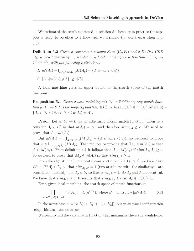
5.5 Schema Matching Approach in DeVisa
We estimated the result expressed in relation 5.1 because in practice the sup-
port s tends to be close to 1 (however, we assumed the worst case when it is
0.5).
Definition 5.2 Given a consumer’s schema Sr = (Ur, Pr) and a DeVisa GDD
D}, a global matching m, we define a local matching as a function m′ : Ur →2U1∪U2...Un, with the following restrictions:
1. m′(Ar) =⋃
Ag∈m(Ar)(M(Ag)− {A|simArA < c)}
2. |{Ar|m(Ar) 6= ∅}| ≥ s|Ur|
A local matching gives an upper bound to the search space of the match
functions.
Proposition 5.1 Given a local matching m′ : Ur → 2U1∪U2...Un, any match func-
tion µ : Ur → U has the property that ∀Ar ∈ U ′r we have µ(Ar) ∈ m′(Ar) where U ′
r =
{Ar ∈ Ur s.t ∃A ∈ U s.t µ(Ar) = A}.
Proof. Let µ : Ur → U be an arbitrarily chosen match function. Then let’s
consider Ar ∈ U ′r so that µ(Ar) = A , and therefore simArA ≥ c. We need to
prove that A ∈ m′(Ar).
But m′(Ar) =⋃
Ag∈m(Ar)(M(Ag) − {A|simArA < c)}, so we need to prove
that A ∈ ⋃
Ag∈m(Ar)(M(Ag). That reduces to proving that ∃Ag ∈ m(Ar) so that
A ∈ M(Ag). From definition 4.1 it follows that A ∈ M(Ag) if sim(Ag, A) ≥ c.
So we need to prove that ∃Ag ∈ m(Ar) so that simAg,A ≥ c.
From the algorithm of incremental construction of GDD (3.2.1), we know that
∀A′ ∈ U∃A′g ∈ Ug so that simA′
g ,A′ = 1 (two attributes with the similarity 1 are
considered identical). Let Ag ∈ Ug so that simAgA = 1. So Ag and A are identical.
We know that simArA ≥ c. It results that simArAg≥ c, so Ag ∈ m(Ar). �
For a given local matching, the search space of match functions is:
∏
Ar∈Ur,m′(Ar)6=∅
|m′(Ar)| = O(n′|Ur |), where n′ = maxAr∈Ur|m′(Ar)|. (5.3)
In the worst case n′ = O(|U1|+ |U2|+ · · ·+ |Un|), but in an usual configuration
setup this case cannot occur.
We need to find the valid match function that maximizes the actual confidence.
90

5.5 Schema Matching Approach in DeVisa
Definition 5.3 A local matching m′ is valid if a valid match function can be
obtained from it.
In another words, a local matching is valid if it can map the fields in the
consumer’s schema into fields within the same DeVisa dictionary.
At a first glance the problem that we need to solve of finding the optimal valid
match function can be reformulated using graphs. So, given a weighted tripartite
graph G = (Ur, Ug, U1 ∪ U2 . . . Un, m′ ∪M ′), where m′ = {(Ar, Ag) so that Ag ∈m(Ar)} and M ′ = {(Ag, A) so that A ∈ M(Ag)}, each edge in m′ ∪ M ′ being
annotated with values from sim we are interested finding a set of paths with
exactly 2 edges having maximal overall confidence from vertices in in Ur to vertices
in only one of U1, U2, . . . , Un. An instance of this problem is depicted in figure
5.2.
Ur
Ug
U = U1 U U2
Figure 5.2: An example of a valid matching using tripartite graph representation.
The set of bold paths represents a valid local match function. The two data
dictionaries are represented in squares and diamonds respectively.
We are going to further reduce the problem to a simpler one that can be
modeled using bipartite graphs. In order to do this we need to transform the
global matching to a local matching.
The algorithm for determining a local matching in DeVisa given a consumer’s
schema is depicted in 5.5.1.
In the first phase of the algorithm a global matching m is calculated. m is
represented as an association table that maps each attribute Ar in the consumer’s
schema with a set of candidate match attributes in the global data dictionary Dg.
In the second phase m is transformed into a local matching that maps Ur
to attributes in the local data dictionaries using the pre-calculated M function,
which is part of the global data dictionary. If necessary, the similarity values need
to be recalculated (getSim function). The GDD plays an important role because
91

5.5 Schema Matching Approach in DeVisa
Algorithm 5.5.1 Finding a a valid applicable local matching for the consumer’s
schema.Input: Sr = (Ur, Pr) the consumer’s schema
Dg = (Ug, M) the global data dictionary as a view on the data dictionaries
D1, D2, . . . , Dn in DeVisa
sim a memoization table of the similarity measures between Dg and
D1, D2, . . . , Dn and between Sr and Dg respectively.
Output: An valid local match m, if it exists
null, otherwise.
for all Ar ∈ Ur do
m(Ar)← ∅for all Ar ∈ Ur do
for all Ag ∈ Ug do
5: if simArAg> c then
m(Ar)← m(Ar) ∪ {Ag}for all Ar ∈ Ur do
for all Ag ∈ m(Ar) do
for all A ∈M(Ag) do
10: if simArAg= 1 or simAgA = 1 then
m(Ar)← m(Ar) ∪ {A}else
if getSim(Ar, A) ≥ c then
m(Ar)← m(Ar) ∪ {A}15: m(Ar)← m(Ar)− {Ag}
if m(getPredictedAttribute(Sr)) = ∅ then
return ∅if |⋃Ar∈Ur
µ(Ar)| < s|Ur| then
return ∅20: support = |Ur|
for Ar ∈ Ur do
if m(Ar) = ∅ then
support← support− 1
if support < s|Ur| then
25: return ∅return m
92

5.5 Schema Matching Approach in DeVisa
it reduces substantially the search for match candidates to a smaller number of
attributes.
After computing m, the algorithm tests if the attribute that needs to be
predicted has a match in DeVisa (getPredictedAttribute function returns the
attribute for which the predicted property is true). If not, a derivable match
function can never be produced out of the local matching. Then it checks if the
support is preserved (both in Ur as in m(Ur)) and only if it is it validates the
local matching.
So at the end of this phase m maps each Ar to a set of attributes in the DeVisa
data dictionaries. The attributes are spread across all the data dictionaries in
DeVisa. At this moment we don’t know if the local matching is valid, i.e if some
valid match functions can be determined.
The two phases of the algorithm reduce in polynomial time the above men-
tioned problem to a constrained form of the assignment problem in weighted
bipartite graphs.
In its classical form, the assignment problem requires finding a minimum
weight subset of edges so that for any vertex in the graph, it is incident to at
most one of the edges in the subset (such a subset is called matching). The
assignment problem is tightly related to the bipartite matching problem, which
requires finding the maximum cardinality independent set of edges in a bipartite
unweighted graph (any two edges in the set don’t share any common vertex).
This class of problems can be solved efficiently using a more generic class
of algorithms using flow networks. The flow network based algorithms are the
preferred way to model different problems because there are straightforward im-
plementations that are guaranteed to run in time proportional to a polynomial
in the size of the network.
A flow network is a weighted network where we interpret edge weights as
capacities. We refer to a network with a designated source s and a designated
sink t as an st-network. The objective is to compute a second set of edge weights,
bounded by the capacities, which called flow. The max-flow problem requires
finding a flow in a st-network such that no other flow from s to t has larger value.
An effective approach to solving max-flow problems was developed by Ford
and Fulkerson (Ford & Fulkerson (1956), Ford & Fulkerson (1962)). It is a generic
93
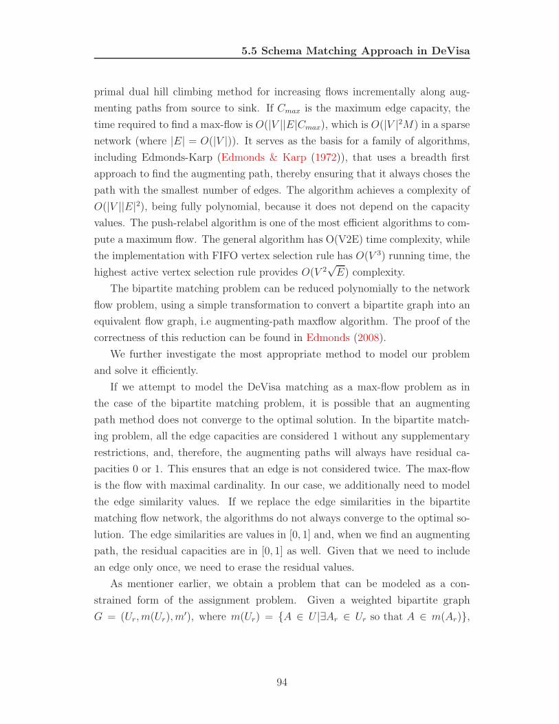
5.5 Schema Matching Approach in DeVisa
primal dual hill climbing method for increasing flows incrementally along aug-
menting paths from source to sink. If Cmax is the maximum edge capacity, the
time required to find a max-flow is O(|V ||E|Cmax), which is O(|V |2M) in a sparse
network (where |E| = O(|V |)). It serves as the basis for a family of algorithms,
including Edmonds-Karp (Edmonds & Karp (1972)), that uses a breadth first
approach to find the augmenting path, thereby ensuring that it always choses the
path with the smallest number of edges. The algorithm achieves a complexity of
O(|V ||E|2), being fully polynomial, because it does not depend on the capacity
values. The push-relabel algorithm is one of the most efficient algorithms to com-
pute a maximum flow. The general algorithm has O(V2E) time complexity, while
the implementation with FIFO vertex selection rule has O(V 3) running time, the
highest active vertex selection rule provides O(V 2√
E) complexity.
The bipartite matching problem can be reduced polynomially to the network
flow problem, using a simple transformation to convert a bipartite graph into an
equivalent flow graph, i.e augmenting-path maxflow algorithm. The proof of the
correctness of this reduction can be found in Edmonds (2008).
We further investigate the most appropriate method to model our problem
and solve it efficiently.
If we attempt to model the DeVisa matching as a max-flow problem as in
the case of the bipartite matching problem, it is possible that an augmenting
path method does not converge to the optimal solution. In the bipartite match-
ing problem, all the edge capacities are considered 1 without any supplementary
restrictions, and, therefore, the augmenting paths will always have residual ca-
pacities 0 or 1. This ensures that an edge is not considered twice. The max-flow
is the flow with maximal cardinality. In our case, we additionally need to model
the edge similarity values. If we replace the edge similarities in the bipartite
matching flow network, the algorithms do not always converge to the optimal so-
lution. The edge similarities are values in [0, 1] and, when we find an augmenting
path, the residual capacities are in [0, 1] as well. Given that we need to include
an edge only once, we need to erase the residual values.
As mentioner earlier, we obtain a problem that can be modeled as a con-
strained form of the assignment problem. Given a weighted bipartite graph
G = (Ur, m(Ur), m′), where m(Ur) = {A ∈ U |∃Ar ∈ Ur so that A ∈ m(Ar)},
94

5.5 Schema Matching Approach in DeVisa
m′ = {(Ar, A), A ∈ m(Ar)} is the directed edge set corresponding to the local
matching m obtained in the second phase of the algorithm 5.5.1 and sim is the
similarity table, containing the similarity values for the edges in m′ . We need to
find a maximal actual confidence matching µ so that all the vertices in µ(Ur) inci-
dent with edges in the matching are part one and only of U1, U2, . . . , Un (validity
condition) and form a derivable mining schema.
There are several standalone approaches to solve the assignment problem. Us-
ing the Kuhn-Munkres (Hungarian) combinatorial optimization algorithm (Munkres
(1957)) it can be resolved in O(|U |3) (U being the vertex set). The algorithm
works by increasing the number of zeros in the matrix and searching for a set of
starred zeros, one in every row and column. Zeros are primed, starred, or neither
during the algorithm. If there are insufficient zeros a quick Gaussian elimination
adds more. If there are not enough starred zeros, the primed zeros are starred
and the starred zeros primed. Primed zeros are zeros in a column without any
more zeros, which, because they are in the same row as another zero were not
starred. The Hungarian algorithm cannot be used in DeVisa due to the fact that
it is tightly coupled with the assignment problem configuration and therefore
supplementary restrictions cannot be incorporated.
A more generalized flow network model is the mincost−maxflow model, in
which the edges have both capacities and costs. The flow cost of an edge in a
flow network with edge costs is the product of that edge’s flow and cost. The
cost of a flow is the sum of the flow costs of that flow’s edges. The problem is
to find a maxflow such that no other maxflow has lower cost. In DeVisa we are
moreover interested in a variation of the problem, in which the flow that needs
to be calculated has maximum confidence (as opposed to cost) and maximum
cardinality (flow). We will further call it max-flow max-confidence.
To model this problem as the max-flow max-confidence problem, we first need
to do some prior transformation of the graph, which is described in algorithm
5.5.2. We will also observe some useful properties related to the particularity of
the obtained network that can improve the performance of the provided algo-
rithms.
Basically this transformation adds for each data dictionary Di a source vertex
si (and edges from si to each attribute in Di) and a sink node t (with edges from
95

5.5 Schema Matching Approach in DeVisa
Algorithm 5.5.2 Transformation of the DeVisa weighted bipartite graph into a
multiple source single sink flow network.
Input: G = (Ur, m(Ur), m′) and sim defined earlier
Output: Gf = (Uf , mf) a flow network with sources {s1, . . . sn} and sink t
Gf ← GT
Uf ← Uf ∪ {s1, . . . sn, t}for all Ar ∈ Ur do
if m(Ar) 6= ∅ then
5: mf ← mf ∪ {(Ar, t)}simArt ← 0
else
Uf ← Uf − {Ar}for all Ui ⊆ Ur do
10: for all A ∈ Ui do
mf ← mf ∪ {(si, A)}simsiA ← 0
for all (u, v) ∈ mf do
capuv ← 1
15: for all Ar ∈ Ur do
if importance(Ar) = null then
if usage(Ar) = active or usage(Ar) = predicted then
importance(Ar)← 1
else
20: importance(Ar)← 0
for all A ∈ m(Ar) do
simArA ← simArA ∗ importance(Ar)
return Gf
96

5.5 Schema Matching Approach in DeVisa
each vertex in Ur) to t. For each of the new edges, the similarity value is considered
0 and the capacity is 1 for all the edges in the network. For each attribute in Ur the
importance of the attribute is taken into consideration. The importance measures
the correlation between the respective attribute and the predictive attribute. In
PMML the specification of the importance property is optional, whereas the
usage type is active by default. Predicted fields and active fields are the most
important, while supplementary fields have moreover explanatory purpose and
are not used by the algorithm. Therefore they do not count in the matching
process. In the transformation algorithm we adjusted the similarity measure so
that higher importance fields count more in the computation of the confidence.
All the attributes in Ur that cannot match any attribute in U are eliminated.
The newly built network is called Gf .
Having this transformation we redefine our purpose as finding the max-flow
with max-confidence that starts in one of the sources. If there are several such
flows, we would like to keep them all. Furthermore, for each of the identified
flows we need to check the derivability condition (defined in 4.12). In case the
derivability is not satisfied, we want to have the option of trying the next ”best”
flow, i.e the one with max-confidence from the remaining flows.
For each of the sources si in Gf we consider the subgraph Gif induced by all
the vertices accessible from si. The algorithm 5.5.3 builds a set of max-flows for
each of Gif sit-networks and choses the ones with the highest confidence for which
the derivability condition is fulfilled.
It uses the priority queue PQMatch to store all the max-flows in Gif . The
reason why we retain all the max-flows is that, if the top priority max-flow does
not satisfy the derivability property, then it is eliminated from the queue and the
next one is tested. When a max-flow that satisfies the derivability property as
well is encountered, the others are dropped and the search continues with Gi+1f .
Figure 5.3 depicts an example of such a subgraph Gfi , where edges are an-
notated with (capacity, similarity) and the match functions µ1, µ2, µ3 that are
some of the potential solutions (match functions).
97

5.5 Schema Matching Approach in DeVisa
Algorithm 5.5.3 Applying the max-confidence max-flow algorithm for the in-
dividual data dictionaries and selecting the one that is both derivable and has
maximum confidence.Input: Gf = (Uf , mf), sim and cap as defined in algorithm 5.5.2
Output: A set of max-flows F so that ∀f ∈ F we have conf(f) = maxf ′conf(f ′)
where conf(µ) = 1|Ur|
∑
(u,v)∈µ simuv
cmax ← 0
F ← ∅for all si ∈ {s1, . . . , sn} do
U ir ← {ur ∈ Ur|∃u ∈ Ui so that (ur, u) ∈ mf}
Gif ← ({si, t} ∪ Ui ∪ U i
r, mif)
PQMatch← getMaxF lows(Gif )
while PQMatch 6= ∅ do
(f, c)← dequeue(PQMatch)
if isDerrivable(f, Di) then
if c > cmax then
cmax ← c
F ← {f}else
if c = cmax then
F ← F ∪ {f}else
break
return F
98

5.5 Schema Matching Approach in DeVisa
(1,0.8)
si
t
(1,0.7)
(1,0)
A1 A2 A3
Ar1
Ar3
(1,0)
(1,0)
Ar2
(1,0) (1,0)
(1,0)
(1,0.9)
0.8
0.8
A1A2
Ar1 A
r2
A3
Ar3
0.9
0.8 0.7
A1A2
Ar1 A
r2
0.80.9
A1 A3
Ar1
Ar2
support(μ2)=0.66
support(μ1)=0.66
support(μ3)=1.00
...
conf(μ1)=0.50
conf(μ2)=0.56
conf(μ3)=0.80
A3
Ar3
Ar3
A2
(a) (b)
(1,0.9)(1,0.8)
Figure 5.3: Examples of match functions (b) and the corresponding flow-network
conform to algorithm 5.5.3 (a). The match function µ3 has maximum confidence
and will be chosen.
Proposition 5.2 In the residual network Gir = (U i
r, mir) of any max-flow in the
network Gif built in algorithm 5.5.3, we have:
∀u, v ∈ U ir if (u, v) ∈ mi
r then (v, u) /∈ mir.
Proof. It results from the topology of the network Gif and from the construc-
tion of the residual network Gir.
Let f be the max-flow from which Gif was built. We have two situations.
First (u, v) ∈ f . Then flowuv = 1, resuv = 0 and resuv = 1 (results from the
procedure augment). This means that (u, v) /∈ mir and (v, u) ∈ mi
r. Secondly,
(u, v) /∈ f . Then flowuv = 0, resuv = 1 and resuv = 0 (results from the procedure
augment). This means that (u, v) ∈ mir and (v, u) /∈ mi
r. �
Proposition 5.3 In Gir = (U i
r, mir) we have
1. deg+(t) = deg−(si).
2. ∃tAArsi a path from t to si.
99

5.5 Schema Matching Approach in DeVisa
Proof. Both properties result directly from the flow conservation property
and from the construction of Gir based on a non-empty flow. �
Proposition 5.4 In the residual network Gir = (U i
r, mir) we have:
1. if (Ar, A) ∈ mir, then (t, Ar) ∈ mi
r and (A, si) ∈ mir
2. if (t, Ar) ∈ mir, then ∃!A ∈ Ui so that (Ar, A) ∈ mi
r and (A, si) ∈ mir
3. if (A, si) ∈ mir, then ∃!Ar ∈ Ur so that (Ar, A) ∈ mi
r and (t, Ar) ∈ mir
Proof. If (Ar, A) ∈ mir, it corresponds to the edge (A, Ar) ∈ µ, the flow on
which Gir is based on. It follows that there is a an entire corresponding path from
t to si in Gir, so (t, Ar) ∈ mi
r and (A, si) ∈ mir. The other two properties can be
proven in a similar fashion.�
Proposition 5.5
if (A, Ar) ∈ mir, then deg+(Ar) = 1 and deg−(A) = 1.
Proof. Let us prove that deg+(Ar) = 1. We have two exclusive possibilities:
(t, Ar) ∈ mir or (Ar, t) ∈ mi
r.
If (t, Ar) ∈ mir, then from property 5.4 it results that A is the unique attribute
so that (A, Ar) ∈ mir, so deg+(Ar) = 1.
If (Ar, t) ∈ mir then we know that deg+(Ar) ≥ 1. Let us assume that
deg+(Ar) > 1. Then ∃A′ ∈ Ui so that (Ar, A′) ∈ mi
r. Then from property
5.4 it follows that (t, Ar) ∈ mir, which conflicts with the hypothesis. Therefore
deg+(Ar) = 1.
Using a similar rationale we prove that deg−(A) = 1. �
The algorithm 5.5.4 builds a priority queue named PQMatch containing the
max-flows arranged in descending order of their confidence. The algorithm uses
the cycle canceling approach and it is based on the property that a max-flow is a
max-confidence maxflow if and only if its residual network contains no negative-
cost directed cycle (Sedgewick (2003)).
The cost of the cycle in the residual network is calculated as
cost(cycle) =∑
(u,v)∈cycle
costuv ∗ resuv.
100

5.5 Schema Matching Approach in DeVisa
where the costuv = 1 − simuv, for all the edges with strictly positive similarity.
For the others, cost is 0.
Algorithm 5.5.4 getMaxF lows(Gif)
Input: Gif = (U i
f , mif), a sit network, sim and cap as defined in algorithm 5.5.3
Output: PQMatch = {µ max-flow with max(|µ|)}, a priority queue containing
the max-flows in Gif , with the priority set by the value of the actual confidence.
PQMatch← ∅(f, c)← getMaxF low(Gi
f)
if deg+(si) < s ∗ |Ur| then
return ∅repeat
enqueue(PQMatch, (f, c))
cycle← getNegativeCycle(Gif , t)
if cycle 6= ∅ then
augment(f, cycle)
path← ∅while path 6= ∅ do
path← getAugmentingPath(Gif)
augment(Gif , path)
until cycle = ∅return PQMatch
procedure augment(G, P )
for all (u, v) ∈ P do
flowuv ← flowuv + 1
flowvu ← flowvu − 1
resuv ← resuv − 1
resvu ← resvu + 1
The algorithm starts with identifying a max-flow and then attempts to identify
a negative cost cycle in the residual network. If one is found the flow is saved
in the priority queue and then it is is augmented along the negative cycle. The
iteration continues until no more negative cost cycles can be found. It is possible
101

5.5 Schema Matching Approach in DeVisa
that, after augmenting along a negative cost cycle, a new augmenting path is
discovered. In this case the algorithm finds it by calling the function described
in 5.5.6 and augments the flow along it.
Proposition 5.6 The number of augmenting cycles needed in algorithm 5.5.4 is
O(|mif |).
Proof. We know that ∀(u, v) ∈ mif , 0 < costuv ≤ 1−c. Let us consider the worst
case when in the initial max-flow each edge has the maximum possible cost, which
is 1 − min(u,v)∈mifsimuv = 1 − c, where c is the tuning parameter representing
the confidence of the match function. So in the worst case the cost of the initial
max-flow is at most |Ur| ∗ (1− c).
Each augmentation along a negative cycle replaces at least one edge with at
least another edge with lower cost. We can only do O(mif ) such replacements. �
Proposition 5.7 In the residual network Gir = (U i
r, mir), if deg+(si) > 0 then
there is at least one cycle that includes si.
Proof. deg+(si) > 0, then ∃A ∈ Ui so that (si, A) ∈ mir. We constructed Gf
in algorithm 5.5.2 such as all the attributes in Uf can be matched with at least
another attribute. So, ∃Ar ∈ Ur so that either (A, Ar) ∈ mir or (Ar, A) ∈ mi
r.
From property 5.2, it results that only one of the two holds.
If (Ar, A) ∈ mir, then, from property 5.4, it results that (A, s) ∈ mi
r, which
conflicts with (s, A) ∈ mir, according to the proposition 5.2.
It results that (A, Ar) ∈ mir. From property 5.5 it results that deg+(Ar) = 1.
Therefore we further have two mutual exclusive possibilities: (Ar, t) ∈ mir, or
(t, Ar) ∈ mir.
If (Ar, t) ∈ mir, then siAArt is a path from si to t. Using the property 5.4, it
results that it exists a cycle that includes si.
If (t, Ar) ∈ mir, then, from property 5.4 it results that ∃A′ 6= A so that
(Ar, A′) ∈ mi
r and (A′, si) ∈ mir. We obtained the cycle siAArA
′si that obviously
includes si. �
Proposition 5.8 Given Gif = (U i
f , mif ) the network built in 5.5.3, for any cycle
in the residual network, it is accessible from t.
102

5.5 Schema Matching Approach in DeVisa
Proof. Let C be a cycle in Gif . From property 5.2 it results that C has a
length of at least 4 edges.
If C includes si then, based on property 5.3, it follows immediately that C is
accessible from t.
If C does not include si, then C either includes t, or not. If it includes, then
we are finished.
If not, let us consider C = A1rA
1 . . . AlrA
lA1r, where l ≥ 4. Because of
(Ajr, Aj) ∈ mi
r and property 5.4 it results that (t, Ajr) ∈ mi
r, ∀j = 1 . . . l so C
is accessible from t. �
Based on the result given by the property 5.8, we can apply the cycle iden-
tification algorithm depicted in 5.5.5 starting from t to detect and identify a
negative cost cycle. In the first phase it builds the shortest paths from t to
the other vertices. It maintains a FIFO queue of all vertices for which relax-
ing along an outgoing edge could be effective. The main loop takes a vertex off
the queue, relaxes along all its edges, and updates the queue as appropriate. It
uses a sentinel value to separate vertices that changed on the previous pass from
those that change in the current one. The loop terminates after |U if | passes. In
the second phase it tries to apply another relaxation. If this would be effective,
this means that we discovered an edge in a negative cost cycle. Then the algo-
rithm loops until it completely discovers the cycle and returns it. The second
phase is done in O(|Ufi |). The cycle detection algorithm runs in O(|Uf
i | ∗ |mfi |)
computational time.
The cycle identification algorithm is based on an adapted version of Bellman-
Ford algorithm (Bellman (1958)) Bellman-Ford is a label correcting algorithm
that computes single-source shortest paths in a weighted digraph, where some of
the edge weights may be negative.
The algorithm 5.5.7 uses an augmenting path approach to find a max-flow.
It starts with zero flow everywhere and then increases the flow along any path
from source si to sink t with no full forward edges or empty backward edges,
continuing until there are no such paths in the network. The implementation
uses the shortest augmenting path, and therefore the search for an augmenting
path amounts to breadth-first search (BFS) in the residual network, as it can be
seen in algorithm 5.5.6. The time needed to find an augmenting path is O(|mif |).
103

5.5 Schema Matching Approach in DeVisa
Algorithm 5.5.5 getNegativeCycle(Gif , t)
for all v ∈ Ui do
pathcosttv ←∞pathcostt ← 0
Q← {t, sentinel}while Q 6= ∅ do
u← poll(Q)
if u = sentinel then
level← level + 1
if level ≥ |U ir| − 1 then
return ∅enqueue(Q, sentinel)
for w ∈ Ufi so that resuw 6= 0 do
if pathcostw ≥ pathcostu + costuw ∗ resuw then
pathcostw ← pathcostu + costuw ∗ resuw
parentw ← u
for all v ∈ U ir do
if pathcostv > pathcostparentv + costparentvv ∗ resparentvv then
cycle← {(parentv, v)}u← parentv
while u 6= v do
cycle← cycle ∪ {(parentu, u)}u← parentu
return cycle
return ∅
104
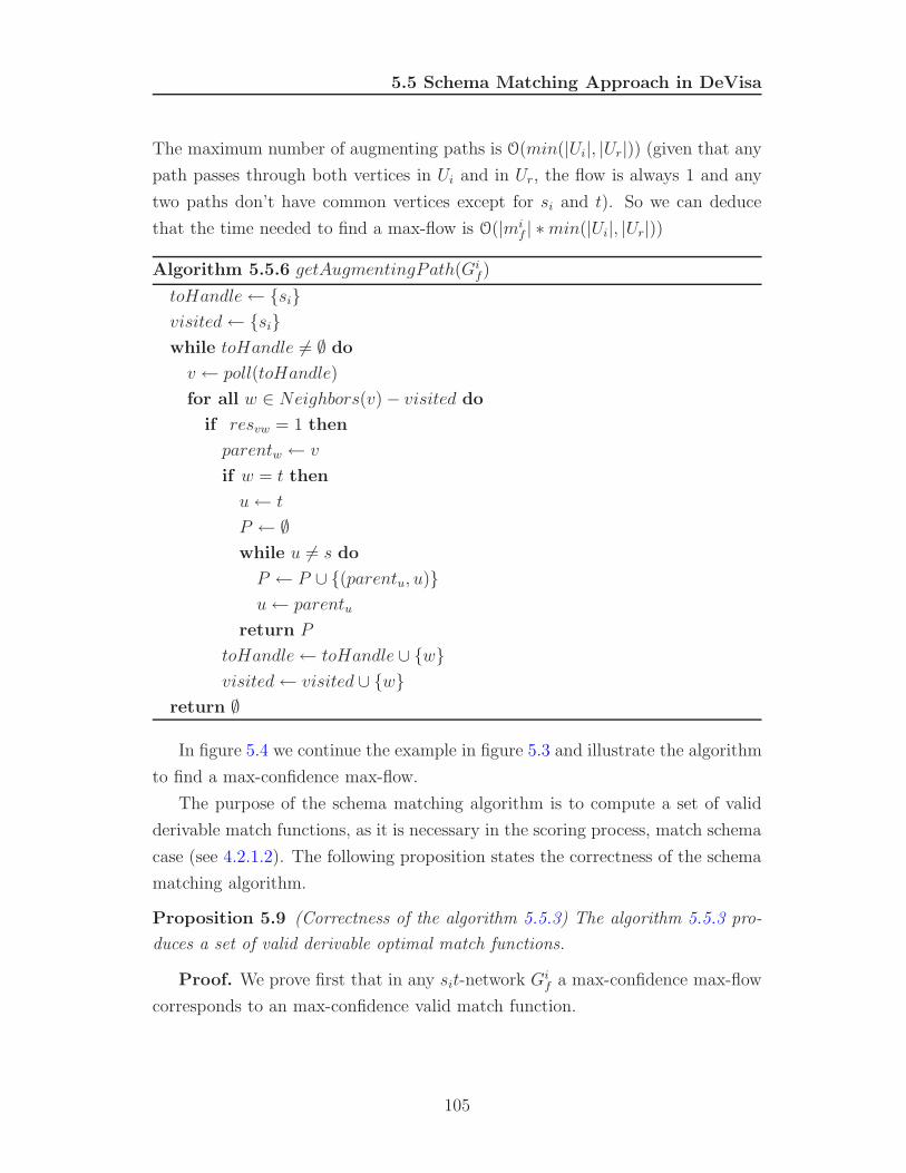
5.5 Schema Matching Approach in DeVisa
The maximum number of augmenting paths is O(min(|Ui|, |Ur|)) (given that any
path passes through both vertices in Ui and in Ur, the flow is always 1 and any
two paths don’t have common vertices except for si and t). So we can deduce
that the time needed to find a max-flow is O(|mif | ∗min(|Ui|, |Ur|))
Algorithm 5.5.6 getAugmentingPath(Gif)
toHandle← {si}visited← {si}while toHandle 6= ∅ do
v ← poll(toHandle)
for all w ∈ Neighbors(v)− visited do
if resvw = 1 then
parentw ← v
if w = t then
u← t
P ← ∅while u 6= s do
P ← P ∪ {(parentu, u)}u← parentu
return P
toHandle← toHandle ∪ {w}visited← visited ∪ {w}
return ∅
In figure 5.4 we continue the example in figure 5.3 and illustrate the algorithm
to find a max-confidence max-flow.
The purpose of the schema matching algorithm is to compute a set of valid
derivable match functions, as it is necessary in the scoring process, match schema
case (see 4.2.1.2). The following proposition states the correctness of the schema
matching algorithm.
Proposition 5.9 (Correctness of the algorithm 5.5.3) The algorithm 5.5.3 pro-
duces a set of valid derivable optimal match functions.
Proof. We prove first that in any sit-network Gif a max-confidence max-flow
corresponds to an max-confidence valid match function.
105

5.5 Schema Matching Approach in DeVisa
Algorithm 5.5.7 getMaxF low(Gif)
Input: Gif = (U i
f , mif), a sit network, sim and cap as defined in algorithm 5.5.3
Output: µ max-flow with max(|µ|)µ← Φ
for all (u, v) ∈ mif do
flowuv ← 0
flowvu ← 0
resvu ← 1
resuv ← 0
if simuv > 0 then
costuv ← 1− simuv
costvu ← simuv − 1
else
costuv ← 0
costvu ← 0
repeat
P ← getAugmentingPath(Gif)
if P 6= ∅ then
µ← µ ∪ P
augment(µ, P )
until P 6= ∅return µmax
procedure augment(Gif , P )
for all (u, v) ∈ P do
flowuv ← flowuv + 1
flowvu ← flowvu − 1
resuv ← resuv − 1
resvu ← resvu + 1
106

5.5 Schema Matching Approach in DeVisa
A1A2
Ar1 A
r2
A3
Ar3
(a)
si
t
(1,-0.2)
A1A2
Ar1 A
r2
A3
Ar3
si
t
(1,-0.3)
(1,0)
(1,0)
(1,0)
(1,0)
(1,0)
(1,0.1)
(1,0.1) (1,0.2)
(1,0)
A1A2
Ar1
Ar2
A3
Ar3
si
t
(1,-0.2)
A1A2
Ar1 A
r2
A3
Ar3
si
t
(1,0.3)
(1,0)
(1,0)
(1,0)
(1,0)
(1,0)
(1,0.1)
(1,-0.1) (1,0.2)
(1,0)
A1A2
Ar1
Ar2
A3
Ar3
si
t
(1,-0.2)
A1A2
Ar1 A
r2
A3
Ar3
si
t
(1,0.3)
(1,0)
(1,0)
(1,0)
(1,0)
(1,0)
(1,-0.1)
(1,-0.1) (1,0.2)
(1,0)
(b) (c)
Figure 5.4: The sequence of max-flows and their corresponding residual networks.
The negative cost cycles and augmenting paths are depicted in bold.
So, a valid match function is a bijection µ : Ur → Ui so that s ∗ |Ur| ≥ |µ(Ur)|and sim(Ar, µ(Ar)) ≥ c.
The algorithm 5.5.4 produces a set of max-flows organized in a heap where
the max-flow with the maximum confidence has the maximum priority.
The algorithm 5.5.3 checks the derivability condition on the max-flows in
descending order and stops at the max-flow with the max-confidence for which
the condition holds.
Let f be the top-priority max-flow for which the derivability holds. We define
µ : Ur → Ui so that µ(Ar) = A iff (A, Ar) ∈ f . µ is a bijection (results from the
construction of the flow), is valid (because the flow only uses attributes in Ui)
and it is optimal because the confidence is maximum. s ∗ |Ur| ≥ |µ(Ur)|, because
algorithm 5.5.4 rejects all the flows for which deg+(si) < s ∗ |Ur|. From here we
deduce that µ is the optimal derivable valid match function.
In conclusion a set of optimal match functions across all the data dictionaries
is built. �
Proposition 5.10 The algorithm needs O(|Ur|2 ∗ |U |3 + |Ur|3 ∗ |U |2) in the worst
case to calculate a set of optimal derivable match functions.
107
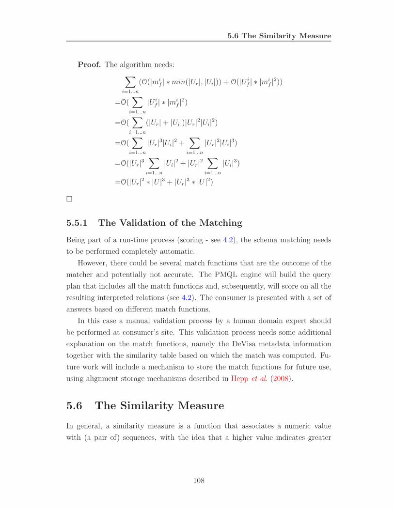
5.6 The Similarity Measure
Proof. The algorithm needs:
∑
i=1...n
(O(|mif | ∗min(|Ur|, |Ui|)) + O(|U i
f | ∗ |mif |2))
=O(∑
i=1...n
|U if | ∗ |mi
f |2)
=O(∑
i=1...n
(|Ur|+ |Ui|)|Ur|2|Ui|2)
=O(∑
i=1...n
|Ur|3|Ui|2 +∑
i=1...n
|Ur|2|Ui|3)
=O(|Ur|3∑
i=1...n
|Ui|2 + |Ur|2∑
i=1...n
|Ui|3)
=O(|Ur|2 ∗ |U |3 + |Ur|3 ∗ |U |2)
�
5.5.1 The Validation of the Matching
Being part of a run-time process (scoring - see 4.2), the schema matching needs
to be performed completely automatic.
However, there could be several match functions that are the outcome of the
matcher and potentially not accurate. The PMQL engine will build the query
plan that includes all the match functions and, subsequently, will score on all the
resulting interpreted relations (see 4.2). The consumer is presented with a set of
answers based on different match functions.
In this case a manual validation process by a human domain expert should
be performed at consumer’s site. This validation process needs some additional
explanation on the match functions, namely the DeVisa metadata information
together with the similarity table based on which the match was computed. Fu-
ture work will include a mechanism to store the match functions for future use,
using alignment storage mechanisms described in Hepp et al. (2008).
5.6 The Similarity Measure
In general, a similarity measure is a function that associates a numeric value
with (a pair of) sequences, with the idea that a higher value indicates greater
108
5.6 The Similarity Measure
similarity.
The similarity measure calculation algorithm in DeVisa is multi-faceted, being
able to adapt to take into consideration the available schema information. As
stated earlier much of the available metadata is optional and in the minimal case
the similarity measure needs to be calculated based only on schema based means.
DeVisa combines multiple available similarity criteria to achieve a final score,
which makes it a hybrid adaptive approach.
For instance the similarity between the global data dictionary and the DeVisa
data and transformation dictionaries utilizes merely schema based techniques,
but it also takes into account the the univariate statistics when they are available
(PMML standard specifies them as optional -see 2.5.1). Furthermore, during
scoring schema matching, the statistics on the consumer’s data instances need to
be calculated on the fly.
The only mandatory factor in calculating the similarity of elements in DeVisa
is the syntactic analysis of the terminology in the data dictionaries. Therefore
choosing an appropriate string metric is crucial in achieving good accuracy.
Today quite a lot of string metrics exist in literature and among others play
an important role in schema/ ontology mediation (Cohen et al. (2003)). A string
metric usually results in calculating a similarity or dissimilarity (distance) score
between two pairs of text strings. The most well known are the edit - or Levenstein
- distance (Levenstein (1966)), which counts the insertions and deletions needed to
match two strings, the sub-string distance which searches for the largest common
substring, the Needleman-Wunsch (Needleman & Wunsch (1970)) distance, which
assigns a different cost on the edit operations, the Smith-Waterman (Smith &
Waterman (1981)), which additionally uses an alphabet mapping to costs and
the Monge-Elkan (Monge & Elkan (1996)), which uses variable costs depending
on the substring gaps between the words, the Jaro-Winkler (Winkler (1999), Jaro
(1995)) similarity, which counts the common characters between two strings even
if they are misplaced by a short distance, the Q-Gram (Sutinen & Tarhio (1995)),
which counts the number of tri-grams shared between the two strings.
Taking into consideration features like the threshold (the value above which
two elements in a pair are considered identical), the cardinality of mappings,
109

5.6 The Similarity Measure
Stoilos et al. (2005) identifies the main characteristics of a string metric capable
of being used in schema/ontology mediation processes:
• Fast: Since ontologies are used in applications that demand processing in
real-time, like the semantic web or intelligent retrieval tasks, the complexity
of the string metric should be very low, leading to a fast matching procedure.
• Stable: This is the ability of a string metric to perform almost optimal
even if small diverges from the optimal threshold take place. Most of the
string metrics perform reasonably well if the threshold is optimized, but
the performance rapidly decrease if the value of the threshold is slightly
disturbed. There are methods that automatically adjust the threshold, as
opposed to the ones that use an a priori established threshold.
• Intelligent: When an ontology is compared to an irrelevant one, but with
which string resemblances occur, the metric should identify all the differ-
ences and provide correct results. It is very often that usual string metrics
fail to identify cases where two strings represent completely different con-
cepts but resemble a lot.
• Discriminating: In a 1 : 1 cardinality matching setup, which is a very
common requirement, if a field in one ontology is mapped with the same
similarity degree to several others in the other ontology, then it is very
probable that the matching algorithm fails to choose the right matching.
So it is desirable that a similarity metric rarely assigns the same similarity
degree when a string is compared to several others.
Given two mining schemas or data dictionaries, the DeVisa approach in cal-
culating the similarity performs the following steps:
Constraint Similarity. Two fields can map to each other only if the data
types are compatible. The compatibility can be checked using the XML Schema
types compatibility. A rougher data type categorization that is very relevant in
the statistic measures matching is categorical, ordinal and continuous fields. The
data type matching is realized by applying a set of a priori defined rules. So,
in case of categorical fields, the similarity is calculated as the ratio of common
110

5.6 The Similarity Measure
values of the total number of values in the domains of the two fields (Jacard
index).
if optype(A1) = categorical and optype(A2) = categorical then
DT (A1, A2) =|values(A1) ∩ values(A2)||values(A1) ∪ values(A2)|
Terminology criteria It uses the string metric described in Stoilos et al.
(2005) to compute a table of similarities between any pair of field names. PMML
allows both specification of a field name (an identifier relevant to PMML pro-
cessing) and a display name (which is normally displayed in user interfaces, but
irrelevant to PMML processing). The display name tends to have a higher de-
scriptive value, therefore we apply I-Sub on both names. This approach, called
Iterative-SubString (I-Sub), has been integrated in several popular ontology align-
ment and schema matching systems. It reveals good precision and recall when
in this context compared to other general purpose string metrics. Given two
attributes A1 and A2 the similarity between the two terms identifying the two
attributes is calculated as follows:
ISub(A1, A2) = Comm(A1, A2)−Diff(A1, A2) + Winkler(A1, A2)
where Comm(A1, A2) measures the commonality between the two fields and is
defined as:
Comm(A1, A2) =2∑
i len(LongestCommSubstri)
len(A1) + len(A2)
Au1 ← A1
Au2 ← A2
repeat
sub← LCSub(Au1 , A
u2)
if len(sub) ≥ 0 then
Au1 ← remove(Au
1 , sub)
Au2 ← remove(Au
2 , sub)
until len(sub) ≤ 0
111

5.6 The Similarity Measure
Diff(A1, A2) measures the dissimilarities based on the unmatched substrings Au1
and Au2 resulted from the previous procedure. It uses the Hamacher parametric
triangular norm (Hamacher et al. (1978)):
Diff(A1, A2) =len(Au
1)len(Au2)
p + (1− p)(len(Au1) + len(Au
2)− len(Au1)len(Au
2))
where p ∈ [0,∞) is a parameter that can adjust the importance of the difference
factor.
Winkler(A1, A2) quantifies the improvement of the result using the metric
described in Winkler (1999) and is defined as:
Winkler(A1, A2) = Jaro(A1, A2) + lpw(1− Jaro(A1, A2))
Jaro(A1, A2) =1
3(
m
len(A1)+
m
len(A2)+
m− t
m)
where l is the length of common prefix at the start of the attribute names
(up to a maximum of 4 characters), pw is a constant factor signifying how much
of the score is adjusted up when the names have common prefixes (standard
value is 0.1). m is the number of matching characters, and t is the number of
transpositions (matching characters which occur on different positions in the two
names).
The I-Sub string metric maps the similarity values in the interval [−1, 1]
and values above 0.4 signify high degree of similarity. For instance, the fields
microRNAStart and miRNAStart, both meaning the same concept, achieve a
degree of term similarity of 0.6607 when p = 0.6. In DeVisa we normalize the
ISub string metric to return values in [0, 1], i.e we consider:
NISub(A1, A2) =ISub(A1, A2) + 1
2
The complexity of the I-Sub string metric is polynomial to the size of the
input strings, satisfying the property of a fast metric.
Refinement.
1. Linguistic: Similarity is measured in terms of WordNet synsets (or senses),
namely structures containing sets of terms with synonymous meanings.
112
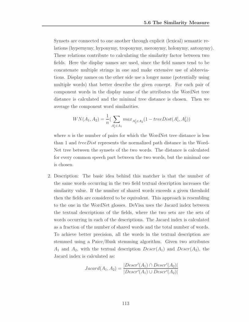
5.6 The Similarity Measure
Synsets are connected to one another through explicit (lexical) semantic re-
lations (hypernymy, hyponymy, troponymy, meronymy, holonymy, antonymy).
These relations contribute to calculating the similarity factor between two
fields. Here the display names are used, since the field names tend to be
concatenate multiple strings in one and make extensive use of abbrevia-
tions. Display names on the other side use a longer name (potentially using
multiple words) that better describe the given concept. For each pair of
component words in the display name of the attributes the WordNet tree
distance is calculated and the minimal tree distance is chosen. Then we
average the component word similarities.
WN(A1, A2) =1
n(
∑
Ai1∈A1
maxA
j2∈A2
(1− treeDist(Ai1, A
j2))
where n is the number of pairs for which the WordNet tree distance is less
than 1 and treeDist represents the normalized path distance in the Word-
Net tree between the synsets of the two words. The distance is calculated
for every common speech part between the two words, but the minimal one
is chosen.
2. Description: The basic idea behind this matcher is that the number of
the same words occurring in the two field textual description increases the
similarity value. If the number of shared words exceeds a given threshold
then the fields are considered to be equivalent. This approach is resembling
to the one in the WordNet glosses. DeVisa uses the Jacard index between
the textual descriptions of the fields, where the two sets are the sets of
words occurring in each of the descriptions. The Jacard index is calculated
as a fraction of the number of shared words and the total number of words.
To achieve better precision, all the words in the textual description are
stemmed using a Paice/Husk stemming algorithm. Given two attributes
A1 and A2, with the textual description Descr(A1) and Descr(A2), the
Jacard index is calculated as:
Jacard(A1, A2) =|Descr′(A1) ∩Descr′(A2)||Descr′(A1) ∪Descr′(A2)|
113
5.6 The Similarity Measure
where Descr′(A) is the set of stemmed words in A’s textual description.
For instance, considering again the attributes microRNAStart and miRNAStart,
with Descr(microRNAStart) =”The start gene position in the chromo-
some” and Descr(miRNAStart) =”The position in the chromosome where
the miRNA starts”, then
Jacard(microRNAStart, miRNAStart) = 0.6666.
Further work will refine the textual description similarity to behave in a
way similar to the gloss similarity in WordNet.
3. Statistical: The data instances statistical information (continuous or dis-
crete statistics) gives additional useful information for calculating the simi-
larity. It can be applied only if both data dictionaries provide this informa-
tion or the information can be inferred from the data instances themselves.
In the case of categorical/ordinal attributes we can use the modal value (the
most frequent value in the data set used to build the model). In the con-
sumer’s schema, this information can be easily deduced from the relation
that needs to be scored. Rules like the one hereunder can be used:
if (optype(A1) = categorical and optype(A2) = categorical
or optype(A1) = ordinal and optype(A2) = ordinal)
and modalV alue(A1) = modalV alue(A2) then
Stat(A1, A2)← 1
In the case of continuous attributes, for each of the attributes we build a
statistical signature that consists of a vector of N values corresponding to
each of the available statistical information. The signatures correspond to
points in the N -dimensional space. The signature for each of the attributes
is given by two vectors:
(a) uA, where uAi ∈ {0, 1}, i = 1 . . .N , where uAi marks if the respective
statistical index is present for the attribute A
(b)
signA = (invalid(A), missing(A), min(A), max(A),
mean(A), stdDev(A), median(A), interQuartileRange(A))
114

5.6 The Similarity Measure
where Invalid(A), missing(A) calculates the percentage of invalid/missing
values, mean(A) is the expected value, median(A) is the 50% quantile and
interQuartileRange(A) is calculated as 75% quantile −25% quantile.
The statistical distance between two attributes A1 and A2 is calculated as
the euclidean distance between the two signature vectors:
StatDist(A1, A2) =
√
∑
i=1,N
(signA1i − signA2i)2uA1iuA2i
To get to the statistical similarity score, we use the Shepard’s law (Shepard
(1987)):
Stat(A1, A2) = e−StatDist(A1,A2)
Structural. This step is performed when both data dictionaries are explained
through additional taxonomies. In this case a tree matching algorithm is per-
formed, taking into account the context in which each field is defined within the
taxonomy.
Steps 2 and 3 and 5.6 are optional, depending on the availability of the re-
spective information. The values obtained in the performed steps are aggregated
to produce the final similarity score.
The aggregation is achieved as follows. Three 6-dimensional vectors u, w and
s are calculated. The 6 dimensions represent the 6 match criteria presented above
(in this order).
1. u is a binary vector representing if a certain match criteria is present or not
in the matching strategy. The first two components of the vector will be
always 1. So ui ∈ {0, 1} and∑
i=1...6 ui ≥ 2.
2. w is a weight vector, where wi represents the importance that a match
criteria has in the matching strategy. Given that certain match criteria
could not be present, w should be adaptive to the availability of the match
criteria, so the following condition should hold:
∑
i=1...6
uiwi = 1.
115
5.6 The Similarity Measure
We start by considering equal weights to each of the present match criteria.
Based on experimental results, further improvement of the similarity mea-
sure will include probabilistic rule sets to adapt the weighting technique to
achieve better matching results.These rules will adjust w so that some of
the match criteria are assigned higher importance.
3. s is the vector of similarity scores achieved by applying each of the match
criteria. si ∈ [0, 1], the value of 1 corresponding to identical attributes. s
has the following structure:
s = (DT (A1, A2), NISub(A1, A2), WN(A1, A2),
Jacard(A1, A2), Stat(A1, A2), Struc(A1, A2))
Finally, the similarity between the fields is calculated as follows:
sim(A1, A2) =∑
i=1...6
uiwisi.
116

Chapter 6
Related Work
6.1 Online Scoring and Online Data Mining Ser-
vices
Another term for infrastructures providing resources/ services over the Internet
is the concept of a cloud. There are storage clouds (block and file based services),
data clouds (record-based, column-based, object-based services) and compute
clouds (computational services). Often these are layered to create a comput-
ing platform for developing cloud-based applications. Examples include Amazon
S3 (Ama (2008)), Google File System (Ghemawat et al. (2003)), BigTable and
MapReduce infrastructure (Dean & Ghemawat (2008)) etc.
The concept of knowledge as a service is a specialized sort of computing cloud.
In the context of automated knowledge elicitation from data sources, Krish-
naswamy et al. (2001) proposes two models of organization of the data mining
service providers and the interaction with their clients. The paper also describes
a XML based language for specifying data mining task requests and the services
of data mining service providers.
Due to the increasing usage of the web space as a platform (one of the main
goals of Web 2.0), there are many other proposals of data mining services available
on the web such as Chieh-Yuan Tsai (2005).
Grigorios Tsoumakas (2007) describes a web-based system for classifier shar-
ing and fusion named CSF/DC. It enables the sharing of classification models,
117

6.1 Online Scoring and Online Data Mining Services
by allowing the upload and download of such models expressed in PMML in the
system’s online classifier repository. It also enables the online fusion of classifi-
cation models located at distributed sites, which should be a priori registered in
the system using a Web form.
In Ali et al. (2005) web services are provided to implement data mining func-
tions like classifiers, clustering algorithms and association rules, and a workflow
engine for model composition.
WekaWS (*** (2007c), Talia et al. (2005)) is an initiative to provide the Weka
(Weka) data mining functions as WSRF - Web Service Resource Framework (***
(2004b)) web services. In such a way, distributed data mining tasks can be con-
currently executed on decentralized Grid nodes by exploiting data distribution
and improving application performance. In Weka4WS, the data mining algo-
rithms for classification, clustering and association rules can be also executed on
remote Grid resources. To enable remote invocation, all the data mining algo-
rithms provided by the Weka library are exposed as a Web Service, which can be
easily deployed on the available Grid nodes.
Grossman et al. (2004) introduces Open DMIX, an open source collection
of web services for the mining, integration, and exploration of remote and dis-
tributed data. Open DMIX is layered: the top layer provides templated data
mining and statistical algorithms, such as those defined by PMML. The mid-
dle layer provides access and integration of remote and distributed data. The
bottom layer provides specialized network protocols designed to work with large
distributed data sets over wide area networks. The clients interact with Open
DMIX servers using a version of web services designed for high performance ap-
plications (SOAP+).
Ferrucci et al. (2006) presents scenarios on how applications combining PMML
and UIMA framework can be built. The scenarios include using clustering or
probabilistic clustering PMML models to do text categorization (as opposed to
the bag of words approach), or processing XML tagged data to lower the classi-
fication level (from more specific to broader).
Grossman & Gu (2008) goes further and proposes a cloud-based infrastructure
(with storage and computing capabilities) that supports data mining applications.
118

6.2 PMML Scoring Engines
To facilitate the development of data mining and scoring-enabled applications,
APIs have been specified, such as Java Data Mining - JDM (*** (2005)), which
also includes web services extensions, i.e JDMWS.
6.2 PMML Scoring Engines
6.2.1 Augustus
Augustus (Chaves et al. (2006)) is an open source, PMML compliant system for
building and scoring statistical models that is designed to work data sets that are
too large to fit into memory. If data can fit into memory, then there are several
open source statistical systems available, including the R System (*** (2008b)).
Augustus is typically used to construct models and score data with models.
Augustus includes a dedicated application for creating, or producing, predictive
models rendered as PMML-compliant files. Scoring is accomplished by consum-
ing PMML-compliant files describing an appropriate model. Augustus provides
a dedicated application for scoring data with a class of models referred to as
Baseline Models. The typical Baseline model development and use cycle with
Augustus is as follows:
1. Identify suitable data with which to construct a new model.
2. Provide a model schema which proscribes the requirements for the model.
3. Run the Augustus producer to obtain a new model.
4. Run the Augustus consumer on new data to effect scoring.
In addition to the producer and consumer applications, Augustus is conceptu-
ally structured and provided with libraries which are relevant to the development
and use of predictve models. Broadly speaking, these consist of components that
address the use of PMML and components that are specific to Augustus. The
current version of Augustus consists of the following main components.
119

6.2 PMML Scoring Engines
1. A data management component called Unitable is part of the Augustus
kernel. A UniTable is broadly similar to a data frame in the R system. It
contains data fields arranged in columns, that may be of different types,
but all of which have the same number of rows.
2. Utilities for processing PMML files.
3. Components for shaping and transforming data. These components are also
part of the Augustus kernel.
4. Model specific components. Currently, Augustus supports baseline models
and tree-based models (DMG). These are collected together in the modellib
module.
5. Run time support. Augustus provides a general mechanism for reading data
into Augustus and writing data out of Augustus called anyreader and any-
writer, respectively. For example, anyreader can read data from a stream or
a file and put it into a common format for further processing by Augustus.
6. Miscellaneous tools. The Augustus distribution also includes a number of
auxiliary utilities, such as configuration utilities, utilities for working with
date and time etc. For example, there is a utility that will create a stub
PMML data schema based upon an analysis of a data file.
ADAPA is intrinsically a decision engine. It combines the power of predictive
analytics and business rules to facilitate the tasks of managing and designing
automated decisions systems. This essentially allows a consumer to deploy PMML
on the Amazon compute cloud (Ama (2008)). Rather than having to invest in
significant infrastructure to put models to work in production small and medium
sized organizations are now able to use the cloud and deploy them very cost
effectively. It uses browser based deployment, is standards based - web services
for run-time access, PMML for model design and JSR 73-JDM ((*** (2005)))
for run-time access to the engine. A consumer can use R, SPSS, SAS, or DB2
Intelligent Miner to build a model because these tools all support export into
PMML.
120
6.3 Comparison to DeVisa’s approach
It offers the computing cloud benefits - scalability, payment for the consump-
tion, reliability, as well as security. All the instances are managed through a
Control Center. One or more PMML models can be loaded in n instance, val-
idated against the PMML schema, interactively fix the potential problems and
deploy the model. Once deployed the model can be used as a web service (for
which WSDL is generated on the fly) or interactively. This allows the consumer
to upload and run data - either to score it or to match it against expected scores
for testing. Scored data can be downloaded in CSV format.
6.3 Comparison to DeVisa’s approach
Compared to the related work described in 6.1, DeVisa is particular in the fol-
lowing aspects:
• DeVisa does not store the data the models were built on, but only the
PMML models themselves;
• The DeVisa approach leverages the XML native storage and processing ca-
pabilities like indexing (structural, full text and range), query optimization,
inter-operation with the XML based family of languages and technologies;
• DeVisa defines a XML based query language - PMQL - used for interaction
with the DM consumers. PMQL is wrapped in a SOAP message, interpreted
within DeVisa and executed against the PMML repository;
• It provides a XML-based language for expressing the Metadata Catalog;
• DeVisa deals with schema integration aspects in the scoring process and
provides a 1 : 1 schema matching technique and an adaptive similarity
measure;
• Uses a functional dependency approach in verifying if a consumer’s schema
can be derived from the existing schemas in DeVisa;
• DeVisa allows online composition of prediction models either during the
scoring process or explicitly;
121

6.3 Comparison to DeVisa’s approach
• The interoperability with other applications (e.g consumers) is achieved
exclusively through the use of web services;
• DeVisa integrates a native XQuery library for processing PMML docu-
ments.
122
Chapter 7
Implementation Details
7.1 Overview of the Underlying Technologies
7.1.1 Native XML Database Systems
A native XML database is a database that defines a logical model for an XML doc-
ument and stores and retrieves documents according to that model. The model
should comprise at least elements, attributes, PCDATA, and document order.
Examples of such models are the XPath/XQuery data model (XDM (2007)), the
XML Infoset, the logical structure of documents and the way a document is ac-
cessed and manipulated defined by DOM (Hors et al. (2004)) and the events in
SAX (*** (2004a)), or the pull parsing model implied by StAX (*** (2007a)).
A XML database an XML document as its fundamental unit of (logical) stor-
age, just as a relational database has a row in a table as its fundamental unit
of (logical) storage. Is not required to have any particular underlying physi-
cal storage model. For example, it can be built on a relational, hierarchical, or
object-oriented database, or use a proprietary storage format such as indexed,
compressed files. An overview on the leading XML databases products can be
consulted in Gorea (2005a), as well as potential uses on XML native databases
in nowadays applications (Gorea (2005b)).
123

7.1 Overview of the Underlying Technologies
7.1.2 XQuery
XML(XML) is a versatile language, capable of describing the information con-
tent of diverse data sources including structured and semi-structured documents,
relational databases, and object repositories. A query language that uses the
structure of XML intelligently can express queries across all these kinds of data,
whether physically stored in XML or viewed as XML via middleware.
XQuery (XQuery) is a functional language designed for querying XML doc-
uments and it has become a W3C recommendation as of January 2007. The
language has the following distinctive properties: composition, closure, schema
conformance, XPath compatibility, completeness, conciseness, and static analy-
sis. XQuery complies to the requirement that an XML query language have both
a human-readable syntax and an XML-based syntax. XQuery operates on the
abstract, logical structure of an XML document, rather than its surface syntax.
This logical structure is known as the data model (XDM (2007)). Currently at
version 1.0, XQuery is an extension of XPath Version 2.0 (XPa (2007)).
It is flexible enough to query a broad spectrum of XML information sources,
including both databases and documents, which makes it suitable for wide use
in applications. DeVisa leverages the power of XQuery to implement efficient
processing of the PMML prediction models in the repository.
7.1.3 eXist
eXist (eXist, Meier (2002)) is a native XML database engine featuring efficient,
index-based XQuery processing, automatic indexing (structural, full-text, range),
extensions for full-text search, XUpdate support, XQuery update extensions and
tight integration with existing XML development tools. eXist provides basic
database functions such as storing and retrieving XML or binary resources and
XQuery/XPath querying via the XMLDB (*** (2003b)), XMLRPC(*** (2003a))
or SOAP (*** (2007b)) interfaces.
eXist supports calls to arbitrary Java methods from within XQuery. The bind-
ing mechanism follows the short-cut technique introduced by Saxon - a collection
of tools for processing XML documents (Kay (2008)).
124
7.1 Overview of the Underlying Technologies
eXist provides its own XQuery implementation, which is backed by an efficient
indexing scheme at the database core to support quick identification of structural
node relationships. The indexing scheme forms the very core of eXist and repre-
sents the basis of all efficient query processing in the database. The main purpose
of the indexing scheme is to allow a quick identification of structural relationships
between nodes. To determine the relationship between any pair of given nodes,
the nodes themselves don’t need to be loaded into main memory. This is a central
feature since loading nodes from persistent storage is in general an expensive op-
eration. For eXist, the information contained in the structural index is sufficient
to compute a wide-range of path expression.
This functionality is crucial for the implementation of DeVisa since it strongly
influences the performance of the PMQL engine while solving PMQL consumer
goals (3.3.2).
7.1.4 Web Services
Apache Axis2 Axi (2008) is the successor to the Apache Axis SOAP project,
providing a major improvement of the Web services core engine. Apache Axis2
provides a complete object model and a highly flexible modular architecture that
makes it easy to add functionality and support for new Web services-related
specifications and recommendations.
Axis2 enables performing the following tasks: send SOAP messages with or
without attachments, receive and process SOAP messages, retrieve the WSDL for
a service, create or utilize a REST-based Web service, create or utilize services
that take advantage of the WS-Security , WS-ReliableMessaging , WS-Addressing
, WS-Coordination , and WS-Atomic Transaction recommendations etc.
Being a clean and extensible open source Web services platform, it aims to
be the platform for the next generation of Web services and Service-Oriented
Architecture - SOA Erl (2005).
125
7.2 Current DeVisa Implementation
7.2 Current DeVisa Implementation
The main challenge in developing DeVisa is obviously the PMQL engine, that,
among others performs the PMML scoring. Compared to other scoring engines,
it is more flexible providing extra functionality such as: schema matching within
the scoring process and composition of prediction models. From a technology
perspective, it is able to natively process the PMML models using the XQuery
processing and indexing facilities offered by eXist.
At the time of writing this material, various parts of the DeVisa system are
under development and the current status of the implementation can be checked
out directly on the code repository on sourceforge.net (*** (2008c)). The details
of the implementation are presented hereunder.
From a functional design perspective, in Appendix C the main use cases of the
system are presented: scoring, explicit composition, search. The specifications
of the PMQL language expressed in XML Schema can be consulted in A. I also
designed the architecture of the system, which is described in various parts of
the present work. Also, the internal specification of the system is described, such
as the Metadata catalog, which is also specified in XML Schema (Appendix B).
The object model of the PMQL engine is also described in Appendix C.
Some of the horizontal cross-cutting aspects of the system are implemented:
web service front-end, a skeletal implementation of PMQL engine and its com-
ponents (annotator, rewriter, plan builder and plan executer) PMQL validation
against its schema, schema matching strategy described in section 5.5, as well as
the similarity measure described in 5.6.
The PMQL-LIB library includes an set of XQuery scoring functions - at this
moment only for tree models-that operates directly on the PMML models. These
functions are stored in the eXist XML database, like stored procedures.
DeVisa also includes a library that builds PMML based on Weka classifier
model classes using the Java Reflection API. It represents work in progress and
at the time of writing of this material it provides support only for several classi-
fication models (trees, naive bayes, rule set) and association rules. On the other
side, in the Weka Pentaho project, support for PMML in Weka is in progress at
126

7.2 Current DeVisa Implementation
the time of writing this material. This module is likely to be more comprehensive
and further supported along with future releases of the PMML specification.
In order to provide a proof of concept some of the DeVisa functions are devel-
oped also as Pentaho Data Integration plugins, as described in the concrete use
case presented in 8.5. These are the prediction voting component, the global data
dictionary or the schema matcher. These components are adapted to conform to
the metadata constraints present in the PDI data flows and hence are compatible
with the other PDI transformation steps. This offers the users the possibility
of development of complex data integration projects that include prediction and
decision support capabilities.
127
Chapter 8
Applications
8.1 DeVisa in a SOA
Service Oriented Architectures (or SOAs) are architectures meant to integrate
autonomous software applications based on the business processes that they ser-
vice. It is irrelevant whether the autonomous software applications are designed
to interact with one another (loosely coupling). This is achieved through a typical
property of a SOA, namely an Enterprise Server Bus (ESB). The ESB is in the
most basic form a layer in the SOA that routes XML messages from one software
component to another based on the content of the XML message. The routing
of the message, thus the description of the recipient(s) based on the values of an
xml schema, is defined in a message book, being part of the ESB. The ESB can
also perform transformation of data offered by the sender of an XML, before it
is offered to the intended recipient.
There are two ways of implementing a SOA: (1) an implementation of business
logic, data layer and user interfaces designed to interoperate with one another; (2)
an implementation that enables software applications to service business processes
without them being designed to interoperate with one another.
For the implementation of business logic that is designed to operate with one
another there is the pre-requisite that the interface of business logic and user
interface is done through XML, for instance through the use of web services. The
user interface will interact with one or more business logic components without
the user being aware of the back-end that is servicing him or her. The back-end
128

8.1 DeVisa in a SOA
ESB
Process
Enterprise
Database
UI
app 1
UI
app 2
UI
app 3
UI
app portal
Process
Process
xml
Figure 8.1: The General SOA Architecture.
processes will execute transactions on one database, either being one enterprise
database, distributed databases or a federated database. The routing of the
XML message from UI to a back-end component as well as between the back-end
component and the UI and/or database is done via the ESB based on the content
of the XML as mentioned above.
For the integration of applications that were not designed to interoperate with
one another the only thing that needs to be done is making sure that there is
an interface between the application and the ESB, either done through a generic
web service that most ESBs offer, or by developing a connector with the ESB.
This scenario is used most of the times when implementing SOAs and it is the
textbook example of the integration of loosely coupled applications. It is called
loosely coupled as the different applications have no interfaces with one another
(thus making it possible to replace applications very easily) but together service
a business process dictated by the way the XML schema through which they
communicate is agreed upon.
As the services in DeVisa are published as web services it is by default able
to service in a SOA as for instance a decision support component. The data
mining producers or consumers can be nodes in the SOA as well. The producers
should be able to communicate through PMML. The consumers should be able
to communicate through PMQL.
In Alboaie et al. (2008a) an SOA-based architecture of an e-health system is
presented, in which DeVIsa is integrated as a module to provide medical predic-
tion support. Additional details on the architecture on the mentioned e-Health
129

8.2 DeVisa as a Knowledge Repository for Learning Interface Agents
ESB
DM
producer
DM
consumer
DM
producer
xml
Database 1 Database 2
Database 3
DeVisa
Figure 8.2: Integration of DeVisa in a SOA architecture.
system can be consulted in Alboaie et al. (2008b).
8.2 DeVisa as a Knowledge Repository for Learn-
ing Interface Agents
An interface agent is a semi-intelligent, semi-autonomous computational system
which assists a user with a computer application. Such an agent is called a learn-
ing agent if it monitors and memorizes the user’s actions and preferences, discov-
ers regularities in these, and learns to automate them. Other generic properties
of an agent are: context-sensitivity, initiative, interaction with the environment
or other agents.
The interactive user interfaces are multi-agent environments determining the
following behavioral effects:
• The interface adapts to the requirements of different agents
• The interface learns new techniques and concepts
• The interface anticipates user’s intentions
• The interface can justify its actions in front of the user
In such an environment the interface agents assist the user in taking actions,
compile user’s profile, infer information on user’s needs through communication
and observation, translate user’s requests and selecting other agents capable of
solving them, formating and presenting the results to the user. All these actions
130

8.2 DeVisa as a Knowledge Repository for Learning Interface Agents
are transparent to the user, he/she is not aware of the structure of the system
that is interacting with, of the agents’ learning process or the cooperation among
agents.
The paper Gorea (2005c) presents a learning solution in a multi-agent system
that offer to the user a friendly platform-independent customized web interface
and which allows the integration of the web resources in an uniform manner.
In general, one of the learning methods for agents is based on classification.
The agent holds a minimum set of base knowledge and learns through observing
and mimicking the user, adapting based on user’s feedback, consulting other
agents, consulting its own experience or other agents’ experience. This way a
high degree of customization can be achieved, comparable with the one obtained
through man’s continuous intervention, but eliminating the necessity of explicit
programming through rules or scripts. This approach has also disadvantages
related to agents’ slow learning curve, who need a high number of examples
before notable predictions can be made. In addition, there are issues when agents
face completely new situations. Learning from the experience of other agents
can overcome this problem, because it shortens the learning period and provides
broader and more reliable knowledge.
Devisa can be used as a knowledge repository that stores agents’ experience
and which can be consulted within the agents’ learning process. The agents
consult the knowledge stored in DeVisa through web services (scoring, adminis-
tration).
The main information that can contribute to building the repository is:
• information on user’s world: the environment, the type of relationships that
the user has, his/her interests, the history regarding the access to a certain
document etc;
• direct or indirect information on the external world;
• the available agents and their capabilities: the tasks that they can execute,
the resources they need and their availability
131
8.3 Application of DeVisa in the microRNA discovery problem
8.3 Application of DeVisa in the microRNA dis-
covery problem
In the last years, the information stored in biological sequence databases grew
up exponentially, and new methods and tools have been proposed to get useful
information from such data.
One of the most actively researched domains in bioinformatics is the micro-
RNA discovery, i.e. discovering new types of micro-RNA in genomic sequences.
There has been a great amount of published significant results concerning micro-
RNA discovery with Decision Tree Classifiers Ritchie et al. (2007), Support Vector
Machines as in Sung-Kyu (2006) and Sewer (2005) etc., Hidden Markov Models
Nam (2005) etc., Association Rules, etc.
All these results are independent and, as far as known at this moment, there
is no system that integrates all these results in a semantic manner. There is a
large availability of prediction models in the scientific community - like the ones
listed above, public databases of known micro-RNAs as miRBase, e.g Griffiths-
Jones et al. (2006), public web ontologies as Gene Ontology GO, or online services
for characterizing genomic sequences (for instance RNAFold that analyses RNA
secondary structure).
DeVisa will be used to integrate all the knowledge resulting from sparse sci-
entific work concerning the micro-RNA discovery problem into a web knowledge
base platform that is easily integrable into the future work in the field. Gorea
(2007) and Gorea (2008a) provide a few possible implementation ideas in this
direction.
8.4 Other Applications
Gorea & Felea (2005) proposed a prototype system for predicting reliability of
customers that can be exploited by a banking application or single users. The
system integrates analytical data from multiple data sources by executing prede-
fined queries over those data sources. The result sets can be processed to build
prediction models, which are stored in a predictive model repository (DeVisa) in
order to take advantage of the full database functionality. A banking application
132

8.4 Other Applications
can consult DeVisa services to map a set of values (customer profile) into a cate-
gorical class of an out attribute that represents a quantification of the customer
reliability. A remote user can launch request to the system as well by entering
personal information via a web form and obtain the classification attribute based
on the values entered in the form. The banks will certainly benefit from em-
bedding into their applications a method to predict reliability of a prospective
customer when according a loan. As well as the analysis of the necessary docu-
ments of the customer, an additional and convenient criterion is statistics-based.
The situation when the customer meets all the bank conditions and can be eligi-
ble for the credit is addressed. Although a straightforward decision can be taken
in this case, nevertheless often in practice resources are limited and predicting
the reliability of a potential customer is of considerable importance, especially
when it is a matter of choosing the most competitive alternative. Furthermore,
the bank could request for additional guaranty or decrease the value of the loan
if the outcome of the prediction is not satisfactory.
An intranet is an enterprise-wide information distribution system that uses
Internet tools and technology. The level of architecture or technology complexity
varies depending on the number of users or the business logic. An intranet is
used to give employees access to the documents, to distribute software, enable
group scheduling, publish communication provide an easy front to the database
(backend), let individuals or departments publish the information they need to
communicate to the rest of the company.
Physically, an intranet is formed by linking the various pieces of information
and communication technologies that an organization owns or uses, so that the
any resource is available to anyone who needs it at any time. An Intranet en-
courages the members of the organization to make better and more informed
decisions.
The core of an intranet system remains invariable, regardless of the rapid
evolution of technical and software advancements. It is provided by the content,
namely the internal knowledge asset (IKA). This is the enterprise intellectual
property, its employees knowledge and expertise, being unavailable to the gen-
eral public and is produced through the efforts of an internal community. IKA
may include business strategies, market trend analyses, financial information,
133

8.5 A Concrete Use Case
internal document workflow information, internal rules and policies, operation
manuals, inter-departmental communiques, or details regarding specific projects
and contracts. Unlike external sourced information, IKA is highly focused and
very specific to the enterprise logic, having the most added value, because it
is produced internally by the specialists in the discipline who are aware of the
enterprise requirements.
The works Gorea (2006b), Gorea & Moreau (2006), Gorea (2006a) and Gorea
& Felea (2006) investigate dynamic intranet architectures based on the inte-
gration of disparate independent software components that communicate in a
service-oriented manner, as well as different use cases. In this respect DeVisa
can be seen as an independent knowledge module that collects predictive ca-
pabilities from internal producers. A predictive analysis application can turn
the existing information within a corporation into a business advantage through
data warehousing and data mining. Per implementation perspective, there are
many synergies between intranet and data warehousing. The predictive appli-
cation functions in conjunction with top-level strategies and the cooperation of
the technical and other business entities within the corporation. An architecture
to coordinate such an evolution is needed, one potential implementation solution
being SOA-based (8.1).
8.5 A Concrete Use Case
The purpose of this concrete use case is to investigate potential situations in which
enabling integration facilities within the scoring process broadens the applicability
of the prediction models and provides the premises of getting better results than
scoring on individual prediction models.
I considered several data sets available on the UCI Machine Learning Repos-
itory (Asuncion & Newman (2007)). The models built on the data sets form a
knowledge base in the field of heart related issues (heart disease, heart attacks
etc). The metadata of each data set corresponds to a data dictionary in DeVisa.
There are several prediction models built on subsets of each of the data dictionar-
ies, some of them obtained from the DMG web site (produced using data mining
134

8.5 A Concrete Use Case
application like SPSS Clementine, IBM DB2) and the others are built using Weka
for the purpose of this example.
Using the system involves performing domain-specific tasks and therefore the
users should be domain experts. For instance, in the heart-related databases and
prediction models the users should be doctors.
8.5.1 Description of the Data Sets
One of the data sets that are used in the example is the heart disease data set
from the UCI machine learning repository, which was created by Andras Janosi,
William Steinbrunn (University Hospital, Zurich, Switzerland), Matthias Pfis-
terer (University Hospital, Basel, Switzerland), and Robert Detrano (Cleveland
Clinic Foundation).
This database contains 76 attributes, but all published experiments (such as
Detrano et al. (1989), Gennari et al. (1989)) refer to using a subset of 14 of
them.The attribute set includes: age, sex, chest pain type, chest pain location,
cholesterol, resting blood pressure, smoking history, ECG results, exercise test
results, fluoroscopy results etc. The predicted field refers to the presence of
coronary artery disease (CAD) in the patient. Coronary artery disease (CAD) is
a condition in which plaque (a combination of fat, cholesterol, calcium and other
components of the blood) builds up inside the coronary arteries that supply the
heart muscle with oxygen-rich blood. The predicted attribute expresses either
the absence of the disease (< 50 % diameter narrowing) or the presence (> 50
% diameter narrowing). The database contains both numeric and categorical
attributes. The presence can be expressed also as the degree in which the patient
is affected (3 levels). Experiments with the Cleveland database have concentrated
on simply attempting to distinguish presence from absence.
The heart disease data set is horizontally fragmented into patient data col-
lected from patients in Cleveland, Switzerland, Hungary or Long Beach. There
are different flavors of the Cleveland data set (the most used in the publications)
in which values are expressed either as symbolic or as numeric.
The second data set that is integrated in the experiment is the arrhythmia
data set (Guvenir et al. (1997)). This database contains 279 attributes, 206 of
135

8.5 A Concrete Use Case
which are linear valued and the rest are nominal. The active attributes represent
ECG recordings and general attributes such as age, sex, weight or height.
The aim of this work is to distinguish between the presence and absence of
cardiac arrhythmia and to classify it in one of the 16 groups. The first class refers
to normal rhythm, the classes from second to fifteenth refer to different classes of
arrhythmia (ischemic changes, myocardial infarction, tachycardia, bradycardia,
premature contraction etc) and last class refers to the unclassified instances. The
use of machine learning tools in this topic aims to minimize the differences be-
tween the cardiologist’s and the decision support software’s classification results
using the cardiologist’s results as a gold standard.
The third data set which is taken into consideration is the Echocardiogram
data set (Salzberg (1988)), that contains the patients that suffered heart attacks
at some point in the past. Some are still alive and some are not. The survival
and still-alive variables, when taken together, indicate whether a patient survived
for at least one year following the heart attack. The problem addressed by past
researchers was to predict from the other variables whether or not the patient
will survive at least one year. The most difficult part of this problem is correctly
predicting that the patient will not survive.
The aforementioned data sets originate from independent sources and there-
fore they might use different naming, value representation or degrees of granu-
larity for the same attributes. On the other side relations of causality can occur
between the predicted attributes of the models built on different data sets. For
instance, it is known in the medical field that over time, CAD can weaken the
heart muscle and lead to heart failure and arrhythmia. Conversely, there is a type
of arrhythmia characterized by ischemic changes, that can lead to the conclusion
that the patient suffers of CAD. A substantial problem in clinical cardiology is
the gap in the ability to detect asymptomatic individuals at high risk for CAD
for preventive and therapeutic interventions (Clarke & Seo (2008)). Up to 75 %
of such individuals are designated as low to intermediate risk by standard CAD
risk assessment models; however, a substantial number of such individuals who
are actually at increased risk may not be identied. Over 50 % of individuals with
sudden cardiac death have no prior symptoms of CAD. Therefore, it is likely that
the traditional risk factors do not account fully for CAD risk. Recently the role
136

8.5 A Concrete Use Case
of role of genes and gene variants in the development of atherosclerosis is inves-
tigated and candidate genes with a strong statistical correlation with vascular
atherosclerosis have been discovered.
8.5.2 The Front End
DeVisa is meant to provide integrated prediction services to consumer applica-
tions via web services. Nevertheless in order to illustrate the usage of DeVisa in
integrated scoring of prediction models built on the data sets described in 8.5.1
we will use a front end component.
Pentaho Data Integration (PDI, also called Kettle) (*** (2008a)) is a software
component for the Extract, Transform and Load (ETL) processes. Though ETL
tools are most frequently used in data warehouses environments, PDI can also
be used for other purposes: migrating data between applications or databases,
exporting data from databases to flat files, loading data massively into databases,
data cleansing, integrating applications. It consists of three distinct applications.
For the purpose of this use case we are interested in a graphical end-user interface
called Spoon that allows modeling the flow of data from input through transfor-
mation to output. It helps designing and testing of the integration processes
through the use of jobs and transformations.
One of the interesting features of PDI is that it is model-driven. The transfor-
mations and the jobs are high level integration processes that are created declar-
atively. The models (transformations or jobs) can be interpreted and executed
by different PDI tools, in fact executing the implied ETL processes.
PDI presents an extensible plug-in architecture in which new functionality
can be added to the existing one. Therefore it becomes a suitable tool for com-
bining data integration with scoring on prediction models. Besides the built-in
PDI functions in our tests we use the following plug-ins: Weka Scoring, Univari-
ate statistics. Moreover we extended the functionality with other DeVisa specific
plug-ins, such as automatic schema matching, several procedures for implement-
ing prediction output selection, global data dictionary mediator, predictive model
repository access.
137

8.5 A Concrete Use Case
The DeVisa system itself does not have a user interface, all its functionality
being available as web services. Therefore such an extensible plug-in based archi-
tecture specialized on integration and business intelligence can easily incorporate
DeVisa functions and provide the same functionality to a human user. This ap-
proach has the advantage of being more flexible since the user can validate the
results immediately and try alternative ways of achieving his/her goals. PDI also
allows plug-ins that call web services, which makes it suitable as a remote client
(consumer) for DeVisa services.
8.5.3 Methods and Results
The general idea is to provide to domain experts a set of visual methods of
obtaining potentially better results by using tools for mediating model differences
and for composition of various classifiers.
As mentioned 8.5.1, the heart disease data set is horizontally fragmented based
on geographical localization of the patients. We make a set of basic assumptions:
1. The fields may be named differently in different partitions and it is possible
that different data types were used to represent the values of the respective
fields.
2. In each of the partitions various prediction models have been built that act
on vertical fragments of the data set. From the total of 76 attributes, the
models can use projections on some subsets of these attributes, which can
be overlapping or not.
3. Even for common attributes the distribution of values differs per partition.
As it will be seen later in this chapter, some of the attributes have a higher
percent of missing values than the others, or data is sampled from different
ranges of values.
One of the possible use cases is when we have a set of records belonging to
patients in a different location for which prediction models have not been built.
Based on the assumption that diseases are influenced by geographical locations,
one can use a heuristic like choose the prediction model built on patient data
138

8.5 A Concrete Use Case
closest to the location of the test data. However this is not applicable when we
do not have the actual location of the patients. Furthermore we can encounter
schema heterogeneity under several forms: the new data has its own schema or
the schemas of the existing models and the consumer overlap partially.
What we try to do then is apply schema matching techniques and to combine
the results of the individual prediction models. Combining the results of various
prediction models has several facets:
1. We can apply different models that predict the same attribute on the new
data (each of the models can be applied on subsets of the original data) and
at the end combine the results through a voting procedure. Before sending
the data to a model a matching algorithm might need to be applied.
2. We can apply the models in a sequence to achieve the final prediction, i.e.
one model can predict an attribute that can be the input of another model
etc. This situation requires a more detailed domain database in which
correlation between various attributes can be established and represented
in the prediction models. In our use case we did not test this situation yet,
although it is possible to apply it in DeVisa and it is part of the future
work along with enriching the data set and building new prediction models
in the same field.
8.5.3.1 Model Selection Use Case
This use case operates only on the heart disease data dictionary, which contains in
total 76 attributes. Both consumer’s data and the considered models are defined
on the same data dictionary. The consumer’s data set is a vertical projection
on the Switzerland heart disease data set and contains 24 attributes, which are
shown in figure 8.3. We considered a number of 78 of data instances from the
Switzerland heart disease data set.
There are three classification models in the repository that can be applied
on overlapping subsets of the consumer’s metadata and have the same predicted
attribute as the consumer’s schema. We considered a classification tree model, a
neural network (multi layer perceptron) and a logistic regression model.
139

8.5 A Concrete Use Case
Figure 8.3: The consumer’s metadata and univariate statistics for numeric fields.
The J48 tree model is trained on 294 instances of the Hungarian heart data set.
It is based on a subset of 18 attributes, the 19th attribute being the predicted one.
The 14 attributes are a subset of the consumer’s metadata as well. Its metadata
is depicted in figure 8.4.
The neural network model is built on a set of 200 data instances from the
Long-Beach heart disease data set. It uses a subset of 22 attributes, plus the
predicted attribute. The 22 attributes are a subset of the consumer’s metadata
as well. Its metadata is depicted in figure 8.5.
The logistic regression model is built on a set of 304 data instances from the
Cleveland heart disease data set. It uses the 14 attributes depicted in Figure 8.6.
As seen in the statistics, the values in similar fields on different data sets are
distributed differently. The most obvious example in this sense is the field age,
that differs from the consumer’s data set as opposed to the data set the models
were built on. The patients in the consumer’s data set were drawn from a higher
age range ([32−74]) compared to the others ([28−66]) and have a higher variance
around the mean. Another example is the chol field, which is completely empty
140

8.5 A Concrete Use Case
Figure 8.4: A subset of the Hungarian metadata on which the J48 decision tree
model (DeVisa ID 21) is defined and the univariate statistics for the numeric
fields.
Figure 8.5: A subset of the Long Beach metadata on which the MLP model
(DeVisa ID 10) is defined and the univariate statistics for the numeric fields.
141

8.5 A Concrete Use Case
Figure 8.6: A subset of the Cleveland metadata on which the Logistic Regression
model (DeVisa ID 15) is defined and the univariate statistics for the numeric
fields.
in the consumer’s data.
The predicted attribute is num, which represents the diagnosis of heart disease
(angiographic disease status). In the original data sets it has 5 possible values, one
of them meaning the absence of CAD (< 50% diameter narrowing), and the other
4 marking different degrees of CAD. This use case considers only models that
distinguish between the presence and absence of CAD. The models produce only
discrete class labels, which are combined through majority voting in a manner
resembling to the bagging technique. The major difference is that while base
classifiers are formed using bootstrap replicates of the learning data set, this
technique uses base classifiers that are not necessarily defined on the same schema
and formed independently with different learning sets.
The performance of the individual classifiers, tested using 10-fold cross vali-
dation is depicted in figure 8.7.
The use case is modeled as a PDI workflow and is depicted in the screenshot
in Figure 8.8.
142

8.5 A Concrete Use Case
Figure 8.7: The accuracy, true positive rate, false positive rate and the area
under the ROC curve of the three base classifiers measured through 10-fold cross
validation.
Figure 8.8: A PDI workflow representing the scoring using heterogeneous model
selection based on the heart disease data dictionary.
The consumer sends a match schema classification request, allowing compo-
sition. After receiving the consumer’s data the ”Add DeVisa ID” component
appends a local ID column (a surrogate primary key) to each row. Then the
data is decomposed in two different relations using the ”Projection” components
and scored on individual models ”Hungarian J48 ID 21”, ”Long-Beach MLP ID
10” and ”Cleveland LogReg ID 15”. After the individual predictions are ap-
pended to each row the resulting rows are joined using the primary key. After
the ”Join rows by DeVisa ID” step each row contains the individual predictions
and each row contains duplicate attributes originating from the two individual
models. The ”DeVisa Prediction Voting” step applies a voting procedure that
can be configured in the associated dialog window, as shown in the screenshot
8.9. It supports the simple method of Majority Voting and the Sum, Product,
143

8.5 A Concrete Use Case
Min, Max and Median rules. The rows are further projected to eliminate the
individual predictions and the results are returned to consumer.
Figure 8.9: The Prediction Voting step dialog.
Running the PDI data flow in figure 8.8, I observed that the accuracy of the
predictions after executing the ”DeVisa Voting” step is 64.1%, which is slightly
higher that the average of the accuracies of the individual classifiers tested on the
consumer’s data set, which is 59.83% (these results are displayed in figure 8.10).
The true positive rate is also higher than the average true positive rate, while
the false positive rate situates at the maximum rate of the individual classifiers,
which situates it towards the liberal side, making positive predictions with a
weaker evidence.
At the moment the consumer issues its request the only available information
on the performance of the models is the one in figure 8.7. The consumer can
144

8.5 A Concrete Use Case
opt to score on the classifier with the highest accuracy (which would be LogReg
Cleveland - 84.39%), but, as the figure 8.10 shows, the classifiers would perform
differently on the consumer’s data set. The LogReg achieves only 67.95% on the
consumer’s data set. Of course, at the moment of its request this information is
not available to the consumer, unless it uses the models solely for testing.
Figure 8.10: The accuracy, true positive rate and false positive rate of the three
base classifiers, the averages and of DeVisa selection, measured through testing
them with the consumer’s data set.
If we consider the output probabilities of the individual classifiers, then we can
choose the average voting method to combine the results. The performance of the
resulting prediction is improved considerably and it is close to the performance
of the best prediction of the individual classifiers. The ROC curves for all the
4 predictions obtained through thresholding the output probability (from 0.9
through 0) are depicted in figure 8.11. We considered 10 cutoff scores, decreasing
with 0.1 at each step. As it can be observed from the figure, the MLP Long-
Beach has the best predictions on the consumer’s data set (AUC 0.682), followed
by DeVisa, with AUC 0.673. Although it achieved good performance through
cross-validation, the J48 Hungarian model performs worse that a random guess
classifier on the consumer’s data.
The purpose of this use case is to illustrate the situation in which ad-hoc
predictions for a completely new data set can be composed based on the exist-
ing models, which are not necessarily built with the new data set in mind. The
different models in the repository are constructed on information about the pa-
tients from various geographical locations (e.g Hungary and Long-Beach). The
consumer’s data originates from another location, potentially unknown (in our
case Switzerland) that is not represented in the models in the repository. Con-
sidering that heart diseases tend to be influenced also by geographical trends, a
145

8.5 A Concrete Use Case
Hungarian J48 Long-Beach MLP
Cleveland Logistic Reg DeVisa Late Composition
Figure 8.11: The ROC analysis of the predictions on the consumer’s data set of
the three individual classifiers and of DeVisa late composition, measured through
thresholding the output probabilities.
prediction selection through voting is potentially the closest to the real value for
the consumer’s data. As the example shows, the accuracy of the prediction on
the consumer’s data is higher than the average of the individual classifiers.
8.5.3.2 Schema Match with Global Data Dictionary Use Case
This use case shows how the consumer’s schema can be matched against the
schemas of the models in the DeVisa model repository during the scoring pro-
cess. The schemas of the individual DeVisa models are integrated into a common
schema, called the global data dictionary (GDD). The consumer’s metadata is
extracted from the consumer’s request for scoring. The PDI workflow is depicted
in figure 8.12.
GDD can be represented as a transformation step, having as input the meta-
data and optional univariate field statistics of the underlying models and the
output as a common schema. In PDI every step has a unique type of input, i.e
every direct predecessor step needs to stream the same metadata to it. There-
146
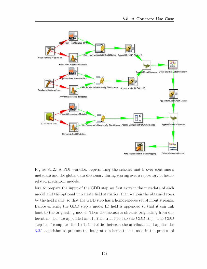
8.5 A Concrete Use Case
Figure 8.12: A PDI workflow representing the schema match over consumer’s
metadata and the global data dictionary during scoring over a repository of heart-
related prediction models.
fore to prepare the input of the GDD step we first extract the metadata of each
model and the optional univariate field statistics, then we join the obtained rows
by the field name, so that the GDD step has a homogeneous set of input streams.
Before entering the GDD step a model ID field is appended so that it can link
back to the originating model. Then the metadata streams originating from dif-
ferent models are appended and further transfered to the GDD step. The GDD
step itself computes the 1 : 1 similarities between the attributes and applies the
3.2.1 algorithm to produce the integrated schema that is used in the process of
147

8.5 A Concrete Use Case
schema matching during scoring. The integrated schema contains an association
between virtual GDD fields and the original fields in the models. To each such
association an marker field is added, indicating that it originates from DeVisa, so
that the ”DeVisa Schema Matcher” step distinguishes it from the metadata rows
originating from the consumer.
On the other side, metadata is extracted and univariate field statistics are
calculated from the consumer’s data stream. The rows are joined based on field
names and some dummy fields are appended to achieve compatibility with the
metadata stream originating from DeVisa GDD. The streams are appended to
each other and the schema matcher step creates all possible valid associations
between consumer’s fields and the original model fields by applying the algorithm
proposed in 5.5.
The analysis of this scenario concludes that enabling integration facilities
within the scoring process provides the premises of easing the KDD processes for
the consumer and potentially getting better results than performing a standard
KDD process. Exploiting mining models based on heterogeneous data sources
can lead to discovering correlations between apparently independent facts that
can lead to further discoveries in the domain.
In the future the data set will be further enriched with new data instances
as well as new attributes and dependencies between attributes materialized in
predictive and statistical models, so that more complex use case can be obtained.
148
Chapter 9
Conclusions and Further Work
In this thesis the conceptual architecture, the functionality and the formal model
of an online scoring system (DeVisa) was presented. The system has been de-
signed to provide unified access to different prediction models using standards
like PMML and web services. From a theoretical perspective, the thesis uses
formalisms from relational model to capture both the structural (statical) and
the behavioral (dynamic) aspects of the system. The original contributions and
future research directions are presented hereunder.
9.1 The Contributions of this Work
Chapter 3 introduces the architecture of a online scoring system called DeVisa in
the context of knowledge as a service paradigm. The system has been designed to
provide uniform and transparent access to heterogeneous prediction models using
standard technologies like PMML and web services. The system assists domain
experts in sharing their predictive capabilities based on their observations without
disclosing the data itself. Besides basic functions such as uploading/downloading
models (administration), the system provides functions such as scoring (a mean to
provide knowledge capabilities) , model comparison, model composition, search-
ing on the stored models through a message style web service interface.
The chapter describes the components of the system (the service layers, the
PMML repository, the metadata catalog, the PMQL library, the PMQL engine)
and the interaction between the components. The predictive models in DeVisa
149

9.1 The Contributions of this Work
are provided by different producer applications, therefore the data dictionaries are
potentially heterogeneous. One of the main components of DeVisa is the meta-
data catalog, which includes a component called global data dictionary, which
behaves live a mediator between heterogeneous data dictionaries in the reposi-
tories. The section 3.2 proposes a technique of updating the global dictionary
as new models are added to the repository (algorithm 3.2.1). The technique is
based on re-calculating a similarity measure between the existing entities and the
new ones, merging attributes if considered identical and maintaining a similarity
matrix that is further used in the online request processing.
To achieve a clear separation between the consumer’s goal and the effective
DeVisa services a specialized language (PMQL) is introduced. It is a XML-based
language used to express communication both with the consumer applications
(requests, answers) and between the internal DeVisa components. The section
3.3.1 describes the structure of a PMQL consumer request. The formal PMQL
specification is presented in A.
The chapter emphasizes the main phases in which a PMQL scoring request is
processed in DeVisa. The consumer sends a goal expressed in PMQL, containing
the data to be scored and specifies a predictive model (exactly or laxly). The
PMQL engine processes the request and uses a library of XQuery functions to
effectively access the repository. The answer is expressed in PMQL as well. In
the scoring process if a model satisfying the request is not found, then the engine
may attempt to infer a new one (composition).
In section 3.4.3 an overview of the model composition problem is provided
and the circumstances in which this problem is reflected in DeVisa.
The chapter 4 provides the theoretical foundation of the system that captures
two different perspectives: structural and behavioral. The structural perspective
focuses on the main entities that DeVisa is composed of: the data dictionaries,
mining schemas, the metadata catalog, the model repository. The section 4.1.1
introduces the concept of mining functional dependency and the property 4.1
proves that it is stronger than the functional dependency in relational model. In
consequence, the Armstrong’s set of axioms is sound and complete for MFDs.
This result enables the definition of a formal framework in which new models can
be derived from the ones in the DeVisa repository.
150

9.1 The Contributions of this Work
Besides the structural perspective the chapter provides a behavioral perspec-
tive, that includes the scoring process and the model composition process. The
scoring process described in 4.2 is split into the component phases depending on
the consumer’s request type and a formal model of each of the phases is provided.
The first phase, called model discovery, is the most complex in the match schema
case, in which the consumer has the possibility to describe its own schema that
might not conform exactly to the ones in DeVisa repository (4.2.1.2). The prop-
erty 4.2 proves that in order to find the models that are best applicable on a data
set, we need to find the optimal derivable match function, which will be described
further in 5.5.
In section 4.3 a theoretical foundation on the data mining models composition
problem within DeVisa was presented. The work identifies the contexts in which
model composition can occur (either implicit, during scoring or explicit, specified
in the consumer’s goal) and analyzes the possible approaches. The formal infer-
ence framework based on the MFD concept introduced in 4.1.1 is used to achieve
model composition in DeVisa. The section 4.3.1.2 that in the scoring process or
implicit composition the derivability of a mining model from a data dictionary is
similar with the notion of consequence of a functional dependency from a set of
functional dependencies, and, therefore, similar techniques can be used for this
decision problem in DeVisa.
The chapter 5 introduces a new 1:1 schema matching technique and a hybrid
adaptive similarity function, both designed to be applied on mining schemas
expressed in PMML.
The schema matching technique is customized to take advantage of the in-
ternal DeVisa configuration. It uses the global data dictionary as the front row
mediated schema that filters out unfeasible match candidates and at the end
produces a local matching between the consumer’s schema and the data dictio-
naries in DeVisa (5.5.1). To match the remaining attributes, a flow network
modeling is used (5.5.2), but adapted to integrate additional constraints that are
specific to the DeVisa configuration, such as validity and derivability. Further-
more the technique exploits the obtained network topology to further improve
the efficiency of the matching technique (5.5.5, 5.5.6, 5.5.7). While applying the
matching algorithm an optimal match needs to be calculated, the one with the
151

9.1 The Contributions of this Work
maximum support and confidence (5.5.3). However, the derivability restriction
prevails to the optimality and therefore sub-optimal solutions are accepted pro-
vided that they satisfy the restriction. Some useful properties related to the
underlying graph topology are stated and proven (such as 5.4, 5.5, 5.7,5.8). The
thesis proves the correctness of the provided schema matching algorithm (prop-
erty 5.5.3) and that the matching algorithm correctly solves the model discovery
problem in polynomial time (property 5.10).
The similarity measure proposed in section 5.6 is calculated by aggregating
several similarity criterions, such as short name, display name, data type, textual
description, semantic sense, statistic information, structural information (tax-
onomies, ontologies) and data instances, using an adaptive technique that takes
into consideration only the information available at runtime.
The chapter 7 presents the current status of implementation of the system:
the PMQL specication, the metadata catalog specification, the schema matching
technique implementation, similarity function the PMQL and admin web service,
the XQuery scoring functions, the XQuery library, Weka PMML export.
The chapter 8 investigates the potential applications of the system in differ-
ent contexts and application domains. It mainly can be integrated as a decision
support module in a SOA. Application domains as e-Health systems, multi-agent
interface agents systems, credit risk assessment, or bioinformatics applications are
some usage examples. A concrete use case was presented using the heart-disease,
arrhythmia and echocardiogram databases from the UCI machine learning repos-
itory, in which the DeVisa functionality is incorporated in a data integration
visual tool (PDI) in which the scoring process is modeled through the use of data
flows. In the section 8.5.3 a ROC analysis is provided for an implicit late compo-
sition use case based on the heart disease database, showing that incorporating
integration facilities in the scoring process can lead to improved prediction capa-
bilities with performance higher than the average performance of the individual
predictions.
152

9.2 Further Research Dirrections
9.2 Further Research Dirrections
The research performed during this work has opened a suite of open research
paths that can further enrich the DeVisa system. These directions are presented
hereunder.
First of all, the current work has focused merely on classification. Although
PMML and therefore DeVisa can store other type of predictive models, no formal
way of dealing with those has been provided. An open direction is investigating
the DeVisa behavioral aspects related to the clustering models.
The work introduced a formal framework for determining the derivability of a
mining schema in a data dictionary using the concept of mining functional depen-
dency. Further work will investigate the implications of other type of relational
restrictions, such as multi-valuate dependencies or inclusion dependencies.
In the scoring process, if several match functions are found and no other
constraint / recommendation is found, the system returns several answers to the
consumer. The consumer needs to perform a manual validation process to choose
the right mapping. If a feedback would be given back to DeVisa, it should be
able to store a schema alignment (match functions, according to the terminology
used in 5.5) for future use. Future work will include a match feedback mechanism
and will update the schema matching algorithm to consult the stored alignments.
At this moment the similarity measure assigns equal weights to the available
match criteria. In the future the technique is going to be refined so that employs
probabilistic rule sets to adapt the weighting scheme to achieve better accuracy.
Also the matching technique will be refined to seamlessly incorporate the addi-
tional constraints. Another research direction is improving the schema matching
strategy to allow n : 1 mappings.
The future work will include the investigation of a clustering technique for cre-
ating and maintaining the GDD, i.e it will behave like a partition matrix, in which
entities are mapped to clusters with a certain degree of confidence. The schema
matching technique will be likely to take advantage of such a representation.
The freshness of a model is one of the factors where the accuracy of a model
strongly depends on. In the current implementation the freshness of a model
is a feature that depends only on a model producer. DeVisa cannot control
153
9.2 Further Research Dirrections
that aspect, so models can get outdated very easily. However the consumer can
specify the freshness and DeVisa can rank the models from that point of view.
One possible solution is that DeVisa will trigger the upload of the models using
web service interfaces of model producers.
In the DeVisa system the collection of models together with the related on-
tologies form a knowledge base, which aims to be integrated in the context of
Semantic Web applications.. A good research direction is designing a technique
of ensuring consistency of the knowledge base. Each upload triggers a check-up
against the existing knowledge base and a conflict might occur. There are a few
ways of dealing with conflicts: reject the whole knowledge base (FOL approach,
but unacceptable under the web setup), determine the maximal consistent subset
of the knowledge base, or use a para-consistent logic approach. The knowledge
base facilitates that new knowledge is derived from it, so that DeVisa can include
in the future rule management and inference engines (RuleML).
Another item which is part of the DeVisa roadmap is extending the PDI tool
to incorporate most of the DeVisa functionality so that interoperability and shar-
ing of prediction capability can be manipulated by end users. One of the main
benefits of incorporating Devisa functions in such a front end is the broad acces-
sibility of the knowledge resulted from the application of prediction models. The
front end can be shifted to a web setup, that can lead to evolution of user com-
munities interested in modeling the same domain and provides the premises that
the prediction models are refined and improved through the action of collective
expertise.
154
Appendix A
PMQL Specification
<xs:schema targetNamespace="http://www.infoiasi.ro/dgorea/devisa/pmql"
elementFormDefault="unqualified"
xmlns:xs="http://www.w3.org/2001/XMLSchema"
xmlns="http://www.infoiasi.ro/dgorea/devisa/pmql"
xmlns:dm="http://www.dmg.org/PMML-3_2">
<xs:import namespace="http://www.dmg.org/PMML-3_2"
schemaLocation="http://www.dmg.org/v3-2/pmml-3-2.xsd"/>
<xs:complexType name="DataType">
<xs:sequence>
<xs:element name="instance" minOccurs="1" maxOccurs="unbounded">
<xs:complexType>
<xs:sequence>
<xs:element name="field" minOccurs="1"
155

maxOccurs="unbounded">
<xs:annotation/>
<xs:complexType>
<xs:attribute name="name" type="xs:string"/>
<xs:attribute name="value" type="xs:string"/>
</xs:complexType>
</xs:element>
</xs:sequence>
</xs:complexType>
</xs:element>
</xs:sequence>
</xs:complexType>
<xs:complexType name="ModelSpecType">
<xs:choice minOccurs="1" maxOccurs="1">
<xs:element name="Model">
<xs:annotation>
<xs:documentation>
A reference to an existing DeVisa Model
</xs:documentation>
</xs:annotation>
<xs:complexType>
<xs:attribute name="ref" type="xs:string" use="required"/>
</xs:complexType>
</xs:element>
156

<xs:element name="MiningSchemaRef">
<xs:annotation>
<xs:documentation>
A reference to an existing DeVisa Mining Schema
</xs:documentation>
</xs:annotation>
<xs:complexType>
<xs:attribute name="ref" type="xs:string"/>
</xs:complexType>
</xs:element>
<xs:sequence>
<xs:annotation>
<xs:documentation>Exact Data Dictionary Specification:
A list of DeVisa data dictionaries where the schema is
going to be looked up is provided.
</xs:documentation>
</xs:annotation>
<xs:element name="DataDictionaryRef"
minOccurs="0" maxOccurs="unbounded">
<xs:complexType>
<xs:attribute name="ref" type="xs:string"/>
</xs:complexType>
</xs:element>
<xs:element ref="dm:MiningSchema"/>
157

</xs:sequence>
<xs:sequence>
<xs:annotation>
<xs:documentation>Lax Schema Specification: A data dictionary
and a mining schema is described. The engine needs to look for
a matching data dictionary and, whithin the data dictionary, for
corresponding matching mining schema</xs:documentation>
</xs:annotation>
<xs:element ref="dm:DataDictionary"/>
<xs:element ref="dm:MiningSchema"/>
</xs:sequence>
</xs:choice>
<xs:attribute name="version">
<xs:simpleType>
<xs:restriction base="xs:string">
<xs:pattern value="\d+\.\d*"/>
</xs:restriction>
</xs:simpleType>
</xs:attribute>
<xs:attribute name="task">
<xs:simpleType>
<xs:restriction base="xs:string">
<xs:enumeration value="classification"/>
158

<xs:enumeration value="clustering"/>
<xs:enumeration value="rules"/>
</xs:restriction>
</xs:simpleType>
</xs:attribute>
</xs:complexType>
<xs:complexType name="RequestType">
<xs:choice>
<xs:element name="score" type="ScoreRequestType"/>
<xs:element name="search" type="SearchRequestType"/>
<xs:element name="compare" type="CompareRequestType"/>
<xs:element name="compose" type="ComposeRequestType"/>
<xs:element name="statistics" type="xs:anySimpleType"/>
</xs:choice>
</xs:complexType>
<xs:complexType name="ScoreRequestType">
<xs:sequence>
<xs:element ref="modelSpec" minOccurs="1"
maxOccurs="unbounded"/>
<xs:element ref="data" minOccurs="1" maxOccurs="1"/>
</xs:sequence>
<xs:attribute name="function" type="xs:string"/>
</xs:complexType>
159
<xs:complexType name="SearchRequestType">
<xs:sequence>
<xs:element ref="modelSpec"/>
</xs:sequence>
</xs:complexType>
<xs:complexType name="CompareRequestType">
<xs:sequence>
<xs:element ref="modelSpec" minOccurs="2" maxOccurs="2"/>
</xs:sequence>
<xs:attribute name="type" use="required">
<xs:simpleType>
<xs:restriction base="xs:string">
<xs:enumeration value="syntactic"/>
<xs:enumeration value="semantic"/>
</xs:restriction>
</xs:simpleType>
</xs:attribute>
</xs:complexType>
<xs:complexType name="ComposeRequestType">
<xs:sequence>
<xs:element ref="modelSpec" maxOccurs="1" minOccurs="1"/>
<xs:element ref="data" maxOccurs="1" minOccurs="0"/>
</xs:sequence>
<xs:attribute name="type" use="required">
<xs:simpleType>
160

<xs:restriction base="xs:string">
<xs:enumeration value="selection"/>
<xs:enumeration value="sequencing"/>
<xs:enumeration value="stacking"/>
</xs:restriction>
</xs:simpleType>
</xs:attribute>
</xs:complexType>
<xs:complexType name="AnswerType">
<xs:choice>
<xs:element name="score" type="ScoreAnswerType"/>
<xs:element name="search" type="SearchRequestType"/>
<xs:element name="compare" type="CompareRequestType"/>
<xs:element name="compose" type="ComposeRequestType"/>
<xs:element name="statistics" type="xs:anySimpleType"/>
</xs:choice>
</xs:complexType>
<xs:complexType name="ScoreAnswerType">
<xs:sequence>
<xs:element ref="data"/>
</xs:sequence>
</xs:complexType>
<xs:complexType name="CompareAnswerType">
<xs:choice>
161

<xs:element name="sintactic">
<xs:complexType>
<xs:attribute name="identical" type="xs:boolean"/>
</xs:complexType>
</xs:element>
<xs:element name="semantic">
<xs:complexType> <xs:sequence>
<xs:element name="schemaCompatible" type="xs:boolean"/>
<xs:element name="functionCompatible">
<xs:complexType><xs:sequence>
<xs:element name="function">
<xs:simpleType>
<xs:restriction base="xs:string">
<xs:enumeration value="identical"/>
<xs:enumeration value="different"/>
</xs:restriction>
</xs:simpleType>
</xs:element>
<xs:element name="algorithm">
<xs:simpleType>
<xs:restriction base="xs:string">
<xs:enumeration value="identical"/>
<xs:enumeration value="different"/>
</xs:restriction>
</xs:simpleType>
162

</xs:element>
</xs:sequence> </xs:complexType>
</xs:element>
</xs:sequence> </xs:complexType>
</xs:element>
</xs:choice>
</xs:complexType>
<xs:element name="modelSpec" type="ModelSpecType"/>
<xs:element name="data" type="DataType"/>
<xs:element name="request" type="RequestType"/>
<xs:element name="answer" type="AnswerType"/>
<xs:element name="pmql" type="PmqlType"/>
<xs:complexType name="PmqlType">
<xs:choice>
<xs:element ref="request"/>
<xs:element ref="answer"/>
</xs:choice>
</xs:complexType>
</xs:schema>
163

Appendix B
Catalog Schema
<?xml version="1.0" encoding="UTF-8"?>
<schema targetNamespace="http://www.infoiasi.ro/~dgorea/devisa/metadata"
elementFormDefault="qualified" xmlns="http://www.w3.org/2001/XMLSchema"
xmlns:dm="http://www.infoiasi.ro/~dgorea/devisa/metadata">
<include schemaLocation="types.xsd"/>
<element name="catalog">
<complexType>
<sequence>
<element ref="dm:collections" minOccurs="1"
maxOccurs="1"/>
<element ref="dm:producers" minOccurs="1" maxOccurs="1"/>
<element ref="dm:DataDictionaries" minOccurs="1" maxOccurs="1"/>
<element ref="dm:models" minOccurs="1" maxOccurs="1"/>
</sequence>
</complexType>
164

</element>
<element name="collection">
<complexType>
<sequence>
<element name="description" type="string"/>
</sequence>
<attribute name="id" type="ID" use="required"/>
<attribute name="uri" type="anyURI" use="optional"/>
<attribute name="localName" type="string" use="required"/>
</complexType>
</element>
<element name="collections">
<complexType>
<sequence>
<element ref="dm:collection" maxOccurs="unbounded"
minOccurs="1"/>
</sequence>
</complexType>
</element>
<element name="modelRef">
<complexType>
<sequence>
<element name="description" type="string" minOccurs="0"
maxOccurs="1" />
<element ref="dm:modelStats" minOccurs="0"
165
maxOccurs="1" />
<element name="MiningSchema" type="dm:MiningSchemaType"
minOccurs="0" maxOccurs="1" />
</sequence>
<attribute name="name" type="string"/>
<attribute name="function" type="IDREF" use="required"/>
<attribute name="algorithmType" type="IDREF" use="required"/>
<attribute name="uri" type="anyURI"/>
<attribute name="collection" type="IDREF"/>
<attribute name="dataDictionary" type="IDREF"/>
</complexType>
</element>
<element name="modelStats">
<complexType>
<sequence>
<element name="instancesNumber" type="int"/>
</sequence>
</complexType>
</element>
<element name="dataDictionaries">
<complexType>
<sequence>
<element ref="dm:dataDictionaryRef"/>
</sequence>
</complexType>
166
</element>
<element name="dataDictionaryRef">
<complexType>
<attribute name="idref" type="IDREF"/>
<attribute name="uri" type="anyURI"/>
<attribute name="localName" type="string"/>
</complexType>
</element>
<element name="models" >
<complexType>
<sequence>
<element ref="dm:modelRef" minOccurs="0" maxOccurs="unbounded">
</element>
</sequence>
</complexType>
</element>
<element name="producers">
<complexType>
<sequence>
<element ref="dm:producer" minOccurs="0"
maxOccurs="unbounded"/>
</sequence>
</complexType>
</element>
<element name="producer" >
167
<complexType>
<attribute name="id" type="ID"/>
<attribute name="uri" type="anyURI"/>
<attribute name="localName" type="string"/>
</complexType>
</element>
<element name="functions">
<complexType>
<sequence>
<element ref="dm:function"/>
</sequence>
</complexType>
</element>
<element name="function">
<complexType>
<sequence>
<element ref="dm:algorithm" minOccurs="1" maxOccurs="unbounded"/>
</sequence>
<attribute name="id" type="ID"/>
<attribute name="uri" type="anyURI"/>
<attribute name="localName" type="string"/>
</complexType>
</element>
<element name="algorithm">
<complexType>
168

<sequence>
<element ref="dm:algorithmType" minOccurs="1" maxOccurs="unbounded"/>
</sequence>
<attribute name="id" type="ID"/>
<attribute name="uri" type="anyURI"/>
<attribute name="localName" type="string"/>
</complexType>
</element>
<element name="algorithmType">
<complexType>
<attribute name="id" type="ID"/>
<attribute name="uri" type="anyURI"/>
<attribute name="localName" type="string"/>
</complexType>
</element>
</schema>
169

Appendix C
Use Cases
Figure C.1: The scoring use case.
170

Figure C.2: The explicit model composition use case.
171


Figure C.4: The object model of the PMQL engine component in DeVisa.
173

Appendix D
List of Acronyms
CAD Coronary Artery Disease
CRISP-DM Cross Industry Standard
for Data Mining
DD Data Dictionary
DM Data Mining
DOM Document Object Model
ER Entity Relationship
ESB Enterprise Service Bus
FOL First Order Logic
GDD Global Data Dictionary
IML Inductive Machine Learning
JDM Java Data Mining
KDD Knowledge Discovery in Databases
MFD Mining Functional Dependency
MS Mining Schema
PCDATA Parsed Character Data
PDI Pentaho Data Integration
PMML Predictive Model Markup Lan-
guage
PMQL Predictive Model Query Language
SAX Simple API for XML
SOA Service Oriented Architecture
SOAP Simple Object Access Protocol
SVM Support Vector Machine
REST Representational State Transfer
UCI Universiy of California - Irvine
XML Extensible Markup Language
XMLA XML for Analysis
XMLDB XML Database
XML-RPC XML Remote Procedure Call
XSL XML Stylesheet
XSLT XSL Transformation
174
References
*** (2003a). XML-RPC home page. http://www.xmlrpc.com/. 32, 124
*** (2003b). XML:DB initiative for XML databases.
http://xmldb-org.sourceforge.net/. 124
*** (2004a). Sax home page. http://www.saxproject.org/. 123
*** (2004b). The WS-resource framework. http://www.globus.org/wsrf/. 118
*** (2005). JSR 73: Data Mining API. http://jcp.org/en/jsr/detail?id=73.
22, 26, 119, 120
(2006). Wordnet - a lexical database for the english language.
http://wordnet.princeton.edu/. 78
*** (2007a). JSR 173: Streaming API for XML.
http://jcp.org/en/jsr/detail?id=173. 123
*** (2007b). Soap version 1.2 part 1: Messaging framework (second edition).
http://www.w3.org/TR/soap12-part1/. 31, 40, 124
(2007). Web ontology language (owl). http://www.w3.org/2004/OWL/. 85
*** (2007c). Weka4ws: distributed data mining using web services.
http://grid.deis.unical.it/weka4ws/. 118
(2007). XML path language (XPath) 2.0. http://www.w3.org/TR/xpath20/. 124
(2007). Xquery 1.0 and xpath 2.0 data model (xdm).
http://www.w3.org/TR/xpath-datamodel/. 123, 124
175

REFERENCES
(2008). Amazon simple storage service (amazon s3).
http://www.amazon.com/s3. 117, 120
(2008). Apache axis2. http://ws.apache.org/axis2/index.html. 125
*** (2008a). Pentaho data integration. 137
*** (2008b). The R project for statistical computing.
http://www.r-project.org. 119
*** (2008c). Sourceforge.net Open Source Software. http://sourceforge.net.
126
*** (2008d). XML for Analysis. 22
(2008). XML schema part 2: Datatypes second edition.
http://www.w3.org/TR/xmlschema-2/. 24
Aberer, K. (2003). Special topic section on peer to peer data management. 77
Agrawal, R. & ad A. Swami, T.I. (1993). Mining association rules between
sets of items in large databases. In Proceedings of the 1993 ACM-SIGMOD
International Conference on Management of Data, 207–216. 12
Agrawal, R. & Srikant, R. (1994). Fast algorithm for mining association
rules. In Proceedings of the 1994 International Conference on Very Large
Databases (VLDB), Santiago, Chile, 487–499. 13
Alboaie, L., Gorea, D. & Felea, V. (2008a). Semantic integrity control
in the database layer of an e-health system. In International Journal of Com-
puters, Communications and Control (IJCCC), Proceedings of the IEEE 2nd
International Conference on Computers, Communications and Control , vol.
III. 129
Alboaie, L., Gorea, D. & Felea, V. (2008b). A SSO-style authentication
in a SOA-based e-health system. In I.T. M. Simion, ed., Proceedins of the 32nd
Annual Conference of the American Romanian Academy of Arts and Sciences
2008, Boston, Wentworth Institute of Technology, Boston MA, USA. 130
176

REFERENCES
Ali, A., Rana, O. & Taylor, I. (2005). Web services composition for dis-
tributed data mining. In Parallel Processing, 2005. ICPP 2005 Workshops.
International Conference Workshops on, 11 –18, IEEE Computer Society. 2,
118
Armstrong, W. (1974). Dependency structures of data base relationships. In
N.H.P. Co., ed., Proceedings of IFIP74 , 580–583. 57
Asuncion, A. & Newman, D. (2007). UCI machine learning repository. 134
Aumueller, D., Do, H.H., Massmann, S. & Rahm, E. (2005). Schema and
ontology matching with COMA++. In SIGMOD ’05: Proceedings of the 2005
ACM SIGMOD international conference on Management of data, 906–908,
ACM, New York, NY, USA. 85
Axis (2007). Apache axis. http://ws.apache.org/axis/. 31
Bargiela, A. & Pedrycz, W. (2003). Granular Computing: An Introduction.
Kluwer Academic Publishers. 20
Bellman, R. (1958). On a routing problem. Quarterly of Applied Mathematics,
16, 87–90. 103
Bergamaschi, S., Castano, S., Vincini, M. & Beneventano, D. (2001).
Semantic integration of heterogeneous data sources. Data and Knowledge En-
gineering , 36, 215–249. 83
Berners-Lee, T. (2006). Notation 3: A readable RDF syntax.
http://www.w3.org/DesignIssues/Notation3. 21
Bernstein, P.A. & Rahm, E. (2000). Data warehouse scenarios for model
management. In In International Conference on Conceptual Modeling , 1–15,
Springer. 76
Biggs, D., de Ville, B. & Suen, E. (1991). A method of choosing multiway
partitions for classification and decision trees’. 18, 49–62. 15
177

REFERENCES
Breiman, L. (1984). Classification and regression trees. Belmont, Wadsworth.
15
Breiman, L. (1996). Bagging predictors. In Machine Learning , 123–140. 47
Castano, S. & Antonellis, V. (1999). A schema analysis and reconciliation
tool environment. In Proceedings of of the International Database Engineering
and Applications Symposium. 82
Chang, C. (1976). DEDUCE-a deductive query language for relational data
bases. Acknowledgments Pattern Recognition and Artifical Intelligence, 108. 71
Chang, C. & Lee, R. (1973). Symbolic logic and mechanical theorem proving.
Academic Press New York and London. 72
Chaves, J., Curry, C., Grossman, R.L., Locke, D. & Vejcik, S. (2006).
Augustus: the design and architecture of a PMML-based scoring engine. In
DMSSP ’06: Proceedings of the 4th international workshop on Data mining
standards, services and platforms, 38 – 46, ACM, New York, NY, USA. 119
Chieh-Yuan Tsai, M.H.T. (2005). A dynamic web service based data min-
ing process system. In The Fifth International Conference on Computer and
Information Technology CIT 2005 , 1033– 1039. 117
Cios, K. & Kurgan, L. (2005). Trends in data mining and knowledge discovery.
Advanced Techniques in Knowledge Discovery and Data Mining , 1–26. viii, 1,
7, 10, 11
Cios, K., Pedrycz, W., Swiniarski, R. & Kurgan, L. (2007). Data Mining.
A Knowledge Discovery Approach. Springer. 17, 22
Clarke, J. & Seo, D. (2008). An ensemble approach to improved prediction
from multitype data. Pushing the Limits of Contemporary Statistics: Contri-
butions in Honor of Jayanta K. Ghosh, 3, 302–317. 136
Cohen, W., Ravikumar, P. & Fienberg, S. (2003). A comparison of string
metrics for matching names and records. In Proceedings of the KDD-2003
Workshop on Data Cleaning and Ob ject Consolidation. 109
178
REFERENCES
Cohen, W.W. & Singer, Y. (1999). A simple, fast, and effective rule learner.
In In Proceedings of the Sixteenth National Conference on Artificial Intelli-
gence, 335–342, AAAI Press. 16
Crawford, S. (1989). Extensions to the CART algorithm. International Journal
of Man-Machine Studies, 31, 197–217. 16
Curino, C., Orsi, G. & Tanca, L. (2007). X-SOM: A flexible ontology map-
per. In DEXA Workshops , 424–428, IEEE Computer Society. 85
Davies, J., Studer, R. & Warren, P. (2006). Semantic Web Technologies
Trends and Research in Ontology-based Systems. John Wiley and Sons, West
Sussex, England. 73, 81
de Bruijn, J., Ehrig, M., Feier, C., n Recuerda, F.M., Scharffe, F. &
Weiten, M. (2006). Ontology Mediation, Merging, and Aligning . John Wiley
and Sons. 75
Dean, J. & Ghemawat, S. (2008). MapReduce: Simplified data processing on
large clusters. Communications of the ACM , 51, 107–113. 117
Detrano, R., Janosi, A., Steinbrunn, W., Pfisterer, M., Schmid, J.,
Sandhu, S., Guppy, K., Lee, S. & Froelicher, V. (1989). International
application of a new probability algorithm for the diagnosis of coronary artery
disease. American Journal of Cardiology , 64, 304—310. 135
DeVisa (2007). DeVisa. http://devisa.sourceforge.net. 2, 39, 40
Dhamankar, R., Lee, Y., Doan, A., Halevy, A. & Domingos, P. (2004).
imap: Discovering complex semantic matches between database schemas. In
Proceedings of the ACM SIGMOD international conference on Management of
data, June 13-18, 2004, Paris, France, 383–394. 84
DMG (2008). Data mining group. http://www.dmg.org. 2, 22, 120
Doan, A. & Halevy, A.Y. (2005). Semantic integration research in the
database community: A brief survey. AAAI Magazine, 26, 83–94. 76, 81
179

REFERENCES
Doan, A., Domingos, P. & Halevy, A. (2001). Reconciling schemas of dis-
parate data sources: A machine-learning approach. In Proceedings of the SIG-
MOD Conference, 509–520. 83
Doan, A., Madhavan, J., Domingos, P. & Halevy, A. (2004). Ontology
matching: A machine learning approach. In Handbook on Ontologies in Infor-
mation Systems , 397–416, Springer. 85
Dowling, W. & Gallier, J. (1984). Linear time algorithms for testing the
satisfiability of propositional Horn formulae. Journal of Logic Programming , 3,
276–284. 70
Dunn, H.L. (1946). Record linkage. American Journal of Public Health, 36,
1412–1416. 77
Edmonds, J. (2008). How to think about Algorithms, chap. Network Flows and
Linear Programming. 15, Cambridge University Press. 94
Edmonds, J. & Karp, R.M. (1972). Theoretical improvements in algorithmic
efficiency for network flow problems. Journal of the ACM , 19, 248–264. 94
Edwards, D. (1995). Introduction to Graphical Modeling . Springer-Verlag. 21
Erl, T. (2005). Service-oriented Architecture: Concepts, Technology, and De-
sign. Prentice Hall. 125
eXist (2007). Exist - open source native xml database.
http://www.exist-db.org/. 34, 124
Fagin, R. (1977). Functional dependencies in a relational data base and propo-
sitional logic. IBM Journal of Research and Development , 21, 543–544. 70,
72
Fasulo, D. (1999). An analysis of recent work on clustering algorithms. Techni-
cal Report 01-03-02, University of Washington. 7
180
REFERENCES
Fayyad, U., Piatetsky-Shapiro, G. & Smyth, G. (1996a). The KDD pro-
cess for extracting useful knowledge from volumes of data. Communications of
the ACM , 39, 27–34. 1, 8
Fayyad, U.M., Piatetsky-Shapiro, G. & Smyth, P. (1996b). From Data
Mining to Knowledge Discovery: An Overview., vol. Advances in Knowledge
Discovery and Data Mining, chap. 1, 1–34. AAAI Press/ The MIT Press. 6
Felea, V. (1996). Baze de date relationale. Dependente.. Editura Universitatii
Al. I. Cuza Iasi. 71
Fensel, D., Lausen, H., Polleres, A., de Bruijn, J., Stollberg, M.,
Roman, D. & Domingue, J. (2007). Enabling Semantic Web Services.
Springer, Berlin Heidelberg. 77
Ferrucci, D., Grossman, R.L. & Levas, A. (2006). PMML and UIMA based
frameworks for deploying analytic applications nd services. In Proceedings of the
4th International Workshop on Data Mining Standards, Services and Platforms
(DM-SSP 06), 14–26, ACM, New York. 118
Fielding, R.T. (2000). Architectural Styles and the Design of Network-based
Software Architectures. Ph.D. thesis, University of California. 32
Fisher, D. (1996). Iterative optimization and simplification of hierarchical clus-
terings. Journal of Artificial Intelligence Research, 4, 147–178. 16
Ford, L.R. & Fulkerson, D.R. (1956). Maximal flow through a network.
Canadian Journal of Mathematics, 8, 399 – 404. 93
Ford, L.R. & Fulkerson, D.R. (1962). Flows in networks. Princeton Uni-
versity Press. 93
Freund, Y. & E.Schapire, R. (1997). A decision-theoretic generalization of
on-line learning and an application to boosting. Journal of Computer and Sys-
tem Sciences . 47
181
REFERENCES
Garcia-Molina, H., Papakonstantinou, Y., Quass, D., Rajaraman,
A., Sagiv, Y., Ullman, J. & Widom, J. (1997). The TSIMMIS project:
Integration of heterogeneous information systems. Journal of Intelligent Infor-
mation Systems , 8. 76
Geist, I. & Sattler, K. (2002). Towards data mining operators in database
systems: Algebra and implementation. In Proceedings of the DBFusion Inter-
national Workshop on Databases, Documents, and Information Fusion, vol.
124, CEUR-WS, Karlsruhe, Germany. 18
Gennari, J., Langley, P. & Fisher, D. (1989). Models of incremental con-
cept formation. Artificial Intelligence, 40, 11–61. 135
Ghemawat, S., Gobioff, H. & Leung, S.T. (2003). The Google file system.
In The ACM Symposium on Operating Systems Principles. 117
Giarratano, J. & Riley, G. (1994). Expert Systems: Principles and Pro-
gramming . PWS Publishing, 2nd edn. 20
Giunchiglia, F., Shvaiko, P. & Yatskevich, M. (2004). S-Match: an algo-
rithm and an implementation of semantic matching. In C. Bussler, J. Davies,
D. Fensel & R. Studer, eds., ESWS , vol. 3053 of Lecture Notes in Computer
Science, 61–75, Springer. 84
GO (2007). The gene ontology. http://www.geneontology.org. 132
Gorea, D. (2005a). A comparative analisys between open source XML database
systems. In Linux and Virtual Learnig Environments Symposium. 123
Gorea, D. (2005b). Towards using XML database systems in web-based learn-
ing systems. In Proceedings of the National Conference on Virtual Learning,
Bucharest . 123
Gorea, D. (2005c). A XML based method for learning in interface agents sys-
tems. In ROCHI 2005 Romanian Symposium of Human Computer Interaction,
Cluj, Romania. 3, 131
182
REFERENCES
Gorea, D. (2006a). Towards new tools for e-training within an enterprise in-
tranet. In National Conference on Virtual Learning, Octombrie 28-29, 2006,
Bucharest, Romania. 134
Gorea, D. (2006b). Towards technologies for resource organization and access
in intranet systems. In Proceedings of the Romanian Symposium in Computer
Science, Iasi, Romania. 134
Gorea, D. (2007). Towards storing and interchanging data mining models. In
K. Boyanov, R. Nikolov, I. Nikolova & M. Nisheva, eds., Proceedings of the
3rd Balkan Conference in Informatics, vol. 2, 229–236, State Agency for ITC,
Sofia University, Bulgarian Academy of Sciences, Demetra Ltd. 3, 132
Gorea, D. (2008a). DeVisa. Concepts and Architecture of a Data Mining Models
Scoring and Management Web System. In Proceedings of the 10th International
Conference on Enterprise Information Systems, Barcelona, Spain, INSTICC.
3, 132
Gorea, D. (2008b). Dynamically Integrating Knowledge in Applications. An
Online Scoring Engine Architecture. In Proceedings of the International Con-
ference on Development and Application Systems, 9th Edition, Suceava Roma-
nia. 3
Gorea, D. (2008c). Knowledge as a Service. An Online Scoring Engine Architec-
ture. In Proceedings of The Third International Multi-Conference on Comput-
ing in the Global Information Technology ICCGI 2008, Athens Greece, IEEE
Computer Society Press. 3
Gorea, D. (2008d). Towards online composition of PMML prediction models.
In Proceedings of the 3rd International Conference on Software and Data Tech-
nologies ICSOFT 2008, Porto, Portugal . 3, 51
Gorea, D. & Buraga, S. (2006). Towards integrating decision tree with XML
technologies. In Proceedings of the 8th International Conference on Develop-
ment and Application Systems – DAS 2006, Suceava University Press , Suceava
University Press. 3
183

REFERENCES
Gorea, D. & Felea, V. (2005). A machine learning approach in establishing
reliability of customers in banking applications. In IE2005: International Con-
ference of Information in Economy, Bucuresti, Romania, May 19-20, 2005,,
ISBN 973-8360-014-8, 1161–1167. 3, 132
Gorea, D. & Felea, V. (2006). Towards new collaborative tools for e-training.
In International Scientific Conference ”E-learning and educational Software,
Bucuresti, Romania. 134
Gorea, D. & Moreau, J. (2006). Towards management of enterprise intranet
resources using open source technologies. In Hephaistos Conference, First In-
ternational Conference on Open SourceCollaborative Development Platforms,
Paris, France, November 16-17, 2006 . 134
Griffiths-Jones, S., Grocock, R., van Dongen, S., Bateman, A. & En-
right, A. (2006). miRBase: microRNA sequences, targets and gene nomen-
clature. Nucleic Acids Res., 34, 140 – 144. 132
Grigorios Tsoumakas, I.V. (2007). An interoperable and scalable web-based
system for classifier sharing and fusion. Expert Systems with Applications , 33,
716–724. 117
Grossman, R., Gu, Y., Gupta, C., Hanley, D., Hong, X. & Krish-
naswamy, P. (2004). Open dmix: High performance web services for dis-
tributed data mining. In 7th International Workshop on High Performance
and Distributed Mining, in association with the Fourth International SIAM
Conference on Data Mining . 118
Grossman, R.L. & Gu, Y. (2008). Data mining using high performance clouds:
Experimental studies using sector and sphere. In Proceedings of The 14th ACM
SIGKDD International Conference on Knowledge Discovery and Data Mining
(KDD 2008), ACM. 2, 118
Guvenir, H.A., Acar, B., Demiroz, G. & Cekin, A. (1997). A supervised
machine learning algorithm for arrhythmia analysis”. In Proceedings of the
Computers in Cardiology Conference, Lund, Sweden. 135
184

REFERENCES
Hamacher, H., Leberling, H. & Zimmermann, H. (1978). Sensitivity anal-
ysis in fuzzy linear programming. Fuzzy Sets and Systems , 1, 269–281. 112
Han, K. & Kamber, M. (2001). Data Mining: Concepts and Techniques . Mor-
gan Kaufmann, San Francisco, USA. 20
Hand, D., Mannila, H. & Smyth, P. (2001). Principles of Data Mining . The
MIT Press. 7
Hepp, M., de Leenheer, P., de Moor, A. & Sure, Y., eds. (2008). Ontology
Management Semantic Web, Semantic Web Services, and Business Applica-
tions . SEMANTIC WEB AND BEYOND Computing for Human Experience,
Springer. 73, 108
Herman, I., Swick, R. & Brickley, D. (2008). Resource description frame-
work (RDF). www.w3.org/RDF/. 21
Hors, A.L., Hegaret, P.L., Wood, L., Nicol, G., Robie, J., Champion,
M. & Byrne, S., eds. (2004). Document Object Model (DOM) Level 3 Core
Specification, http://www.w3.org/TR/DOM-Level-3-Core/. 123
Hyafil, L. & Rivest, R. (1976). Constructing optimal binary decision trees is
NP-complete. Information Processing Letters, 5, 15–17. 14
Ian H. Witten, E.F. (2005). Data Mining Practical Machine Learning Tools
and Techniques . Morgan Kaufmann series in data management systems, Else-
vier, 2nd edn. 7, 47
Jaro, M. (1995). Probabilistic linkage of large public health data files. Statistics
in Medicine, 14, 491–498. 77, 109
Kass, G. (1980). An exploratory technique for investigating large quantities of
categorical data. Journal of Applied Statistics, 29, 119–127. 15
Kay, M. (2008). Saxon: The XSLT and XQuery processor. 124
185

REFERENCES
Krishnaswamy, S., Loke, S.W. & Zaslavsky, A. (2001). Knowledge elic-
itation through Web-based data mining services. Lecture Notes in Computer
Science, 2176, 120–?? 117
Kuncheva, L.I. (2004). Classifier ensembles for changing environments. In J.K.
F. Roli & T. Windeatt, eds., Proc. 5th Int. Workshop on Multiple Classifier
Systems , vol. 3077 of LNCS , 1–15, Springer-Verlag. 48
Kurgan, L., Cios, K. & Dick, S. (2006). Highly scalable and robust rule
learner: performance evaluation and comparison. IEEE Transactions on Sys-
tems, Man, and Cybernetics, Part B , 36, 32–53. 16
Landeweerd, G. (1983). Binary tree versus single level tree classification of
while blood cells. Pattern Recognition, 16, 571–577. 15
Lee, T.B., Hendler, J. & Lassila, O. (2001). The semantic web. Scientific
American. 78
Levenstein, I. (1966). Binary codes capable of correcting deletions, insertions
and reversals. Cybernetics and Control Theory . 109
Li, W.S., Clifton, C. & Liu, S.Y. (2000). Database integration using neural
networks: implementation and experiences. Knowledge Information Systems,
2, 73–96. 84, 87
Lim, T.S. & Shih, Y.S. (2000). A comparison of prediction accuracy, com-
plexity, and training time of thirty-three old and new classification algorithms.
Machine Learning , 40, 203–229. 7
L.Madhavan, Bernstein, P. & Rahm, E. (2001). Generic schema matching
with cupid. In Proceedings of the 27th International Conference on Very Large
Databases (VLDB), 48–58. 83
Lovell, B. & Bradley, A. (1996). The multiscale classifier. IEEE Transac-
tions on Pattern Analysis and Machine Intelligence, 18, 124–137. 16
Meier, W. (2002). eXist: An open source native XML database. Springer LNCS
Series, 2593. 124
186
REFERENCES
Melton, J. & Eisenberg, A. (2001). SQL multimedia and application pack-
ages (SQL/MM). In Special Section on Data Mining for Intrusion Detection
and Threat Analysis, vol. 230, ACM. 22
M.Harries, Sammut, C. & Horn, K. (1998). Extracting hidden context.
Machine Learning , 36, 101–126. 48
Miller, G.A. (1995). Wordnet: a lexical database for english. Communications
of the ACM , 38, 39–41. 78
Miller, R., Haas, L. & Hernandez, M. (2000). Schema mapping as
query discovery. In Proceedings of the International Conference on Very Large
Databases (VLDB). 76
Milo, T. & Zohar, S. (1998). Using schema mapping to simplify heterogeneous
data translation. In Proceedings of the International Conference on Very Large
Databases (VLDB). 81
Monge, A. & Elkan, C. (1996). The field-matching problem: algorithm and
applications. In Proceedings of the second international Conference on Knowl-
edge Discovery and Data Mining . 109
Munkres, J. (1957). Algorithms for the assignment and transportation prob-
lems. Journal of the Society of Industrial and Applied Mathematics , 5, 32–38.
95
Murthy, S., Kasif, S. & Salzberg, S. (1994). A system for induction of
oblique decision trees. Journal of Artificial Intelligence Research, 2. 16
Nam, J.W. (2005). Human microRNA prediction through a probabilistic co-
learning model of sequence and structure. Nucleic Acids Research, 33, 3570–
3581. 132
Needleman, S. & Wunsch, C. (1970). A general method applicable to the
search for similarities in the amino acid sequence of two proteins. Molecular
Biology , 444–453. 109
187

REFERENCES
Palopoli, L., Terracina, G. & Ursino, D. (2000). The system DIKE:
towards the semi-automatic synthesis of cooperative information systems and
data warehouses. In Proceedings of the ADBIS-DASFAA Symposium, 108–117.
81
Pawlak, Z. (1991). Rough sets. Theoretical Aspects of Reasoning about Data.
Kluwer Academic Publishers. 20
Pedrycz, W. (1998). Shadowed sets: representing and processing fuzzy sets.
IEEE transactions on Systems, Man and Cybernetics , B, 103–109. 20
Perkowitz, M. & Etzioni, O. (1995). Category translation: Learning to
understand information on the internet. In In Proc. 15th International Joint
Conference on AI , 930–936, Morgan Kaufmann. 84
PMML (2007). PMML version 3.2. http://www.dmg.org/pmml-v3-2.html. 2,
22, 23, 49
PMQL (2008). Predictive Modeling Query Language.
http://devisa.sourceforge.net/pmql.shtml. 39
Popa, H., Pop, D., Negru, V. & Zaharie, D. (2007). AgentDiscover: A
multi-agent system for knowledge discovery from databases. In Ninth Interna-
tional Symposium on Symbolic and Numeric Algorithms for Scientific Comput-
ing . 8
Pottinger, R.A. & Bernstein, P. (2003). Merging models based on given
correspondences. In Proceedings of the International Conference on Very Large
Databases (VLDB)., 826–873. 76
Predoiu, L., Feier, C., Scharffe, F., Bruijn, J.D., Mart±n-
Recuerda, F., Manov, D. & Ehrig., M. (2005). State-of-the-art survey
on ontology aligning and merging. Tech. rep., Institut AIFB, Universitat Karl-
sruhe. 81
Prodromidis, A., Chan, P. & Stolfo, S. (2000). Meta-learning in dis-
tributed data mining systems: Issues and approaches, chap. 3. AAAI/MIT
Press. 48
188

REFERENCES
Quinlan, J. (1986). Induction of decision trees. Machine Learning , 81–106. 15
Quinlan, J. (1993). C4.5: Programs for Machine Learning . Morgan Kaufmann.
15
Rahm, E. & Bernstein, P.A. (2001). A survey of approaches to automatic
schema matching. VLDB Journal , 10, 200–1. viii, 63, 78, 81, 82
Ritchie, W., Legendre, M. & Gautheret, D. (2007). Rna stem-loops: To
be or not to be cleaved by rnase iii. RNA, 13, 457–462. 132
RuleML (2007). Ruleml. http://www.ruleml.org. 154
Ryutaro, I., Hideaki, T. & Shinichi, H. (2001). Rule induction for concept
hierarchy alignment. In Proceedings of the of the 2nd Workshop on Ontology
Learning at the 17th Int. Joint Conf. on AI . 84
Salzberg, S. (1988). Exemplar-based learning: Theory and implementation.
Tr-10-88, Harvard University, Center for Research in Computing Technology,
Aiken Computation Laboratory, 33 Oxford Street; Cambridge, MA 02138. 136
Sedgewick, R. (2003). Algorithms in Java, Part 5: Graph Algorithms, chap.
Network Flow. Addison Wesley, 3rd edn. 100
Sethi, I. & Sarvarayudu, G. (1982). Hierarchical classifier design using mu-
tual information. IEEE Transactions on Pattern Analysis and Machine Intel-
ligence, 4, 441–445. 15
Sewer, A. (2005). Identification of clustered microRNAs using an ab initio pre-
diction method. BMC Bioinformatics . 132
Shepard, R. (1987). Toward a universal law of generalization for psychological
science. Science, 1317–1323. 115
Smith, T. & Waterman, M. (1981). Identification of common molecular sub-
sequences. Journal of Molecular Biology , 146, 195–197. 109
Sperberg-McQueen, C.M. & Thompson, H. (2008). XML Schema.
http://www.w3.org/XML/Schema. 23, 85
189

REFERENCES
Stoilos, G., Stamou, G., & Kollias, S. (2005). A String Metric for Ontology
Alignment , vol. 3729 of LNCS , 624–637. Springer-Verlag. 110, 111
Sun, X.L. & Rose, E. (2003). Automated schema matching techniques: An
exploratory study 133. ACM SIGMOD Record , 28, 113–136. 81
Sung-Kyu, K. (2006). miTarget: microRNA target-gene prediction using a sup-
port vector machine. BMC Bioinformatics 2006 , 7, 411. 132
Sutinen, E. & Tarhio, J. (1995). : On using q-gram locations in approxi-
mate string matching. In ESA ’95: Proceedings of the Third Annual European
Symposium on Algorithms, 327–340, Springer-Verlag. 109
SW (2007). W3C semantic web activity. http://www.w3.org/2001/sw/. 3, 21,
73, 74, 78
Talia, D., Trunfio, P. & Verta, O. (2005). Weka4WS: a WSRF-enabled
weka toolkit for distributed data mining on grids. In Proc. of the 9th Eu-
ropean Conference on Principles and Practice of Knowledge Discovery in
Databases,(PKDD 2005), Porto, Portugal, October 2005 , vol. 3271 of LNAI ,
309–320, Springer-Verlag. 118
Uschold, M. (2000). Creating, integrating, and maintaining local and global on-
tologies. In Proceedings of the First Workshop on Ontology Learning (OL2000)
in conjunction with the 14th European Conference on Artificial Intelligence
(ECAI2000). 74
Utgoff, P., Berkman, N. & Clouse, J. (1997). Decision tree induction
based on efficient tree restructuring. Machine Learning , 29, 5–44. 16
Weka (2007). Weka 3 - data mining software in java.
http://www.cs.waikato.ac.nz/ml/weka. 118
Winkler, W. (1999). The state record linkage and current research problems.
Tech. rep., Statistics of Income Division, Internal Revenue Service Publication.
77, 109, 112
190

REFERENCES
Wirth, R. & Hipp, J. (2000). CRISP-DM: towards a standard process model for
data mining. In Proceedings of the 4th International Conference on the Practical
Applications of Knowledge Discovery and Data Mining , 29–39, Manchester,
UK. 1
Wolpert, D. (1992). Stacked generalization. Neural Networks, 5, 241 – 260. 47
WSDL (2001). Web services description language. http://www.w3.org/TR/wsdl.
31
XML (2003). Extensible markup language (XML). http://www.w3.org/XML/. 1,
124
XQuery (2007). XQuery 1.0: An XML query language.
http://www.w3.org/TR/xquery/. 41, 124
Xu, S. & Zhang, W. (2005). Knowledge as a service and knowledge breaching.
In SCC ’05: Proceedings of the 2005 IEEE International Conference on Services
Computing , 87–94, IEEE Computer Society, Washington, DC, USA. 30
XUpdate (2003). XUpdate - XML update language.
http://xmldb-org.sourceforge.net/xupdate/. 33
Yan, L., Miller, R., Haas, L. & Fagin, R. (2001). Data driven understand-
ing and refinement of schema mappings. In Proceedings of the ACM SIGMOD ,
vol. 30, 485–496. 80
Zadeh, L. (1996). Fuzzy logic = computing with words. IEEE Transactions on
Fuzzy Systems , 4, 103–111. 20
191