is-

nt ofata- min-

files,

urther-ferenttationonalevel-

bas-prim-

Invited Paper at 23rd German Conf. on Artificial Intelligence (KI ’99), Bonn, Germany, 1999.

Knowledge Discovery in Spatial DatabasesMartin Ester, Hans-Peter Kriegel, Jörg Sander

Institute for Computer Science, University of MunichOettingenstr. 67, D-80538 Muenchen, Germany

{ester | kriegel | sander}@dbs.informatik.uni-muenchen.dehttp://www.dbs.informatik.uni-muenchen.de

Abstract. Both, the number and the size of spatial databases, such as geographicor medical databases, are rapidly growing because of the large amount of data ob-tained from satellite images, computer tomography or other scientific equipment.Knowledge discovery in databases (KDD) is the process of discovering valid,novel and potentially useful patterns from large databases. Typical tasks forknowledge discovery in spatial databases include clustering, characterization andtrend detection. The major difference between knowledge discovery in relationaldatabases and in spatial databases is that attributes of the neighbors of some ob-ject of interest may have an influence on the object itself. Therefore, spatialknowledge discovery algorithms heavily depend on the efficient processing ofneighborhood relations since the neighbors of many objects have to be investi-gated in a single run of a typical algorithm. Thus, providing general concepts forneighborhood relations as well as an efficient implementation of these conceptswill allow a tight integeration of spatial knowledge discovery algorithms with aspatial database management system. This will speed-up both, the developmentand the execution of spatial KDD algorithms. For this purpose, we define a smallset of database primitives, and we demonstrate that typical spatial KDD algo-rithms are well supported by the proposed database primitives. By implementingthe database primitives on top of a commercial database management system, weshow the effectiveness and efficiency of our approach, experimentally as well asanalytically. The paper concludes by outlining some interesting issues for futureresearch in the emerging field of knowledge discovery in spatial databases.

1 Introduction

Knowledge discovery in databases (KDD) has been defined as the process of dcovering valid, novel, and potentially useful patterns from data [9]. Spatial DatabaseSystems (SDBS) (see [10] for an overview) are database systems for the managemespatial data. To find implicit regularities, rules or patterns hidden in large spatial dbases, e.g. for geo-marketing, traffic control or environmental studies, spatial dataing algorithms are very important (see [12] for an overview).

Most existing data mining algorithms run on separate and specially prepared but integrating them with a database management system (DBMS) has the following ad-vantages. Redundant storage and potential inconsistencies can be avoided. Fmore, commercial database systems offer various index structures to support diftypes of database queries. This functionality can be used without extra implemeneffort to speed-up the execution of data mining algorithms. Similar to the relatistandard query language SQL, the use of standard primitives will speed-up the dopment of new data mining algorithms and will also make them more portable.

In this paper, we introduce a set of database primitives for mining in spatial dataes. [1] follows a similar approach for mining in relational databases. Our database

itives (section 2) are based on the concept of neighborhood relations. The proposedprimitives are sufficient to express most of the algorithms for spatial data mining fromthe literature (section 3). We present techniques for efficiently supporting these primi-tives by a DBMS (section 4). Section 5 summarizes the contributions and discusses sev-eral issues for future research.

2 Database Primitives for Spatial Data Mining

The major difference between mining in relational databases and mining in spatialdatabases is that attributes of the neighbors of some object of interest may have an in-fluence on the object itself. Therefore, our database primitives (see [7] for a first sketch)are based on the concept of spatial neighborhood relations.

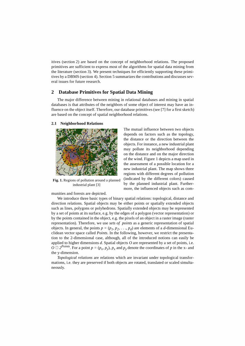
2.1 Neighborhood RelationsThe mutual influence between two objectsdepends on factors such as the topology,the distance or the direction between theobjects. For instance, a new industrial plantmay pollute its neighborhood dependingon the distance and on the major directionof the wind. Figure 1 depicts a map used inthe assessment of a possible location for anew industrial plant. The map shows threeregions with different degrees of pollution(indicated by the different colors) causedby the planned industrial plant. Further-more, the influenced objects such as com-

munities and forests are depicted.We introduce three basic types of binary spatial relations: topological, distance and

direction relations. Spatial objects may be either points or spatially extended objectssuch as lines, polygons or polyhedrons. Spatially extended objects may be representedby a set of points at its surface, e.g. by the edges of a polygon (vector representation) orby the points contained in the object, e.g. the pixels of an object in a raster image (rasterrepresentation). Therefore, we use sets of points as a generic representation of spatialobjects. In general, the points p = (p1, p2, . . ., pd) are elements of a d-dimensional Eu-clidean vector space called Points. In the following, however, we restrict the presenta-tion to the 2-dimensional case, although, all of the introduced notions can easily beapplied to higher dimensions d. Spatial objects O are represented by a set of points, i.e.O ∈ 2Points. For a point p = (px, py), px and py denote the coordinates of p in the x- andthe y-dimension.

Topological relations are relations which are invariant under topological transfor-mations, i.e. they are preserved if both objects are rotated, translated or scaled simulta-neously.

Fig. 1. Regions of pollution around a planned industrial plant [3]

Definition 1: (topological relations) The topological relations between two objects Aand B are derived from the nine intersections of the interiors, the boundaries and thecomplements of A and B with each other. The relations are: A disjoint B, A meets B, Aoverlaps B, A equals B, A covers B, A covered-by B, A contains B, A inside B. A formaldefinintion can be found in [5].

Distance relations are those relations comparing the distance of two objects with agiven constant using one of the arithmetic operators.

Definition 2: (distance relations) Let dist be a distance function, let σ be one of thearithmetic predicates <, > or = , let c be a real number and let A and B be spatial objects,

i.e. A, B ∈2Points. Then a distance relation A distanceσ c B holds iff dist(A, B) σ c.

In the following, we define 2-dimensional direction relations and we will use theirgeographic names. We define the direction relation of two spatially extended objects us-ing one representative point rep(A) of the source object A and all points of the destina-tion object B. The representative point of a source object is used as the origin of a virtualcoordinate system and its quadrants define the directions.

Definition 3: (direction relations) Let rep(A) be the representative of a source object A.- B northeast A holds, iff ∀ b ∈ B: bx ≥ rep(A)x ∧ by ≥ rep(A)y

southeast, southwest and northwest are defined analogously.- B north A holds, iff ∀ b ∈ B: by ≥ rep(A)y . south, west, east are defined analogously.

- B any_direction A is defined to be TRUE for all A, B.Obviously, for each pair of spatial objects at least one of the direction relations holds

but the direction relation between two objects may not be unique. Only the special re-lations northwest, northeast, southwest and southeast are mutually exclusive. However,if considering only these special directions there may be pairs of objects for which noneof these direction relations hold, e.g. if some points of B are northeast of A and somepoints of B are northwest of A. On the other hand, all the direction relations are partiallyordered by a specialization relation (simply given by set inclusion) such that the small-est direction relation for two objects A and B is uniquely determined. We call this small-est direction relation for two objects A and B the exact direction relation of A and B.

Topological, distance and direction relations may be combined by the logical oper-ators ∧ (and) as well as ∨ (or) to express a complex neighborhood relation.

Definition 4: (complex neighborhood relations) If r1 and r2 are neighborhood rela-

tions, then r1 ∧ r2 and r1 ∨ r2 are also (complex) neighborhood relations.

2.2 Neighborhood Graphs and Their Operations

Based on the neighborhood relations, we introduce the concepts of neighborhoodgraphs and neighborhood paths and some basic operations for their manipulation.

Definition 5: (neighborhood graphs and paths) Let neighbor be a neighborhood rela-

tion and DB ⊆ 2Points be a database of spatial objects.

a) A neighborhood graph is a graph where the set of nodes N cor-

responds to the set of objects . The set of edges contains thepair of nodes (n1, n2) iff neighbor(n1,n2) holds. Let n denote the cardinality of N and

GDBneighbor N E,( )=

o DB∈ E N N×⊆

pur-pathsre,duce

ur- paths two

d

the

ing

f not, i.e.hbor-g such

pathsow-

let e denote the cardinality of E. Then, f:= e / n denotes the average number of edgesof a node, i.e. f is called the “fan out” of the graph.

b) A neighborhood path is a sequence of nodes [n1, n2, . . ., nk], where neighbor(ni, ni+1)

holds for all . The number k of nodes is called the length of the neigh-

borhood path.Lemma 1: The expected number of neighborhood paths of length k starting from a

given node is f k -1 and the expected number of all neighborhood paths of length k is then

n*f k -1.Obviously, the number of neighborhood paths may become very large. For the

pose of KDD, however, we are mostly interested in a certain class of paths, i.e. which are “leading away” from the starting object in a straightforward sense. Therefothe operations on neighborhood paths will provide parameters (filters) to further rethe number of paths actually created.

We assume the standard operations from relational algebra such as selection, union,intersection and difference to be available for sets of objects and for sets of paths. Fthermore, we define a small set of basic operations on neighborhood graphs andas database primitives for spatial data mining. In this paper, we introduce only themost important of these operations:

neighbors: NGraphs x Objects x Predicates --> 2Objects

extensions: NGraphs x 2NPaths x Integer x Predicates -> 2NPaths

The operation neighbors(graph,object,pred) returns the set of all objectsconnected to object via some edge of graph satisfying the conditions expresseby the predicate pred. The additional selection condition pred is used if we want torestrict the investigation explicitly to certain types of neighbors. The definition of predicate pred may use spatial as well as non-spatial attributes of the objects.

The operation extensions(graph,paths,max,pred) returns the set of allpaths extending one of the elements of paths by at most max nodes of graph. Allthe extended paths must satisfy the predicate pred. Therefore, the predicate pred inthe operation extensions acts as a filter to restrict the number of paths created usdomain knowledge about the relevant paths.

2.3 Filter Predicates for Neighborhood PathsNeighborhood graphs will in general contain many paths which are irrelevant i

“misleading” for spatial data mining algorithms. The task of spatial trend analysisfinding patterns of systematic change of some non-spatial attributes in the neighood of certain database objects, can be considered as a typical example. Detectintrends would be impossible if we do not restrict the pattern space in a way that changing direction in arbitrary ways or containing cycles are eliminated. In the folling, we discuss one possible filter predicate, i.e. starlike. Other filters may be useful de-pending on the application.

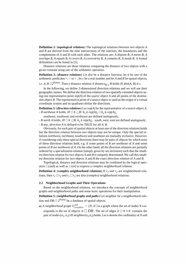
Definition 6: (filter starlike) Let p = [n1,n2,...,nk] be a neighborhood path and let reli be

the exact direction for ni and ni+1, i.e. ni+1 reli ni holds. The predicates starlike and var-

iable-starlike for paths p are defined as follows: starlike(p) :⇔ (∃ j < k: ∀ i > j: ni+1 reli ni ⇔ reli ⊆ relj), if k > 1; TRUE, if k=1.

ni N 1 i k<≤,∈

nge

te

uni-then

tions.x-enta-cted ahe ac-tabaseined

e

fhe

bjects.rgeathsumber

s isressed

lass-hereas

plica-roup-

The filter starlike requires that, when extending apath p, the exact “final” direction relj of p cannot begeneralized. For instance, a path with “final” directionortheast can only be extended by a node of an edwith exact direction northeast but not by an edge withexact direction north.Under the following assumptions, we can calcula

the number of all starlike neighborhood paths of a certain length l for a given fanout fof the neighborhood graph. Lemma 2: Let A be a spatial object and let l be an integer. Let intersects be chosen asthe neighborhood relation. If the representative points of all spatial objects areformly distributed and if they have the same extension in both x and y direction, the number of all starlike neighborhood paths with source A having a length of at most

l is O(2l) for f = 12 and O(l) for f = 6. (see [6] for a proof)The assumptions of this lemma may seem to be too restrictive for real applica

Note, however, that intersects is a very natural neighborhood relation for spatially etended objects. To evaluate the assumptions of uniform distribution of the represtive points of the spatial objects and of the same size of these objects, we conduset of experiments to compare the expected numbers of neighborhood paths with ttual number of paths created from a real geographic database on Bavaria. The dacontains the ATKIS 500 data [2] and the Bavarian part of the statistical data obtaby the German census of 1987.

We find that for f = 6 the number of all neighborhood paths (starting from the samsource) with a length of at most max-length is O(6max-length) and the number of the star-like neighborhood paths only grows approximately linear with increasing max-length -as stated by lemma 2. For f = 12 the number of all neighborhood paths with a length oat most max-length is O(12max-length) as we can expect from the lemma. However, tnumber of the starlike neighborhood paths is significantly less than O(2max-length). Thiseffect can be explained as follows. The lemma assumes equal size of the spatial oHowever, small destination objects are more likely to fulfil the filter starlike than ladestination objects implying that the size of objects on starlike neighborhood ptends to decrease. Note that lemma 2 nevertheless yields an upper bound for the nof starlike neighborhood paths created.

3 Algorithms for Spatial Data Mining

To support our claim that the expressivity of our spatial data mining primitiveadequate, we demonstrate how typical spatial data mining algorithms can be expby the database primitives introduced in section 2.

3.1 Spatial ClusteringClustering is the task of grouping the objects of a database into meaningful subc

es (that is, clusters) so that the members of a cluster are as similar as possible wthe members of different clusters differ as much as possible from each other. Aptions of clustering in spatial databases are, e.g., the detection of seismic faults by g

Fig. 2. Illustration of two different filter predicates

starlike

ensi- of a

d, in-res toance-y be

set

r thee rel-s. For

ing the entries of an earthquake catalog or the creation of thematic maps in geographicinformation systems by clustering feature spaces.

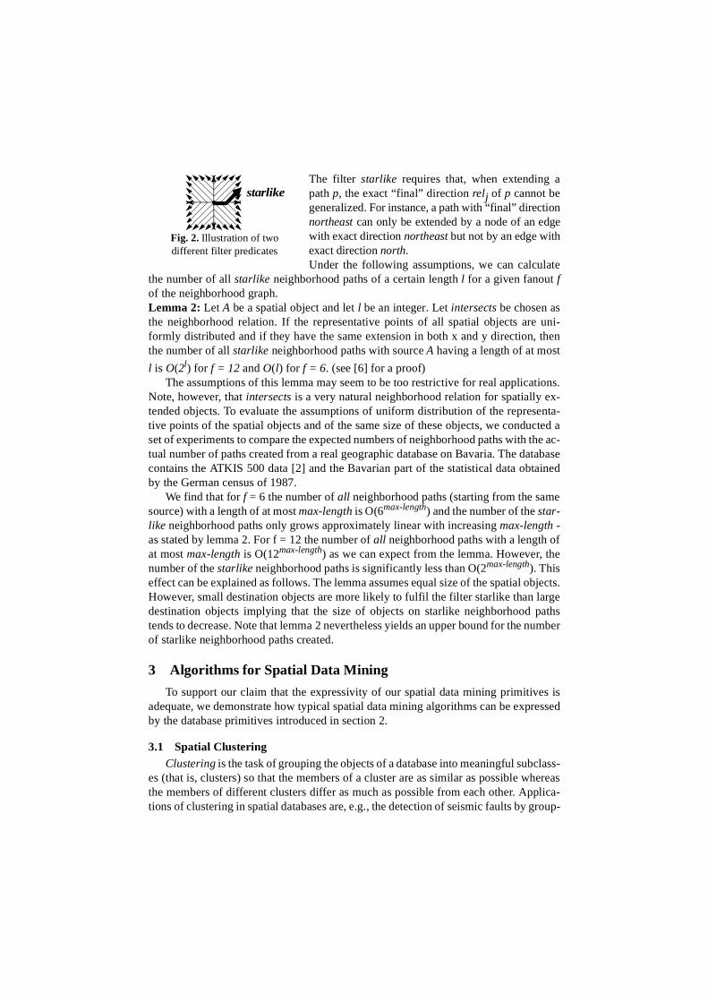
Different types of spatial clustering algorithms have been proposed. The basic ideaof a single scan algorithm is to group neighboring objects of the database into clustersbased on a local cluster condition performing only one scan through the database. Sin-gle scan clustering algorithms are efficient if the retrieval of the neighborhood of an ob-ject can be efficiently performed by the SDBS. Note that local cluster conditions arewell supported by the neighbors operation on an appropriate neighborhood graph.The algorithmic schema of single scan clustering is depicted in figure 3.

Different cluster conditions yield different notions of a cluster and different cluster-ing algorithms. For example, GDBSCAN [16] relies on a density-based notion of clus-ters. The key idea of a density-based cluster is that for each point of a cluster its ε-neighborhood has to contain at least a minimum number of points. This idea of “dty-based clusters” can be generalized in two important ways. First, any notionneighborhood can be used instead of an ε-neighborhood if the definition of the neigh-borhood is based on a binary predicate which is symmetric and reflexive. Seconstead of simply counting the objects in a neighborhood of an object other measudefine the “cardinality” of that neighborhood can be used as well. Whereas a distbased neighborhood is a natural notion of a neighborhood for point objects, it mamore appropriate to use topological relations such as intersects or meets to cluster spa-tially extended objects such as a set of polygons of largely differing sizes.

3.2 Spatial Characterization

The task of characterization is to find a compact description for a selected sub(the target set) of the database. A spatial characterization [8] is a description of the spa-tial and non-spatial properties which are typical for the target objects but not fowhole database. The relative frequencies of the non-spatial attribute values and thative frequencies of the different object types are used as the interesting propertie

SingleScanClustering(Database db; NRelation rel)set Graph to create_NGraph(db,rel);initialize a set CurrentObjects as empty;for each node O in Graph do

if O is not yet member of some cluster thencreate a new cluster C;insert O into CurrentObjects;while CurrentObjects not empty do

remove the first element of CurrentObjects as O;set Neighbors to neighbors(Graph, O, TRUE);if Neighbors satisfy the cluster condition do

add O to cluster C;add Neighbors to CurrentObjects;

end SingleScanClustering;Fig. 3. Schema of single scan clustering algorithms

GH”ts, si- val-.

de-butesr the

hen

ive at-ty off-e cor-ssion

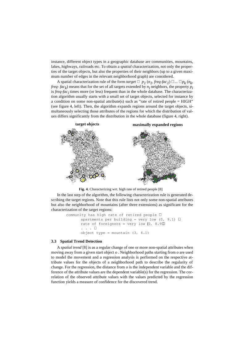
instance, different object types in a geographic database are communities, mountains,lakes, highways, railroads etc. To obtain a spatial characterization, not only the proper-ties of the target objects, but also the properties of their neighbors (up to a given maxi-mum number of edges in the relevant neighborhood graph) are considered.

A spatial characterization rule of the form target ⇒ p1 (n1, freq-fac1) ∧ ... ∧ pk (nk,freq- fack) means that for the set of all targets extended by ni neighbors, the property piis freq-faci times more (or less) frequent than in the whole database. The characteriza-tion algorithm usually starts with a small set of target objects, selected for instance bya condition on some non-spatial attribute(s) such as “rate of retired people = HI(see figure 4, left). Then, the algorithm expands regions around the target objecmultaneously selecting those attributes of the regions for which the distribution ofues differs significantly from the distribution in the whole database (figure 4, right)

In the last step of the algorithm, the following characterization rule is generatedscribing the target regions. Note that this rule lists not only some non-spatial attribut also the neighborhood of mountains (after three extensions) as significant focharacterization of the target regions:

community has high rate of retired people ⇒ apartments per building = very low (0, 9.1) ∧ rate of foreigners = very low (0, 8.9) ∧ . . . ∧ object type = mountain (3, 4.1)

3.3 Spatial Trend Detection

A spatial trend [8] is as a regular change of one or more non-spatial attributes wmoving away from a given start object o . Neighborhood paths starting from o are usedto model the movement and a regression analysis is performed on the respecttribute values for the objects of a neighborhood path to describe the regularichange. For the regression, the distance from o is the independent variable and the diference of the attribute values are the dependent variable(s) for the regression. Threlation of the observed attribute values with the values predicted by the regrefunction yields a measure of confidence for the discovered trend.

Fig. 4. Characterizing wrt. high rate of retired people [8]

maximally expanded regionstarget objects

ty of

-right)t rep-

peeds [10].fbjectigh-paths

es onevantay be

t deal joinis in-ringance

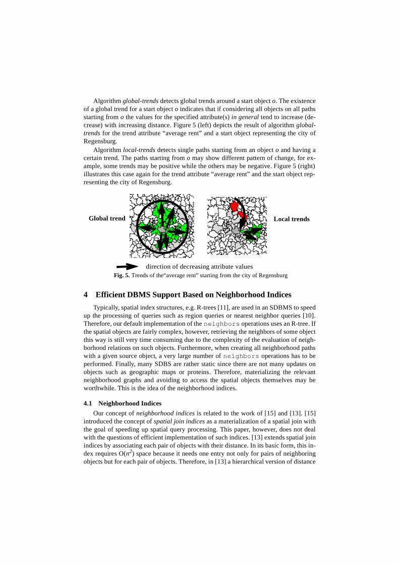
Algorithm global-trends detects global trends around a start object o. The existenceof a global trend for a start object o indicates that if considering all objects on all pathsstarting from o the values for the specified attribute(s) in general tend to increase (de-crease) with increasing distance. Figure 5 (left) depicts the result of algorithm global-trends for the trend attribute “average rent” and a start object representing the ciRegensburg.

Algorithm local-trends detects single paths starting from an object o and having acertain trend. The paths starting from o may show different pattern of change, for example, some trends may be positive while the others may be negative. Figure 5 (illustrates this case again for the trend attribute “average rent” and the start objecresenting the city of Regensburg.

4 Efficient DBMS Support Based on Neighborhood Indices

Typically, spatial index structures, e.g. R-trees [11], are used in an SDBMS to sup the processing of queries such as region queries or nearest neighbor querieTherefore, our default implementation of the neighbors operations uses an R-tree. Ithe spatial objects are fairly complex, however, retrieving the neighbors of some othis way is still very time consuming due to the complexity of the evaluation of neborhood relations on such objects. Furthermore, when creating all neighborhood with a given source object, a very large number of neighbors operations has to beperformed. Finally, many SDBS are rather static since there are not many updatobjects such as geographic maps or proteins. Therefore, materializing the relneighborhood graphs and avoiding to access the spatial objects themselves mworthwhile. This is the idea of the neighborhood indices.

4.1 Neighborhood Indices

Our concept of neighborhood indices is related to the work of [15] and [13]. [15]introduced the concept of spatial join indices as a materialization of a spatial join withthe goal of speeding up spatial query processing. This paper, however, does nowith the questions of efficient implementation of such indices. [13] extends spatialindices by associating each pair of objects with their distance. In its basic form, thdex requires O(n2) space because it needs one entry not only for pairs of neighboobjects but for each pair of objects. Therefore, in [13] a hierarchical version of dist

Fig. 5. Trends of the“average rent” starting from the city of Regensburg

Global trend Local trends

direction of decreasing attribute values

eigh-

tion,

. We-s ap-

ance

associated join indices is proposed. In general, however, we cannot rely on such hierar-chies for the purpose of supporting spatial data mining. Our approach, called neighbor-hood indices, extends distance associated join indices with the following newcontributions:• A specified maximum distance restricts the pairs of objects represented in a n

borhood index.• For each of the different types of neighborhood relations (that is distance, direc

and topological relations), the concrete relation of the pair of objects is stored.

Definition 7: (neighborhood index) Let DB be a set of spatial objects and let max anddist be real numbers. Let D be a direction relation and T be a topological relation. Then

the neighborhood index for DB with maximum distance max, denoted by , is de-

fined as follows: = {(O1,O2,dist,D,T) | O1, O2 ∈ DB ∧ O1 distance=dist O2 ∧ dist ≤ max ∧ O2 D O1 ∧ O1 T O2}.

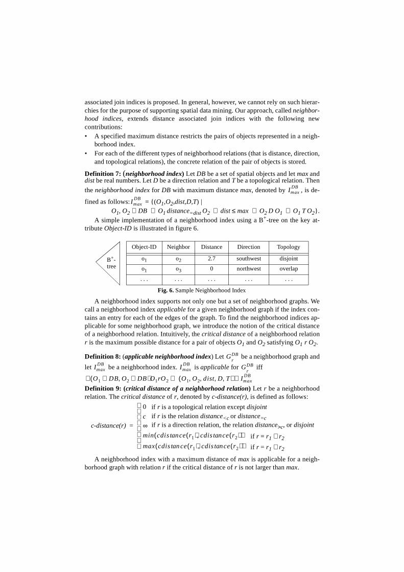
A simple implementation of a neighborhood index using a B+-tree on the key at-tribute Object-ID is illustrated in figure 6.

A neighborhood index supports not only one but a set of neighborhood graphscall a neighborhood index applicable for a given neighborhood graph if the index contains an entry for each of the edges of the graph. To find the neighborhood indiceplicable for some neighborhood graph, we introduce the notion of the critical distof a neighborhood relation. Intuitively, the critical distance of a neighborhood relationr is the maximum possible distance for a pair of objects O1 and O2 satisfying O1 r O2.

Definition 8: (applicable neighborhood index) Let be a neighborhood graph and

let be a neighborhood index. is applicable for iff

Definition 9: (critical distance of a neighborhood relation) Let r be a neighborhoodrelation. The critical distance of r, denoted by c-distance(r), is defined as follows:

A neighborhood index with a maximum distance of max is applicable for a neigh-borhood graph with relation r if the critical distance of r is not larger than max.

ImaxDB

ImaxDB

Object-ID Neighbor Distance Direction Topology

o1 o2 2.7 southwest disjoint

o1 o3 0 northwest overlap

. . . . . . . . . . . . . . .

B+-tree

Fig. 6. Sample Neighborhood Index

GDBr

ImaxDB Imax

DB GDBr

O1 DB∈ O2 DB∈,( )O1rO2∀ O1 O2 dist D T, , , ,( ) ImaxDB∈⇒

c-distance(r)

0

c

∞min cdis ce r1( ) cdis ce r2( )tan,tan( )max cdis ce r1( ) cdis ce r2( )tan,tan( )

=

if r is a topological relation except disjointif r is the relation distance<c or distance=cif r is a direction relation, the relation distance>c, or disjoint

if r = r1 ∧ r2

if r = r1 ∨ r2

Lemma 3: Let be a neighborhood graph and let be a neighborhood index.

If max ≥ c-distance(r), then is applicable for .

Obviously, if two neighborhood indices and with c1 < c2 are available andapplicable, using is more efficient because in general it has less entries than .The smallest applicable neighborhood index for some neighborhood graph is the appli-cable neighborhood index with the smallest critical distance.

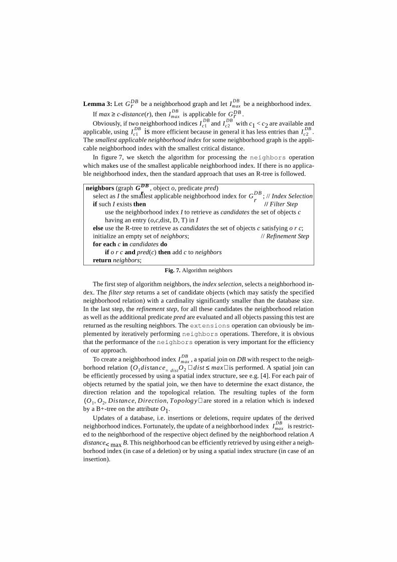
In figure 7, we sketch the algorithm for processing the neighbors operationwhich makes use of the smallest applicable neighborhood index. If there is no applica-ble neighborhood index, then the standard approach that uses an R-tree is followed.

The first step of algorithm neighbors, the index selection, selects a neighborhood in-dex. The filter step returns a set of candidate objects (which may satisfy the specifiedneighborhood relation) with a cardinality significantly smaller than the database size.In the last step, the refinement step, for all these candidates the neighborhood relationas well as the additional predicate pred are evaluated and all objects passing this test arereturned as the resulting neighbors. The extensions operation can obviously be im-plemented by iteratively performing neighbors operations. Therefore, it is obviousthat the performance of the neighbors operation is very important for the efficiencyof our approach.

To create a neighborhood index , a spatial join on DB with respect to the neigh-borhood relation is performed. A spatial join canbe efficiently processed by using a spatial index structure, see e.g. [4]. For each pair ofobjects returned by the spatial join, we then have to determine the exact distance, thedirection relation and the topological relation. The resulting tuples of the form

are stored in a relation which is indexedby a B+-tree on the attribute O1.

Updates of a database, i.e. insertions or deletions, require updates of the derivedneighborhood indices. Fortunately, the update of a neighborhood index is restrict-ed to the neighborhood of the respective object defined by the neighborhood relation Adistance< max B. This neighborhood can be efficiently retrieved by using either a neigh-borhood index (in case of a deletion) or by using a spatial index structure (in case of aninsertion).

GDBr Imax

DB

ImaxDB

GDBr

Ic1DB

Ic2DB

Ic1DB

Ic2DB

neighbors (graph , object o, predicate pred)select as I the smallest applicable neighborhood index for ; // Index Selectionif such I exists then // Filter Step

use the neighborhood index I to retrieve as candidates the set of objects c having an entry (o,c,dist, D, T) in I

else use the R-tree to retrieve as candidates the set of objects c satisfying o r c;initialize an empty set of neighbors; // Refinement Stepfor each c in candidates do

if o r c and pred(c) then add c to neighborsreturn neighbors;

GDB

r GDB

r

Fig. 7. Algorithm neighbors

ImaxDB

O1dis cetan dist= O2 dist max≤∧( )

O1 O2 Dis cetan Direction Topo ylog, , , ,( )

ImaxDB

4.2 Cost ModelWe developed a cost model to predict the cost of performing a neighbors opera-

tion with and without a neighborhood index. We use tpage, i.e. the execution time of apage access, and tfloat, i.e. the execution time of a floating point comparison, as the unitsfor I/O time and CPU time, respectively.

In table 1, we define the parameters of the cost model and list typical values for eachof them. The system overhead s includes client-server communication and the overheadinduced by several SQL queries for retrieving the relevant neighborhood index and theminimum bounding box of a polygon (necessary for the access of the R-tree). pindex andpdata denote the probability that a requested index page and data page, respectively,have to be read from disk according to the buffering strategy.

Table 2 shows the cost for the three steps of processing a neighbors operationwith and without a neighborhood index. In the R-tree, there is one entry for each of then nodes of the neighborhood graph whereas the B+-tree stores one entry for each of thef * n edges. We assume that the number of R-tree paths to be followed is proportionalto the number of neighboring objects, i.e. proportional to f. A spatial object with v ver-tices requires v/cv data pages. We assume a distance relation as neighborhood relationrequiring v2 floating point comparisons. When using a neighborhood index, the filterstep returns ff * f candidates. The refinement step has to access their index entries butdoes not have to access the vertices of the candidates since the refinement test can bedirectly performed by using the attributes Distance, Direction and Topology of the indexentries. This test involves a constant (i.e. independent of v) number of floating pointcomparisons and requires no page accesses implying that its cost can be neglected.

Table 1: Parameters of the cost model

name meaning typical values

n number of nodes in the neighborhood graph [103 . . 105]

f average number of edges per node in the graph (fan out) [1 . . 102]

v average number of vertices of a spatial object [1 . . 103]

ff ratio of fanout of the index and fanout (f) of the graph [1 . . 10]

cindex capacity of a page in terms of index entries 128

cv capacity of a page in terms of vertices 64

pindex probability that a given index page must be read from disk [0..1]

pdata probability that a given data page must be read from disk [0..1]

tpage average execution time for a page access 1 * 10-2 sec

tfloat execution time for a floating point comparison 3 * 10-6 sec

s system overhead depends on DBMS

4.3 Experimental Results

We implemented the database primitives on top of the commercial DBMS Illustrausing its 2D spatial data blade which provides R-trees. A geographic database of Bavar-ia was used for an experimental performance evaluation and validation of the cost mod-el. This database represents the Bavarian communities with one spatial attribute(polygon) and 52 non-spatial attributes (such as average rent or rate of unemployment).All experiments were run on HP9000/715 (50MHz) workstations under HP-UX 10.10.

The first set of experiments compared the performance predicted by our cost modelswith the experimental performance when varying the parameters n, f and v. The resultsshow that our cost model is able to predict the performance reasonably well. For in-stance, figure 8 depicts the results for n = 2,000, v = 35 and varying values for f.

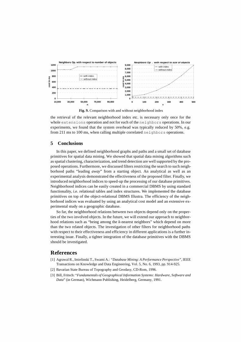
We used our cost model to compare the performance of the neighbors operationwith and without neighborhood index for combinations of parameter values which wecould not evaluate experimentally with our database. Figure 9 depicts the results (1) forf = 10, v = 100 and varying n and (2) for n = 100,000, f = 10 and varying v. These resultsdemonstrate a significant speed-up for the neighbors operation with compared towithout neighborhood index. Furthermore, this speed-up grows strongly with increas-ing number of vertices of the spatial objects.

The next set of experiments analyzed the system overhead which is rather large.This overhead, however, can be reduced when calling multiple correlated neighbors op-erations issued by one extensions operation, since the client-server communication,

Table 2: Cost model for the neighbors operation

Step Cost without neighborhood index Cost with neighborhood index

Selec-tion

s s

Filter

Refine-ment

f logcindexn pindex⋅ ⋅ tpage⋅ logcindex

f n⋅( ) pindex⋅ tpage⋅

1 f+( ) v cv⁄ pdata⋅ ⋅ tpage⋅ f v2

tfloat⋅ ⋅+ ff f pdata⋅ ⋅ tpage⋅

Fig. 8. Comparison of cost model versus experimental results

Comparison without index

600

625

650

675

700

725

2 3 4 5 6 7f

cost

in m

s

modelexperiments

Comparison with index

240

250

260

270

280

290

2 3 4 5 6 7f

cost

in m

s

modelexperiments

nly, weitives.dard

oper-bor-reathsr in-MS

the retrieval of the relevant neighborhood index etc. is necessary only once for thewhole extensions operation and not for each of the neighbors operations. In ourexperiments, we found that the system overhead was typically reduced by 50%, e.g.from 211 ms to 100 ms, when calling multiple correlated neighbors operations.

5 Conclusions

In this paper, we defined neighborhood graphs and paths and a small set of databaseprimitives for spatial data mining. We showed that spatial data mining algorithms suchas spatial clustering, characterization, and trend detection are well supported by the pro-posed operations. Furthermore, we discussed filters restricting the search to such neigh-borhood paths “leading away” from a starting object. An analytical as well as aexperimental analysis demonstrated the effectiveness of the proposed filter. Finalintroduced neighborhood indices to speed-up the processing of our database primNeighborhood indices can be easily created in a commercial DBMS by using stanfunctionality, i.e. relational tables and index structures. We implemented the databaseprimitives on top of the object-relational DBMS Illustra. The efficiency of the neigh-borhood indices was evaluated by using an analytical cost model and an extensive ex-perimental study on a geographic database.

So far, the neighborhood relations between two objects depend only on the prties of the two involved objects. In the future, we will extend our approach to neighhood relations such as “being among the k-nearest neighbors” which depend on mothan the two related objects. The investigation of other filters for neighborhood pwith respect to their effectiveness and efficiency in different applications is a furtheteresting issue. Finally, a tighter integration of the database primitives with the DBshould be investigated.

References[1] Agrawal R., Imielinski T., Swami A.: “Database Mining: A Performance Perspective”, IEEE

Transactions on Knowledge and Data Engineering, Vol. 5, No. 6, 1993, pp. 914-925.

[2] Bavarian State Bureau of Topography and Geodasy, CD-Rom, 1996.

[3] Bill, Fritsch: “Fundamentals of Geographical Information Systems: Hardware, Software andData” (in German), Wichmann Publishing, Heidelberg, Germany, 1991.

Neighbors Op . with respect to size of objects

0

1,000

2,000

3,000

4,000

5,000

6,000

7,000

8,000

9,000

0 100 200 300 400 500v

cost

in m

s

with indexwithout index

Neighbors Op. with respect to number of objects

0

200

400

600

800

1000

1200

10,000 30,000 50,000 70,000 90,000n

cost

in m

s with indexwithout index

Fig. 9. Comparison with and without neighborhood index

urg,

d

:

[4] Brinkhoff T., Kriegel H.-P., Schneider R., and Seeger B.: “Efficient Multi-Step Processing ofSpatial Joins”. Proc. ACM SIGMOD ’94, Minneapolis, MN, 1994, pp. 197-208.

[5] Egenhofer M. J.: “Reasoning about Binary Topological Relations”, Proc. 2nd Int. Symp. onLarge Spatial Databases, Zurich, Switzerland, 1991, pp. 143-160.

[6] Ester M., Gundlach S., Kriegel H.-P., Sander J.: “Database Primitives for Spatial DataMining”, Proc. Int. Conf. on Databases in Office, Engineering and Science (BTW'99), FreibGermany, 1999.

[7] Ester M., Kriegel H.-P., Sander J.: “Spatial Data Mining: A Database Approach”, Proc. 5thInt. Symp. on Large Spatial Databases, Berlin, Germany, 1997, pp. 47-66.

[8] Ester M., Frommelt A., Kriegel H.-P., Sander J.: “Algorithms for Characterization and TrendDetection in Spatial Databases”, Proc. 4th Int. Conf. on Knowledge Discovery and DataMining, New York City, NY, 1998, pp. 44-50.

[9] Fayyad U. M., .J., Piatetsky-Shapiro G., Smyth P.: “From Data Mining to KnowledgeDiscovery: An Overview”, in: Advances in Knowledge Discovery and Data Mining, AAAIPress, Menlo Park, 1996, pp. 1 - 34.

[10] Gueting R. H.: “An Introduction to Spatial Database Systems”, Special Issue on SpatialDatabase Systems of the VLDB Journal, Vol. 3, No. 4, October 1994.

[11] Guttman A.: “R-trees: A Dynamic Index Structure for Spatial Searching“, Proc. ACMSIGMOD ‘84, 1984, pp. 47-54.

[12] Koperski K., Adhikary J., Han J.: “Knowledge Discovery in Spatial Databases: Progress anChallenges”, Proc. SIGMOD Workshop on Research Issues in Data Mining and KnowledgeDiscovery, Technical Report 96-08, UBC, Vancouver, Canada, 1996.

[13] Lu W., Han J.: “Distance-Associated Join Indices for Spatial Range Search”, Proc. 8th Int.Conf. on Data Engineering, Phoenix, AZ, 1992, pp. 284-292.

[14] Ng R. T., Han J.:“Efficient and Effective Clustering Methods for Spatial Data Mining”, Proc.20th Int. Conf. on Very Large Data Bases, Santiago, Chile, 1994, pp. 144-155.

[15] Rotem D.: “Spatial Join Indices”, Proc. 7th Int. Conf. on Data Engineering, Kobe, Japan,1991, pp. 500-509.

[16] Sander J., Ester M., Kriegel H.-P., Xu X.: “Density-Based Clustering in Spatial DatabasesA New Algorithm and its Applications”, Data Mining and Knowledge Discovery, anInternational Journal, Kluwer Academic Publishers, Vol.2, No. 2, 1998.