lab manual heat transfer iii b. tech ii...
TRANSCRIPT

HEAT TRANSFER LAB Page 1
LAB MANUAL
HEAT TRANSFER
III B. TECH II SEM
HEAT TRANSFER LAB Page 2
DEPARTMENT
OF
MECHANICAL ENGINEERING
NAME OF THE LABORATORY : HEAT TRANSFER
YEAR & SEM : IV B.TECH I SEM
LAB CODE : ME604PC
HOD PRINCIPAL
HEAT TRANSFER LAB Page 3
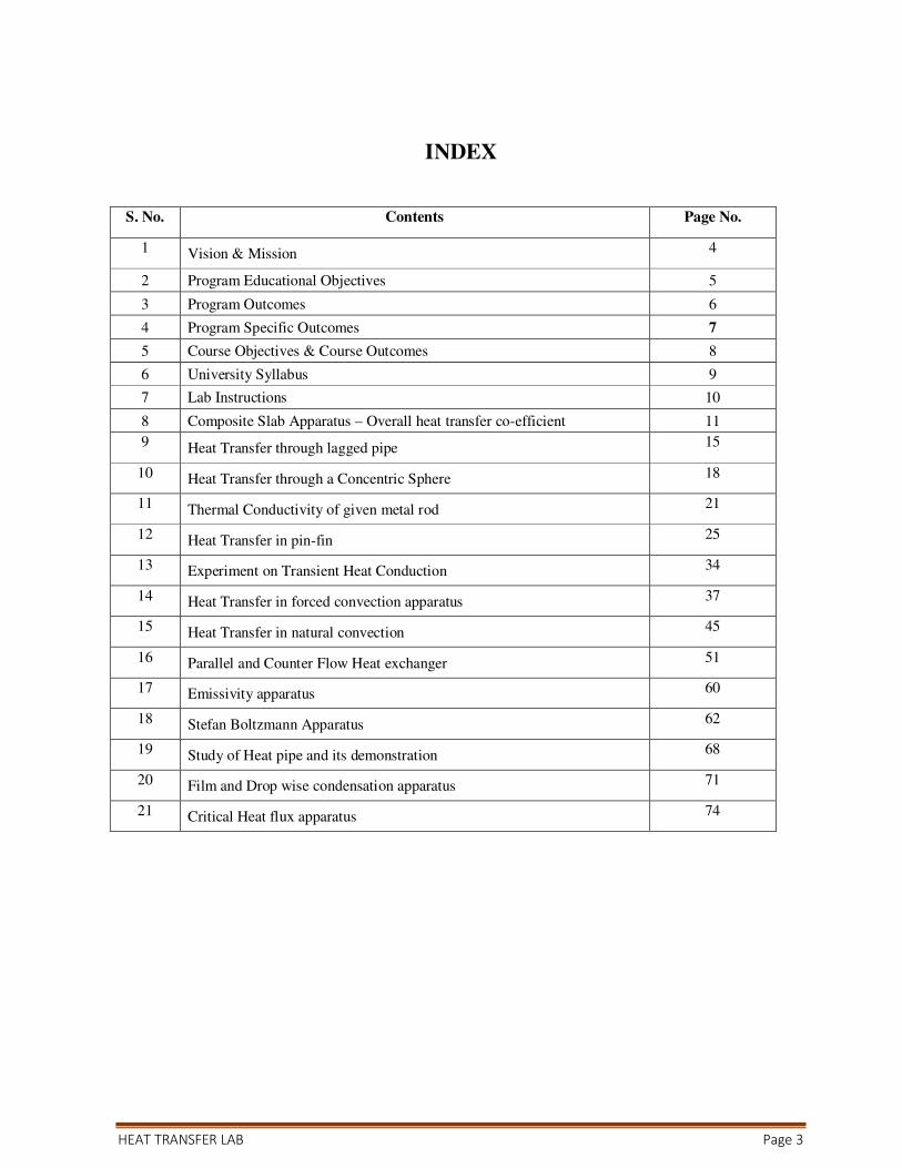
INDEX
S. No. Contents Page No.
1 Vision & Mission 4
2 Program Educational Objectives 5
3 Program Outcomes 6
4 Program Specific Outcomes 7
5 Course Objectives & Course Outcomes 8
6 University Syllabus 9
7 Lab Instructions 10
8 Composite Slab Apparatus – Overall heat transfer co-efficient 11
9 Heat Transfer through lagged pipe 15
10 Heat Transfer through a Concentric Sphere 18
11 Thermal Conductivity of given metal rod 21
12 Heat Transfer in pin-fin 25
13 Experiment on Transient Heat Conduction 34
14 Heat Transfer in forced convection apparatus 37
15 Heat Transfer in natural convection 45
16 Parallel and Counter Flow Heat exchanger 51
17 Emissivity apparatus 60
18 Stefan Boltzmann Apparatus 62
19 Study of Heat pipe and its demonstration 68
20 Film and Drop wise condensation apparatus 71
21 Critical Heat flux apparatus 74

HEAT TRANSFER LAB Page 4
VISION & MISSION
VISION
Mechanical Engineering Department of KG REDDY College of Engineering & Technology strives to
be recognized globally for imparting outstanding technical education and research leading to well
qualified truly world class leaders and unleashes technological innovations to serve the global society
with an ultimate aim to improve the quality of life.
MISSION
Mechanical Engineering Department of KGRCET strives to create world class Mechanical Engineers
by:
Imparting quality education to its students and enhancing their skills.
Encouraging innovative research and consultancy by establishing the state of the art research
facilities through which the faculty members and engineers from the nearby industries can actively
utilize the established the research laboratories.
Expanding curricula as appropriate to include broader prospective.
Establishing linkages with world class R&D organizations and leading educational institutions in
India and abroad for excelling in teaching, research and consultancy.
Creation of service opportunities for the up-liftment of society at large.

HEAT TRANSFER LAB Page 5
PROGRAM EDUCATIONAL OBJECTIVES (PEO’S)
PEOs Description
PEO1 To apply deep working knowledge of technical fundamentals in areas related to thermal,
production, design, materials, system engineering areas of Mechanical Engineering.
PEO2 To develop innovative ideas and fine solutions to various mechanical engineering problems.
PEO3 To communicate effectively as members of multidisciplinary teams.
PEO4 To be sensitive to professional and societal context and committed to ethical action.
PEO5 To lead in the conception, design and implementation of new products, processes, services
and systems.
HEAT TRANSFER LAB Page 6
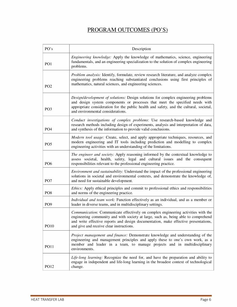
PROGRAM OUTCOMES (PO’S)
PO’s Description
PO1
Engineering knowledge: Apply the knowledge of mathematics, science, engineering
fundamentals, and an engineering specialization to the solution of complex engineering
problems.
PO2
Problem analysis: Identify, formulate, review research literature, and analyze complex
engineering problems reaching substantiated conclusions using first principles of
mathematics, natural sciences, and engineering sciences.
PO3
Design/development of solutions: Design solutions for complex engineering problems
and design system components or processes that meet the specified needs with
appropriate consideration for the public health and safety, and the cultural, societal,
and environmental considerations.
PO4
Conduct investigations of complex problems: Use research-based knowledge and
research methods including design of experiments, analysis and interpretation of data, and synthesis of the information to provide valid conclusions.
PO5
Modern tool usage: Create, select, and apply appropriate techniques, resources, and
modern engineering and IT tools including prediction and modelling to complex
engineering activities with an understanding of the limitations.
PO6
The engineer and society: Apply reasoning informed by the contextual knowledge to
assess societal, health, safety, legal and cultural issues and the consequent
responsibilities relevant to the professional engineering practice.
PO7
Environment and sustainability: Understand the impact of the professional engineering
solutions in societal and environmental contexts, and demonstrate the knowledge of,
and need for sustainable development.
PO8
Ethics: Apply ethical principles and commit to professional ethics and responsibilities
and norms of the engineering practice.
PO9
Individual and team work: Function effectively as an individual, and as a member or
leader in diverse teams, and in multidisciplinary settings.
PO10
Communication: Communicate effectively on complex engineering activities with the engineering community and with society at large, such as, being able to comprehend
and write effective reports and design documentation, make effective presentations,
and give and receive clear instructions.
PO11
Project management and finance: Demonstrate knowledge and understanding of the
engineering and management principles and apply these to one’s own work, as a
member and leader in a team, to manage projects and in multidisciplinary
environments.
PO12
Life-long learning: Recognize the need for, and have the preparation and ability to engage in independent and life-long learning in the broadest context of technological
change.

HEAT TRANSFER LAB Page 7
PROGRAM SPECIFIC OUTCOMES (PSO’S)
PSO’s Description
PSO 1 Apply the knowledge in the domain of engineering mechanics, thermal and fluid sciences to
solve engineering problems utilizing advanced technology.
PSO 2 Successfully evaluates the principle of design, analysis and implementation of mechanical
systems / processes which have been learned as a part of the curriculum.
PSO 3 Develop and implement new ideas on product design and development with the help of
modern CAD / CAM tools, while ensuring best manufacturing practices.
HEAT TRANSFER LAB Page 8
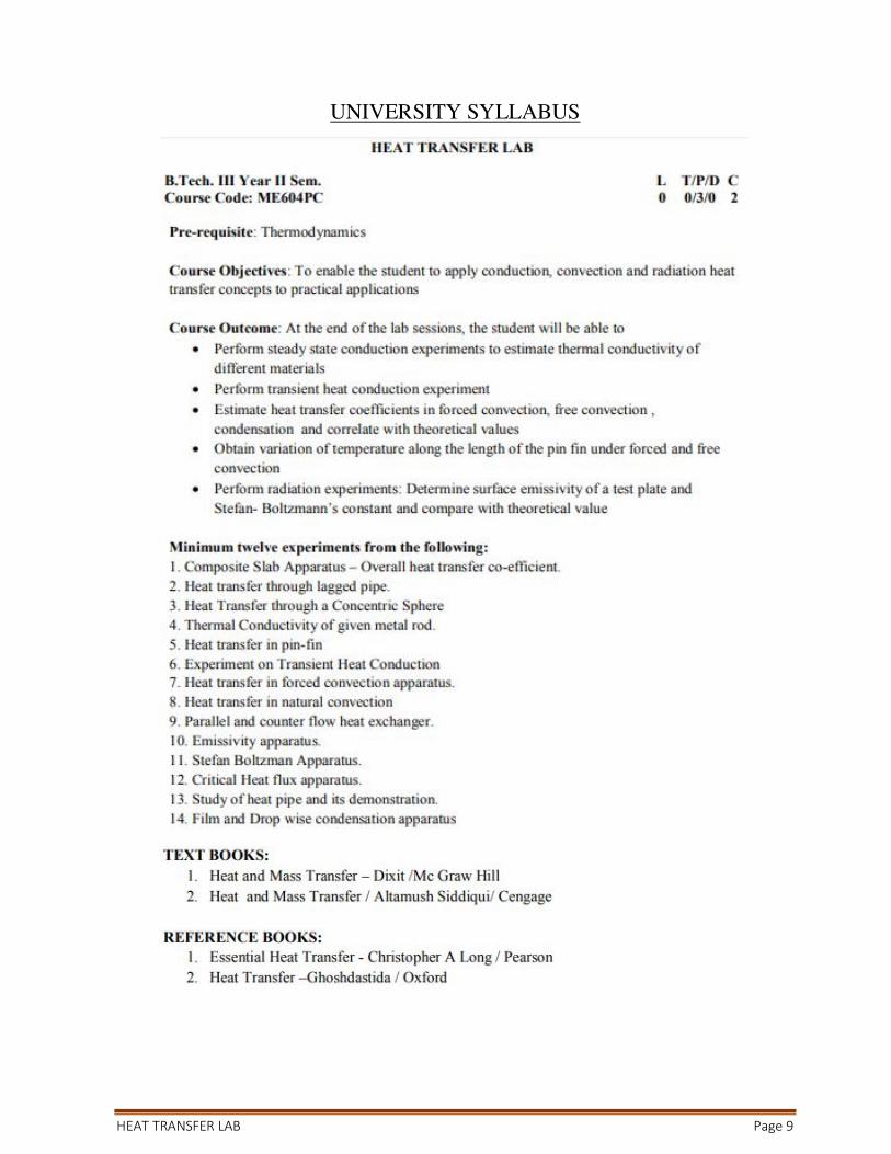
COURSE OBJECTIVES & COURSE OUTCOMES
HEAT TRANSFER LAB Page 9
UNIVERSITY SYLLABUS
HEAT TRANSFER LAB Page 10
LAB INSTRUCTIONS
1. Laboratory uniform, shoes are compulsory in the lab.
2. Student should wear college ID-card and must carry record and observation.
3. Take signature of lab in charge after completion of observation and record.
4. If any equipment fails in the experiment report it to the supervisor immediately.
5. Students should come to the lab with thorough theoretical knowledge.
6. Don't touch the equipment without instructions from lab supervisor.
7. Don't crowd around the experiment and behave in-disciplinary.
8. Students should carry their own stationary and required things.
9. Using the mobile phone in the laboratory is strictly prohibited.
HEAT TRANSFER LAB Page 11
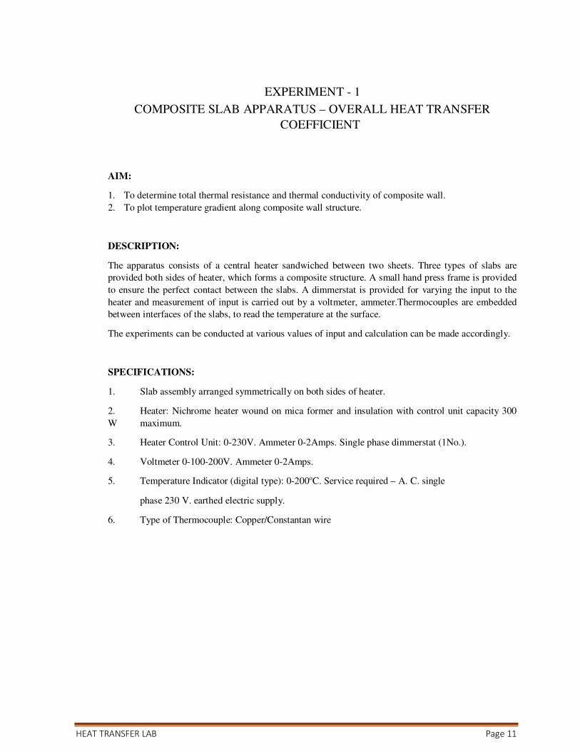
EXPERIMENT - 1
COMPOSITE SLAB APPARATUS – OVERALL HEAT TRANSFER
COEFFICIENT
AIM:
1. To determine total thermal resistance and thermal conductivity of composite wall.
2. To plot temperature gradient along composite wall structure.
DESCRIPTION:
The apparatus consists of a central heater sandwiched between two sheets. Three types of slabs are
provided both sides of heater, which forms a composite structure. A small hand press frame is provided
to ensure the perfect contact between the slabs. A dimmerstat is provided for varying the input to the
heater and measurement of input is carried out by a voltmeter, ammeter.Thermocouples are embedded
between interfaces of the slabs, to read the temperature at the surface.
The experiments can be conducted at various values of input and calculation can be made accordingly.
SPECIFICATIONS:
1. Slab assembly arranged symmetrically on both sides of heater.
2. Heater: Nichrome heater wound on mica former and insulation with control unit capacity 300
W maximum.
3. Heater Control Unit: 0-230V. Ammeter 0-2Amps. Single phase dimmerstat (1No.).
4. Voltmeter 0-100-200V. Ammeter 0-2Amps.
5. Temperature Indicator (digital type): 0-200oC. Service required – A. C. single
phase 230 V. earthed electric supply.
6. Type of Thermocouple: Copper/Constantan wire

HEAT TRANSFER LAB Page 12
SCHEMATIC DIAGRAM:
(11) Thermocouple Socket (T1 To T6 Thermocouple Positions)
(1) Hand Wheel (2) Screw
(3) Cabinet (4) Fabricated Frame
(5) Acrylic Sheet (6) Press Wood Plate
(7) Bakelite Plate (8) C.I. Plate
(9) Heater (10) Heater Cable

HEAT TRANSFER LAB Page 13
SAMPLE CALCULATIONS:
Determine the unknown thermal conductivity of press wood:
Total amount of heat delivered to the slab = 40 W
Since the heater is positioned at the center and similar slabs are fixed on either side. Therefore, amount
of heat transferred to the RHS portion of the composite slab will be
4020
2Q W= =
1T 126= , 2T 123= , 3T 82= , 4T 80= , 5T 60= , 6T 59=
( )1 5T T T 126 60 66∆ = − = − =
1x 12mm 0.012m= = ; o1k 52W /m C= − (cast iron)
2x 12mm 0.012m= = ; o2k 1.4W /m C= − (bakelite)
3x 12mm 0.012m= = ; o3k ? W /m C= − (press wood)
Heat transfer area (i.e. area of the slab perpendicular to the direction of heat flow)
2 22D 3.17 0.15
A 0.0177m4 4
π ×= = =
Heat flux, 2Q 1
q 1130W/mA 0.0177
= = =
3 1 2
3 1 2
x x xT
K q K K
∆= − +
( )3
0.0125 66 0.0125 0.0125
K 1130 52 4= − +
3K 0.24W / m C= −�
Literature value of thermal conductivity of press wood lies between 0.1 & 0.27 W/m-oC

HEAT TRANSFER LAB Page 14
Composite Wall Apparatus
Plate Diameter (m) Thickness (m) Area (m2) Thermal
Conductivity
Cast Iron 0.15 0.0125 0.000127 82
Bakelite 0.15 0.0125 0.000127 1.4
Press Wood 0.15 0.0125 0.000127 0.12
CALCULATION FOR K3 PRESSWOOD VALUE
S. No.
Heat Input
T1 T2 T3 T4 T5 T6 3 1 2
3 1 2
x x xT
K q K K
∆= − +
V I Q = V x I
EXAMPLE 1 220 0.18 40 126 125 93 91 60 58 3K 0.24W / m C= −�
EXAMPLE 2
1
2
HEAT TRANSFER LAB Page 15
EXPERIMENT – 2
HEAT TRANSFER THROUGH LAGGED PIPE
AIM:
1. To determine heat flow rate through the lagged pipe and compare it with the heater for known value of
thermal conductivity of lagging material.
2. To determine the thermal conductivity of lagging material by assuming the heater input to be the heat
flow rate through lagged pipe.
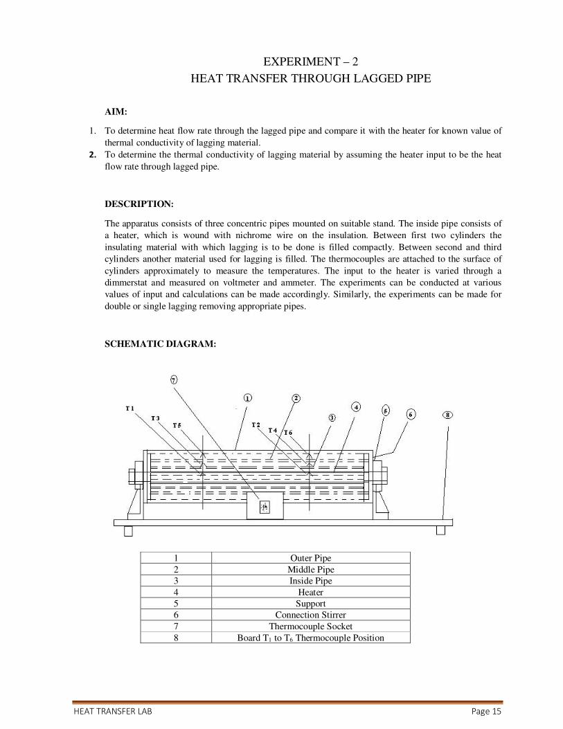
DESCRIPTION:
The apparatus consists of three concentric pipes mounted on suitable stand. The inside pipe consists of
a heater, which is wound with nichrome wire on the insulation. Between first two cylinders the
insulating material with which lagging is to be done is filled compactly. Between second and third
cylinders another material used for lagging is filled. The thermocouples are attached to the surface of
cylinders approximately to measure the temperatures. The input to the heater is varied through a
dimmerstat and measured on voltmeter and ammeter. The experiments can be conducted at various
values of input and calculations can be made accordingly. Similarly, the experiments can be made for
double or single lagging removing appropriate pipes.
SCHEMATIC DIAGRAM:
1 Outer Pipe
2 Middle Pipe
3 Inside Pipe
4 Heater
5 Support
6 Connection Stirrer
7 Thermocouple Socket
8 Board T1 to T6 Thermocouple Position
HEAT TRANSFER LAB Page 16
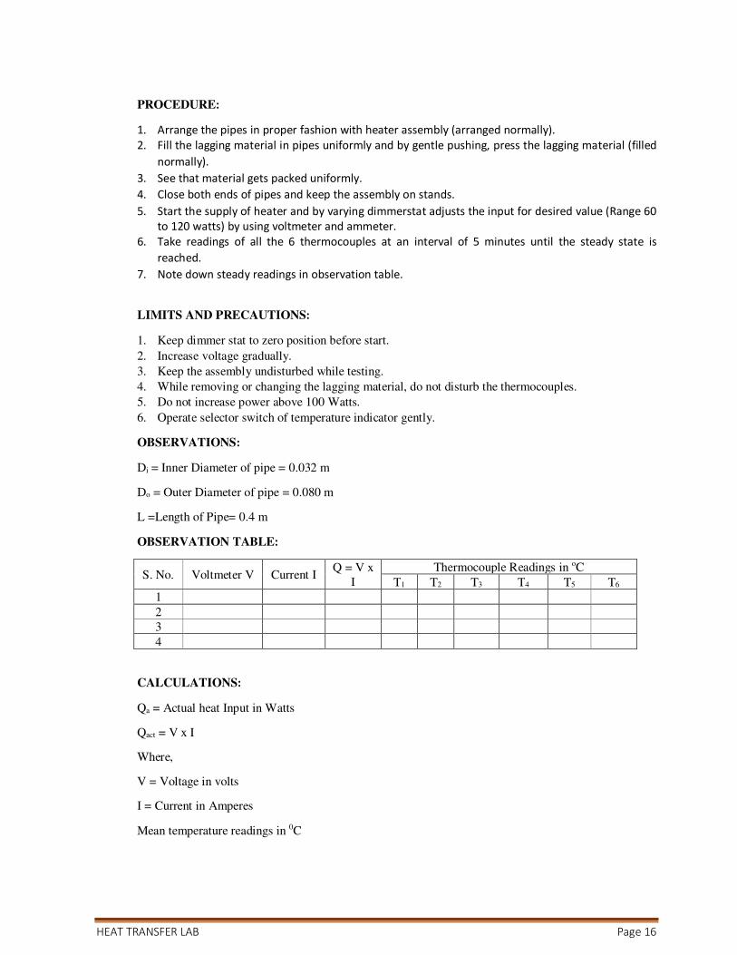
PROCEDURE:
1. Arrange the pipes in proper fashion with heater assembly (arranged normally).
2. Fill the lagging material in pipes uniformly and by gentle pushing, press the lagging material (filled
normally).
3. See that material gets packed uniformly.
4. Close both ends of pipes and keep the assembly on stands.
5. Start the supply of heater and by varying dimmerstat adjusts the input for desired value (Range 60
to 120 watts) by using voltmeter and ammeter.
6. Take readings of all the 6 thermocouples at an interval of 5 minutes until the steady state is
reached.
7. Note down steady readings in observation table.
LIMITS AND PRECAUTIONS:
1. Keep dimmer stat to zero position before start.
2. Increase voltage gradually.
3. Keep the assembly undisturbed while testing.
4. While removing or changing the lagging material, do not disturb the thermocouples.
5. Do not increase power above 100 Watts.
6. Operate selector switch of temperature indicator gently.
OBSERVATIONS:
Di = Inner Diameter of pipe = 0.032 m
Do = Outer Diameter of pipe = 0.080 m
L =Length of Pipe= 0.4 m
OBSERVATION TABLE:
S. No. Voltmeter V Current I Q = V x
I
Thermocouple Readings in oC
T1 T2 T3 T4 T5 T6
1
2
3
4
CALCULATIONS:
Qa = Actual heat Input in Watts
Qact = V x I
Where,
V = Voltage in volts
I = Current in Amperes
Mean temperature readings in 0C
HEAT TRANSFER LAB Page 17
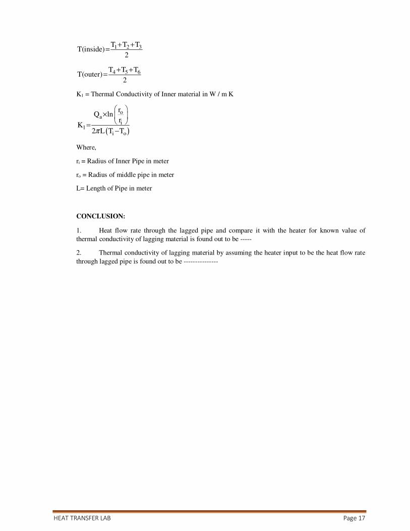
1 2 3T T TT(inside)
2
+ +=
4 5 6T T TT(outer)
2
+ +=
K1 = Thermal Conductivity of Inner material in W / m K
( )
oa
i1
i o
rQ ln
rK
2 L T Tπ
×
=−
Where,
ri = Radius of Inner Pipe in meter
ro = Radius of middle pipe in meter
L= Length of Pipe in meter
CONCLUSION:
1. Heat flow rate through the lagged pipe and compare it with the heater for known value of
thermal conductivity of lagging material is found out to be -----
2. Thermal conductivity of lagging material by assuming the heater input to be the heat flow rate
through lagged pipe is found out to be ---------------

HEAT TRANSFER LAB Page 18
EXPERIMENT – 3
HEAT TRANSFER THROUGH A CONCENTRIC SPHERE
AIM:To find out the thermal conductivity of concentric sphere (Powder)
DESCRIPTION:
The apparatus consists of two thin walled concentric copper spheres. The inner sphere houses the
heating coil. The insulating powder (Asbestos powder – Lagging Material) is packed between the two
shells. The powder supply to the heating coil is by using a dimmerstat and is measured by Voltmeter
and Ammeter. ChoromelAlumel thermocouples are used to measure the temperatures. Thermocouples
(1) to (4) are embedded on inner sphere and (5) to (10) are as shown in the fig. Temperature readings in
turn enable to find out the Thermal Conductivity of the insulating powder as an isotropic material and
the value of Thermal Conductivity can be determined.
Consider the transfer of heat by conduction through the wall of a hollow sphere formed by the
insulating powdered layer packed between two thin copper spheres (Ref. Fig. 1)
Let, ri = radius of inner sphere in meters.
ro = radius of outer sphere in meters.
Ti = average temperature of inner sphere in oC.
To = average temperature of outer sphere in oC.
Where,
1 2i
T TT
2
+= and 3 4
o
T TT
2
+=
Note that T1 to T10 denote the temperature of thermocouples (1) to (10).
From the experimental values of q, Ti and To the unknown thermal conductivity K can be determined as
( )( )
o i
i o i o
q r rK
4 r r T Tπ
−=
× +
SPECIFICATIONS:
1. Radius of the inner copper sphere, ri = 50mm
2. Radius of the outer copper sphere, ro = 100mm
3. Voltmeter (0 – 100 – 200 V).
4. Ammeter (0 – 2 Amps.)
5. Temperature Indicator 0 – 300 0C calibrated for chromelalumel.
6. Dimmerstat 0 – 2A, 0 – 230 V.
HEAT TRANSFER LAB Page 19
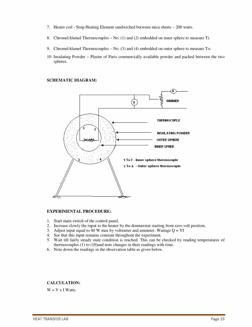
7. Heater coil - Strip Heating Element sandwiched between mica sheets – 200 watts.
8. ChromelAlumel Thermocouples – No. (1) and (2) embedded on inner sphere to measure Ti.
9. ChromelAlumel Thermocouples – No. (3) and (4) embedded on outer sphere to measure To.
10. Insulating Powder – Plaster of Paris commercially available powder and packed between the two spheres.
SCHEMATIC DIAGRAM:
EXPERIMENTAL PROCEDURE: 1. Start main switch of the control panel. 2. Increase slowly the input to the heater by the dimmerstat starting from zero volt position. 3. Adjust input equal to 40 W max by voltmeter and ammeter. Wattage Q = VI 4. See that this input remains constant throughout the experiment. 5. Wait till fairly steady state condition is reached. This can be checked by reading temperatures of
thermocouples (1) to (10)and note changes in their readings with time. 6. Note down the readings in the observation table as given below.
CALCULATION:
W = V x I Watts.

HEAT TRANSFER LAB Page 20
Ti = Inner sphere mean temp. 0C
To = Outer sphere mean temp. 0C
ri = Radius of inner copper sphere = 50 mm. or 0.05m
ro = Radius of outer copper sphere = 100 mm. or 0.1m
Using Equation:
q V I W /m K= × −
( )( )
o i
i o i o
q r rK
4 r r T Tπ
−=
× −
CONCLUSION:
Thermal conductivity of powder is found out to be ____
SPECIMEN CALCULATIONS:
1 2i
T T 142 140T 141
2 2
+ += = =
3 4o
T T 47 49T 48
2 2
+ += = =
( )( )
( )( )
o i
i o i o
q r r 30 0.1 0.05K 0.256 W/m K
4 r r T T 4 3.14 0.05 0.1 141 48π
− −= = =
× − × × × × −
Actual value of gypsum plaster of Paris = 0.22 W/m-K
Thermal Conductivity of Powder
Inner Ball Dia 0.1 m
Outer Ball Dia 0.2 m
S. No. q
(W)
Inner Ball Temperature Outer Ball Temperature ( )
( )o i
i o i o
q r rK
4 r r T Tπ
−=
× −
T1 T2 1 2
i
T TT
2
+= T3 T4
3 4o
T TT
2
+=
EXAMPLE 1 30 142 142 141 47 49 48 0.256
EXAMPLE 2
1
2
HEAT TRANSFER LAB Page 21
EXPERIMENT – 4
THERMAL CONDUCTIVITY OF GIVEN METAL ROD
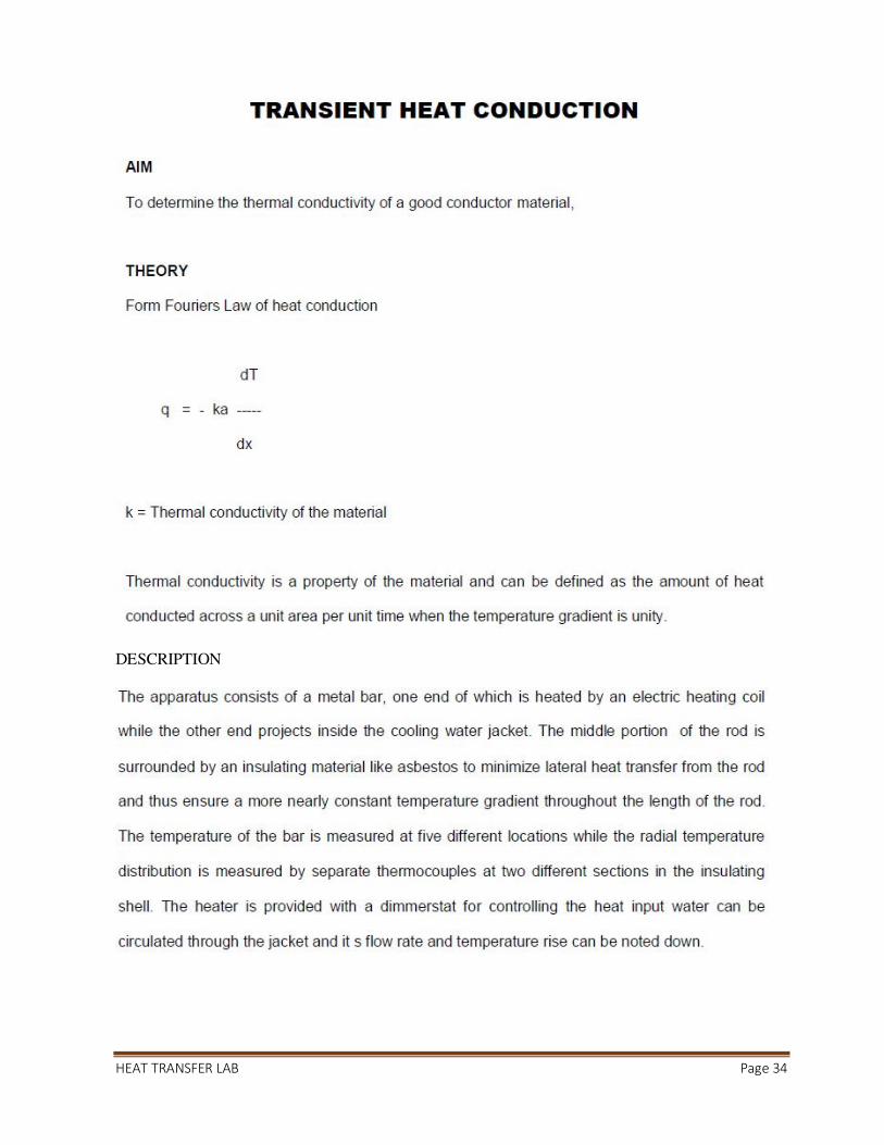
AIM:To determine the thermal conductivity of a good conductor material, say brass.
THEORY:
From Fourier’s law of heat conduction
dTq ka
dx= − , k = thermal conductivity of material.
Thermal conductivity is a property of a material and is defined as the amount of heat conducted across a
unit area per unit time when temperature gradient is unity.
DESCRIPTION:
The apparatus consists of a metal bar, one end of which is heated by an electric heating coil while the
other end projects inside the cooling water jacket. The middle portion of the rod is surrounded by an
insulating material like asbestos to minimize lateral heat transfer from the rod and thus ensure a more
nearly constant temperature gradient throughout the length of the rod. The temperature of the bar is
measured at five different locations while the radial temperature distribution is measured by separate
thermocouples at two different sections in the insulating shell. The heater is provided with a dimmerstat
for controlling the heat input water can be circulated through the jacket and it’s flow rate and
temperature rise can be noted down.
The assumption that at steady state, the heat flow is mainly due to axial conduction can be verified by
the readings of temperature sensors fixed in the insulation material around the rod in radial direction.
Less variation in these readings shall confirm the assumption.
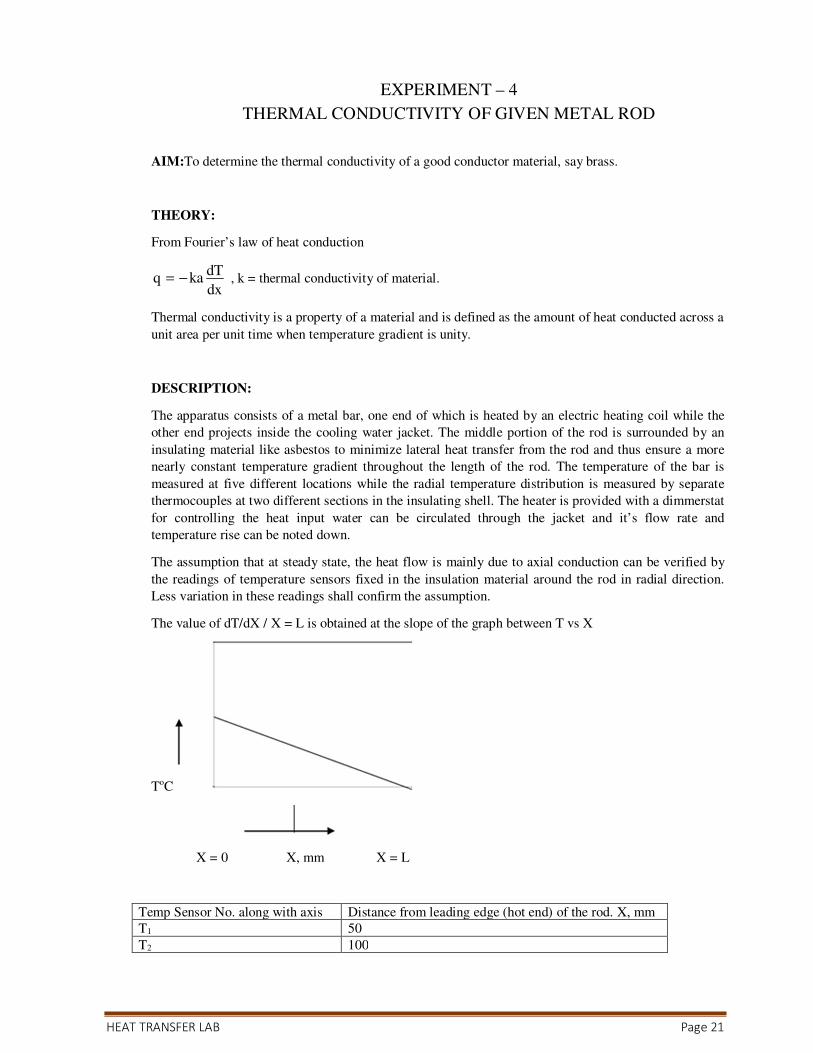
The value of dT/dX / X = L is obtained at the slope of the graph between T vs X
ToC
X = 0 X, mm X = L
Temp Sensor No. along with axis Distance from leading edge (hot end) of the rod. X, mm
T1 50
T2 100

HEAT TRANSFER LAB Page 22
T3 150
T4 200
SCHEMATIC DIAGRAM:
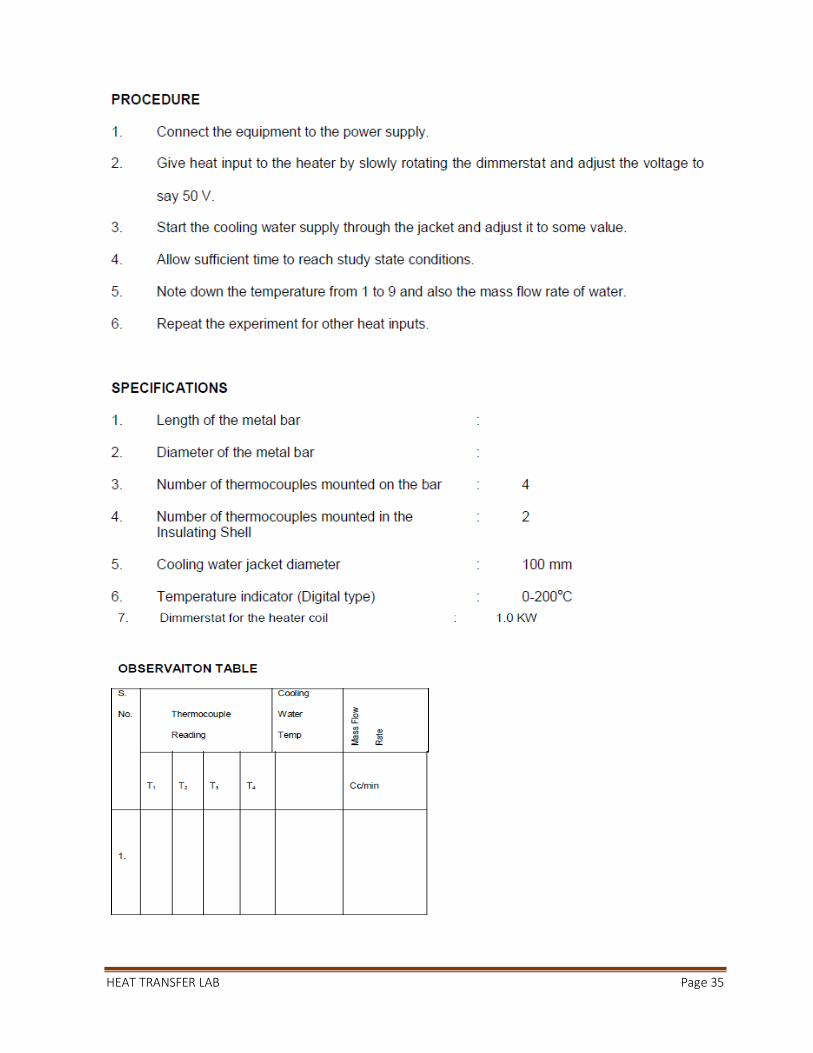
PROCEDURE:
1. Connect the equipment to the power supply.
2. Give heat input to the heater by slowly rotating the dimmerstat and adjust the voltage to say (S25W,
50W etc)
3. Start the cooling water supply through the jacket and adjust it to some value.
4. Allow sufficient time to reach study state conditions.
5. Note down the temperature from 1 to 6 and also the mass flow rate of water.
6. Repeat the experiment for other heat inputs.
7. Repeat the experiment at different heat inputs (Do not exceed 50w).
HEAT TRANSFER LAB Page 23
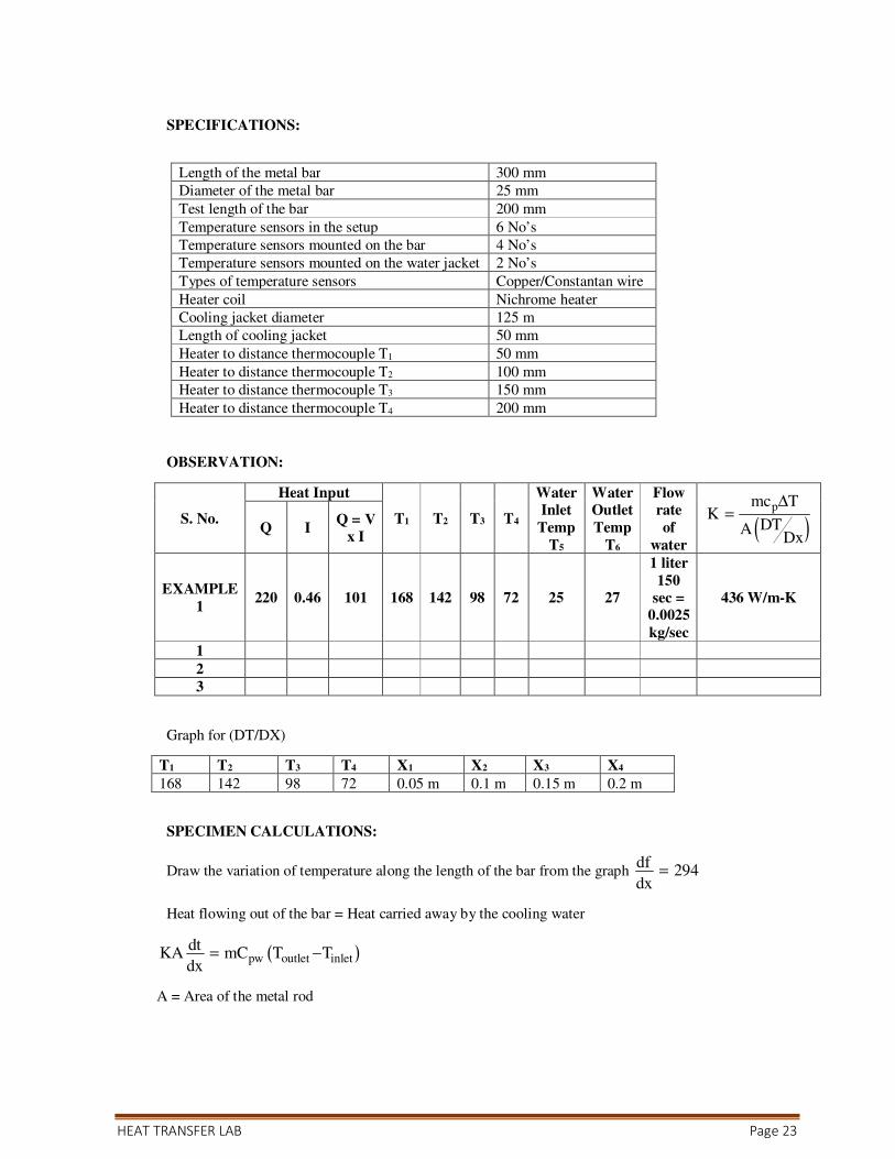
SPECIFICATIONS:
OBSERVATION:
S. No.
Heat Input
T1 T2 T3 T4
Water
Inlet
Temp
T5
Water
Outlet
Temp
T6
Flow
rate
of
water ( )
pmc TK
DTADx
∆=
Q I Q = V
x I
EXAMPLE
1 220 0.46 101 168 142 98 72 25 27
1 liter
150
sec =
0.0025
kg/sec
436 W/m-K
1
2
3
Graph for (DT/DX)
T1 T2 T3 T4 X1 X2 X3 X4
168 142 98 72 0.05 m 0.1 m 0.15 m 0.2 m
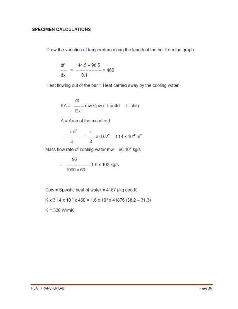
SPECIMEN CALCULATIONS:
Draw the variation of temperature along the length of the bar from the graph df
294dx
=
Heat flowing out of the bar = Heat carried away by the cooling water
( )pw outlet inletdt
KA mC T Tdx
= −
A = Area of the metal rod
Length of the metal bar 300 mm
Diameter of the metal bar 25 mm
Test length of the bar 200 mm
Temperature sensors in the setup 6 No’s
Temperature sensors mounted on the bar 4 No’s
Temperature sensors mounted on the water jacket 2 No’s
Types of temperature sensors Copper/Constantan wire
Heater coil Nichrome heater
Cooling jacket diameter 125 m
Length of cooling jacket 50 mm
Heater to distance thermocouple T1 50 mm
Heater to distance thermocouple T2 100 mm
Heater to distance thermocouple T3 150 mm
Heater to distance thermocouple T4 200 mm
HEAT TRANSFER LAB Page 24
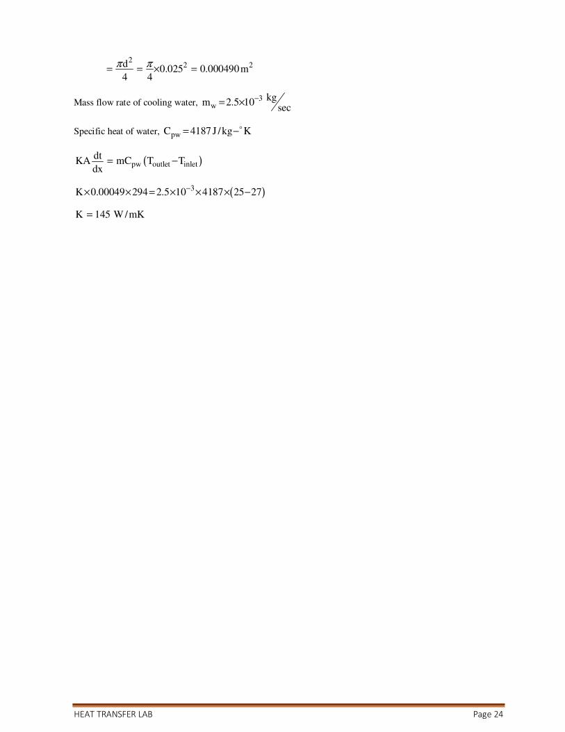
2
2 2d0.025 0.000490m
4 4
π π= = × =
Mass flow rate of cooling water, 3
wkg
m 2.5 10sec
−= ×
Specific heat of water, pwC 4187 J /kg K= −�
( )pw outlet inletdt
KA mC T Tdx
= −
( )3K 0.00049 294 2.5 10 4187 25 27−× × = × × × −
K 145 W /mK=
HEAT TRANSFER LAB Page 25
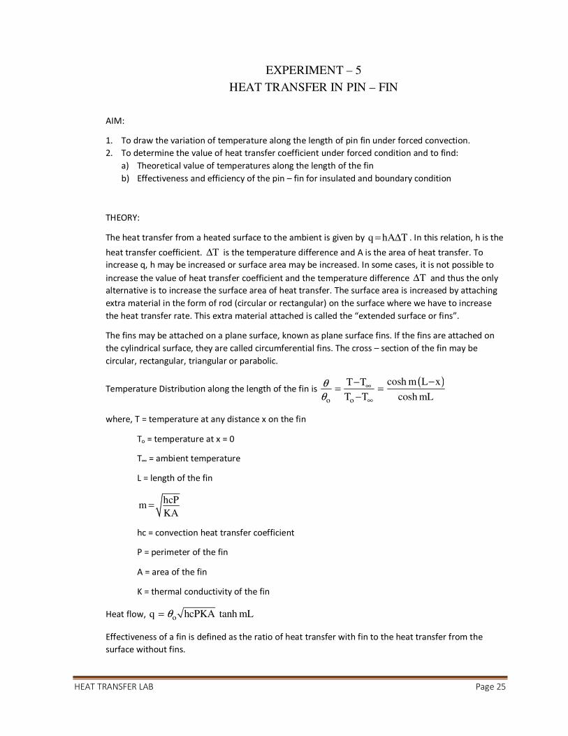
EXPERIMENT – 5
HEAT TRANSFER IN PIN – FIN
AIM:
1. To draw the variation of temperature along the length of pin fin under forced convection.
2. To determine the value of heat transfer coefficient under forced condition and to find:
a) Theoretical value of temperatures along the length of the fin
b) Effectiveness and efficiency of the pin – fin for insulated and boundary condition
THEORY:
The heat transfer from a heated surface to the ambient is given by q hA T= ∆ . In this relation, h is the
heat transfer coefficient. T∆ is the temperature difference and A is the area of heat transfer. To
increase q, h may be increased or surface area may be increased. In some cases, it is not possible to
increase the value of heat transfer coefficient and the temperature difference T∆ and thus the only
alternative is to increase the surface area of heat transfer. The surface area is increased by attaching
extra material in the form of rod (circular or rectangular) on the surface where we have to increase
the heat transfer rate. This extra material attached is called the “extended surface or fins”.
The fins may be attached on a plane surface, known as plane surface fins. If the fins are attached on
the cylindrical surface, they are called circumferential fins. The cross – section of the fin may be
circular, rectangular, triangular or parabolic.
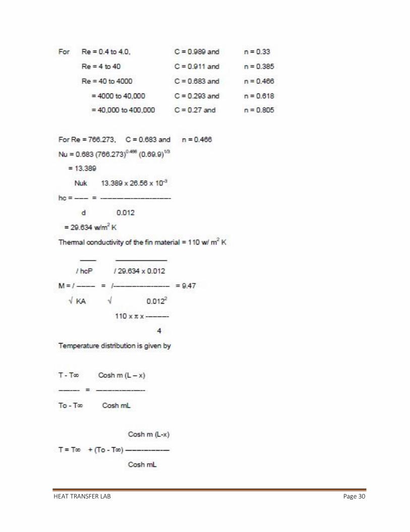
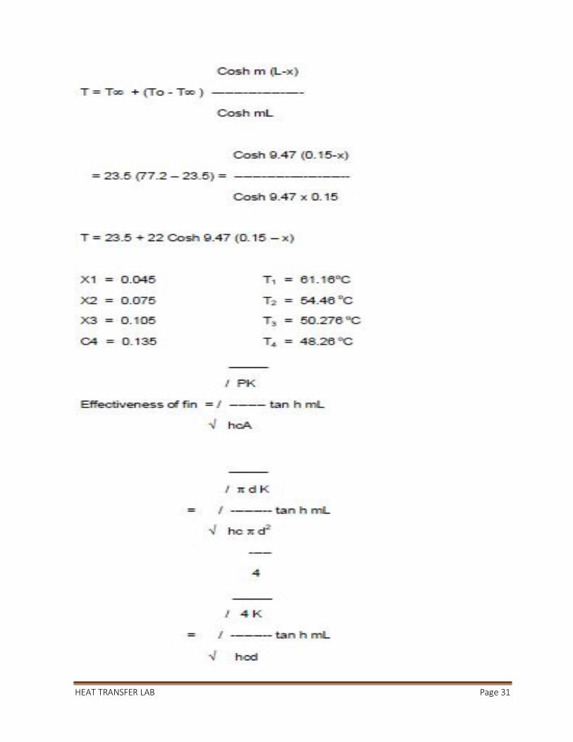
Temperature Distribution along the length of the fin is ( )
o o
cosh m L xT T
T T cosh mL
θθ
∞
∞
−−= =
−
where, T = temperature at any distance x on the fin
To = temperature at x = 0
T∞ = ambient temperature
L = length of the fin
hcP
mKA
=
hc = convection heat transfer coefficient
P = perimeter of the fin
A = area of the fin
K = thermal conductivity of the fin
Heat flow, oq hcPKA tanh mLθ=
Effectiveness of a fin is defined as the ratio of heat transfer with fin to the heat transfer from the
surface without fins.

HEAT TRANSFER LAB Page 26
For end insulated condition
oo
hcPKA tanh mL PKtanh mL
hcA hcAε θ
θ= =
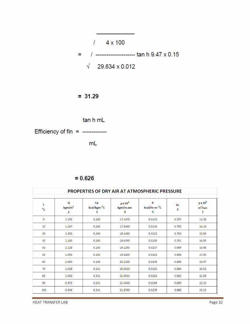
The efficiency of a fin is defined as the ratio of the actual heat transferred by the fin to the maximum
heat transferred by the fin if the entire fin area were at base temperature.
tanh mL
mLη =
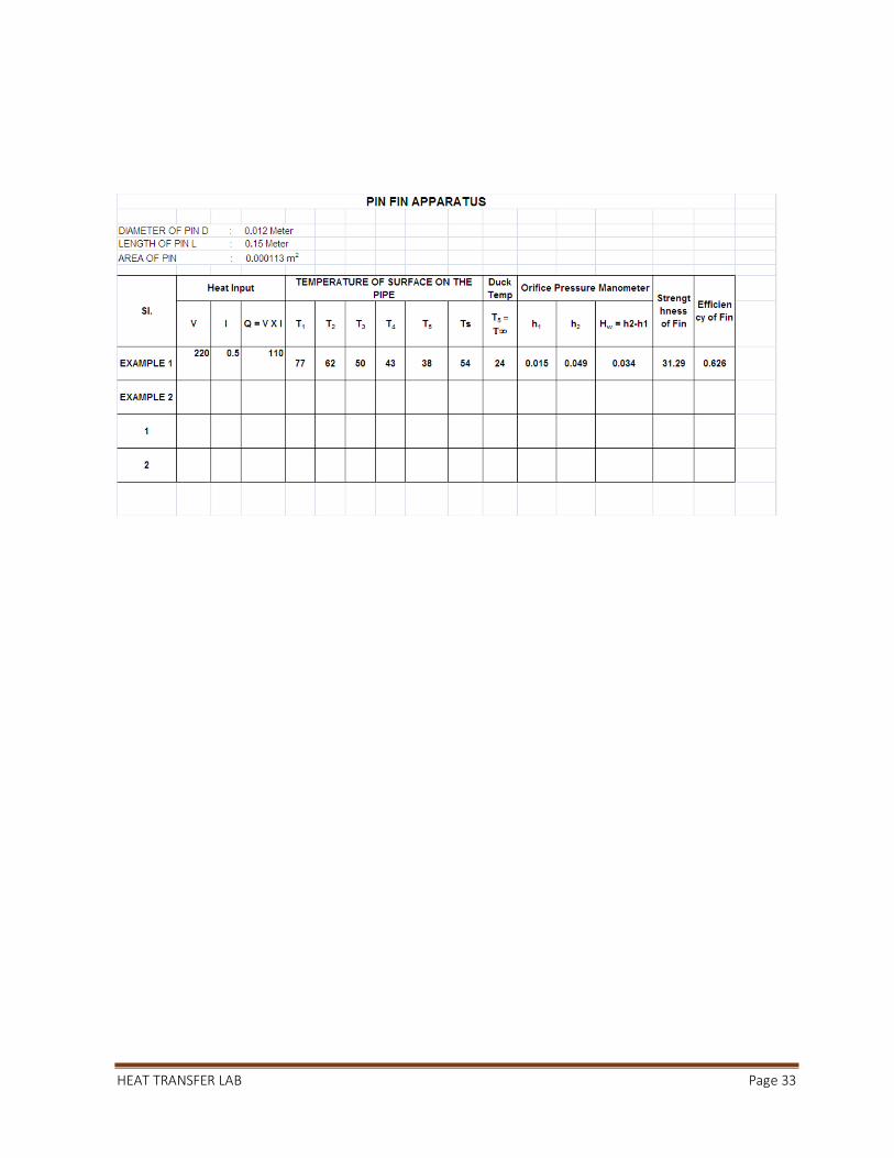
SPECIFICATIONS:
Length of the fin 150 mm
Diameter of the fin 12 mm
Thermal conductivity of fin material (brass) 110 W/m-K
Diameter of the orifice 0.02 m
Duct length 0.5 m
Diameter of the duct 0.15 m
Area of the duct 0.0177 m2
Coefficient of discharge of the orifice 0.68
Density of manometric fluid ( Water) 13.6 x 10³ kg/m3
Type thermocouple Copper/Constantan wire
Heater to Thermocouple T1 distance 25 mm
Heater to Thermocouple T2 distance 50 mm
Heater to Thermocouple T3 distance 75 mm
Heater to Thermocouple T4 distance 100 mm
SCHEMATIC DIAGRAM:

HEAT TRANSFER LAB Page 27
PROCEDURE:
1. Connect the equipment to electric power supply.
2. Keep the thermocouple selector switch to zero position.
3. Turn the dimmerstat knob clockwise and adjust the power input to
the heater to the desired value.
4. Switch on the blower.
5. Set the airf flow rate to any desired value by adjusting the difference in mercury levels in the manometer.
6. Allow the unit to stabilize. 7. Turn the thermocouple selector switch clockwise and note down the
temperature T1 to T6. 8. Note down the difference in level of manometer.
9. Repeat the experiment for different power input to the heater.
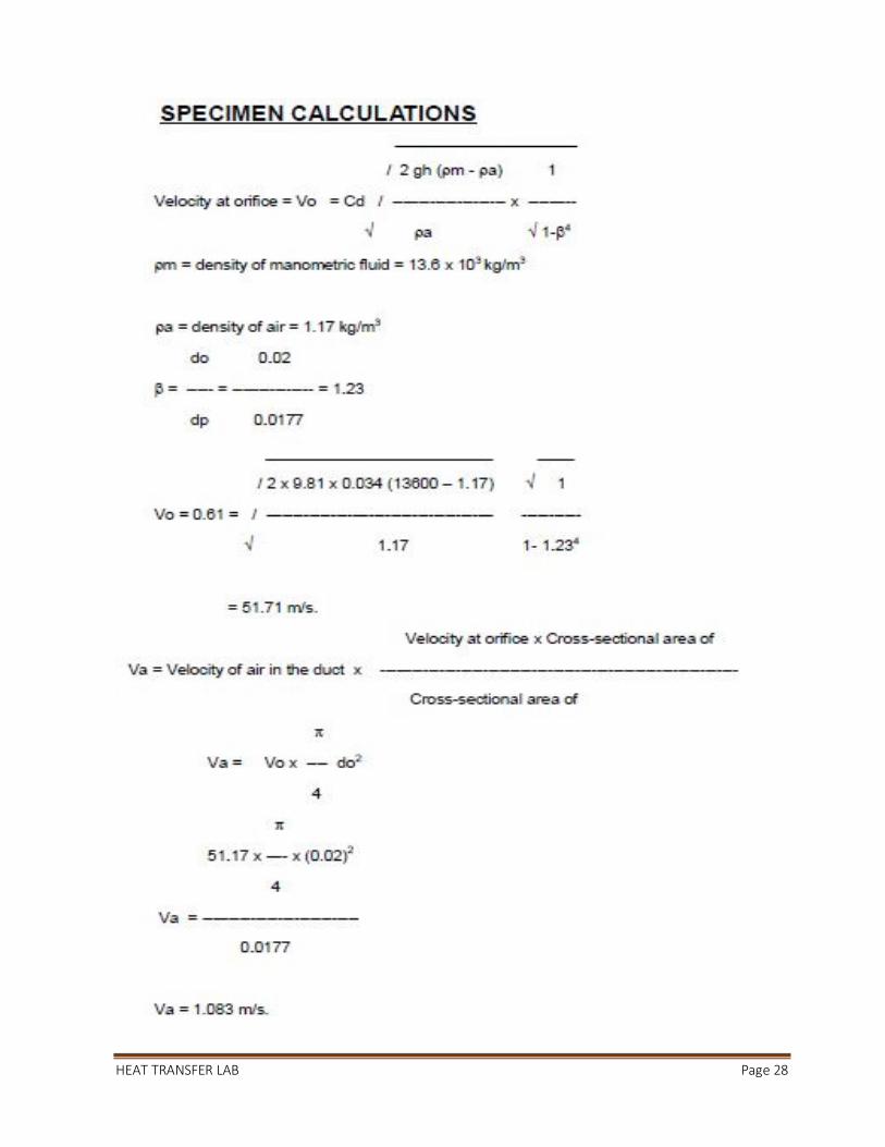
SPECIMEN CALCULATIONS:
Velocity at orifice = ( )m a
o d 4a
2ghV C
1
ρ ρ
ρ β
−=
−
HEAT TRANSFER LAB Page 28

HEAT TRANSFER LAB Page 29
HEAT TRANSFER LAB Page 30
HEAT TRANSFER LAB Page 31
HEAT TRANSFER LAB Page 32
HEAT TRANSFER LAB Page 33
HEAT TRANSFER LAB Page 34
DESCRIPTION
HEAT TRANSFER LAB Page 35
HEAT TRANSFER LAB Page 36
HEAT TRANSFER LAB Page 37

HEAT TRANSFER LAB Page 38
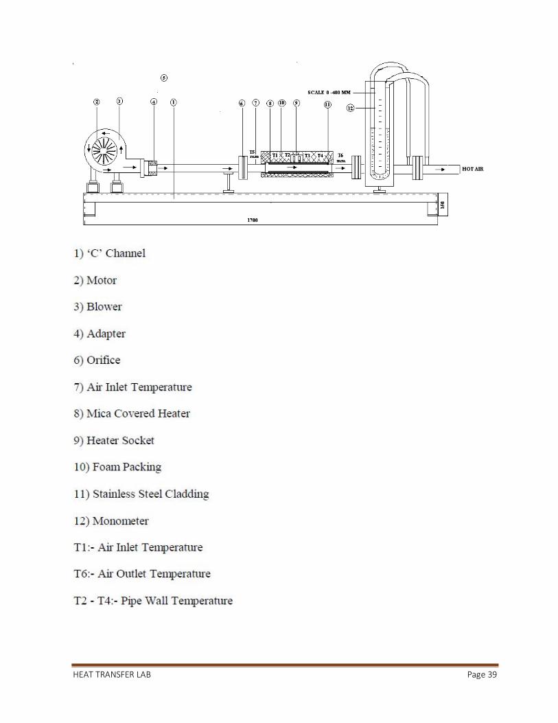
HEAT TRANSFER LAB Page 39

HEAT TRANSFER LAB Page 40

HEAT TRANSFER LAB Page 41
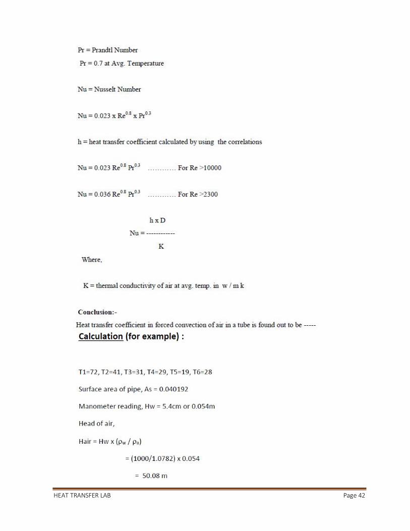
HEAT TRANSFER LAB Page 42
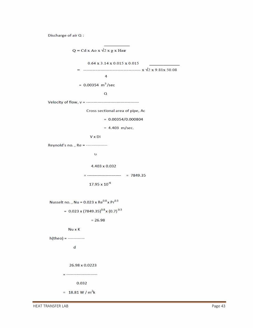
HEAT TRANSFER LAB Page 43

HEAT TRANSFER LAB Page 44

HEAT TRANSFER LAB Page 45

HEAT TRANSFER LAB Page 46
SPECIFICATIONS:

HEAT TRANSFER LAB Page 47
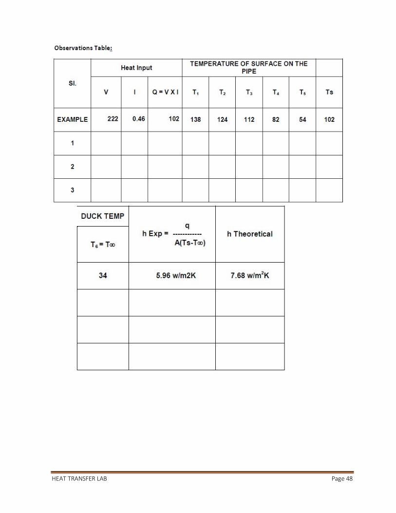
HEAT TRANSFER LAB Page 48

HEAT TRANSFER LAB Page 49

HEAT TRANSFER LAB Page 50
HEAT TRANSFER LAB Page 51
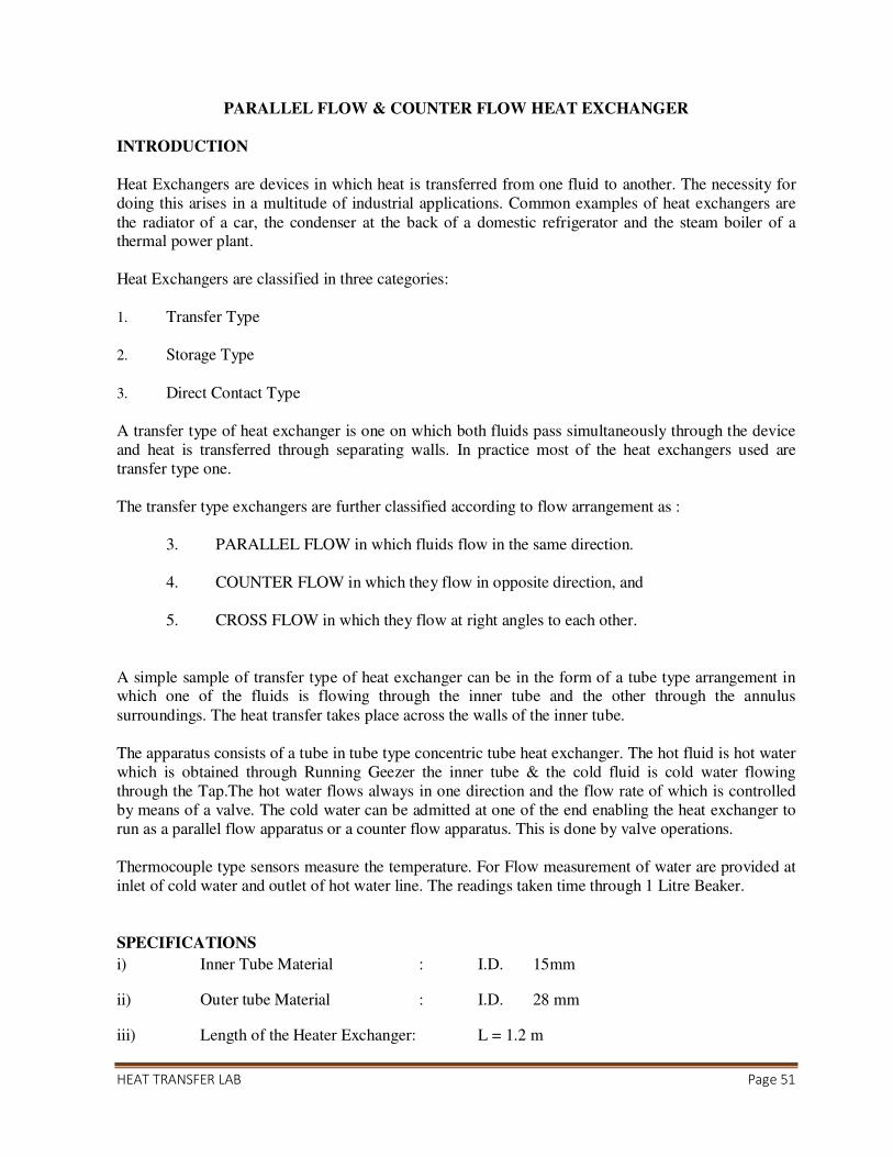
PARALLEL FLOW & COUNTER FLOW HEAT EXCHANGER
INTRODUCTION
Heat Exchangers are devices in which heat is transferred from one fluid to another. The necessity for
doing this arises in a multitude of industrial applications. Common examples of heat exchangers are
the radiator of a car, the condenser at the back of a domestic refrigerator and the steam boiler of a thermal power plant.
Heat Exchangers are classified in three categories:
1. Transfer Type
2. Storage Type
3. Direct Contact Type
A transfer type of heat exchanger is one on which both fluids pass simultaneously through the device
and heat is transferred through separating walls. In practice most of the heat exchangers used are
transfer type one.
The transfer type exchangers are further classified according to flow arrangement as :
3. PARALLEL FLOW in which fluids flow in the same direction.
4. COUNTER FLOW in which they flow in opposite direction, and
5. CROSS FLOW in which they flow at right angles to each other.
A simple sample of transfer type of heat exchanger can be in the form of a tube type arrangement in which one of the fluids is flowing through the inner tube and the other through the annulus
surroundings. The heat transfer takes place across the walls of the inner tube.
The apparatus consists of a tube in tube type concentric tube heat exchanger. The hot fluid is hot water
which is obtained through Running Geezer the inner tube & the cold fluid is cold water flowing
through the Tap.The hot water flows always in one direction and the flow rate of which is controlled
by means of a valve. The cold water can be admitted at one of the end enabling the heat exchanger to
run as a parallel flow apparatus or a counter flow apparatus. This is done by valve operations.
Thermocouple type sensors measure the temperature. For Flow measurement of water are provided at
inlet of cold water and outlet of hot water line. The readings taken time through 1 Litre Beaker.
SPECIFICATIONS
i) Inner Tube Material : I.D. 15mm
ii) Outer tube Material : I.D. 28 mm
iii) Length of the Heater Exchanger: L = 1.2 m

HEAT TRANSFER LAB Page 52
iv) Temperature Controller : Digital 0-200oC
v) Temperature Indicator : Digital 0-199.9oC and least count
0.1oC with multichannel switch.
vi) Temperature Sensors : Thermocouple (5 Nos.)
EXERIMENTAL PROCEDURE
1. Put water in bath and switch on the heaters.
2. Adjust the required temperature of hot water using DTC.
3. Adjust the valve. Allow hot water to recycle in bath through by-pass by switching on the
Geezer.
4. Start the flow through annulus and run the exchanger either as parallel flow unit.
5. Adjust the flow rate on cold water side taken time through 1 Liter Biker.
6. Adjust the flow rate on hot water side taken time through 1 Liter Biker.
7. Keeping the flow rates same, wait till the steady state conditions are reached.
8. Taken the temperature on hot water and cold water side and also the flow rates accurately.
9. Repeat the experiment with a counter flow under identified flow conditions.

HEAT TRANSFER LAB Page 53
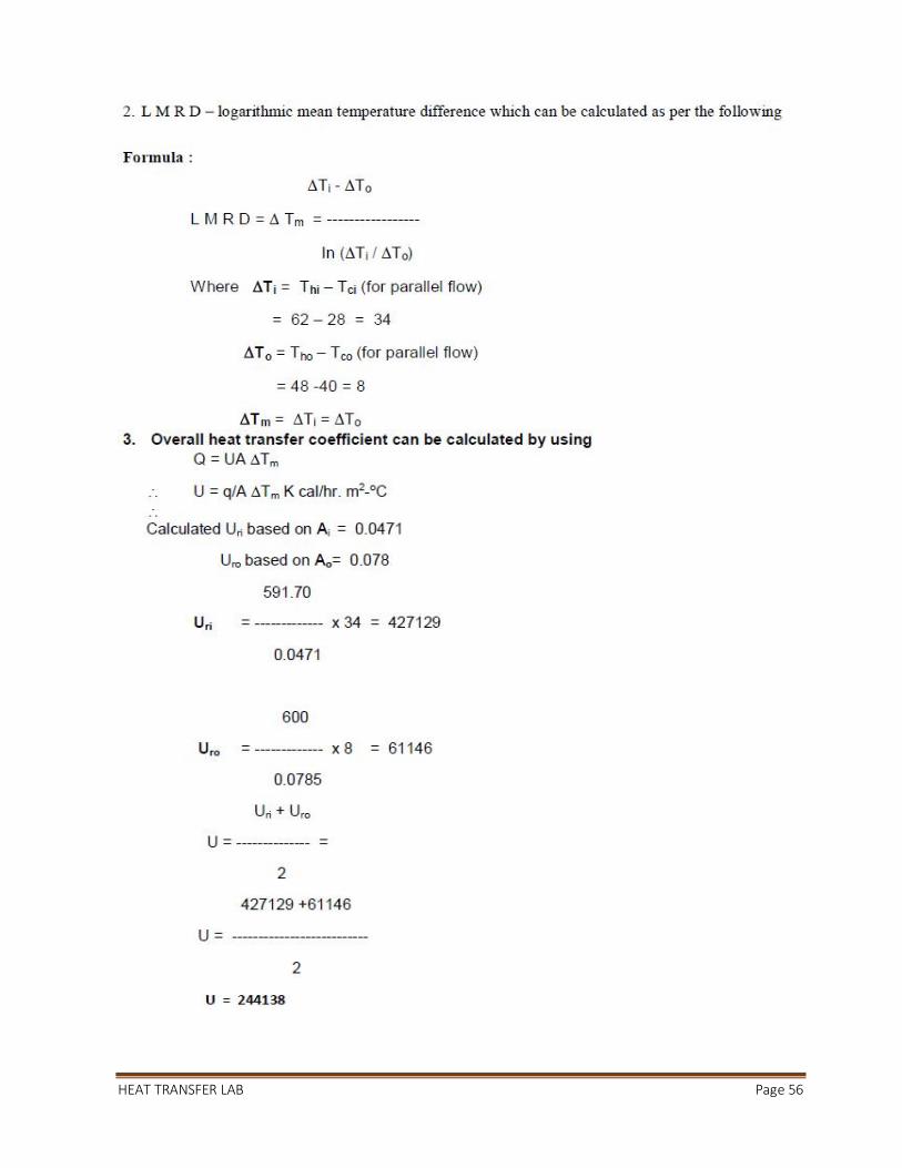
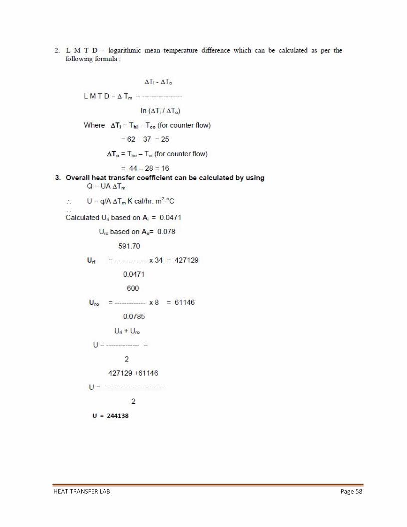
Note that in a special case of Counter Flow Exchanger exists when the heatcapacity rates Cc & Ch are
equal, then Thi – Tco = Tho – Tci thereby making DTi =
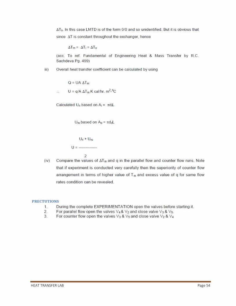
HEAT TRANSFER LAB Page 54

HEAT TRANSFER LAB Page 55
HEAT TRANSFER LAB Page 56

HEAT TRANSFER LAB Page 57
HEAT TRANSFER LAB Page 58

HEAT TRANSFER LAB Page 59
HEAT TRANSFER LAB Page 60
EXPERIMENT – 10
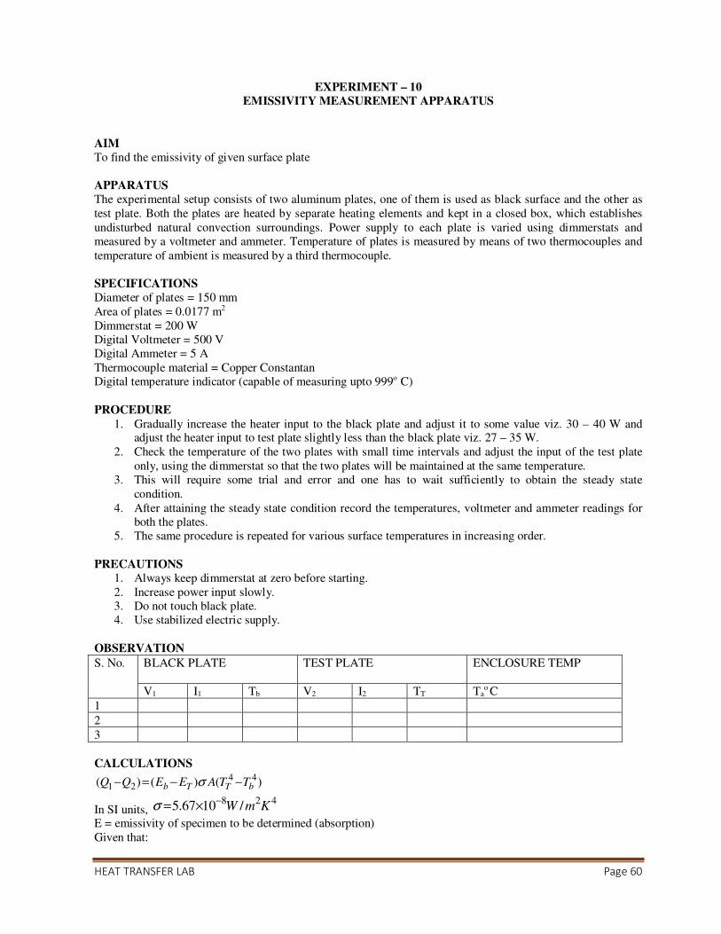
EMISSIVITY MEASUREMENT APPARATUS
AIM
To find the emissivity of given surface plate
APPARATUS
The experimental setup consists of two aluminum plates, one of them is used as black surface and the other as
test plate. Both the plates are heated by separate heating elements and kept in a closed box, which establishes
undisturbed natural convection surroundings. Power supply to each plate is varied using dimmerstats and
measured by a voltmeter and ammeter. Temperature of plates is measured by means of two thermocouples and
temperature of ambient is measured by a third thermocouple.
SPECIFICATIONS
Diameter of plates = 150 mm
Area of plates = 0.0177 m2
Dimmerstat = 200 W
Digital Voltmeter = 500 V
Digital Ammeter = 5 A
Thermocouple material = Copper Constantan
Digital temperature indicator (capable of measuring upto 999o C)
PROCEDURE
1. Gradually increase the heater input to the black plate and adjust it to some value viz. 30 – 40 W and adjust the heater input to test plate slightly less than the black plate viz. 27 – 35 W.
2. Check the temperature of the two plates with small time intervals and adjust the input of the test plate
only, using the dimmerstat so that the two plates will be maintained at the same temperature.
3. This will require some trial and error and one has to wait sufficiently to obtain the steady state
condition.
4. After attaining the steady state condition record the temperatures, voltmeter and ammeter readings for
both the plates.
5. The same procedure is repeated for various surface temperatures in increasing order.
PRECAUTIONS
1. Always keep dimmerstat at zero before starting.
2. Increase power input slowly.
3. Do not touch black plate.
4. Use stabilized electric supply.
OBSERVATION
S. No. BLACK PLATE TEST PLATE ENCLOSURE TEMP
V1 I1 Tb V2 I2 TT Tao C
1
2
3
CALCULATIONS 4 4
1 2( ) ( ) ( )b T T bQ Q E E A T Tσ− = − −
In SI units, 8 2 45.67 10 /W m Kσ −= ×
E = emissivity of specimen to be determined (absorption)
Given that:

HEAT TRANSFER LAB Page 61
Q1 = black plate = 40 W
Q2 = test plate = 38 W
Test plate temp. ( ) 143 273 416TT C K= + =�
Surrounding temp. ( ) 40 273 313sT C K= + =�
4 4
1 2( ) ( ) ( )b T T bQ Q E E A T Tσ− = − −
8 4 4(40 38) (1 ) 5.67 10 0.0154 (416 313 )TE −− = − × × × × −
2 (1 ) 17.76TE= − ×
0.88TE =
RESULT
Hence the emissivity of the test plate is determined.

HEAT TRANSFER LAB Page 62
Experiment – 11
Stefan Boltzmann Apparatus

HEAT TRANSFER LAB Page 63
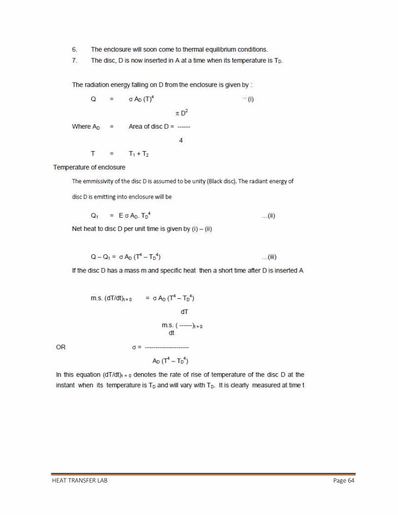
HEAT TRANSFER LAB Page 64

HEAT TRANSFER LAB Page 65
HEAT TRANSFER LAB Page 66
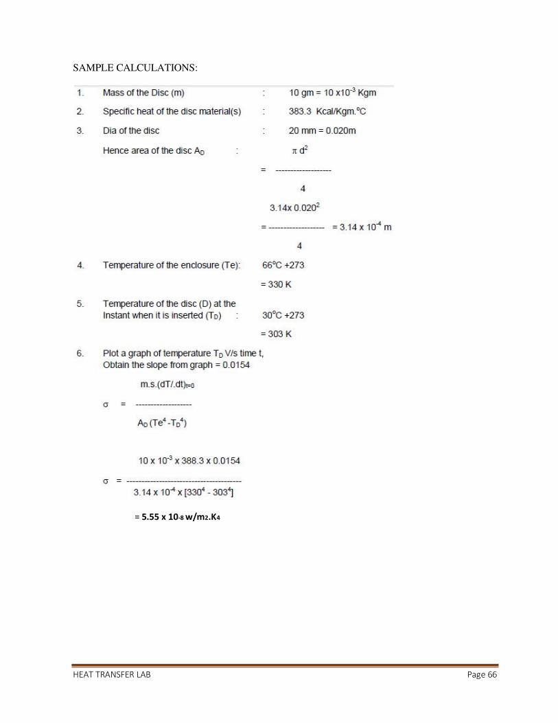
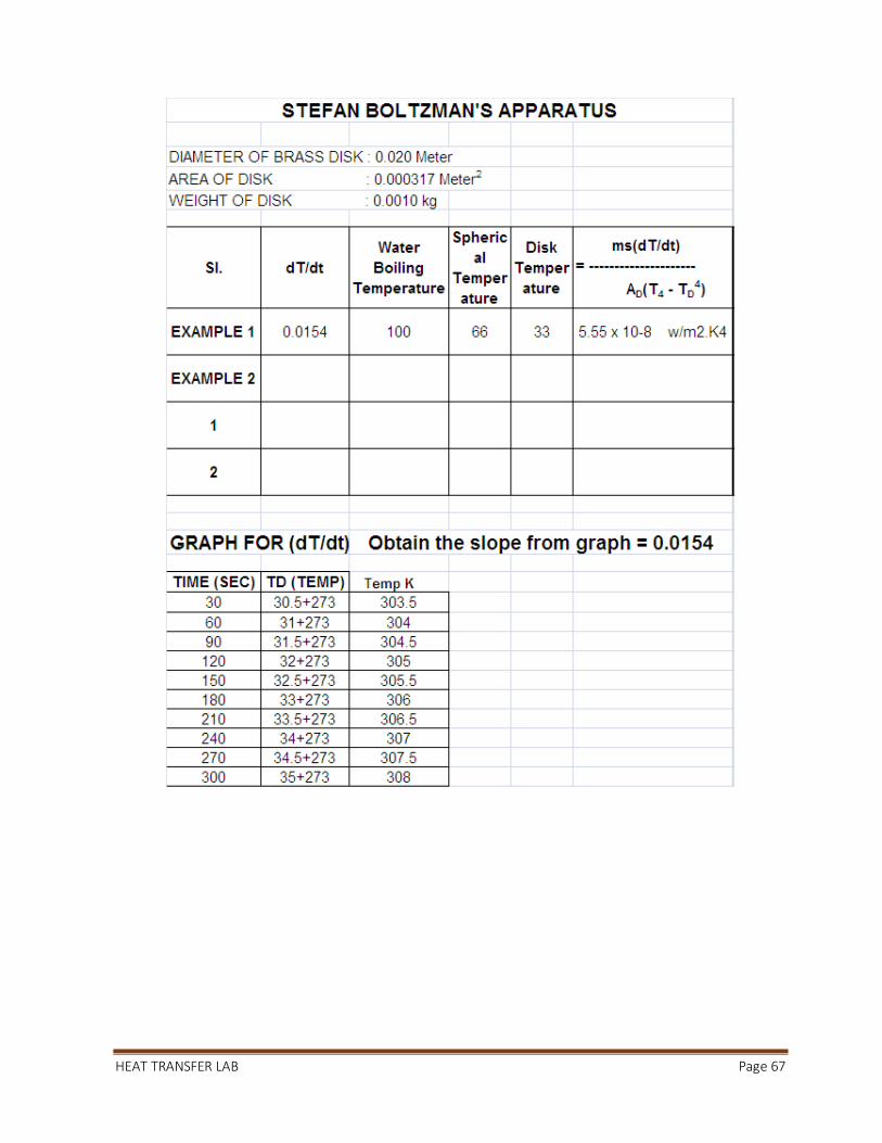
SAMPLE CALCULATIONS:
= 5.55 x 10⁻⁸ w/m2.K4
HEAT TRANSFER LAB Page 67
HEAT TRANSFER LAB Page 68
Experiment – 12
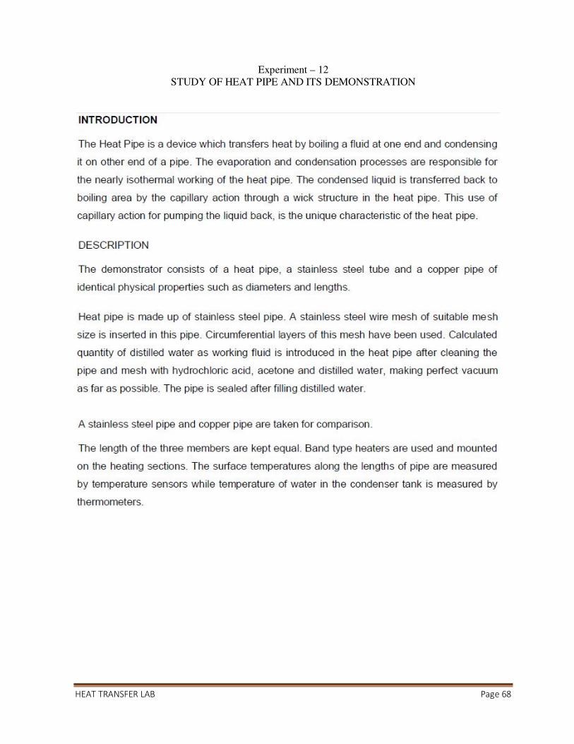
STUDY OF HEAT PIPE AND ITS DEMONSTRATION

HEAT TRANSFER LAB Page 69
HEAT TRANSFER LAB Page 70

HEAT TRANSFER LAB Page 71
Experiment – 13
FILM AND DROPWISE CONDENSATION APPARATUS
AIM: To determine dryness friction of steam by drop wise and film wise condensation.
DESCRIPTION:
SPECIFICATIONS:
PROCEDURE:

HEAT TRANSFER LAB Page 72
CALCULATIONS:
The total heat before dropwise condensation = The total heat after dropwise condensation.
p1 + x = p2 + Cp (t1 – t2)
x = p2 + Cp (t1 – t2) - p1
EXAMPLE:
x = p2 + Cp (t1 – t2) - p1
p1 = 1.241
p2 = 2.5
Cp = 0.24
t1 = 88

HEAT TRANSFER LAB Page 73
t2 = 68
x = 1.241 + 0.24 (88 – 68) - 2.5
x = 3.54

HEAT TRANSFER LAB Page 74
Experiment – 14
CRITICAL HEAT FLUX
AIM: To visualize the pool boiling over the heater wire in different regions upto the critical heat flux point at
which the wire melts.
INTRODUCTION:
When heat is added to a liquid from a submerged solid surface, which is at a temperature higher than the
temperature of the liquid, it is usual for a part of the liquid to change phase. This change of phase is called
boiling.
Boiling is of various types, the type depends upon the temperature difference of the surface and the liquid. The
different types are indicated in which a typical experimental boiling curve obtained in a saturated pool of liquid
is down.
DESCRIPTION:
The apparatus consists of a cylindrical glass container housing and test heater (Nichrome wire). Test heater is
connected also to mains via a dimmer. An ammeter is connected in series while a voltmeter across it to the read
the current and voltage. The glass container is kept on a stand, which is fixed on a metallic platform. There is
provision of illuminating the test heater wire with the help of a lamp projecting light from back and the heater
wire can be viewed through a lens.
This experimental setup is designed to study the pool – boiling phenomenon upto critical heat flux point. The pool boiling over the heater wire can be visualized in the different regions upto the critical heat flux point at
which the wire melts. The heat flux from the wire is slowly increased by gradually increasing the applied
voltage across the test wire and the change over from natural convection to nucleate boiling can be seen.
The formation of bubbles and their growth in size and number can be visualized followed by the vigorous
bubble formation and their immediate carrying over to surface and ending this in the braking of wire indicating
the occurrence of critical heat flux point.
SPECIFICATION:
• Glass container : Dia 150 mm & Height 200 mm
• Nichrome wire size : 0.135 F mm
• Dimmer stat : 10 Amp, 230 volts
• Voltmeter : 0 to 250 V
• Ammeter : 0 to 10 AMP
• Thermometer : 0 to 100o
• Nichrome wire resistance : 6.4 ohms
HEAT TRANSFER LAB Page 75
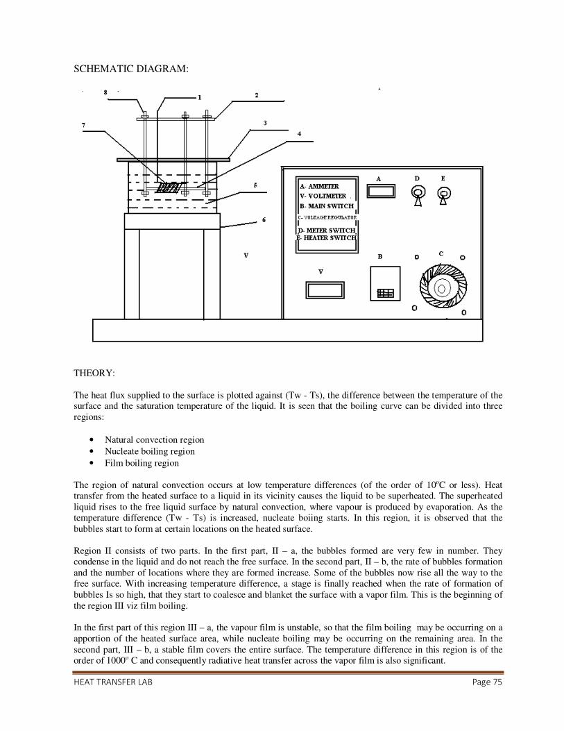
SCHEMATIC DIAGRAM:
THEORY:
The heat flux supplied to the surface is plotted against (Tw - Ts), the difference between the temperature of the surface and the saturation temperature of the liquid. It is seen that the boiling curve can be divided into three
regions:
• Natural convection region
• Nucleate boiling region
• Film boiling region
The region of natural convection occurs at low temperature differences (of the order of 10oC or less). Heat
transfer from the heated surface to a liquid in its vicinity causes the liquid to be superheated. The superheated
liquid rises to the free liquid surface by natural convection, where vapour is produced by evaporation. As the
temperature difference (Tw - Ts) is increased, nucleate boiing starts. In this region, it is observed that the
bubbles start to form at certain locations on the heated surface.
Region II consists of two parts. In the first part, II – a, the bubbles formed are very few in number. They
condense in the liquid and do not reach the free surface. In the second part, II – b, the rate of bubbles formation
and the number of locations where they are formed increase. Some of the bubbles now rise all the way to the
free surface. With increasing temperature difference, a stage is finally reached when the rate of formation of
bubbles Is so high, that they start to coalesce and blanket the surface with a vapor film. This is the beginning of
the region III viz film boiling.
In the first part of this region III – a, the vapour film is unstable, so that the film boiling may be occurring on a
apportion of the heated surface area, while nucleate boiling may be occurring on the remaining area. In the
second part, III – b, a stable film covers the entire surface. The temperature difference in this region is of the
order of 1000o C and consequently radiative heat transfer across the vapor film is also significant.

HEAT TRANSFER LAB Page 76
It will be observed that the heat flux does not increase in a regular manner with the temperature difference. In
region I, the heat flux is proportional to (Tw - Ts)n, where ‘n’ is slightly greater than unity. When the transition
from natural convection to nucleate boiling occurs the heat flux starts to increase more rapidly with temperature
difference, the value of n increasing to about 3. At the end of region II, the boiling curve reaches a peak.
Beyond this, in the region II – A, inspite of increasing temperature difference, the heat flow increases with the
formation of a vapor film. The heat flux passes through a minimum at the end of region III – a. it starts to
increase again with(Tw - Ts) only when stable film boiling begins and radiation becomes increasingly
important.
It is of interest to note how the temperature of the heating surface changes as the heat flux is steadily increased
from zero. Upto point A, natural convection boiling and nucleate boiling occur and the temperature of the
heating surface is obtained by reading off the value of (Tw - Ts) from the boiling curve and adding to it the
value of Ts.
If the heat flux is increased even a little beyond the value of A, the temperature of the surface will shoot up to
the value corresponding to the point C. It is apparent from figure 1 that surface temperature corresponding to
point C is high.
For most surfaces, it is high enough to cause the material to melt. Thus in most practical situations, it is
undesirable to exceed the value of heat flux corresponding to point A. This value is therefore of considerable
engineering significance and is called the critical or peak heat flux. The pool boiling curve as described above is
known as Nukiyam pool boiling curve. The discussions so far has been concerned with the various type of
boiling which occur in saturated pool boiling. If the liquid is below the saturation temperature we say that sub-
cooled pool boiling is taking place. Also in many practical situations, e.g. steam generators; one is interested in boiling in a liquid flowing through tubes. This is called forced convection boiling, may also be saturated or sub
– cooled and of the nucleate or film type.
Thus in order to completely specify boiling occurring in any process, one must state
Whether it is forced convection boiling or pool boiling,
Whether the liquid is saturated or sub – cooled, and
Whether it is in the natural convection nucleate or film boiling region.
PROCEDURE:
• Fill the tank with water.
• Dip the nichrome wire into the water and make the electrical connections.
• Note the current reading in steps of 1 Amp till a maximum current of 10 Amp.
• Between each reading the time interval of two min is allowed for steady state to establish.
• Water temperature is noted with a thermometer at the beginning and at the end of the experiment. The
average of these two is taken as the bulk liquid average temperature.
OBSERVATIONS:
d = Diameter of test wire = 0.135 x 10⁻³ m
L = Length of the test heater = 0.088 m
A = Surface area = PdL = 3.7322 x 10⁻⁵ m2
HEAT TRANSFER LAB Page 77
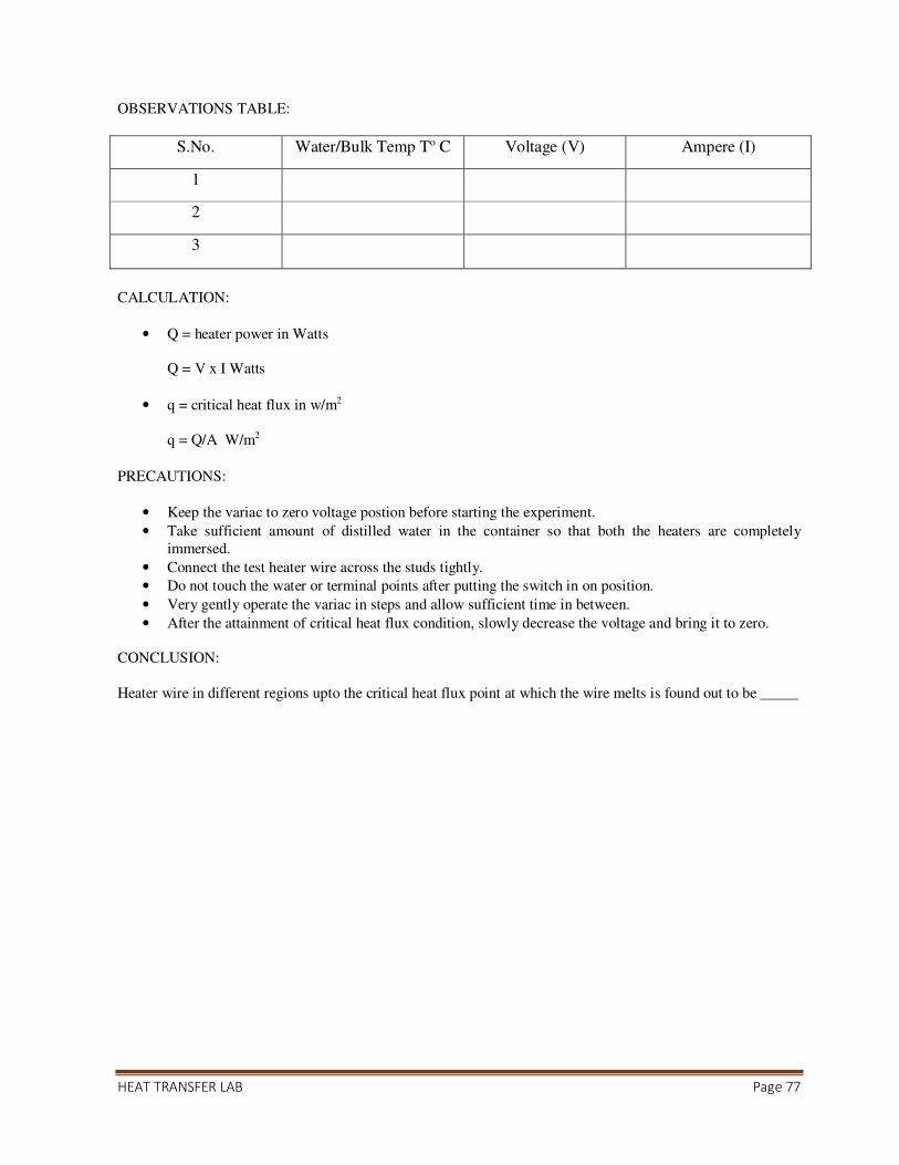
OBSERVATIONS TABLE:
S.No. Water/Bulk Temp To C Voltage (V) Ampere (I)
1
2
3
CALCULATION:
• Q = heater power in Watts
Q = V x I Watts
• q = critical heat flux in w/m2
q = Q/A W/m2 PRECAUTIONS:
• Keep the variac to zero voltage postion before starting the experiment.
• Take sufficient amount of distilled water in the container so that both the heaters are completely
immersed.
• Connect the test heater wire across the studs tightly.
• Do not touch the water or terminal points after putting the switch in on position.
• Very gently operate the variac in steps and allow sufficient time in between.
• After the attainment of critical heat flux condition, slowly decrease the voltage and bring it to zero.
CONCLUSION:
Heater wire in different regions upto the critical heat flux point at which the wire melts is found out to be _____