Landslides and Engineered Slopes – Chen et al. (eds)© 2008 Taylor & Francis Group, London, ISBN 978-0-415-41196-7

Landslides: Seeing the ground

Norbert R. Morgenstern & C. Derek MartinDept. Civil & Environmental Engineering, University of Alberta, Edmonton, Canada

ABSTRACT: Landslide engineering requires the consideration of a number of complex processes ranging fromgeological and hydrogeological characterization to geomechanical characterization, analyses and risk manage-ment. This paper concentrates on recent advances that improve site characterization applied to landslide problems.It presents the view that one of the most exciting developments is the growing potential for application of Geo-graphical Information Systems (GIS) and that making GIS goetechnically smart is a transformative development.Examples are given of integrating remote sensing data in GIS to improve visualization, mapping and movementcharacterization. Application of analysis of rockfall within GIS and complex slope stability evaluation with theaid of GIS are presented to illustrate recent developments and provide direction for future enhancements.

1 INTRODUCTION

A landslide, whether it occurs in a natural or an engi-neered slope, is a complex process. When LauritsBjerrum, at the end of his Terzaghi Lecture (Bjerrrum,1967), reminded us of the recognition in Japan of ‘‘alandslide devil who seems to laugh at human incom-petence’’, he was reminding us of the complexity ofthe landslide process.

Managing complexity invariably requires simpli-fication into a Process Model. A Process Modelcaptures the essentials required to meet the objec-tives of using the model, without including detailsthat are extraneous to these objectives. In geotechnicalengineering these objectives can range from ensuringthat an engineered structure will perform as intendedto managing the risk associated with natural hazardsover a larger scale. Establishing the appropriate pro-cess is both site and project dependent. It underpinsthe value associated with the practice of geotechnicalengineering.

Understanding the landslide process and being ableto simplify it effectively calls on interpreting a numberof contributory processes and activities. The main onesare as follows:

• geomorphology—the multiplicity of physical andchemical processes that have affected the surfaceand near-surface of the site

• hydrology—the role of surface water in infiltration,erosion, etc.

• geology—the sequence and characteristics of thesoils and rocks

• hydrogeology—the factors affecting the groundwa-ter distribution

• geotechnical site characterization• the geotechnical model, seepage, stability and

deformation analyses• risk assessment and risk mitigation

There has been very substantial progress in all ofthese areas in recent years. New tools are applied to sitecharacterization. The range of geomechanical mod-els that can be usefully applied in practice has grownsubstantially. The capacity to analyse often exceedsthe capacity to characterize. Risk assessment andmanagement of slopes is maturing quickly as a valu-able tool for dealing with landslides both locally andregionally. Yet much uncertainty persists in geotech-nical practice. The intrinsic presence of uncertaintyin geotechnical practice was emphasized by Morgen-stern (2000) who provided numerous examples ofunanticipated behaviour of geotechnically engineeredfacilities, often with unfavourable results.

In developing the theme for this paper, we havedrawn on our experience to conclude that the great-est uncertainties in the process modeling of landslidesarise from inadequacies in site characterization, inthe broadest sense, and therefore we concentrate on adiscussion of recent advances that improve site chara-cterization applied to landslide problems.

2 VIEWING THE GROUND SURFACE

2.1 Geographical Information Systems (GIS)

It is our view that one of the most exciting devel-opments for landslide engineering is the growingpotential for application of GIS. The power of GISis that it enables us to ask questions of a database,

3

perform spatial operations on databases and generategraphic output that would be laborious or impossibleto do manually. Rhind (1992) observes that a GIS cananswer five generic questions:

Question Type of Task

1. What is at . . . ..? Inventory2. Where is. . ...? Monitoring3. What has changed since. . .? Inventory and

monitoring4. What spatial pattern exists..? Spatial analysis5. What if. . ...? Modelling

The first three questions are simple queries, while thelast two are more analytical.

GIS on its own adds enormously to our capacityto see and interpret surface geospatial informationwhich is essential for landslide engineering. A firstfly-by experience in GIS soon convinces the landslideengineer of its potential. However, GIS has limita-tions in presenting three-dimensional (3D) geologicand geotechnical data since it was originally devel-oped to deal with two dimensional plane problems.Some GIS systems, like ArcGIS, provide a functionaldeveloper kit which can be used to develop the 3Dcapability for geotechnical engineering problems. Aspointed out by Lan & Martin (2007), the many currentdevelopments in 3D GIS are still not sufficient to meetthe needs of the geotechnical engineer. Mining soft-ware such as Surpac Vision provides a comprehensivesystem for geological modeling, but not geotechni-cal modeling. For example, while three-dimensionalsolid modeling and two-dimensional sections can beeasily created in Surpac, querying inclinometer orpiezometer data is not easily accomplished. Howeveran integrated system, which is illustrated in Figure 1,can be developed.

Even within Stage 1, limited ground behaviour canbe modelled. The aim of Stage 2 is to establish acomprehensive ground model of the site. Stage 3links geotechnical numerical analysis tools to conductgeotechnical analyses and assist in decision-making.Making GIS geotechnically smart is a transformativedevelopment for geotechnical engineering. Examplesto illustrate this will follow in subsequent sections ofthe paper which will return to demonstrate the role ofGIS in a number of slope related problems.

2.2 Aerial and terrestrial photographs

Aerial photographs are a well established resourcefor landslide studies and this is well-understood(Soeters & Van Westen 1996). Aerial photographs canbe used for interpretation (API) for qualitative anal-ysis and photogrammetry for extracting quantitativeinformation. The former has been an essential tool for

Figure 1. The architecture for an integrated system. Itis composed of three different stages which required theimplementation of specific tasks.

the landslide engineer for many years, although oftenneglected in many geotechnical curricula. The latterhas usually been the preserve of specialists.

To recognize landslides, API relies on characteristicmorphology, vegetation and drainage. Parise (2003)provides an example of how diagnostic surface fea-tures can be related to certain types of movement, thedegree of activity and the depth of movement. Thestudy of sequential photographs can provide informa-tion on the progressive evolution of landslides andcan lead to a better understanding of their causes(Chandler & Brunsden, 1995; Van Westen & Getahun,2003). GIS facilitates the application of API, thearchiving of the photos and the production of geomor-phological maps that arise from the interpretation.

While the application of API is common, morequantitative studies are rare, probably due to limitedavailability of good quality photographs, adequatelyfixed control points and cost. Modern photogrammet-ric software has been developed that should encouragegreater use of photogrammetry for the constructionof high quality digital elevation models (DEM). Dif-ferential DEMs will quantify landslide movements.

4

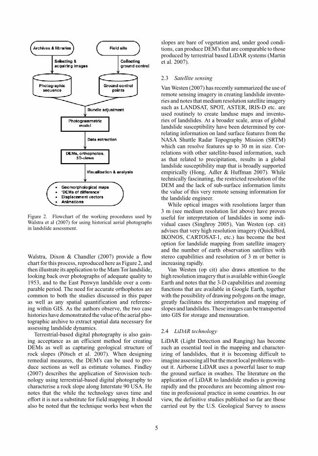
Figure 2. Flowchart of the working procedures used byWalstra et al (2007) for using historical aerial photographsin landslide assessment.

Walstra, Dixon & Chandler (2007) provide a flowchart for this process, reproduced here as Figure 2, andthen illustrate its application to the Mam Tor landslide,looking back over photographs of adequate quality to1953, and to the East Penwyn landslide over a com-parable period. The need for accurate orthophotos arecommon to both the studies discussed in this paperas well as any spatial quantification and referenc-ing within GIS. As the authors observe, the two casehistories have demonstrated the value of the aerial pho-tographic archive to extract spatial data necessary forassessing landslide dynamics.

Terrestrial-based digital photography is also gain-ing acceptance as an efficient method for creatingDEMs as well as capturing geological structure ofrock slopes (Pötsch et al. 2007). When designingremedial measures, the DEM’s can be used to pro-duce sections as well as estimate volumes. Findley(2007) describes the application of Sirovision tech-nology using terrestrial-based digital photography tocharacterise a rock slope along Interstate 90 USA. Henotes that the while the technology saves time andeffort it is not a substitute for field mapping. It shouldalso be noted that the technique works best when the

slopes are bare of vegetation and, under good condi-tions, can produce DEM’s that are comparable to thoseproduced by terrestrial based LiDAR systems (Martinet al. 2007).

2.3 Satellite sensing

Van Westen (2007) has recently summarized the use ofremote sensing imagery in creating landslide invento-ries and notes that medium resolution satellite imagerysuch as LANDSAT, SPOT, ASTER, IRIS-D etc. areused routinely to create landuse maps and invento-ries of landslides. At a broader scale, areas of globallandslide susceptibility have been determined by cor-relating information on land surface features from theNASA Shuttle Radar Topography Mission (SRTM)which can resolve features up to 30 m in size. Cor-relations with other satellite-based information, suchas that related to precipitation, results in a globallandslide susceptibility map that is broadly supportedempirically (Hong, Adler & Huffman 2007). Whiletechnically fascinating, the restricted resolution of theDEM and the lack of sub-surface information limitsthe value of this very remote sensing information forthe landslide engineer.

While optical images with resolutions larger than3 m (see medium resolution list above) have provenuseful for interpretation of landslides in some indi-vidual cases (Singhroy 2005), Van Westen (op. cit)advises that very high resolution imagery (QuickBird,IKONOS, CARTOSAT-1, etc.) has become the bestoption for landslide mapping from satellite imageryand the number of earth observation satellites withstereo capabilities and resolution of 3 m or better isincreasing rapidly.

Van Westen (op cit) also draws attention to thehigh resolution imagery that is available within GoogleEarth and notes that the 3-D capabilities and zoomingfunctions that are available in Google Earth, togetherwith the possibility of drawing polygons on the image,greatly facilitates the interpretation and mapping ofslopes and landslides. These images can be transportedinto GIS for storage and mensuration.

2.4 LiDAR technology

LiDAR (Light Detection and Ranging) has becomesuch an essential tool in the mapping and character-izing of landslides, that it is becoming difficult toimagine assessing all but the most local problems with-out it. Airborne LiDAR uses a powerful laser to mapthe ground surface in swathes. The literature on theapplication of LiDAR to landslide studies is growingrapidly and the procedures are becoming almost rou-tine in professional practice in some countries. In ourview, the definitive studies published so far are thosecarried out by the U.S. Geological Survey to assess

5

landslide susceptibility in Seattle, Washington (Schulz2004, Schulz 2007).

In this case, airborne laser pulses were uniformlyspaced within a 600 m wide swath with an averagepulse density of 1/m2. Up to four laser returns werecollected for each pulse resulting in a vertical pro-file of ground features for each pulse location. Eachpulse generates multiple returns due to reflectionsfrom features such as powerlines, buildings, trees,undergrowth and the ground surface. Simultaneousacquisitions of aircraft position and laser directionlocated laser returns with absolute vertical and hor-izontal accuracy of 15 cm and less than 1 m, respec-tively (Schulz 2004). Swathes are stitched together intoa seemless DEM during processing.

All ground features that produce returns are repre-sented in the laser survey, including buildings, treesand boulders. One of the most valuable develop-ments is that the trees can be stripped away becausesome pulses penetrate the tree canopy and othersare reflected off the forest floors. The latter can beseparated from reflections from the trees to producebald-earth DEM’s. This processing for deforestationis a remarkable contribution but as pointed out byHaugerud & Harding (2001), there are some limi-tations in the algorithms that need to be recognizedin interpreting the bare-earth DEM’s. The techniquehas even been applied to faulting studies in high-relief Alpine landscapes, with spectacular results(Cunningham et al. 2006).

In the case of the Seattle bare-earth DEM, thevertical accuracy is typically about 30 cm, but is sig-nificantly less in areas of high vegetation. The data inthe DEM have a grid cell size of 1.8 m. This DEMwas entered into a GIS to produce a landslide mapusing derivatives of the DEM such as shaded reliefmaps (hill shades), a slope map, a topographic contourmap and numerous ground surface profiles with a 2 mcontour interval. This was supplemented by historicalinformation and ground mapping.

The strength and weaknesses of LiDAR mappingare discussed in detail by Schulz (2007). It is of inter-est to note his conclusions that aerial photographsappeared to be more effective than LiDAR in theSeattle area for discerning boundaries of recentlyactive landslides within landslide complexes. The res-olution of the LiDAR data appeared inadequate toresolve landslide boundaries within landslide com-plexes. However, LiDAR was much more effectivefor identifying presumably older landslides and theboundaries of complexes in which recently activelandslides occurred. Another recent example illustrat-ing the value of high resolution DEM’s provided byLiDAR for mapping landslides has been provided byArdizzone et al. (2007).

Improvements in LiDAR technology, including pro-cessing, are rapidly leading to even more accurate bare

earth DEM’s. Examples of a bare earth DEM witha 1 m resolution applied to landslide studies and abare-earth DEM with 25–50 cm resolution applied tofaulting studies are citied by Carter et al. (2007).

Airborne LiDAR is increasingly being applied tomap landslides and contribute to infrastructure loca-tions such as pipelines and to develop landslide mapswhich contribute to risk analysis. The ability to pene-trate forest cover, even with reduced DEM accuracy, isof enormous value. The increased accuracy of DEM’sforesees the increasing use of differential LiDAR tomeasure ground deformations with time.

As an illustration of the use of LiDAR in currentpractice, Figure 3 shows the bare earth projectionside by side with conventional aerial photographyof a potential pipeline crossing of a river in centralBritish Columbia. While most crossings are by hor-izontal directional drilling, design for conventionalcrossings by excavation methods are needed as astand-by. Hence landslide identification is an impor-tant consideration in route selection. In this casethe river has downcut into a deep deposit (∼200 m)of glacio-lacustrine clays. The contrast between theinformation revealed by the bare earth imagery andconventional airphotos is striking.

While airborne LiDAR is commonly used for largerscale studies, it is also of value to enhance detailedgeological studies at specific sites. Jaboyedoff et al.(2007) has suggested that the high resolution LiDARDEM can be used to extract both regional and localscale geological structures. The advantages of suchtechniques are obvious when dealing with steep moun-tainous terrain. Figure 4 shows a portion of the famousTurtle Mountain-Frank Slide in Canada and the use ofshading relief of a high resolution LiDAR DEM to por-tray the extent of tension cracks that still exist beyondthe scarp of the slide (Sturznegger et al. 2007). Thepotential instability associated with these cracks is amatter of concern.

Figure 3. Example of a LiDAR bare-earth projection com-pared to the conventional aerial photograph.

6

Figure 4. Structural and tension crack mapping of the FrankSlide using LiDAR DEM.

In addition to airborne LiDAR, terrestrial-basedLiDAR is also finding applications in slope stabilitystudies. Examples of rock slope assessment, whereLiDAR has been used to evaluate rock structure aregiven by Kemeny et al. (2006) & Martin et al. (2007).Using terrestrial based LiDAR portable scanners thatcan operate in the range of 50 m to 800 m greatlyenhance our ability to map the slope discontinuities.Sturzenegger et al. (2007) combined both airborne andterrestrial-based LiDAR to map the structural featuresassociated with Frank Slide (Fig. 4). Terrestrial-basedLiDAR is also being used for direct monitoring of theprocess of hard rock coastal cliff erosion (Rosser et al.2005).

3 GIS AND LANDSLIDE SUSCEPTIBILITY

As stated by Van Westen (op cit), GIS has determined,to a large degree, the current state of the art in landslidehazard and risk assessment, particularly for landslidestudies that cover large areas. Chacón et al. (2006) haverecently conducted a comprehensive general review ofGIS landslide mapping techniques and basic conceptsof landslide mapping. From this extensive investiga-tion they identify three main groups of maps that havebeen propagated by means of GIS:

1. Spatial incidence of landslides2. Spatial-temporal incidence and forecasting of land-

slides (hazard susceptibility)3. Consequence of landslides.

Regional studies might characteristically havescales of 1:50,000 and smaller, while site spe-cific studies will have larger scales ranging from1:1000–1:25,000 depending on the project. At theselarger scales one is characteristically merging from

broader Engineering Geology or Geomorphology toGeotechnical Engineering.

The development of a landslide map, an essentialfor any hazard on risk assessment tool, relies primarilyon the visualization techniques summarized previ-ously. Aerial photo interpretation remains widely usedand is increasingly enhanced by LiDAR imagery. GISand image processing software facilitate the process.Soeters & Van Westen (1996) have summarized thegeomorphic features that are diagnostic of landslidesboth recent and relict.

The assessment of landslide susceptibility goesbeyond the cataloguing of past and current landslidesby including areas that are susceptible to sliding.Ideally a susceptibility assessment is based on fieldreconnaissance to determine factors contributing toinstability, utilizing the landslide inventory as a firststep. Landslide susceptibility maps have been pub-lished for many decades (e.g., Radbruch & Crowther1973). However the ability to manipulate geomor-phic data within GIS has proliferated the number oflandslide susceptibility studies and their associatedmethodology. Even prior to the use of GIS basedtechniques, relative landslide susceptibility in termsof simple bivariate analyses or more complex multi-variate analyses had been developed. Early zonationmethods based on these developments have been dis-cussed by Varnes (1984). More recent GIS-baseddevelopments are listed in Chacón et al (op cit). Somehighlights cited are:

• Franks et al. (1998) prepared detailed 1:1000 the-matic maps in GIS for landslide hazards on HongKong Island, based on a very rich database.

• Wachal & Huduk (2000) used GIS to assess lands-liding in a 1,500–2,000 km2 area in the USA basedon four factors—slope angle, geology, vegetationand distance to faults.

• Dai & Lee (2004) developed probabilistic measuresof landslide susceptibility for Lantau Island usingmultivariate logistic regression of presence-absenceof dependent variables relating landslides and con-tributing factors such as lithology, slope angle, slopeaspect, elevation, soil cover, and distance to streamchannels.

There is a tendency to incorporate increasinglycomplex statistical methods in these landslide suscep-tibility analyses. Spatial validation is essential for anypractical application.

Temporal considerations most commonly enter intolandslide susceptibility forecasting by coupling rain-fall probability assessment as an important triggeringfactor (Lan et al. 2005). This can be undertakenempirically or on a more process-based consideration.The work of Mejia-Navarvo et al (1994) provides anexample of the former while that of Dietrich et al.(1995) is an early example of the latter.

7

The inclusion of geomechanical and hydro-logical process considerations within GIS basedmodeling and landslide hazard analysis marks aconvergence between the techniques for regional-based studies developed by Engineering Geom-orphologists and Geologists and the inputs of theGeotechnical Engineer. Here the example offered byDelmonaco et al. (2003) is of interest. In this casethe infinite slope analysis was applied at a river basinscale with basin scale characterization of all of theinputs to this classical equation. In order to calcu-late the likely pore pressure development, Green-Amptinfiltration analyses were also carried out over thebasin scale, reflecting the variation of rainfall withdifferent return periods. The relation between poten-tial instability and return period was determined andthe predicted scenarios of instability were found tocorrespond sensibly with observations made after anextreme rainfall event in 1966. Examples like thisencourage the integration of process-based consid-erations into GIS-based hazard and risk analyses.The coupling of landslide susceptibility forecasts withearthquake effects have already been investigated in aGIS environment (Refice & Capolongo 2002).

The centrality of GIS-based processing has greatlyadvanced regional landslide hazard and risk analy-sis as summarized by Chacón et al. (2006). Therehas been some convergence between the tools usedin regional studies and those used by geotechnicalengineers in more site specific problems. As statedin Section 2, current GIS technology has signifi-cant limitations in truly three-dimensional problems.Chacón et al. (2006) concluded that ‘‘the use ofthree-dimensional GIS for large scale, detailed haz-ard or risk maps will be one of the significantdevelopments in the near future’’. This, applied tolandslide engineering, is the fundamental theme ofthis paper. Günther et al (2004) illustrate the kindof progress that is being made in their extensionto GIS, designated RSS-GIS, that incorporates thedeterministic evaluation of rock slope stability and isparticularly useful for regional stability assessment.It incorporates grid-based data on rock structures,kinematic analyses for hard rock failure modes, somepore pressure effects and stability evaluations on apixel basis. Other examples of integration of geotech-nical considerations with GIS follow later in this paper,see Section 5, 6 and 7.

4 MAPPING GROUND MOVEMENT

4.1 InSar

Since the late 1990’s the application of spaceborneInterferometric Synthetic Aperture Radar (InSAR) has

slowly been incorporated into geo-engineering prac-tice for mapping the rates and extents of ground defor-mations associated with landslides. As the potentialapplications and limitations of this tool are graduallybeing understood, the range of terrains and situationsto which it may be applied are expanding. The strengthof this technique is that either available archives of datacan be utilized to better understand historical move-ments or new data can be acquired for go-forwardmonitoring for large areas (up to 2500 km2) usinga remote platform that can acquire data at night orthrough clouds.

Synthetic aperture radar (SAR) is an active sen-sor that can be used to measure the distance betweenthe sensor and a point on the earth’s surface.A SAR satellite typically orbits the earth at an alti-tude of approximately 800 km. The satellite constantlyemits electromagnetic radiation to the earth’s sur-face in the form of a sine wave, which reflects offthe earth’s surface and returns back to the satel-lite. The back-scattered microwave signal is used tocreate a SAR satellite image (a black and white rep-resentation of ground reflectivity) using SAR signalprocessing methods. SAR radar images are madeup of pixels, with the specific size influenced bythe SAR sensor resolution; the higher the resolu-tion the smaller the pixel size. To measure dif-ferential ground movements over a specified timeperiod, InSAR requires two SAR images of the samearea taken from the same flight path, within typ-ically 500 m laterally. During InSAR processingthe phase of the corresponding pixels of both imagesare subtracted. The phase difference between the twoSAR images can be used to determine the groundmovement in the line-of-sight of the satellite.

Froese et al. (2004) discussed some of thelimitations and applications of differential InSAR(D-InSAR) in mapping ground deformations associ-ated with landslides. These included data availability,rate of motion, direction of movement, steep slopedistortions and loss of coherence due to a variety offactors such as vegetation, ground moisture and atmo-spheric effects. Therefore the potential application ofInSAR to landslide mapping and monitoring requiresconsideration on a case-by-case basis to determine thesuitability of this method to a particular set of site con-ditions. Over the past few years a number of advanceshave lead to an increased reliability of InSAR for mea-suring ground motion in an ever increasing number ofground conditions.

PS-InSAR: In the last fifteen years, the avail-able number of spaceborne SAR sensors (ERS 1/2,Radarsat 1, JERS, ALOS), has increased signifi-cantly. The capability of InSAR has been consider-ably improved by using large stacks of SAR imagesacquired over the same area, instead of the classi-cal two images used in the standard configurations.

8

This multi-image InSAR technique was introducedas Permanent/Persistent Scatterer Interferometric Syn-thetic Aperture Radar (PS-InSAR) (Ferretti et al.,1999, 2000, 2001). With these advances the InSARtechniques are becoming more and more quantitativegeodetic tools for deformation monitoring, rather thansimple qualitative tools. Numerous recent projects inEurope (Farina et al. 2006, Colesanti & Waskowkski,2006, Meisina et al. 2007) have shown good corre-lation between results obtained from PS-InSAR andtraditional geotechnical instrumentation in urban areasimpacted by landslide movements.

CR-InSAR: While the PS-InSAR technique is ide-ally suited to urban environments where buildingscan be used as artificial reflectors or where suit-able natural exposures exist, the application of thistechnique is more limited in northern boreal regionswith sparse development and more dense vegeta-tion cover. It is often in these remote northern areaswhere large slowly moving landslides whose sizeand rates of deformation are ideally suited for theInSAR technology are located. In order to overcomethe issues associated with loss of coherence in veg-etated and moist ground conditions the introductionof artificial, phase stable reflectors is emerging. Thistechnique has been called either Corner ReflectorInSAR (CR-InSAR) or Interferometric Point TargetAnalysis (IPTA). One of the first documented casehistories of the use of artificial reflectors for moni-toring of landslides was by Rizkalla & Randall (1999)where five corner reflectors were installed on the Sim-monette River pipeline crossing as a trial to monitorslope movements. More recently Petrobras has uti-lized this technique along a pipeline crossing in Brazil(McCardle et al. 2007). Both of these applicationshave focused on the application of artificial reflectorsalong linear corridors in vegetated terrain. Perhaps themost complex landslide monitoring attempted utiliz-ing CR-InSAR is for the Little Smoky River crossingof Highway 49 in northern Alberta, Canada. The appli-cation of D-InSAR to this site was first attempted in2003 (Froese et al. 2004) but the heavy vegetation andground moisture conditions limited the success of thisapplication.

Both valley walls at the Highway 49 crossing ofthe Little Smoky River are subject to ongoing move-ments of deep seated, retrogressive slides in glacialmaterials and bedrock. The movements of each valleywall are very complex as there are a variety of zonesof movement that differ in aspect and level of activ-ity based on their proximity to the present day river.Since the completion of the bridge across the LittleSmoky in 1957, there have been significant ongoingmaintenance issues due to slope instability impactingon the highway. In order to provide a more stable longterm solution to mitigate the impacts of slope move-ments on the highway, options were considered for

stabilizing the existing road versus a re-route awayfrom the area of most significant instability. As thereis limited point source geotechnical instrumentationavailable in the areas that are easily accessible fromthe highway, larger portions of the valley slope do nothave quantitative monitoring information.

In the fall of 2006, a series of 18 corner reflectorswere installed on both the southwest and northeastvalley walls in order to characterize the differentialmovements of the various portions of each valley walls(Figure 5). Between November 2006 and November2007, scenes of Radarsat-1 ascending F2N sceneswere obtained and processed by the Canadian Cen-tre for Remote sensing using IPTA software (Froeseet al. 2008). The preliminary results available at thetime of the preparation of this paper indicate that forthe reflectors that are situated on landslide blocksmoving with the line-of-sight of the satellite, themovements observed from the CR-InSAR are greaterthan those found over the same time period as thoseobserved on conventional slope inclinometers. Asthese slides are moving in colluvium, likely with arotational component, the CR-InSAR results may bemore representative of the actual deformations thatare only represented in the horizontal plane by slopeinclinometers. Evaluation of this data is currently ongoing.

Future Development: While the available resolutionof the SAR sensors and the number of satellites has inthe past been a limitation to the technique, the launch-ing of new, higher resolution satellites provides theopportunities to overcome some of these limitations.With the launch of Radarsat-2 in December 2007, theability of the satellite to look both right and left andobtain 3 m pixel resolution data will likely increase thedirections of slope movements that can be measuredand increase the amount of data that can be obtained.

Figure 5. Layout of the corner reflector array in relation torecently installed instrumentation and profile locations (fromFroese et al. 2008).

9

The introduction of 1 m pixel resolution available fromthe recently launched TerraSAR-X will also continueto increase the density of data that is available for targetdetection and monitoring.

As the quality and density of this data improves,three dimensional deformation information for land-slides may become a reality. Recent studies by Farinaet al. (2007) for the Ciro Marina village in Calabria,Italy have shown the potential for using data fromdifferent radar platforms to estimate the geometry ofmovement patterns, an essential step for defining thegeometry of the three dimensional nature of the rupturesurface.

4.2 Surface Radar (SSR)

The application of differential interferometry usingsynethic aperature radar has been recently applied tothe monitoring of rock slopes. The technique is calledSlope Stability Radar (SSR) and instead of using syn-thetic aperature radar from a moving radar platform,the SSR uses a real-aperture on a stationary plat-form positioned 50 to 1000 metres away from thefoot of the slope (Harries & Roberts 2007). A majoradvantage of the technique is that it provides full cov-erage of the rock slope without the need to installreflectors. According to Harries & Roberts (2007) thetechnique offers sub-millimetre precision of slope wallmovements without being affected by environmentalconditions such as rain, dust, etc. The accuracy of thistechnique diminishes in areas of vegetative cover andhence the technique has been primarily used in openpit mines.

5 ROCK FALL PROCESS MODEL

Rock fall is the simplest of landslide processes and itis a surface phenomenon. If GIS can be made geotech-nically smart, the development of rock fall simulationwithin GIS, a Stage 3 development in Figure 1, shouldform a starting point.

The Canadian railway industry has been exposedto various ground hazards since the first transconti-nental line was constructed in the 1800s. One of thefrequently occurring ground hazards is rock fall. Theseevents in mountain regions occur as the result of ongo-ing natural geomorphologic processes (Figure 6). Theslope and rock properties controlling the initiation andbehaviour of these rock falls can vary widely and itis not practical to eliminate these rock fall hazardsdue to the extent and area of potential rock fall sourcezones. Nonetheless, reducing this hazard to an accept-able level of safety requires proactive risk managementstrategies.

Due to the linear corridor occupied by railwaysthere is often a need to conduct a large number of

Figure 6. Example of rock fall hazard along a section ofrailway in British Columbia.

rock fall analyses at regular intervals and often thehazards come from inaccessible natural rock slopeswell upslope of the track with previously undeter-minable flow paths (Figure 6). GIS has been used asan effective tool in hazard delineation, but seldom isGIS used for rock fall process modeling (Dorren &Seijmonsbergen 2003). Stand alone computer soft-ware to assess rock falls have been developed toanalyze trajectories, run-out distance, kinetic energies,and the effect of remedial measures (Pfeiffer & Bowen1989, Guzzetti et al 2002, Jones et al. 2000). This soft-ware typically does not interact directly with existingGIS software. As a result to use these programs, onemust first extract the digital elevation model (DEM)and then recompile it in a form that is suitable for therock fall software.

RockFall Analyst, a three dimensional rock fall pro-gram that was developed as an extension to ArcGIS,is used to illustrate the added value GIS technologyprovides for hazard assessment for rock falls (Lanet al. 2007).

Rock fall hazard assessment for engineering pur-poses must capture as many variables as possiblein relation to the rock fall process, kinetic char-acteristics and their spatial distribution (Dorren &Seijmonsbergen 2003). As a geomorphologic slopeprocess, rock falls are characterized by high energyand mobility despite their limited volume. The dynam-ics of the rock fall process is dominated by spatiallydistributed attributes such as: detachment conditions,geometry features and mechanical properties of bothrock blocks and slopes (Agliardi & Crosta 2003).Today accurate three dimensional morphology canbe obtained from LiDAR data but the geotechnicalparameters (the coefficient of restitution and friction)must be calibrated using historical rock fall events.The historical rock fall database records provides theinformation of past rock fall events including loca-tion of source and deposition, timing of events, size,influence on the railway operations and the effective-ness of existing barriers, should such barriers exist.

10

Lim (2008) showed that high resolution airphotos canalso be used to aid in the assigning the geotechnicalparameters to various regions of the slope and in thesource zone characterisation process.

5.1 Rock fall modelling

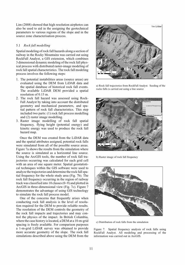
Spatial modeling of rock fall hazards along a section ofrailway in the Rocky Mountains was carried out usingRockFall Analyst, a GIS extension, which combines3 dimensional dynamic modeling of the rock fall phys-ical process with distributed raster-image modeling ofrock fall spatial characteristics. The rock fall modelingprocess involves the following steps:

1. The potential instabilities areas (source areas) areevaluated using the DEM from LiDAR data andthe spatial database of historical rock fall events.The available LiDAR DEM provided a spatialresolution of 0.15 m.

2. The rock fall hazard was assessed using Rock-Fall Analyst by taking into account the distributedgeometry and mechanical parameters, and spa-tial pattern of rock fall characteristics. This stepincluded two parts: (1) rock fall process modellingand (2) raster image modelling.

3. Raster image modelling of rock fall spatialfrequency, flying height (potential energy) andkinetic energy was used to produce the rock fallhazard map.

Once the DEM was created from the LiDAR dataand the spatial attributes assigned, potential rock fallswere simulated from all of the possible source areas.Figure 7a shows the results from the simulation wherethe source is simulated as a horizontal line source.Using the ArcGIS tools, the number of rock fall tra-jectories occurring was calculated for each grid cellwith an area of one square meter. Spatial geostatisti-cal techniques within the GIS software were used toanalyze the trajectories and determine the rock fall spa-tial frequency for the whole study area (Fig. 7b). Therock fall frequency occurring in the region of railwaytrack was classified into 10 classes (0–9) and plotted inArcGIS in three-dimensional view (Fig. 7c). Figure 7demonstrates the advantage of using GIS technologyto simulate the rock fall process model.

One of the concerns that frequently arises whenconducting rock fall analysis is the level of resolu-tion required for the DEM to provide reliable results.The resolution of the DEM controls the geometry ofthe rock fall impacts and trajectories and may con-trol the physics of the impact. In British Columbia,where the case history is located, a DEM at a 10-m-gridspacing is freely available. For comparison purposesa 1-m-grid LiDAR survey was obtained to providemore accurate geometry of the slope. The rock fallsimulations described above using the DEM from the

Figure 7. Spatial frequency analysis of rock falls usingRockFall Analyst. All modeling and processing of theinformation was carried out in ArcGIS.

11

Figure 8. Comparison of the historical rock fall frequencyimpacting the railway tracks with the results from the Rock-Fall Analyst simulations using the 1-m and 10-m digitalelevation models.

LiDAR survey were repeated using the 10-m DEM.Figure 8 compares the historical rock fall data baseto the results from RockFall Analysts for both the1-m and 10-m-grid. It is evident from Figure 8, thatthe rock fall simulations from the 1-m provides bet-ter agreement with the historical rock fall events (Lim2008).

5.2 Hazard zoning

Once the spatial distribution of the rock fall has beencomputed the energy from such events is required tocomplete the hazard assessment. Two raster layerswere created in ArcGIS to assess the spatial distri-bution of rock fall potential-energy (flying/bouncingheight relative to ground) and the kinetic energy(velocity). The energy raster layers combined with therock fall frequency is used to produce the rock fall haz-ard assessment shown in Figure 8. The rock fall hazardmap clearly identifies the section of railway with thegreatest risk, consistent with the historical evidence.Once the hazard has been identified, the energy rasterlayers can also be used to provide input to the designof protective barriers. Rock fall protection requiresan assessment of both the height (bouncing/flying)and velocity of the rock falls. Without such infor-mation the design of protective measures is usuallybased on single 2 dimensional analysis or qualitativemethods.

5.3 Summary

Rock falls are a significant hazard to Canadian rail-ways. The assessment of such hazards over longsections of railway requires an efficient means forstoring historical data and conducting rock fall sim-ulations. The development of the three dimensionalRockFall Analyst as an extension to ArcGIS, providesthe framework for rapid assessment of rock fall haz-ards. The use of such tools requires a detailed DEM

Figure 9. Rock fall hazard assessment based on rock fallfrequency and kinetic and potential energy.

as well as historical data for calibration purposes.Once calibrated, the energy output from RockFallAnalyst may be used in the design of protectivemeasures.

6 INTEGRATING GIS INTO GEOTECHNICALPRACTICE

Assessment of slope movement and associated hazardsdemands an understanding of the site characteristicsand their spatial and temporal variability. Currentgeotechnical modelling tools are focused on numeri-cal analyses and are not generally designed to facilitatethe requirements of site investigation and characteriza-tion. Site characterisation must address key geospatialissues, e.g., complex geology, highly irregular pore-water pressure, complex surface geometry and slipsurface definition as appropriate. There is little doubtthat capturing more complete geomorphological, geo-logical and geotechnical information improves thequality of geotechnical site investigation, particularlywhen the site is geologically and geotechnically com-plex (Luna & Frost 1998, Tsai & Frost 1999, Parsons &Frost 2002, Jaboyedoff et al. 2004, Kunapo et al.2005). Culshaw (2005) in the fifth Glossop lecturesuggested that ‘‘the rapid development in technol-ogy over the last twenty years and the digitizationof increasing amounts of geological data has broughtengineering geology to a situation in which the produc-tion of meaningful three-dimensional spatial modelsof the shallow subsurface is feasible’’. Despite theseadvances there are very few spatial tools that help thegeotechnical engineer achieve this goal.

12

While GIS is increasingly viewed as a key tool formanaging spatial distribution of data (Nathanail &Rosenbaum 1998, Parsons & Frost 2000, Kunapoet al. 2005) it has significant limitations in present-ing three-dimensional (3D) geologic and geotechnicaldata. Some GIS systems, like ArcGIS, developed bythe Environmental Systems Research Institute, Inc.(ESRI), provide a functional developer kit which canbe used to create 3D capability. However the cur-rent developments in 3D GIS are still not sufficientto meet the needs of the geotechnical engineer. Min-ing software such as Surpac Vision developed byGemcom Software International Incorporated pro-vide a comprehensive system for geological mod-elling but not geotechnical modelling. For example,while three-dimensional solid modelling and two-dimensional sections can be easily created in Sur-pac, querying inclinometer or piezometer data is notreadily accomplished. In the following section wedescribe an integrated approach using ArcGIS, Sur-pac Vision and numerical modeling, to develop athree-dimensional spatial model of a shallow sub-surface slide locally referred to as the Keillor RoadSlide. This integrated approach illustrates the addedvalue obtained when data and analyses are tightlyintegrated.

6.1 Development of an integrated approach

Nearly all slope site characterization efforts deal withsurface mapping, geological information from bore-hole data and monitoring data. The work flow fromdata collection through to engineering analyses wasoutlined by Lan & Martin (2007) and can be summa-rized in three stages (see Figure 1). Stage 1 involvesthe data collection, management and geosynthesisof the data. Modern GIS software provides effec-tive tools for the handling, integrating and visualizingdiverse spatial data sets (Brimicombe 2003). There-fore, in Stage 1, the functionality of GIS providesan essential role in collecting, storing, analyzing,visualizing and disseminating geospatial information.This information could be basic site investigationdata, such as geomorphology and geology condi-tions, and diverse, continually evolving geotechnicalparameters, such as displacement and pore pres-sure readings from geotechnical instruments. MostGIS tools have limitations in representing time seriesdata such as the displacement data from inclinome-ter or pore pressures from piezometers. Thereforeadditional functional tools were required for the stan-dard ArcGIS software. These tools have been imple-mented using ArcObject, an ArcGIS developer kit, andVisual studio.net, a software developing package byMicrosoft. These development tools provide capabil-ity for users to interact and communicate with variousdata sets.

The main aim of Stage 2 in Figure 1 is to establisha comprehensive ground model for the site. The con-struction of the ground model is enhanced using threedimensional geological modelling tools commonlyavailable in the mining industry.

Finally, geotechnical analyses and engineeringdecisions are performed in Stage 3 (see Figure 1).In this step the ground behaviour is analysed usingcommercially available geotechnical numerical tools.It is essential that the tools used in Stage 2 commu-nicate with the tools used in Stage 3 so that the dataintegration is maintained across all stages.

One of major issues in this integrated approachinvolves data input and output. In order to developan appropriate easy-to-use input and output function,some industrial standard file formats are employedfor data conversion and communication throughoutthe three Stages. Shape file (.SHP) from ESRI andData Exchange File (.DXF) from AutoDesk are bothindustrial standard formats supported by almost allPC-based CAD and GIS products. The communica-tion between different Stages in the system developedby Lan & Martin (2007) was implemented using thesetwo file formats.

The integration of the tools described above offerseffective digital tools to model heterogeneous geol-ogy, complex stratigraphy and slip surface geometry,and variable pore pressure conditions which are criticalto complex slope stability problems or other analyses.The tools also provide for incorporating findings frommonitoring data. In the following section the toolsare demonstrated using a translational bedrock slidein Edmonton Alberta.

6.2 Case study: Keillor Road slide

A complete description of the Keillor Road bedrockslide was given by Soe Moe et al. (2005). The failureof the slope occurred over a number of years with thelargest deformations occurring in 2002. The slide tookplace along the bank of the North Saskatchewan Rivervalley in Edmonton, Alberta Canada (Fig. 10). Thesite investigations for the slide were conducted overa period of 15 years using traditional boreholes andmonitoring systems.

Figure 11 shows a plan view of the site created inArcGIS indicating the outline of the slide, the topog-raphy of the area, location of the tension cracks andlocation of the main scarp. Figure 11 also shows thelocation of the boreholes that had been used in the siteinvestigations over the 15 year period. The major bene-fit of assembling the data in ArcGIS is that the boreholesymbols are dynamically linked to the data base andinstrumentation data installed in the boreholes.

To reconstruct the dynamics and kinematics ofthe processes acting on the slope and to determinetheir spatial and temporal distribution, Lan & Martin

13

Figure 10. Photograph of the Keillor Road Slide, from SoeMoe et al (2005).

Figure 11. Plan view of Keillor Road slope showing loca-tion of the site investigation boreholes, tension cracks andoutline of the slide. Contour elevations have been removedfor clarity.

(2007) developed add-on tools for the processing ofborehole information, plotting of time-series displace-ment data from slope inclinometers, pore pressuredata from piezometers and relative geomorphologi-cal features, such as tension cracks. The add-on toolsprovide all of the standard types of plots for analysingslope inclinometer data. From these standard plots dis-crete movement zones can be defined by specifyingthe from-to-depths. The resultant time-displacementplots for these discrete zones show acceleration or

deceleration of slope movement. In addition to thedisplacement versus time-plots, plots of displacementvector directions and displacement rate offer the abil-ity to identify and evaluate the spatial and temporalcharacter of the deformations, all in a user-friendlyenvironment.

In addition to being able to process the data quicklyin both a visual manner as well as conduct specificdepth queries, the user can quickly assess the kinemat-ics of the slide. Multiple movement zones at differentdepth are often detected in slope inclinometer plots. Inthis case, two movement zones were identified in theinclinometer readings for borehole B02-2 (Fig. 12).One zone was from depth 0.61 m to depth 2.44 m(zone 1) and the other zone was from depth 7.32 mto depth 8.53 m (zone 2). Their deformation historiescan be rapidly shown on the plan map (Fig. 12). Itcan be seen clearly that zones 1 and 2 show differentmovement characteristics. The moving direction of theshallow zone 1 changed direction frequently while thedirection of zone 2 was essentially unchanged.

Once the major rupture surface is identified, thespatial deformation pattern from all the inclinometer

Figure 12. Displacement history at different shear zones ofsite B02-2. Shearing zone 1 and zone 2 are characterized byobviously different displacement vectors.

14

data can be shown (Fig. 13). This provides a consis-tency check within the data sets as well highlightsthe more active portions of the slide as both totaldisplacements as well as displacement rate can beshown.

Geotechnical parameters are usually measured atpoints during site investigation by in-situ tests or bylaboratory tests. Geostatistical kriging and simula-tion techniques in GIS offer powerful spatial mod-eling tools for visualising the spatial variability ofthese parameters (Nathanail & Rosenbaum 1998).Parsons & Frost (2002) argued that such statisticalapproaches improve the quality of site investigationdata. Pore pressure is an essential parameter in slopestability studies. Lan & Martin (2007) used geosta-tistical techniques to interpret the point pore pressuredata into a spatial pore pressure surface. When con-ducting such geostatistical analysis it is important toensure that the pore pressures are being measured onthe same geological unit which can be readily verifiedby comparing the borehole logs and piezometer instal-lation locations. Lan & Martin (2007) also attached thethree dimensional displacement curves obtained fromthe inclinometer data to the boreholes as lines to showa spatial relationship between displacement locationsand pore pressure.

Figure 13. Spatial distribution of slope deformation fromall the inclinometer data at the same discrete movementzone. Two major slope portions with different displacementevolution are divided by Keillor Road.

As mentioned earlier, Surpac Vision providesadvanced tools for viewing and interpretation of geol-ogy data. Connecting to the same geological databaseas used by ArcGIS, the three-dimensional geologymodel for the Keillor Road Slide was created inSurpac Vision. Together with the other data importedfrom ArcGIS, such as the geomorphological surface,displacement and pore pressure readings, and tensioncrack planes, a comprehensive ground model for Keil-lor Road slope was created in Surpac Vision. Fromthe model, the spatial extent of the slope which is atrisk from instability can be immediately defined bythe displacement data and the surface mapping infor-mation. Critical profile sections can be extracted inSurpac Vision along the section lines parallel to thedisplacement vectors. These sections now include allinformation managed and produced in GIS and Sur-pac. These section profiles can be exported to DXFfiles which can then be optimized for slope stabilityanalysis. Nearly all modern slope stability softwaresuch as Slope/W or Slide can readily import DXF files.However, it is important that the user examine theseDXF files to ensure that the relevant information iscaptured.

Slope/W is widely used in geotechnical engineer-ing practice for analyzing the stability of slopes. It useslimit equilibrium theory to compute the critical factorof safety (Krahn 2003). The essential geometry ele-ments in Slope/W include the ground surface, complexgeological regions, and pore pressure line and tensioncrack lines. In many slope stability problems it is veryimportant to establish an accurate representation ofthe slope surface geometry because small changes inthe slope profile can have a significant impact on thecalculated factor of safety especially when the rupturesurface is relatively flat such as the translational slide atKeillor Road. Creating the section profile from LiDARsurvey ensures that the most accurate surface geome-try is captured. Figure 14 shows the final geometry andgeology modeled using Slope/W. The integration of the

Figure 14. Slope stability analysis using Limit equilibriumand/or Finite-element analysis.

15

GeoStudio Software means that this model can also beused for conducting deformation or stress analyses.

7 ANALYSING COMPLEX LANDSLIDES

In the previous section we showed the benefit of inte-grating technologies when analyzing a single slide.In this section we demonstrate the added value whenconsidering multiple complex landslides.

7.1 Background

Large translational landslides with rupture surfacesthrough glacial lake sediments in preglacial valleysare common hazards within river valleys of WesternCanada (Evans et al. 2005). Eleven, retrogressive,multiple, translational earth slides have occurred along10 kilometres of the Thompson River valley betweenthe communities of Ashcroft and Spences Bridge insouth-central British Columbia, Canada. The Cana-dian Pacific Railway (CPR) and Canadian NationalRailway (CN) main rail lines were constructed throughthe Thompson River valley in 1885 and 1905 respec-tively. Both have had recurring slope stability prob-lems along this valley (Fig. 15). Given that the twonational railroads traverse the same landslide pronearea, the evaluation of risk at this location is a matterof considerable significance.

The Ashcroft area is part of the Thompson Plateau,a subdivision of the Interior Plateau of BritishColumbia. The Thompson River flows south and

Figure 15. Major landslides south of Ashcroft, BC, (modi-fied from Eshraghian et al 2007).

has cut through about 150 metres of glacial sed-iments (Porter et al. 2002). Quaternary sedimentsoccur within the major valleys where deep valley fillshave been dissected and terraced by postglacial down-cutting of the trunk rivers. The landslides occurred onthe steep walls of an inner valley that formed duringthe Holocene when Quaternary sediments filling thebroader Thompson River valley were incised. The val-ley fill consists dominantly of permeable sediments,the exception being a unit of rhythmically-bedded siltand clay in the Pleistocene sequence (Clague & Evans2003). The surficial materials in the area are tills, flu-vial, fluvioglacial, lacustrine and colluvial deposits(Ryder 1976).

Individual investigations had been carried out forthe six most active of these earth slides in the Thomp-son Valley since the early 1980s. A major effortwas initiated in 2003 to re-analyse the data that hadbeen collected over the past 20 years using the spa-tial capabilities inherent in GIS tools. Eshraghianet al (2007) completed a comprehensive study of theslides and concluded that the rupture surfaces thathad been detected in the individual slides followed thehighly plastic, overconsolidated clays within a Pleis-tocene stratigraphic unit consisting of up to 45 metresof rhythmically-bedded glaciolacustrine deposit of siltand clay couplets, ranging from less than 1 cm toseveral tens of centimetres thick (Fig. 16). These sedi-ments may be several hundred thousand years old and

Figure 16. Geological units in the earth slides and highlandterraces in Thompson Valley. The arrows indicate the rupturesurfaces. Modified from Eshraghian et al 2007.

16

Figure 17. Example of an aerial photograph draped overa digital elevation model produced from an airborne Lidarsurvey (modified from Eshraghian et al 2007).

thus of Middle or Early Pleistocene age (Clague &Evans 2003). Samples of this unit from boreholes inSouth Slide show layers of brown, high-plastic clay1 to 20 cm thick between thicker layers of olive silt(Figure 16).

The deposits of the three glacial sequences areseparated by unconformities. Figure 16 shows thegeological succession synthesized from borehole logsand outcrops in scarps and terraces in the Ashcroftarea based on units proposed by Clague & Evans(2003). Eshraghian et al. (2007) used GIS technol-ogy to estimate the slide volumes which varied from1.8 to 21.4 Mm3 and spatially correlate the rupture sur-face. They concluded that the stratigraphic boundarieshave tilts of 1.7 m/km similar to the glacial lake bot-tom and that sliding was occurring along essentiallythe same layers within the glaciolacustrine sediments(Figure 16). They then examined the surface expo-sure of the larger slides using LiDAR technology.The airborne LiDAR provided a vertical resolution of±150 mm and when combined with the aerial pho-tographs illustrated the multiple blocks associated withretrogressive slides of this nature (Figure 17).

7.2 Multiblock retrogressive model

Eshraghian et al 2007 examined Slide CN50.9 usingtraditional site investigation boreholes and the com-bined Lidar DEM and aerial photograph model todevelop the geological and movement history sincedeglaciation (Fig. 18). During the first stage abraided Thompson River started cutting through theglacial sediments after deglaciation. Thompson Rivercontinued its down-cutting until it reached the firstweak layer and potential rupture surface (stage 2,Fig. 18). Progressive failure within this weak layercaused sliding of blocks A and B on the shallower rup-ture surface. More down-cutting by Thompson Riverencountered a deeper weak layer (Stage 3, Fig. 18).This time, movement happened without retrogres-sion on the deeper rupture surface. It caused more

Figure 18. Simplified multiblock model illustrating thesliding process since deglaciation at the Slide CN50.9 (mod-ified from Eshraghian et al 2007).

horizontal movement by block A and horizontal andvertical movement by block B. This sliding and also theThompson River erosion caused progressive failure onthe deeper rupture surface and the slide was ready foranother retrogression (Stage 4, Figure 18). The mostrecent retrogression of the Slide CN50.9 happened inSeptember 1897. During this stage, block D moveddown on the main scarp and rest of slide materialmoved horizontally toward the river (Stage 5, Fig. 4).During this retrogression in the early morning ofSeptember 22, 1897, residents of Ashcroft were awak-ened by loud, thunder-like rumblings. The landslideconstricted the Thompson River without completelyblocking it (Clague & Evans 2003). From these expla-nations, the movement rate during this retrogressionis estimated to be rapid. Following the slide, Thomp-son River removed part of the toe of the slide, mainlywithin block A (stage 6, Figure 18).

Eshraghian et al 2007 used the conceptual modeldeveloped in Figure 18 to develop the geologicalmultiblock model for the retrogressive slide shown

17

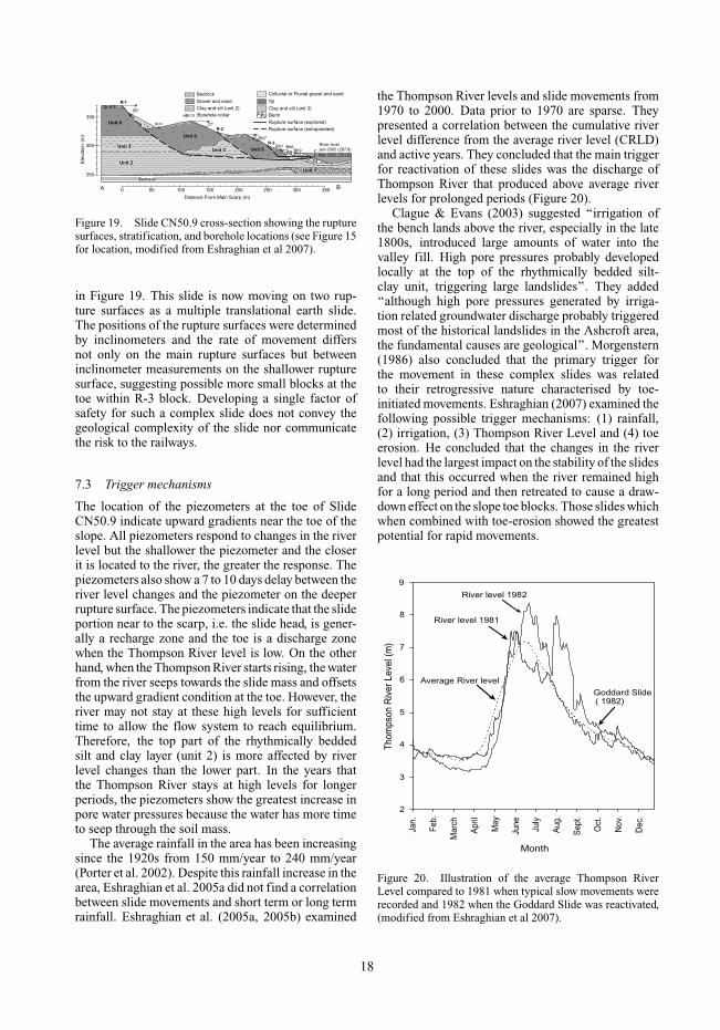
Figure 19. Slide CN50.9 cross-section showing the rupturesurfaces, stratification, and borehole locations (see Figure 15for location, modified from Eshraghian et al 2007).

in Figure 19. This slide is now moving on two rup-ture surfaces as a multiple translational earth slide.The positions of the rupture surfaces were determinedby inclinometers and the rate of movement differsnot only on the main rupture surfaces but betweeninclinometer measurements on the shallower rupturesurface, suggesting possible more small blocks at thetoe within R-3 block. Developing a single factor ofsafety for such a complex slide does not convey thegeological complexity of the slide nor communicatethe risk to the railways.

7.3 Trigger mechanisms

The location of the piezometers at the toe of SlideCN50.9 indicate upward gradients near the toe of theslope. All piezometers respond to changes in the riverlevel but the shallower the piezometer and the closerit is located to the river, the greater the response. Thepiezometers also show a 7 to 10 days delay between theriver level changes and the piezometer on the deeperrupture surface. The piezometers indicate that the slideportion near to the scarp, i.e. the slide head, is gener-ally a recharge zone and the toe is a discharge zonewhen the Thompson River level is low. On the otherhand, when the Thompson River starts rising, the waterfrom the river seeps towards the slide mass and offsetsthe upward gradient condition at the toe. However, theriver may not stay at these high levels for sufficienttime to allow the flow system to reach equilibrium.Therefore, the top part of the rhythmically beddedsilt and clay layer (unit 2) is more affected by riverlevel changes than the lower part. In the years thatthe Thompson River stays at high levels for longerperiods, the piezometers show the greatest increase inpore water pressures because the water has more timeto seep through the soil mass.

The average rainfall in the area has been increasingsince the 1920s from 150 mm/year to 240 mm/year(Porter et al. 2002). Despite this rainfall increase in thearea, Eshraghian et al. 2005a did not find a correlationbetween slide movements and short term or long termrainfall. Eshraghian et al. (2005a, 2005b) examined

the Thompson River levels and slide movements from1970 to 2000. Data prior to 1970 are sparse. Theypresented a correlation between the cumulative riverlevel difference from the average river level (CRLD)and active years. They concluded that the main triggerfor reactivation of these slides was the discharge ofThompson River that produced above average riverlevels for prolonged periods (Figure 20).

Clague & Evans (2003) suggested ‘‘irrigation ofthe bench lands above the river, especially in the late1800s, introduced large amounts of water into thevalley fill. High pore pressures probably developedlocally at the top of the rhythmically bedded silt-clay unit, triggering large landslides’’. They added‘‘although high pore pressures generated by irriga-tion related groundwater discharge probably triggeredmost of the historical landslides in the Ashcroft area,the fundamental causes are geological’’. Morgenstern(1986) also concluded that the primary trigger forthe movement in these complex slides was relatedto their retrogressive nature characterised by toe-initiated movements. Eshraghian (2007) examined thefollowing possible trigger mechanisms: (1) rainfall,(2) irrigation, (3) Thompson River Level and (4) toeerosion. He concluded that the changes in the riverlevel had the largest impact on the stability of the slidesand that this occurred when the river remained highfor a long period and then retreated to cause a draw-down effect on the slope toe blocks. Those slides whichwhen combined with toe-erosion showed the greatestpotential for rapid movements.

Figure 20. Illustration of the average Thompson RiverLevel compared to 1981 when typical slow movements wererecorded and 1982 when the Goddard Slide was reactivated,(modified from Eshraghian et al 2007).

18

7.4 Movement and risk

It is obvious from the discussion above that attempt-ing to capture the risk from the movement associatedwith such landslides with a single number is not prac-tical. Eshraghian et al 2007 used a quantitative hazardanalysis in a framework that considered the differ-ent post-failure movement rates. They demonstratedthe approach using probabilistic stability analysesthat included material and trigger uncertainties as

Figure 21. Thompson River level for different yearly dis-charge return periods.

Figure 22. Histogram frequency distribution of movementrate for two translational blocks on shallower and deeperrupture surfaces.

well as uncertainties from the groundwater modelingand toe erosion. The probabilistic rates of movementwere calculated using the frequency of the trigger(the Thompson River flood, Figure 21), the historicmovement rates, for each reactivation block.

The result of calculating the probability ofmovement for reactivation blocks are a movementprobability distribution (Figure 22) which shows theprobability distribution of different movement rateswhich may happen during the design life time of theproject. They also reported the results for each reac-tivation block in the form of probability of differentmovement rates using the movement rate class sug-gested by Cruden & Varnes (1996) calculated for thedesigned life time of 100 years (Fig. 23).

7.5 Summary

The Introduction for this paper drew attention tothe large number of contributory processes that haveto be considered in developing an effective processmodel of a landslide and its consequences. All ofthese contributory processes have had to be consid-ered in the example just presented; from geology andgeomorphology through hydrological and geotechni-cal characterization and finally geotechnical and risk

Figure 23. Frequency of different movement rate classesfor reactivation blocks defined within Slide CN50.9 for a100 year return period.

19

analyses, utilizing both deterministic and probabilis-tic considerations. The capacity for undertaking suchcomplex landslide analyses was enhanced by the avail-ability of recently developed tools such as LiDARimagery. However, it is unlikely that the end productcould have been achieved without utilizing GIS forspatial data management, correlations and analysis.

8 CONCLUDING REMARKS

A number of recent technical advances are leadingto dramatic improvements in the study of landslidesand the evaluation of appropriate risk mitigationmeasures. This paper draws attention to some, suchas the application of LiDAR to delineate landslidesmore clearly than aerial photographs, and the role ofInSAR to monitor ground movements over large areaswith increasing accuracy. A number of other tools areentering practice that merit discussion but were beyondthe scope of this paper.

It has been the central premise of this paper thatthe most important advances have been associatedwith improved visualization of landslides and relatedprocesses, both through surface and sub-surface fea-tures. To this end, our experience leads us to theview that GIS is capable of making transformativecontributions.

Examples of use of GIS in geotechnical assessment,beyond its routine application of archiving surfaceinformation, have been provided. A general rockfallsimulation model has been developed with GIS. Otherexamples illustrate the integration of GIS with subsur-face modelling capability with interfaces to any kindof geotechnical analysis software.

Landslide data management and analysis of allkinds in GIS will be essential for future progress inlandslide engineering as three-dimensional visualiza-tion and modelling capabilities improve.

ACKNOWLEDGMENTS

The authors wish to acknowledge the assistance of thefollowing:

i. Dr. Hengxing Lan, Research Engineer, for hisleadership in developing GIS based tools at theUniversity of Alberta.

ii. Mr. Cory Froese, Team Leader—Geological Haz-ards, Alberta Geological Survey/Energy and Util-ities Board, for assisting us with understandingthe current status of InSAR applied to landslidestudies.

iii. The graduate students who have collaborated withus in these and related studies over the past fewyears.

iv. The Gateway Pipeline Project for providingFigure 3.

The development of the ArcGIS tools and thecase histories described in this paper was supportedby the Canadian Railway Ground Hazard ResearchProgram, a collaborative research program betweenCanadian National Railway, Canadian Pacific Rail-way, Transport Canada, Geological Survey of Canada,University of Alberta, Queen’s University and theNatural Sciences and Engineering Council of Canada.

REFERENCES

Agliardi, F. & Crosta, G.B. 2003. High resolution three-dimensional numerical modelling of rockfalls. Interna-tional Journal of Rock Mechanics and Mining Science40 (4): 455–471.

Ardizzone, F., Cardinali, M., Gzzetti, F. & Reichen-bach, P. 2007. Identification and mapping of recentrainfall-induced landslides using elevation data collectedby airborne LiDAR. Natural Hazards and Earth SystemSciences 7: 637–650.

Bjerrum, L. 1967. Progressive failure in slopes andoverconsolidated plastic clay and clay shales. JournalSoil Mechanics and Foundations Division, ASCE 93(SM5): 3–49.

Brimicombe, A. 2003. GIS, Environmental modelling andengineering, London; N.Y.: Taylor & Francis, 312 p.

Carter, W.E., Shresthe, R.L. & Slatton, K.C. 2007. Geodeticlaser scanning. Physics Today 60: 41–47.

Chacón, J., Irigaray, C., Fernandez, T. & El Hamdouni, R.2006. Engineering geology maps: landslides and geo-graphical information systems. Bulletin of EngineeringGeology and the Environment 65: 341–411.

Chandler, J.H. & Brunsden, D. 1995. Steady statebehaviour of the Black Ven mudslide: the application ofarchival analytical photogrammetry to studies of land-form change. Earth Surface Process and Landforms20: 255–275.

Clague, J.J. & Evans, S.G. 2003. Geological framework oflarge historic landslides in Thompson River Valley, BritishColumbia. Environmental and Engineering Geoscience9: 201–212.

Colesanti, C. & Wasowski, J. 2006. Investigating Land-slides with Space-borne Synthetic Aperture Radar (SAR)Interferometry. Engineering Geology 88: 173–199.

Cruden, D.M. & Varnes, D.J. 1996. Landslide types andprocesses. Transportation Research Board Special report247: 36–75.

Culshaw, M.G. 2005. The Seventh Glossop Lecture—Fromconcept towards reality: developing the attributed 3Dgeological model of the shallow subsurface QuarterlyJournal of Engineering Geology and Hydrogeology 38:231–284.

Cunningham, D., Grebby, S., Tansey, K., Gosar, A. &Kastelic, V. 2006. Application of air borne LiDAR tomapping seismogenic faults in forested mountainous ter-rain, southeastern Alps, Slovenia. Geophysical ResearchLetters 33: L20308.

20

Dai, F.C. & Lee, C.F. 2004. A spatiotemporal probabilis-tic modelling of storm-induced shallow landsliding usingaerial photographs and logistic regression. Earth SurfaceProcesses and Landforms 28: 527–545.

Delmonaco, G., Leoni, G., Margottini, C., Puglisi, C. &Spizzichino, D. 2003. Large scale debris-flow hazardassessment: a geotechnical approach and GIS mod-elling. Natural Hazards and Earth System Sciences3: 433–455.

Dietrich, W.E. & Montgomery, D.R. 1998. A digital terrainmodel for mapping shallow landslide potential. TechnicalReport NCASI. http://socrates.berkeley.edu/∼geomorph/shalstab/

Dorren, L.K.A. & Seijmonsbergen, A.C. 2003. Comparisonof three GIS-based models for prediction rock fall runoutzones at a regional scale. Geomorphology 56: 49–64.

Eshraghian, A. 2007. Hazard analysis of reactivated earthslides along the Thompson River Valley, Ashcroft, BritishColumbia. PhD Thesis Dept. Civil & EnvironmentalEngineering, University of Alberta, Edmonton, Alberta,Canada.

Eshraghian, A., Martin, C.D. & Cruden, D.M. 2005a. Land-slides in the Thompson River valley between Ashcroft andSpences Bridge, British Columbia. In Proceedings of theInternational Conference on Landslide Risk Management,Vancouver, Canada, May 31 to June 4, 2005: 437–446.s

Eshraghian, A., Martin, C.D. & Cruden, D.M. 2005b. Earthslide movements in the Thompson River valley, Ashcroft,British Columbia. In Proceedings of the 58th Cana-dian Geotechnical Conference, Saskatoon, Saskatchewan,Canada, September 18–21, 2005.

Eshraghian, A., Martin, C.D. & Cruden, D.M. 2007. Com-plex Earth Slides in the Thompson River Valley, Ashcroft,British Columbia. Environmental and Engineering Geo-science Journal XIII: 161–181.

Evans, S.G., Cruden, D.M., Brobrowsky, P.T., Guthrie,R.H., Keegan, T.R., Liverman, D.G.E. & Perret, D.2005. Landslide risk assessment in Canada; a review ofrecent developments. In Proceedings of the InternationalConference on Landslide Risk Management, Vancouver,Canada, 31 May–3 June 2005. A.A. Balkema. 351–434.

Farina, P., Casgli, N. & Ferretti, A. 2007. Radar-Interpretation of InSAR Measurements for LandslideInvestigations in Civil Protection Practices. In Schaefer,V.R., Schuster, R.L., Turner, A.K. (eds), Landslides andSociety. AEG Special Publication 23: 272–283.

Farina, P., Colombo, D., Fumagalli, A., Marks, F. &Moretti, S. 2006. Permanent scatterers for landslideinvestigations: Outcomes from the ESA-SLAM Project.Engineering Geology 88: 200–217.

Ferretti, A., Prati, C. & Rocca, F. 1999. Permanent scat-terers in SAR interferometry. International Geoscienceand Remote Sensing Symposium, Hamburg, Germany, 28June-2 July, 1999. 1–3.

Ferretti, A., Prati, C. & Rocca, F. 2000. Nonlinear subsidencerate estimation using permanent scatterers in differentialSAR interferometry. IEEE Transactions on Geoscienceand Remote Sensing 38(5): 2202–2212.

Ferretti, A., Prati, C. & Rocca, F. 2001. Permanent scatterersin SAR interferometry. IEEE Transactions on Geoscienceand Remote Sensing 39(1): 8–20.

Findley, D.P. 2007. Rock Stars. Civil Engineering July:46–51.

Franks, C.A., Koor, N.P. & Campbell, S.D.G. 1998. An inte-grated approach to the assessment of slope stability inurban areas in Hong Kong using thematic maps. Proc 8thIAEG Congress. Vancouver: Balkema, 1103–1111.

Froese, C.R., Kosar, K. & van der Kooij, M. 2004. Advancesin the application of InSAR to complex, slowly movinglandslides in dry and vegetated terrain; in Landslides:Evaluation and Stabilization, W. Lacerda, M. Erlich,S.A.B. Fontoura & A.S.F. Sayao (ed.), Proceedings of the9th International Landslide Symposium, Rio de Janeiro,Brazil: 1255–1264.

Froese, C.R., Poncos, V., Skirrow, R., Mansour, M. &Martin, C.D. 2008. Characterizing Complex Deep SeatedLandslide Deformation using Corner Reflector InSAR(CR-INSAR): Little Smoky Landslide, Alberta. Proceed-ings of the 4th Canadian Conference on Geohazards.Quebec: In Press.

Günther, A., Carstensen, A. & Pohl, W. 2004. Automatedsliding susceptibility mapping of rock slopes. NaturalHazards and Earth Systems Sciences 4: 95–102.

Guzzetti, F., Crosta, G., Detti, R. & Agliardi, F. 2002.STONE: a computer program for the three-dimensionalsimulation of rock-falls. Computers & Sciences 28:1079–1093.

Harries, N.J. & Roberts, H. 2007. The use of slope stabil-ity radar (SSR) in managing slope instability hazards. InEberhardt, E., Stead, D. & Morrison, T. (eds), Proceedings1st Canada-U.S. Rock Mechanics Symposium, Vancouver1: 53–59. London: Taylor & Francis Group.

Haugerud, R.A., & Harding, D.J. 2001. Some algorithmsfor virtual deforestation (VDF) of lidar topographic sur-vey data. International Archives of Photogrammetry andRemote Sensing 34–3/W4: 211–217.

Hong, Y., Adler, R.F. & Huffman, G.J. 2007. Satel-lite remote sensing for global landslide monitoring,EDS. Transactions of the American Geophysical Union88: 357.

Jaboyedoff, M., Ornstein, P. & Rouiller, J.-D. 2004. Designof a geodetic database and associated tools for monitoringrock-slope movements: the example of the top of Randarockfall scar. Natural Hazards and Earth System Sciences4: 187–196 (pdf, 5755 Ko).

Jaboyedoff, M., Metzger, R., Oppikofer, T., Coulture, R.,Derron, M., Locat, J. & Turmel, D. 2007. New insighttechniques to analyse rock slope relief using DEM and3D-imaging cloud points: COLTOP-3D software, In Eber-hardt, E., Stead, D. & Morrison, T. (eds), Proceedings 1stCanada-U.S. Rock Mechanics Symposium, Vancouver 1:61–68. London: Taylor & Francis Group.

Jones, C.L., Higgins, J.D., & Andrew, R.D. 2000. ColoradoRock fall Simulation Program Version 4.0. ColoradoDepartment of Transportation. Colorado Geological Sur-vey, March 2000. 127 pp.

Kemeny, J., Norton, B. & Turner, K. 2006. Rock slope sta-bility analysis utilizing ground-based LiDAR and digitalimage processing. Felsbau 24: 8–16.

Krahn, J. 2003. The 2001 R.M. Hardy Lecture: The lim-its of limit equilibrium analyses. Canadian GeotechnicalJournal 40(3): 643–660.

Kunapo, J., Dasari, G.R., Phoon, K.K. & Tan, T.S. 2005.Development of a Web-GIS based geotechnical informa-tion system. Journal of Computing in Civil Engineering19(3): 323–327.

21

Lan, H.X., Lee, C.F., Zhou, C.H. & Martin, C.D. 2005.Dynamic characteristics analysis of shallow landslidesin response to rainfall event using GIS. EnvironmentalGeology 47(2): 254–267.

Lan, H. & Martin, C.D. 2007. A digital approach forintegrating geotechnical data and stability analyses inE.Eberhardt, D. Stead & Morrison, T. (eds), Rock Mech-nanics: Meeting Society’s Challenges and Demands,45–2. London: Taylor and Francis Group.

Lan, H., Martin, C.D. & Lim, C.H. 2007. Rockfall Ana-lyst: a GIS extension for three-dimensional and spa-tially distributed rockfall hazard modelling. Computers &Geosciences 33: 262–279.

Lim, C.H. 2008. A process model for rock fall, PhD ThesisDept. Civil & Environmental Engineering, University ofAlberta, Edmonton, Canada.

Luna, R. & Frost, J.D. 1998. Spatial liquefaction analysis sys-tem. Journal of Computing in Civil Engineering 12 (1):48–56.

Maffei, A., Martino, S. & Prestininzi, A. 2005. From thegeological to the numerical model in the analysis ofgravity-induced slope deformations: An example from theCentral Apennines (Italy). Engineering Geology 78(3–4):215–236.

Martin, C.D., Tannant, D.D. & Lan, H. 2007. Comparisonof terrestrial-based, high resolution, LiDAR and digitalphotogrammetry surveys of a rock slope. Eberhardt, E.Stead, D. & Morrison, T. (eds), Proceedings 1st Canada-U.S. Rock Mechanics Symposium, Vancouver. Taylor &Francis Group, London 1: 37–44.

McCardle, A., Rabus, B., Ghuman, P., Rabaco, L, M.L.,Amaral, C.S. & Rocha, R. 2007. Using Artificial PointTargets for Monitoring Landslides with InterferometricProcessing. Anais XIII Simposio Brasileiro de Sensoria-mento Remoto. INPE: 4933–4934.

Meisina, C., Zucca, F., Conconi, F., Verri, F., Fossati, D.,Ceriani, M. & Allievi, J. 2007. Use of Permanent Scatter-ers Technique for Large-scale Mass Movement Investiga-tion. Quaternary International 171–172: 90–107.

Mejia-Navarro, M., Wohl, E.W. & Oaks, S.D. 1994. Geologi-cal hazards, vulnerability, and risk assessment using GIS:model for Glenwood Springs, Colorado. Geomorphology43: 117–136.

Morgenstern, N.R. 1986. Goddard landslide of September,1982, summary of the opinion of Norbert R. Morgenstern.Report prepared for court between Canadian PacificLimited and Highland Valley Cattle Company Limited.Supreme Court of British Columbia: Vancouver registryNo. C841694.

Morgenstern, N.R. 2000. Performance in geotechnical prac-tice: Inaugural Lumb Lecture. Transactions Hong KongInstitute of Engineers 7: 1–15.

Nathanail, C.P. & Rosenbaum, M.S. 1998. Spatial manage-ment of geotechnical data for site selection. EngineeringGeology 50(3–4): 347–356.

Parise, M. 2003. Observations of surface features on an activelandslide and implications for understanding its history ofmovement. Natural Hazards and Earth System Sciences3: 569–580.

Parsons, R.L. & Frost, J.D. 2000. Interactive analy-sis of spatial subsurface data using GIS-Based tool.Journal of Computing in Civil Engineering 14(4):215–222.

Parsons, R.L. & Frost, J.D. 2002. Evaluating site investigationquality using GIS and geostatistics. Journal of Geotechni-cal and Geoenvironmental Engineering 128 (6): 451–461.

Pfeiffer, T.J. & Bowen, T. 1989. Computer simulation ofrock falls. Bulletin of the Association of EngineeringGeologists 26 (1): 135–146.

Porter, M.J., Savigny, K.W., Keegan, T.R., Bunce, C.M. &MacKay, C. 2002. Controls on stability of the ThompsonRiver landslides. In Proceedings 55th Canadian Geotech-nical Conference: Ground and Water: Theory to Practice,Niagara Falls, Ontario, Vol. 2 , pp 1393–1400.

Pötsch, M., Schubert, W. & Gaich, A. 2007. The applica-tion of metric 3D images for the mechanical analysis ofkeyblocks. In Eberhardt, E., Stead, D. & Morrison, T.(eds), Proceedings 1st Canada-U.S. Rock Mechanics Sym-posium, Vancouver 1: 77–84. London: Taylor & FrancisGroup.

Radbruch, D.H. & Crowther, K.C. 1973. Map showing areasof estimated relative susceptibility to landsliding in Cal-ifornia. U.S. Geological Survey, Miscellaneous GeologicInvestigation Map I-747.

Refice, A. & Capolongo, O. 2002. Probabilistic modellingof uncertainties in earthquake-induced landslide hazardassessment. Computing and Geoscience 28: 735–749.

Rhina, D. 1992. Why GIS? ARC News 11: 1–4.Rizkalla, M. & Randall, C. 1999. A Demonstration of

Satellite-Based Remote Sensing Methods for GroundMovement Monitoring in Pipeline Integrity Management.Proceedings 18th International Conference on OffshoreMechanics and Arctic Engineering. St. John’s, OMAE99/PIPE-5004, ASME.

Rosser, N.J., Petley, D.N., Lim, M., Dunning, S.A. &Allison, R.J. 2005. Terrestrial laser scanning for monitor-ing the process of hard rock coastal cliff erosion. Quar-terly Journal of Engineering Geology and Hydrogeology38: 363–373.

Ryder, J.M. 1976. Terrain inventory and Quaternary geol-ogy, Ashcroft, British Columbia, Geological Survey ofCanada, Ottawa.

Schulz, W.H. 2004. Landslides mapped using LiDARimagery, Seattle, Washington. U.S. Geological Survey,Open-File Report 2004-1396.

Schulz, W.H. 2007. Landslide susceptibility revealed byLiDAR imagery and historical records, Seattle, Washing-ton. Engineering Geology 89: 67–87.

Singhroy, V. 2005. Remote sensing of landslides. In Glade, T.,Anderson, M. & Crozier, M.J. (eds), Landslide Hazardand Risk 469–492. Wiley.

Soe Moe, K.W., Cruden, D.M., Martin, C.D., Lewycky,D. & Lach, P.R. 2005. 15 years of movement at KeillorRoad, Edmonton. Proceedings 58th Canadian Geotechni-cal Conference & 6th Joint CGS/IAH-CNC GroundwaterSpecialty Conference, Saskatoon, 1: 281–388.

Soeters, R. & Van Westen, C.J. 1996. Slope instability, recog-nition, analysis, and zonation in Turner, A.K. and Schus-ter, R.L. (eds). Landslides: Investigation and Mitigation129–177. Washington, D.C.: National Academy Press.

Sturznegger, M., Stead, D., Froese, C., Moreno, F. & Jaboyed-off, M. 2007. Ground-based and airborne LiDAR forstructural mapping of the Frank Slide. In Eberhardt, E.,Stead, D. & Morrison, T. (eds), Rock Mechanics: Meet-ing Society’s Challenges and Demands 925–932. London:Taylor and Francis.

22

Tsai, Y.C. & Frost, J.D. 1999. Using geographic informationsystem and knowledge base system technology for real-time planning of site characterization activities. CanadianGeotechnical Journal 36 (2): 300–312.

Van Westen, C.J. & Getahun, F.L. 2003. Analyzing theevolution of the Tessina landslide using aerial photo-graphs and digital elevation models. Geomorphology54: 77–89.

Van Westen, C.J. 2007. Mapping landslides: Recent devel-opments in the use of the digital spatial information.Proceedings 1st North American Landslide Conference,Vail, CO 221–238.

Varnes, D.J. 1984. International Association of Engineer-ing Geology Commission on Landslides and Other MassMovements on Slopes. Landslide Hazard Zonation. Inter-national Association of Engineering Geology. UNESCONatural Hazard Series 3(63) pp.

Wachal, D.J. & Hudak. P.F. 2000. Mapping landslide sus-ceptibility in Travis County, Texas, USA. GeoJournal 51:245–253.

Walstra, J., Dixon, N. & Chandler, J.H. 2007. Historicalaerial photographs for landslide assessment: two case his-tories. Quarterly Journal of Engineering Geology andHydrogeology 40: 315–332.

23