lappeenranta university of technology ltkk
TRANSCRIPT
f* 3 ATkLL- -- A 31
LAPPEENRANNAN TEKNILLINEN KORKEAKOULUEnergiatekniikan osasto
LAPPEENRANTA UNIVERSITY OF TECHNOLOGY Department of Energy Technology
RESEARCH REPORT EN A-33
LTKK
DESIGN OF A SWITCHED RELUCTANCE GENERATOR
Thomas Heese Juha Pyrhonen
FOREIGN SALES PROHIBITED
1996
%
ISBN 951-764-077-3 ISSN 0785-823X
H
DISTRIBUTION RESTRICTED TO U S. ONLY '»

DISCLAIMER
Portions of this document may be illegible electronic image products. Images are produced from the best available original document.

ABSTRACTLAPPEENRANTA UNIVERSITY OF TECHNOLOGY
Department of Energy Technology Section of Electric Power Engineering
Thomas Heese, researcherJuha Pyrhonen, associate professor, doctor of technology
DESIGN OF A SWITCHED RELUCTANCE GENERATORLUT, Department of Energy Technology, September 1996, 105 pages, 61 pictures, 10 tables, 1 appendix
Research Report EN A-33
ISBN 951-764-077-3 ISSN 0785-823X UDK: 621.313
Key Words: Electrical Machines, Switched Reluctance Machines, Generators
This paper presents the design of a low voltage switched reluctance generator for variable speed applications showing the design of its construction and commutation unit. For the realisation of the control system the control strategy is presented. The principle and the theory of switched reluctance generators are described in this context. Also an overview of existing generator technology for these applications is given.
The results gained suggest that switched reluctance machines can also advantageously be used as generators if the generating operation is considered within the design process. Compared with the existing technology a higher output power and efficiency is reached over the whole speed range.
Lappeenranta, September 1996
Thomas Heese, Juha Pyrhonen
J

2
Contents
Preface.............................................................................................................................................1
Contents..........................................................................................................................................2
List of Symbols.............................................................................................................................4Tiivistelma...................................................................................................................................... 9
1 Introduction...........................................................................................................................10
2 Generators for Variable Speed Applications..................................................................12
2.1 DC Generator............................................................................................................... 13
2.2 Alternator....................................................................................................................... 15
2.3 Weak Spots of Existing Technology........................................................................18
2.4 Supposed Improvements and Advantages of Switched Reluctance Technology21
3 Principle and Theory of Switched Reluctance Generators......................................... 24
3.1 Construction................................................................................................................. 24
3.1.1 Basic Characteristics........................................................................................... 25
3.1.2 Envelope and Internal Dimensions.................................................................. 27
3.1.3 Pole Geometry.....................................................................................................30
3.1.4 Windings............................................................................................................... 32
3.2 Working Principle........................................................................................................32
3.2.1 Rotor Position Dependency............................................................................... 33
3.2.2 Torque and Currents.......................................................................................... 37
3.2.3 Mathematical Description.................................... 39
3.2.4 Energy Conversion............................................................................................. 41
3.3 Commutation Unit.....................................!................................................................ 46
3.3.1 Classic Converter................................................................................................47
3.3.2 (»+l)-switch converter..................................................... :...............................48
3.3.3 Boost and Buck Converter............................................................................... 49
3.3.4 Bifilar Winding Converter..................................................................................51
3.3.5 Other Converter Topologies............................................................................. 52
3.4 Dynamic Operation......................................................................................................52
3.4.1 Single-Pulse Operation....................................................................................... 53
3.4.2 Chopping.............................................................................................................. 55
3.5 Control System.............................................................................................................55
3.5.1 Structure............................................................................................................... 56
3.5.2 Control Modes and Strategy.............................................................................56
3.5.3 Sensorless Control...............................................................................................58
Contents 3
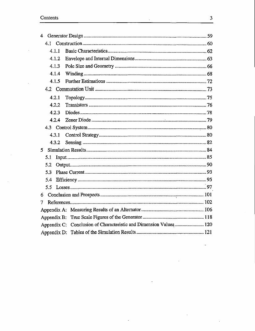
4 Generator Design................................................................................................................ 59
4.1 Construction................................................................................................................. 60
4.1.1 Basic Characteristics............................................................................................62
4.1.2 Envelope and Internal Dimensions................................................................... 63
4.1.3 Pole Size and Geometry......................................................................................66
4.1.4 Winding................................................................................................................. 68
4.1.5 Further Estimations............................................................................................ 72
4.2 Commutation Unit................................................................................................. 73
4.2.1 Topology................................................................................................................75
4.2.2 Transistors............................................................................................................ 76
4.2.3 Diodes.................................................................................................................... 78
4.2.4 Zener Diode................................................................... 79
4.3 Control System....................................................................................................... 80
4.3.1 Control Strategy................................................................................................... 80
4.3.2 Sensing.................................................................................................................. 82
5 Simulation Results...............................................................................................................845.1 Input...............................................................................................................................85
5.2 Output..............................................................................................................................90
5.3 Phase Current................................................................................................................93
5.4 Efficiency.......................................................................................................................95
5.5 Losses..............................................................................................................................97
6 Conclusion and Prospects...................................................................... 101
7 References............................................................................................................................102
Appendix A: Measuring Results of an Alternator.........................................................106
Appendix B: True Scale Figures of the Generator....................................................... 118
Appendix C: Conclusion of Characteristic and Dimension Values..........................120
Appendix D: Tables of the Simulation Results..........................................................121
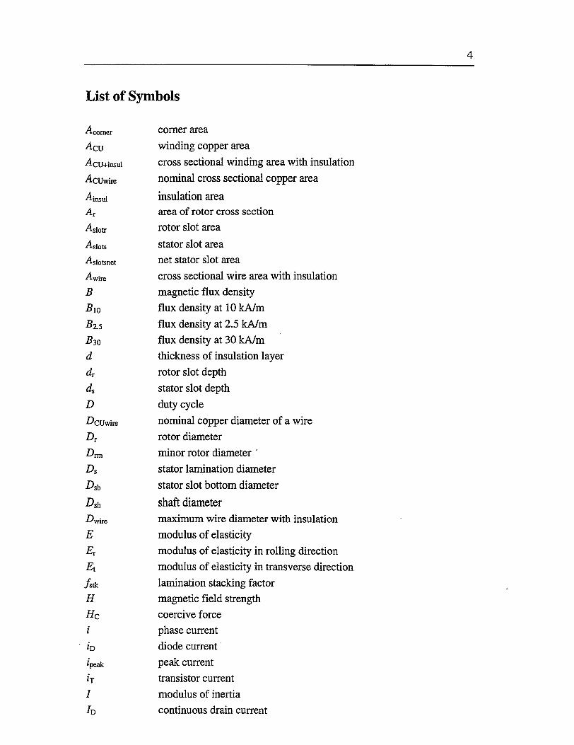
List of Symbols
•'i comer
AcuAcu+insul
Acu wire
Ainsul
ArAglotr
AglotS
Aslotsnet
A wire
B•BioB2.5
B30ddrdsD•DcUwireDrDrmDsDsbDSh•Dwire
EErEtfstk
HHei
bzpeak
hIb
comer area winding copper areacross sectional winding area with insulation
nominal cross sectional copper area
insulation areaarea of rotor cross sectionrotor slot area
stator slot areanet stator slot areacross sectional wire area with insulationmagnetic flux densityflux density at 10 kA/mflux density at 2.5 kA/mflux density at 30 kA/mthickness of insulation layerrotor slot depthstator slot depthduty cycle
nominal copper diameter of a wire rotor diameter minor rotor diameter ' stator lamination diameter
stator slot bottom diameter
shaft diametermaximum wire diameter with insulationmodulus of elasticitymodulus of elasticity in rolling directionmodulus of elasticity in transverse directionlamination stacking factormagnetic field strengthcoercive forcephase currentdiode currentpeak currenttransistor currentmodulus of inertiacontinuous drain current
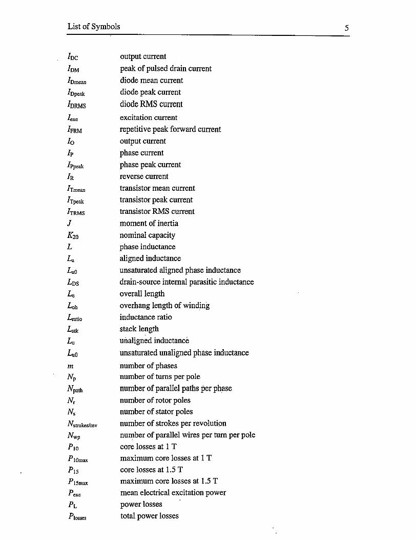
List of Symbols 5
Idc output currentIdm peak of pulsed drain currentfomean diode mean current■fopeak diode peak current^DRMS diode RMS current
■lexc excitation currentfpRM repetitive peak forward currentIo output currenth phase currentfppeak phase peak current/r reverse current■^Tmean transistor mean current■^Tpeak transistor peak current/trms transistor RMS currentJ moment of inertiaK20 nominal capacityL phase inductanceU aligned inductanceLaO unsaturated aligned phase inductanceLds drain-source internal parasitic inductanceu overall lengthLoh overhang length of windingLratio inductance ratioLstk stack lengthLu unaligned inductanceLuO unsaturated unaligned phase inductance
m number of phasesNp number of turns per poleNpalh number of parallel paths per phaseNr number of rotor polesNs number of stator polesNstrokes/rev number of strokes per revolutionMvp number of parallel wires per turn per poleP10 core losses at 1 Tf lOmax maximum core losses at 1 TPl5 core losses at 1.5 TP ISmax maximum core losses at 1.5 Tfexc mean electrical excitation powerPl power lossesPlosses total power losses

List of Symbols 6
P mech
•Pout
Pshaft
Pjpeak
rRP wiremax
P wiremin
RoRiPiP3T?DS(on)
PphDC
PshPthjc
Sfill^fillinsul
t
toif
tonfP
tr
tststk
TTPAV(in)
PcmaxPexcThigh
TjPlow
ToffTon
TpuRV
Trev
Tshaft
Tstroke
Plot
mean mechanical input power
mean electrical output power
shaft power
peak of transistor leakage power
radius of comer at stator slot bottomphase resistancemaximum wire resistance per length
minimum wire resistance per length minor rotor radius
rotor radiusradius of stator slot bottom stator outside radius
drain-source on-resistance direct-current phase resistance shaft radius thermal resistance slot fill factorslot fill factor with consideration of insulation time
turn-off time
turn-on time
pulse duration rotor pole width
stator pole widthlayer thickness of the lamination stackingtemperaturetorqueaverage input torque
maximum permissible junction temperatureexcitation periodperiod of high leveljunction temperatureperiod of low levelnon-conducting periodconducting periodtorque per unit rotor volumerevolution periodshaft torquestroke periodtotal period
List of Symbols 7
uU
Udis
UusUv
Ugas
Ugs
Umax
C/nUo ut
Ur
Ure f
UrestUrrm
US
V
Vi
We
Wr°ssWet
WFe
Wpe
W*
WcuWexc
Wf
WpeWm
IWi(in)
Wm(inl)
VW(in2)
IWi(out)
Wr
Wiot
X
Jr
%
phase voltage
voltage
discharged voltage
drain-source voltage forward voltage
gassing voltage
gate-source voltage
maximum charged voltage
nominal voltage
output voltage
continuous reverse voltage
reference voltage
rest voltagerepetitive peak reverse voltage
supply voltagevelocityfirst critical speedtotal iron volume
gross electromagnetic volumenet electromagnetic volumevolume of rotor ironvolume of stator ironcoenergycopper weight with insulationexcitation energystored field energytotal iron weightmechanical energytotal mechanical input energymechanical input energy while excitation periodmechanical input energy while output periodmechanical output energyrotor iron weight
total weight
abbreviation for comer area calculation rotor yoke thickness stator yoke thickness

List of Symbols 8
a
Pr
Ardiff
Ps
Ps diff
Ps lot
Ps lotback
8 e en
Vgen
PPmax
Pstart
ee0
0c0D
6q0S
P
PA
pc u
Pe
PFe
PresFe
a
ov
Ts
(0
■^riax
tycAU
constant for calculation of temperature influence on resistivity abbreviation for comer area calculation rotor pole arcabbreviation for rotor slot area calculation stator pole arcabbreviation for stator slot area calculationabbreviation for insulation area calculationabbreviation for insulation area calculationair gap lengthexcitation penaltystroke angleefficiency
generator efficiencynumber of working poles per phasemaximum relative permeability of iron
relative permeability of ironrotor position angleturn-on angleturn-off angledwell angleextinction anglesensor positionresistivityabsolute overlap ratio resistivity of copper effective overlap ratio density of iron resistivity of iron mechanical stress yield point rotor pole pitch
stator pole pitch
angular velocity first critical angular velocity maximum angular velocity phase flux linkagemaximum flux linkage at commutation voltage error

Tiivistelma
Tutkimus esittelee pienjannitteisen molemminpuolin avonapaisen reluktanssigeneraat- torin suunnittelua. Kone on tarkoitettu ajoneuvogeneraattoriksi ja toimii siten vaihte- levalla nopeudella. Tyossa kehitetaan koneen konstraktio ja perehdytaan erityisesti kommutoinnin ajoitukseen optimaalisen tuloksen saavuttamiseksi.
Tyossa esitellaan aluksi molemminpuolin avonapaisen reluktanssigeneraattorin toimin- taperiaate ja tarkastellaan konetyyppiin liittyvaa teoriaa. Lisaksi tarkastellaan nykyisin kaytettyjen generaattorityyppien ominaisuuksia ja puutteita.
Tyossa saavutetut tulokset osoittavat, etta molemminpuolin avonapainen reluktanssi- kone voidaan haluttaessa suunnitella erityisesti generaattorikayttoon. Simulointitulos- ten perusteella talla konetyypilla on mahdollista saada nykyisia konetyyppeja suurempi lahtoteho samasta konetilavuudesta ja etenkin hyotysuhdetta voidaan kohottaa merkit- tavasti nykytekniikan tasosta.

10
1 Introduction
The history of low voltage generators for variable speed applications dates back to
the beginning of this century. Since then the technologies used have changed. First
the DC generator was used. Later it was not powerful enough anymore and replaced
by the alternator. The demands are still increasing steadily and the limits of the
alternator technology are almost reached nowadays. Thus innovative technologies
have to be developed. The switched reluctance technology should be able to meet the
new demands.
Switched reluctance motors are examined in the literature for recent years. Nowadays
they have started to compete with inverter-fed induction motors. Whereas switched reluctance generators have been left almost unexplored. Only few machines for
four-quadrant operation have been built [12]. Nevertheless it can be expected that
switched reluctance generators will be as competitive and advantageous than the
motors.
The advantages of the switched reluctance technology are
• high output power,
• high efficiency,
• no extra excitation winding,
• no brushes,
• simple and robust construction,
• and fault tolerance.
As a main field of application the generator is considered to be used for the on-board
power supply in motor vehicles. This requires that the generator is capable of
supplying loads with direct current and has power reserves for charging the battery. A
constant output voltage over the whole speed range is demanded. It should be as
maintenance-free as possible and tolerate external loading, like vibrations,
temperature changes, dirt and damp. Low weight, compact dimensions, low noise
and long life are essential. Most important is that it is easy and inexpensive to
produce in large quantities within mass-production. The task of this work is to design
a generator which fulfils these requirements by using the advantages of the switched
reluctance technology.
The work begins with an overview of the existing DC generator and alternator
technologies. Their weak spots and on the other hand the supposed improvements
Chapter 1: Introduction 11
and advantages of the switched reluctance technology are pointed out. Lots of effort
has been put on working out the principle and theory of switched reluctance
generators in general. All characteristics of the construction are presented and the
working principle is described in detail. The usable converter topologies for the
commutation are summarised. The dynamic operation and the control system are
other contents. Based on this important knowledge the design of the generator is
made. It is distinguished in the construction and commutation unit design. The
control strategy and the sensing for the realisation of the control are also given.
Simulation results are obtained and evaluated for input and output characteristics,
efficiency, phase current and losses. Finally, a conclusion and prospects are given.

12
2 Generators for Variable Speed Applications
The major field of application for generators with variable speed and low output
power is the electricity generation in motor vehicles. The electric systems of motor
vehicles are working on DC current and the voltage is 12 V, or for bigger vehicles
24 V. All circuits contain a battery for energy storage, a generator for energy
conversion and several loads with different demands on power and time
characteristic.
The biggest load is the starting motor. It needs from 800 W to 3,000 W, but only for
a very short period of time. The time characteristic of the loads can be categorised in
continuous, prolonged and brief loads. Continuous loads are ignition, electric fuel
pump and electric gasoline injection. The car radio, different lamps and the heater
form the category of prolonged loads. Brief loads like electric window lifter, electric
radiator fan, rear window heating etc. form the largest category. Table 2.1 shows the
power requirement of the mentioned loads.
Table 2.1: Power requirement of the loads in motor vehicles
Starting motor 800... 3,000 WIgnition 20 WFuel pump 50... 70 WGasoline injection 70... 100 WCar radio 10... 15 WLamps (altogether) approx. 200 WHeater 20... 60 WWindow lifter 150 WRadiator fan 200 WRear window heating 120 W
The task of the generator is to provide electric power for supplying the loads and for
storage in battery. The first generator type used in variable speed applications was the
DC generator. Later the DC generator was replaced by the alternator. Both generator
types, the rectification and the control are described in the following. The weak spots
of these generator types and the improvements and advantages of switched reluctance
technology are pointed out afterwards. For a further overview on the electrical part of
car technology see references [14],[17],[44],[45].
Chapter 2: Generators for Variable Speed Applications 13
2.1 DC Generator
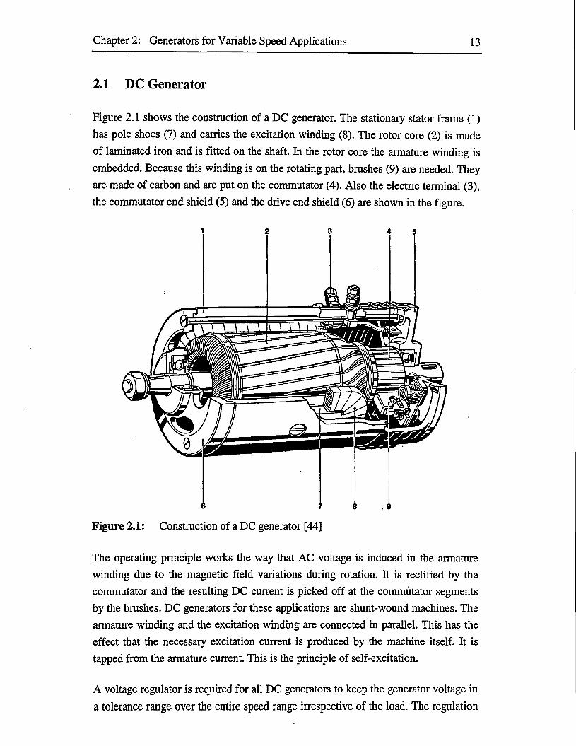
Figure 2.1 shows the construction of a DC generator. The stationary stator frame (1)
has pole shoes (7) and carries the excitation winding (8). The rotor core (2) is made
of laminated iron and is fitted on the shaft. In the rotor core the armature winding is
embedded. Because this winding is on the rotating part, brushes (9) are needed. They
are made of carbon and are put on the commutator (4). Also the electric terminal (3),
the commutator end shield (5) and the drive end shield (6) are shown in the figure.
2 3 5
The operating principle works the way that AC voltage is induced in the armature
winding due to the magnetic field variations during rotation. It is rectified by the
commutator and the resulting DC current is picked off at the commutator segments
by the brushes. DC generators for these applications are shunt-wound machines. The
armature winding and the excitation winding are connected in parallel. This has the
effect that the necessary excitation current is produced by the machine itself. It is
tapped from the armature current. This is the principle of self-excitation.
A voltage regulator is required for all DC generators to keep the generator voltage in
a tolerance range over the entire speed range irrespective of the load. The regulation
Chapter 2: Generators for Variable Speed Applications 14
principle consists of regulating the excitation current as a function of the generated
voltage. The excitation current is regulated by a regulating contact which interrupts
the excitation current when a voltage tolerance range is exceeded and is contacted
again when a minimum set value is reached. This voltage regulator protects the
electric loads against overvoltage and prevents the battery from being overcharged. It
also takes the electro-chemical properties of the battery into account, like the
temperature-depending charging voltage.
Besides a voltage regulator DC generators need an extra current regulator which
protects the machine against overloading. To protect the battery from discharging at
low speeds an independent electromagnetic relay is also required to interrupt the
connection between the generator and the battery.
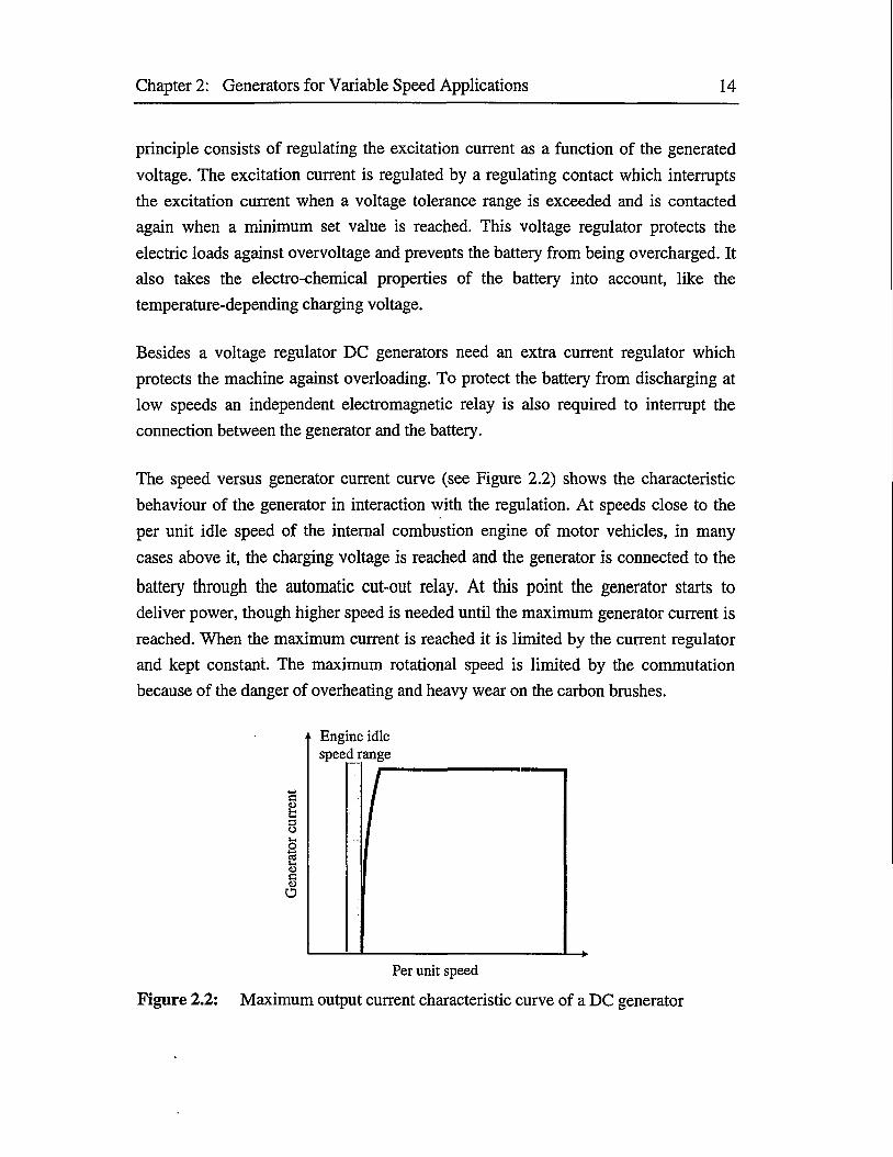
The speed versus generator current curve (see Figure 2.2) shows the characteristic
behaviour of the generator in interaction with the regulation. At speeds close to the
per unit idle speed of the internal combustion engine of motor vehicles, in many
cases above it, the charging voltage is reached and the generator is connected to the
battery through the automatic cut-out relay. At this point the generator starts to deliver power, though higher speed is needed until the maximum generator current is
reached. When the maximum current is reached it is limited by the current regulator
and kept constant. The maximum rotational speed is limited by the commutation
because of the danger of overheating and heavy wear on the carbon brushes.
Engine idle speed range
Per unit speed
Figure 2.2: Maximum output current characteristic curve of a DC generator
Chapter 2: Generators for Variable Speed Applications 15
2.2 Alternator
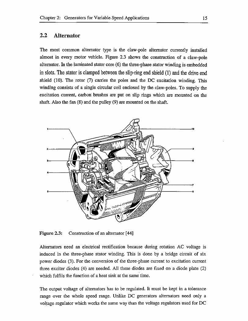
The most common alternator type is the claw-pole alternator currently installed
almost in every motor vehicle. Figure 2.3 shows the construction of a claw-pole
alternator. In the laminated stator core (6) the three-phase stator winding is embedded
in slots. The stator is clamped between the slip-ring end shield (1) and the drive end
shield (10). The rotor (7) carries the poles and the DC excitation winding. This
winding consists of a single circular coil enclosed by the claw-poles. To supply the
excitation current, carbon brushes are put on slip rings which are mounted on the
shaft. Also the fan (8) and the pulley (9) are mounted on the shaft.
Figure 2.3: Construction of an alternator [44]
Alternators need an electrical rectification because during rotation AC voltage is
induced in the three-phase stator winding. This is done by a bridge circuit of six
power diodes (3). For the conversion of the three-phase current to excitation current
three exciter diodes (4) are needed. All these diodes are fixed on a diode plate (2)
which fulfils the function of a heat sink at the same time.
The output voltage of alternators has to be regulated. It must be kept in a tolerance
range over the whole speed range. Unlike DC generators alternators need only a
voltage regulator which works the same way than the voltage regulators used for DC

Chapter 2: Generators for Variable Speed Applications 16
generators. The excitation current is diminished, when the voltage tolerance range is
exceeded and increased again after a minimum set value is reached. The regulator (5)
is connected to the brush holders and, depending on the type, sometimes mounted
straight on them like in figure 2.3.
Generally different types of regulators exist but the latest invented hybrid regulator is
mostly used nowadays. Other regulator types are the conventional electromagnetic
vibrating-type and the transistor regulator. The advantages of the hybrid regulator are
compact construction, high reliability, small amount of components and connections.
The main component of the hybrid regulator is an integrated circuit that combines all
control functions. Basically the hybrid regulator is a further development of the
transistor regulator.
The invention of the transistor regulator was a large progress in regulator technology
because it has no mechanical contacts and moving parts anymore, thus it is
maintenance free. It is also a lot smaller and lighter than the conventional
electromagnetic vibrating-type regulator and insensitive to vibrations. These
advantages allow the transistor regulator to be mounted directly on the alternator.
Other positive features are short switching times, narrow regulation tolerances,
allowance of high switching currents, spark-free switching and electronic
temperature compensation. The conventional electromagnetic vibrating-type
regulator is not used anymore because of the obvious advantages of the new regulator
types.
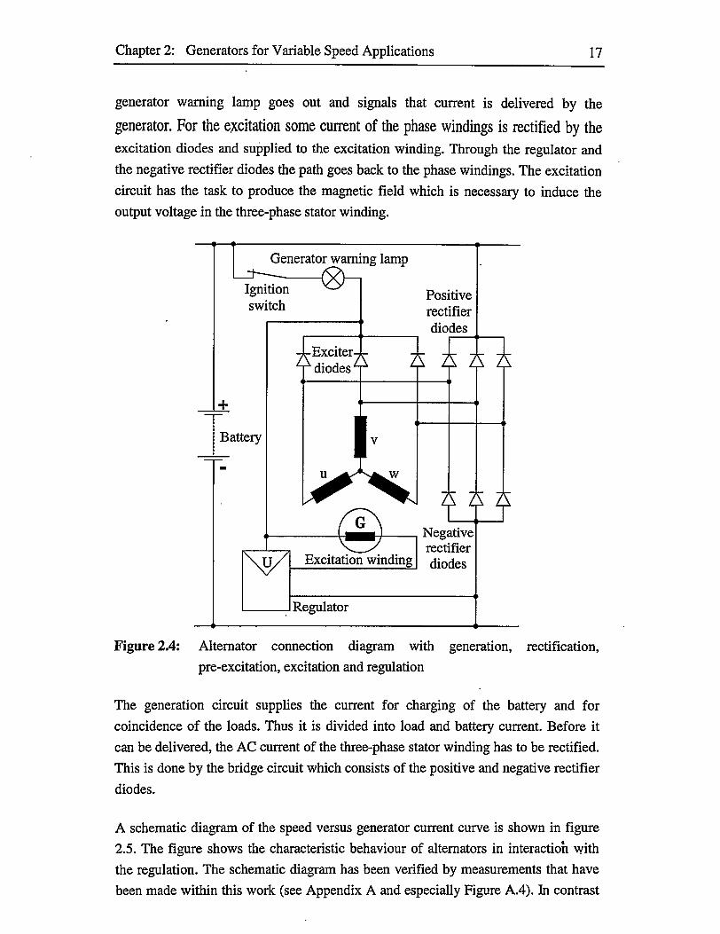
Figure 2.4 shows the total connection diagram for an alternator with generation,
rectification, pre-excitation, excitation and regulation. The interaction of the three
generator circuits for pre-excitation, excitation and generation can be seen. The
pre-excitation starts when the ignition is switched on and the excitation current
supplied by the battery flows through the generator warning lamp to the excitation
winding of the rotor. From there it flows through the regulator to ground. The
pre-excitation is necessary because at low speeds the remanence in the iron core is
not sufficient to build up a magnetic field just by a self-excitation strong enough to
generate the desired minimum voltage for the excitation circuit. At least the
generated voltage has to be higher than the voltage drop of the in series connected
negative rectifier diode and excitation diode.
When the desired minimum voltage is reached, the excitation circuit starts to work
and the excitation is taken straight from the generated current. No external power
source is needed after that. The alternator excites itself. At the same time the
Chapter 2: Generators for Variable Speed Applications 17
generator warning lamp goes out and signals that current is delivered by the
generator. For the excitation some current of the phase windings is rectified by the
excitation diodes and supplied to the excitation winding. Through the regulator and
the negative rectifier diodes the path goes back to the phase windings. The excitation
circuit has the task to produce the magnetic field which is necessary to induce the
output voltage in the three-phase stator winding.
Generator warning lamp
Ignitionswitch
Positiverectifierdiodes
Exciterdiodes'
Battery
NegativerectifierdiodesExcitation winding
Regulator
Figure 2.4: Alternator connection diagram with generation, rectification,
pre-excitation, excitation and regulation
The generation circuit supplies the current for charging of the battery and for
coincidence of the loads. Thus it is divided into load and battery current. Before it
can be delivered, the AC current of the three-phase stator winding has to be rectified.
This is done by the bridge circuit which consists of the positive and negative rectifier
diodes.
A schematic diagram of the speed versus generator current curve is shown in figure
2.5. The figure shows the characteristic behaviour of alternators in interaction with
the regulation. The schematic diagram has been verified by measurements that have
been made within this work (see Appendix A and especially Figure A.4). In contrast

Chapter 2: Generators for Variable Speed Applications 18
to DC generators alternators already deliver an output current at the per unit idle
speed of the internal combustion engine of motor vehicles. This has the advantage
that the battery can be kept in a good state of charge even in winter and while driving
in town with frequent waiting times. The output current at idle speed reaches
approximately one third of the absolute maximum output current.
Engine idlespeedrange
Per unit speed
Figure 2.5: Maximum output current characteristic curve of an alternator
The maximum output current increases rapidly with an increase of the speed at low
speeds. At high speeds it increases slightly with an increase of speed. It is not kept
constant like for DC generators because alternators are not equipped with current
regulation. Compared with DC generators the reached maximum output current is
always higher. The maximum rotational speed is limited by centrifugal force and
appearing vibrations.
2.3 Weak Spots of Existing Technology
As already mentioned, DC generators were used at first for low output power and
variable speed applications but nowadays they are almost not used anymore. The
main reason for this can be seen from the maximum output current characteristic
curve which was already shown in figure 2.2. It can be seen that the speed range is
severely restricted to a range not broad enough for modem variable speed
applications. Especially for motor vehicles the output characteristic does not meet the
demands because no energy is supplied at the per unit idle speed. This will cause a
discharge of the battery while driving in town because of the high average proportion
of waiting times in town driving. The development of the average proportion of

Chapter 2: Generators for Variable Speed Applications 19
waiting times in town driving from 1950 to 1990 is illustrated in figure 2.6 and it can
be observed that the situation has not become better.
Figure 2.6: Development of average proportion of waiting times in town driving from 1950 to 1990
Another disadvantage of DC generators is the need of maintenance due to the wear of
the carbon commutator brushes. A high output power can be reached only with large
dimensions and high weight. The advantage and the reason for former use is the
simple, mechanical rectification by the commutator. Since semiconductor
components are common and inexpensive, the mechanical rectification is not needed
or advantageous anymore. Rectification can be better and easier made by bridge
circuits of power diodes.
Nowadays the alternator is used for low output power and variable speed
applications. It has some advantages compared with DC generators. Especially the
maximum output current characteristic curve (already shown in figure 2.5) is more suitable. The alternator supplies energy over a broader speed range and even at the
per unit idle speed of the combustion engine of motor vehicles. Also the output
power is higher and that is important because the demand of output power has increased. Figure 2.7 shows the rapid increase of the required generator output for
motor vehicles since 1950.
Another advantage of alternators is the electronic rectification of the three-phase
current with diodes, because it makes the mechanical rectification by the commutator
superfluous. This, together with the fact that the rotor winding is only for the
excitation, decreases the wear of the brushes because the coal of the brushes will be

Chapter 2: Generators for Variable Speed Applications 20
rubbed off more slowly and because the excitation current is a lot smaller than the
output current. This guarantees a longer service life. Mostly the brushes or the
bearings wear out first after around 100,000 km. The diodes perform also an
automatic relay which cuts the alternator from the battery if the alternator voltage
drops below the battery voltage. Alternators are also lighter than DC generators and
they can better tolerate external influences like high temperatures, damp, dirt and
vibrations. The disadvantage of alternators is their smaller efficiency.
1200 T
1000 --
800 --
Figure 2.7: Development of generator output from 1950 to 1990
As just pointed out alternators have some advantages compared with DC generators,
but still they have their weak spots. One main disadvantage is that they provide only
approximately one third of the maximum output power at idle speed (see Chapter
2.2). This can cause the discharging of the battery under unfavourable conditions, for
example in winter time when many loads are switched on and long waiting times
occur at the same time.
The other main disadvantage of alternators is the low efficiency. Especially at high
speeds the efficiency decreases noticeably. This can be seen from the measurement
results documented in the Appendix A. Figure A.5 shows the decrease of efficiency
with increasing speed. In the same picture it can also be seen that the efficiency
decreases with a decrease of the load. Alternators reach a reasonable efficiency only
at nominal output power and not too high speed. The low alternator efficiency reacts,
for example negatively on the fuel consumption of motor vehicles, as it is
investigated in reference [25].

Chapter 2: Generators for Variable Speed Applications 21
The constantly increasing power demand and the changed traffic conditions led to
such requirements that the DC generator was not capable of fulfilling them anymore.
The alternator solved the problems that cropped up with the new demands.
Nowadays the development is going still in the direction that higher and higher
electric power is demanded. It can be noticed that the alternators are almost reaching
their output power limits and new technology or different system suppositions, like a
higher voltage level, are necessary to fulfil the requirements of modem car
technology. Switched reluctance generators can exceed the alternator limits, and they
have also other advantages.
2.4 Supposed Improvements and Advantages of Switched
Reluctance Technology
Comparisons of switched reluctance machines with other machine types have been
made and they are reported in literature [5],[15],[28],[35],[47]. Most of them are
concentrating on motor applications and are quite general, but some of them also
point out that the advantages of switched reluctance machines can be recognised in
all four quadrants of operation (see Figure 3.1).
The first main advantage of switched reluctance generators is the high output power.
A higher output power compared with other machine types is reached because more
copper can be fitted in the large slot area. Over a broad speed range and especially at
low speeds the output power is higher than for alternators. Only at very high speeds it
is lower. The maximum output power is supplied over a broad range at medium
speeds.
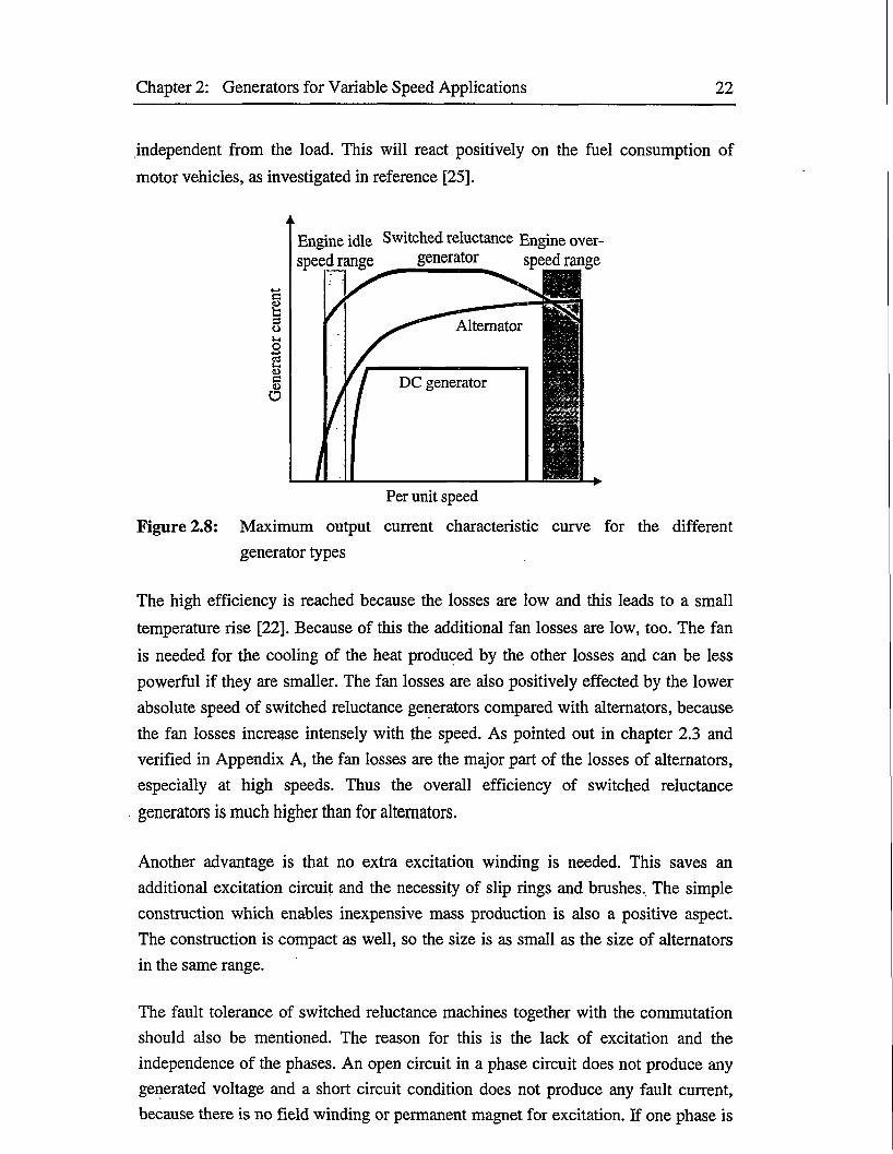
Figure 2.8 shows a schematic comparison of the maximum output current of the three
generator types versus the per unit speed range of the internal combustion engine of a
motor vehicle. It can be seen in the figure that compared with the alternator the
maximum output current of switched reluctance generators is around three times
higher at idle speed and still higher until the motor overspeed range is reached. In the
overspeed range it is smaller, but this speed range is rarely used for driving. The
output current behaviour is almost equal to the output power behaviour because of
the nearly constant average voltage.
The other main benefit of switched reluctance generators is the high efficiency.
Contrarily to alternators, it is almost constant over the whole speed range and nearly
Chapter 2: Generators for Variable Speed Applications 22
independent from the load. This will react positively on the fuel consumption of
motor vehicles, as investigated in reference [25].
Engine idle Switched reluctance Engine overspeed range generator speed range
Alternator
DC generator
Per unit speed
Figure 2.8: Maximum output current characteristic curve for the different
generator types
The high efficiency is reached because the losses are low and this leads to a small
temperature rise [22]. Because of this the additional fan losses are low, too. The fan
is needed for the cooling of the heat produced by the other losses and can be less
powerful if they are smaller. The fan losses are also positively effected by the lower
absolute speed of switched reluctance generators compared with alternators, because
the fan losses increase intensely with the speed. As pointed out in chapter 2.3 and
verified in Appendix A, the fan losses are the major part of the losses of alternators,
especially at high speeds. Thus the overall efficiency of switched reluctance
generators is much higher than for alternators.
Another advantage is that no extra excitation winding is needed. This saves an
additional excitation circuit and the necessity of slip rings and brushes. The simple
construction which enables inexpensive mass production is also a positive aspect.
The construction is compact as well, so the size is as small as the size of alternators
in the same range.
The fault tolerance of switched reluctance machines together with the commutation
should also be mentioned. The reason for this is the lack of excitation and the
independence of the phases. An open circuit in a phase circuit does not produce any
generated voltage and a short circuit condition does not produce any fault current,
because there is no field winding or permanent magnet for excitation. If one phase is

Chapter 2: Generators for Variable Speed Applications 23
faulted, the healthy ones can operate almost unaffected because of the independence
of the phases. Commutation units of the form of the classic converter (see chapter
3.3.1) have no shoot-through path and thus the DC supply can be shorted only if the
phase winding itself is short circuited. Additional information on the behaviour of
switched reluctance machines under internal and external fault conditions is given in
the references [1],[2],[26].
The disadvantages of switched reluctance generators are the high level of current
ripple and the control dependent on rotor position, which requires a rotor position
feedback. They are also known for producing higher acoustic noise [51]. The main
advantages of high output power and high efficiency compensate these
disadvantages.

24
3 Principle and Theory of Switched Reluctance Generators
Switched reluctance machines are widely used for motor applications and because of
this most of the published theory is about motoring operation. Only a bit of
information on switched reluctance generators can be extracted from the literature.
On the other hand motoring and generating are operating states of one machine. This
is the reason why motor theory and generator theory are connected. Figure 3.1
illustrates the four quadrant operation of a machine. The theory mentioned in this
chapter refers to literature, if mentioned, or is verified by investigations with the
simulation tool PC-SRD [30],[31]. This chapter gives an overview of the switched
reluctance machine theory with special attention to the characteristics of generating
operation.
Forward
r<ov> 0
Generating
T> 0 v > 0
Motoring
Motoring0
GeneratingT< 0 T> 0v<0 v< 0
Reversei
Figure 3.1: Speed over torque diagram for four quadrant machine operation
3.1 Construction
The main construction characteristic of switched reluctance machines is that they
have salient stator and rotor poles which differ in number. Basically the motion can
be rotary or linear and the rotor interior or exterior, but interior rotors with rotary
motion are most common. The way of motion and the arrangement of the rotor
determine the cross section layout. Only the most commonly used construction is
described here. Another basic characteristic is that only the stator poles are equipped
with windings and the rotor carries no windings. Usually the windings of two
opposite poles form one phase winding. Both the rotor and the stator are made of

Chapter 3: Principle and Theory of Switched Reluctance Generators 25
laminated iron. Figure 3.2 shows the cross section of a three phase 6/4-switched
reluctance machine to give a first impression of the construction.
Figure 3.2: Cross section of a three phase 6/4-switched reluctance machine
3.1.1 Basic Characteristics
Switched reluctance machines can be distinguished by the number of phases m, stator
Nt and rotor poles Nt. Different combinations of these main design criteria enable afunctional machine. It must be mentioned that the one and two phase machines need
assistance for starting if they are used for motor applications. Table 3.1 shows
different possible phase and pole combinations most commonly used in practice [27].
The combinations supported by the PC-SRD can be seen in reference [30].
All combinations included in the table are so called regular designs. A regular design
means that the stator and rotor poles are symmetric about their centre lines and
equally spaced around the rotor and stator respectively. Most of the practical
switched reluctance machine designs are included in the table, but irregular machines
are existing, too, as it can be seen in reference [27]. This reference also gives an
overview of different motor designs. The stroke angle e = 360°/(mA/r) and the number
of strokes per revolution Mtrokes/rev = rnNr can be calculated from the number of
phases and rotor poles. These characteristic values are also included in the table.

Chapter 3: Principle and Theory of Switched Reluctance Generators 26
Table 3.1: Phase and pole combinations
Number of Phasesm
Number of Stator Poles
Ns
Number of Rotor Poles Nt
Number of Working Poles
per Phase p
Stroke Angle£
Strokes per RevolutionN .strokes/rev
1 2 2 1 180.00 22 4 2 1 90.00 42 8 4 2 45.00 83 6 2 1 60.00 63 6 4 1 30.00 123 12 8 2 15.00 243 18 12 3 10.00 363 24 16 4 7.50 484 8 6 1 15.00 244 16 12 2 7.50 485 10 4 1 18.00 205 10 6 1 12.00 305 10 8 1 9.00 406 12 10 1 6.00 606 24 20 2 3.00 1206 12 14 1 4.29 847 14 10 1 5.14 707 14 12 1 4.29 84
Other characteristics of a switched reluctance machine are the absolute and effective
torque zones and the absolute and effective overlap ratios. The absolute torque zone
is the angle through which one phase can produce a non-zero torque in motoring
operation. For a regular motor it is maximally 180°/Nt. In generating operation this is
the maximum zone where a positive output current is available. In this operating
mode a better name would be absolute current zone. The effective value of this
dimension is comparable to the smaller pole arc of the overlapping rotor and stator
poles and it gives the angle where useful torque or respectively useful output current
can be produced.
The absolute overlap ratio is defined as the ratio of the absolute torque zone to the
stroke angle. Its value is equal to mil. For a regular motor a value of at least one is
necessary so that torque can be produced at all rotor positions, but a value of one is
not sufficient because the nominal torque can never be provided throughout the
whole absolute torque zone by only one phase. For a generator the same feature can
be seen for the output current.
The effective overlap ratio is defined by the ratio of the effective torque zone and
the stroke angle respectively. It is always smaller than the value of the absolute
overlap ratio. The ratio is approximately equal to the stator pole arc divided by the

Chapter 3: Principle and Theory of Switched Reluctance Generators 27
stroke angle if the stator pole arc is smaller than the rotor pole arc for a regular
machine, which is normal in common conditions. A value of at least one is necessary
to get a starting torque at every rotor position but not sufficient for avoiding torque
ripple. In generating operation there is no need for a starting torque, because it is
given by the driving machine. For a steady output current a value bigger than one of
the effective overlap ratio is necessary.
3.1.2 Envelope and Internal Dimensions
The internal and envelope dimensions mainly determine the machine performance.
The envelope dimensions are the stator lamination diameter A and the overall length
Le which is measured over the end turn overhangs of the winding. These dimensions
define the gross electromagnetic volume Vgross- The net electromagnetic volume Vnet
is defined by the stack length Lstk and the stator lamination diameter. The stack length
is an inner dimension and the overall length can be calculated from it by
Le=Lstk+ 2 L0h with L0h as the overhang length of the winding. The overhang length
is approximately equal to the stator pole width ts which is introduced later in this
chapter. All these and some more inner dimensions (stator slot bottom diameter Ab,
shaft diameter Ah, minor rotor diameter Am, rotor diameter A and air gap length 8) are illustrated in figure 3.3. The figure shows the longitudinal cross section of a
machine and the main parts of the construction are named.
Some ratios of the above mentioned dimensions can be used for machine
characterisation. One is the standard or split ratio which is defined by the rotor
diameter divided by the stator diameter. Dc/Ds can vary between 0.4 and 0.7 but for
most designs it is between 0.5 and 0.55 [27] and tends to be larger with a higher
number of poles. According to the reference [10] a suitable value should be between
0.57 and 0.63. Another characterising ratio is the length per diameter ratio given' exactly by the stack length and the rotor diameter. A typical value for Atk/A is 1.
From the net electromagnetic rotor volume and the torque T the torque per unit rotor
volume rpURv can be estimated as
^puRV —f D“4k
(3.1)
According to table 3.2 the Tpurv value enables a rough categorisation of the machine
and shows the extent of machine utilisation which is mostly limited by the used

Chapter 3: Principle and Theory of Switched Reluctance Generators 28
cooling method. Usually this value is used as a starting point for the first rough
estimation of a new machine design.
Stator
Stator pole
Rotor
Rotor pole
End turn overhang
Winding
Stator yoke
Figure 3.3: Longitudinal machine cross section (rotor in aligned position)
Other inner dimensions can be seen from the cross-section of a machine. Figure 3.4
shows the cross section of a three phase 6/4-machine, including the inner dimensions
shaft radius Rsh, minor rotor radius Rq, rotor radius Ru radius of stator slot bottom R2. stator outside radius Rz, rotor pole arc /Jr, stator pole arc /5S, rotor pole width /, and
stator pole width ts.
Table 3.2: Machine categorisation from the torque per unit rotor volume [ 27 j
Machine category T durv in kNm/m3Small totally enclosed machines 2.5-7Integral-kW industrial machines 7-30High-performance servomotors 15-50Aerospace machines 30-75Large liquid-cooled machines 100 - 250
All important information of a machine construction is given with the mentioned
basic dimensions and all other necessary values can be calculated from them, like the rotor tooth width
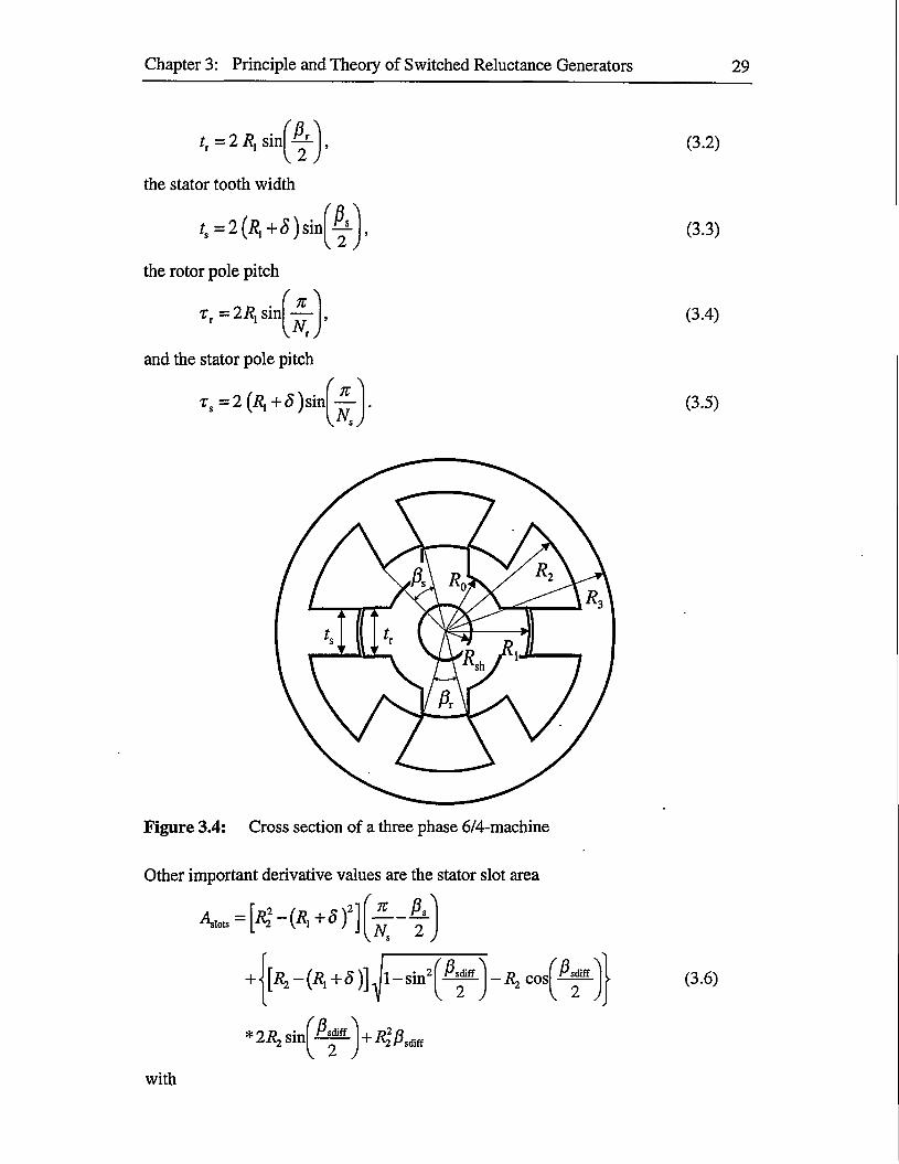
Chapter 3: Principle and Theory of Switched Reluctance Generators 29
tt=2Rx sin^L
the stator tooth width
K -2(^i+<$)sin^-^
the rotor pole pitch
KTr = 2ft, sin
and the stator pole pitch
ts = 2 (ft, +5 )sin
Other important derivative values are the stator slot area
Aio*-[%ARi+sT]{y-Y
+ [ft, - (R, + 5)] ^jl - sin' Psdiff D Pstiff~ ft; COS
(3.2)
(3.3)
(3.4)
(3.5)
(3.6)
with
2

Chapter 3: Principle and Theory of Switched Reluctance Generators 30
where the winding is embedded, the stator iron volume
v,„ = {* [*? - ft+S f ] ■- WA-} (3.7)
and the rotor iron volume
(3.8)
with Asiotr as the rotor slot area which is calculated in the same way than the stator
slot area, but the values R2, (Ri+S), Ns and j3s have to be replaced by Ru Ro, Nr and jSr
and the within used abbreviation f3sm then changed to /Wf respectively.
Also some derivative dimensions can be defined. Mainly the rotor slot depth
dT = Rx-Rq, the stator slot depth ds = R2-(R\+S), the rotor yoke thickness yT = Ro-Rsh and the stator yoke thickness ys = R3-R2 are important to mention and they are
especially used during the designing process because of their better clarity in
connection to the electric and magnetic phenomena occurring in a machine.
3.1.3 Pole Geometry
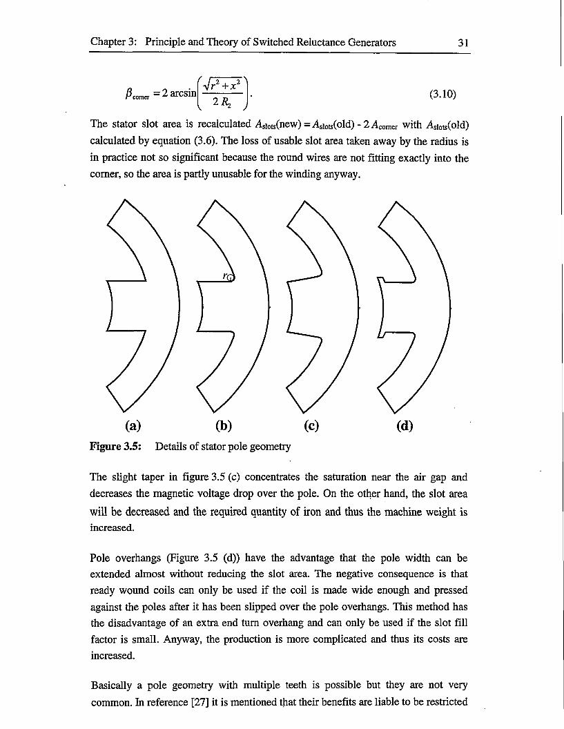
Figure 3.4 has already shown the basic pole geometry, but variations especially for
the stator poles are common and sometimes advantageous depending on the
intention. Figure 3.5 shows some different possible modifications of the stator pole
geometry. Modifications of the rotor pole geometry are not so common and, because
of that, not mentioned here.
One very useful and advantageous modification of the standard pole geometry
(Figure 3.5 (a)) is shown in figure 3.5 (b). The radius at the comers of the slot bottom
increases the stiffness of the poles against lateral deflection and also stabilises the
stator. This has a positive effect on acoustic noise reduction, but on the other hand
the usable slot area for embedding of the winding is decreased. The comer area taken
by the radius r is
A,'comercomerasa.-------COS2 2 1 (3.9)
with
and
Chapter 3: Principle and Theory of Switched Reluctance Generators 31
^corner = 2 arcscomer (3.10)
The stator slot area is recalculated Asiots(new) = Asi0ts(old) - 2 Acomer with Asi0ts(old)
calculated by equation (3.6). The loss of usable slot area taken away by the radius is
in practice not so significant because the round wires are not fitting exactly into the
comer, so the area is partly unusable for the winding anyway.
(a) (C)(b) (d)
Figure 3.5: Details of stator pole geometry
The slight taper in figure 3.5 (c) concentrates the saturation near the air gap and
decreases the magnetic voltage drop over the pole. On the other hand, the slot area
will be decreased and the required quantity of iron and thus the machine weight is
increased.
Pole overhangs (Figure 3.5 (d)) have the advantage that the pole width can be
extended almost without reducing the slot area. The negative consequence is that
ready wound coils can only be used if the coil is made wide enough and pressed
against the poles after it has been slipped over the pole overhangs. This method has
the disadvantage of an extra end turn overhang and can only be used if the slot fill
factor is small. Anyway, the production is more complicated and thus its costs are
increased.
Basically a pole geometry with multiple teeth is possible but they are not very
common. In reference [27] it is mentioned that their benefits are liable to be restricted
Chapter 3: Principle and Theory of Switched Reluctance Generators 32
to low speeds and they have the same disadvantage concerning the winding than a
pole geometry with overhangs as well.
3.1.4 Windings
The windings of switched reluctance machines are simpler than those of other machine types and an extra winding for excitation is not needed. Only one coil is
wound on each stator pole and it is not necessary to make use of special winding
patterns. Normally the windings of opposite poles comprise to one phase. They can
be connected in series or in parallel.
Basically the winding can be defined by the slot fill factor Sen, the number of turns
per pole Np and the number of parallel paths per phase /Vpath. The theoretical
maximum achievable slot fill factor is restricted to itlA because round wires can not
be joined to each other without leaving some empty space in-between. In practice the
theoretical slot fill factor can not be reached because of the area losses by the
insulation, the distance that has to be kept from the air gap and the geometrical
circumstances. A realistic maximum slot fill factor for an insulated slot area is
between 0.6 and 0.7.
The slot fill factor also determines if pre-wound windings can be used. In that case
the slot fill factor should be smaller than around 0.4. This value ensures that the
ready wound winding can be slipped over the poles. It has to be also permissible by
the pole geometry (see chapter 3.1.3).
3.2 Working Principle
The working principle of switched reluctance machines is based on the change of the
magnetic reluctance depending on the rotor position. The rotor tries to adjust the
position with the smallest magnetic reluctance and produces a torque. For a generator
with a torque given by a driving machine, a voltage which will cause a current will be
induced in the stator winding. Because the rotor poles are without a winding, the
excitation and the output current must be taken from the same winding. Thus the
current of each phase has to be switched depending on the rotor position.

Chapter 3: Principle and Theory of Switched Reluctance Generators 33
3.2.1 Rotor Position Dependency
As already mentioned, the working principle is based on the rotor position. To
describe this dependency it is easier and enough to concentrate just on the positions
according to one phase. Then two positions and two zones can be distinguished. The
positions are the aligned and the unaligned position.
The rotor is in the aligned position according to one phase when one pair of the rotor
poles is exactly aligned with the stator poles on which the winding of this phase is
wound. Figure 3.6 illustrates the aligned position on the phase in the horizontal axis
for a 6/4-switched reluctance machine.
Figure 3.6: 6/4-switched reluctance machine in the aligned position on the phasewhich is marked
In this position the magnetic reluctance of the flux path is lowest because most of the
reluctance is in the air gap and the gap is smallest in this position. Because the
reluctance is at its minimum, the phase inductance is at its maximum. The reluctance
in the iron is lower than in the air gap but can not be neglected, because the long path
through the iron also absorbs a significant magneto motive force. The iron is also
susceptible to saturation, especially in the stator and rotor yokes. Because of these
reasons the aligned inductance will be reduced.
The aligned position is a stable position. A current in this phase can not produce a
torque because the magnetic reluctance is already at its minimum. If the rotor is
displaced to either side, a restoring torque tends to return the rotor towards the
position of minimum reluctance - the aligned position.
Chapter 3: Principle and Theory of Switched Reluctance Generators 34
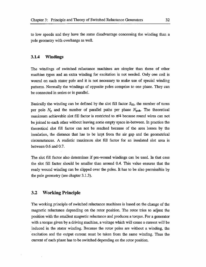
The rotor is in the unaligned position according to one phase when the interpolar axis
of the rotor is aligned with the stator poles on which the winding of this phase is
wound. Figure 3.7 illustrates the unaligned position on the horizontal axis for the
same 6/4-switched reluctance machine.
Figure 3.7: 6/4-switched reluctance machine in the unaligned position on the
phase which is marked
In this position the magnetic reluctance is at its highest because of the large air gap.
Because the reluctance is at its maximum, the phase inductance is at its minimum. The iron is unreceptive to saturation in this position because the current when
saturation begins has to be much higher than in the aligned position. This is because
the leakage flux is relatively much greater and the winding is laid out to avoid high
saturation even in the aligned position.
If the phase is excited, the unaligned position is an unstable equilibrium. There is no
torque in this position, but if the rotor is displaced to either side, a torque appears that
tends to displace the rotor further until it is aligned with the next aligned position.
The intermediate positions can be summarised to two zones. The direction of forward
motion is always set counterclockwise. Then the intermediate positions of the first
zone are those that are taken while the rotor turns from the unaligned towards the
aligned position. Respectively, when the rotor turns from the aligned towards the
following unaligned position, the intermediate positions of the second zone are taken.
Figure 3.8 shows these two zones for the same 6/4-switched reluctance machine.

Chapter 3: Principle and Theory of Switched Reluctance Generators 35
In the first zone the magnetic reluctance decreases towards the aligned position, thus
the inductance increases. Especially with the start of pole overlap the inductance
changes rapidly because of the smaller air gap. Before overlap there is only a slight
increase. In the second zone the inductance shows a contrary behaviour. It decreases
with further rotation. With the start of pole overlap also the iron starts to be
susceptible to saturation. Before the pole overlap there is only the possibility of local
saturation of the pole comers.
direction ofrotation
unaligned
Zone 2
aligned
Zone 1
unaligned
Figure 3.8: 6/4-switched reluctance machine with the two zones of intermediate
rotor positions
If the phase is excited in the first zone, the appearing torque assists the
counterclockwise rotation towards the aligned position. Thus this zone is relevant forthe motoring operation. In the second zone the appearing torque counteracts against the counterclockwise rotation and a driving torque is necessary to enable the
movement towards the unaligned position. Thus this zone is relevant for generating
operation.
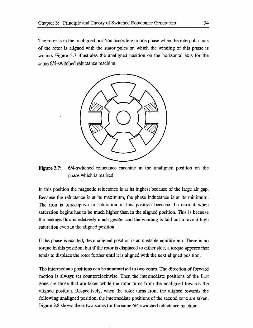
The influence of the different rotor positions can be also described by the
magnetisation and inductance curves. These figures give a closer survey and form the
basis for the further mathematical description. Figure 3.9 shows a set of
magnetisation curves. The flux linkage y/ versus the current i is presented for one
phase.
Chapter 3: Principle and Theory of Switched Reluctance Generators 36
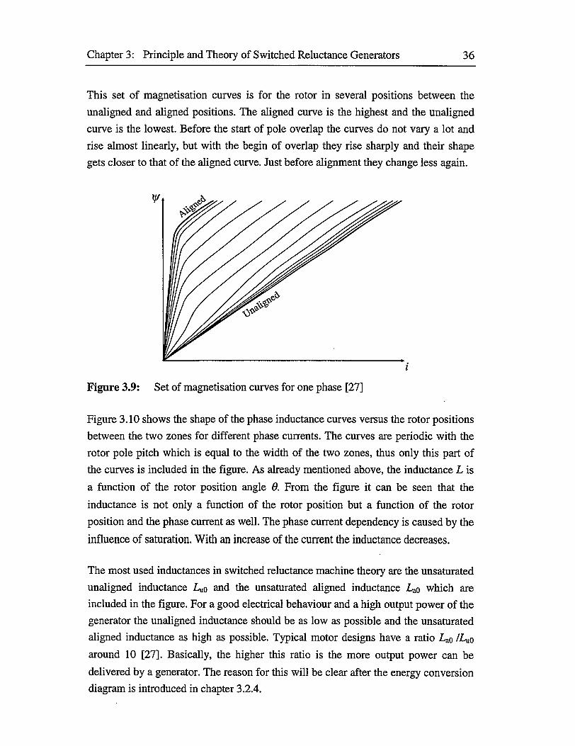
This set of magnetisation curves is for the rotor in several positions between the
unaligned and aligned positions. The aligned curve is the highest and the unaligned
curve is the lowest. Before the start of pole overlap the curves do not vary a lot and
rise almost linearly, but with the begin of overlap they rise sharply and their shape
gets closer to that of the aligned curve. Just before alignment they change less again.
V
i
Figure 3.9: Set of magnetisation curves for one phase [27]
Figure 3.10 shows the shape of the phase inductance curves versus the rotor positions
between the two zones for different phase currents. The curves are periodic with the
rotor pole pitch which is equal to the width of the two zones, thus only this part of
the curves is included in the figure. As already mentioned above, the inductance L is
a function of the rotor position angle G. From the figure it can be seen that the
inductance is not only a function of the rotor position but a function of the rotor
position and the phase current as well. The phase current dependency is caused by the
influence of saturation. With an increase of the current the inductance decreases.
The most used inductances in switched reluctance machine theory are the unsaturated
unaligned inductance Lu0 and the unsaturated aligned inductance Lao which are
included in the figure. For a good electrical behaviour and a high output power of the
generator the unaligned inductance should be as low as possible and the unsaturated
aligned inductance as high as possible. Typical motor designs have a ratio Lao /Luo
around 10 [27]. Basically, the higher this ratio is the more output power can be
delivered by a generator. The reason for this will be clear after the energy conversion
diagram is introduced in chapter 3.2.4.
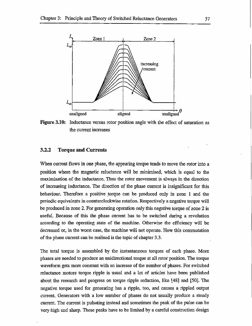
Chapter 3: Principle and Theory of Switched Reluctance Generators 37
Zone 1 Zone 2
increasing/current
unaligned aligned unaligned
Figure 3.10: Inductance versus rotor position angle with the effect of saturation as
the current increases
3.2.2 Torque and Currents
When current flows in one phase, the appearing torque tends to move the rotor into a
position where the magnetic reluctance will be minimised, which is equal to the maximisation of the inductance. Thus the rotor movement is always in the direction
of increasing inductance. The direction of the phase current is insignificant for this
behaviour. Therefore a positive torque can be produced only in zone 1 and the
periodic equivalents in counterclockwise rotation. Respectively a negative torque will
be produced in zone 2. For generating operation only this negative torque of zone 2 is
useful. Because of this the phase current has to be switched during a revolution
according to the operating state of the machine. Otherwise the efficiency will be
decreased or, in the worst case, the machine will not operate. How this commutation
of the phase current can be realised is the topic of chapter 3.3.
The total torque is assembled by the instantaneous torques of each phase. More
phases are needed to produce an unidirectional torque at all rotor position. The torque
waveform gets more constant with an increase of the number of phases. For switched
reluctance motors torque ripple is usual and a lot of articles have been published
about the research and progress on torque ripple reduction, like [48] and [50]. The
negative torque used for generating has a ripple, too, and causes a rippled output
current. Generators with a low number of phases do not usually produce a steady
current. The current is pulsating instead and sometimes the peak of the pulse can be
very high and sharp. These peaks have to be limited by a careful construction design

Chapter 3: Principle and Theory of Switched Reluctance Generators 38
and by a suitable control strategy (see chapter 3.5). Otherwise the commutation
devices might be destroyed.
Figure 3.11 shows the output current waveform for a 6/4-switched reluctance
generator with 12 V supply voltage and 1.5 kW output power at a speed of 3,000 rpm
computed by the simulation tool PC-SRD. It can be seen that the positive current
peak is quite sharp. This is because the excitation is taken straight from the output current in the beginning and only later from the supply. The negative part of the
waveform is wider and the peak is a lot higher, so a high output is reached.
PC Link curr» r>~A x 1.0*2
Peter position x 1.0*1
Figure 3.11: DC link current versus rotor position for a 6/4-switched reluctance
generator with 12 V supply voltage and 1.5 kW output power at a
speed of 3,000 rpm
The necessary input torque for generation of the DC link current in figure 3.11 is
shown in figure 3.12. This torque has to be provided by the driving machine. From
the figure it can be seen that also the input torque has very high peaks like the
generated output current.
Torque versus rotor positionie < Nm > x l.Oel
12.00 18.00-0.25--0.50--0.75--1.00-
-1.25--1.50-
Rotor position < deq ) x l.Oel
Figure 3.12: Torque versus rotor position for a 6/4-switched reluctance generator
with 12 V supply voltage and 1.5 kW output power at 3,000 rpm

Chapter 3: Principle and Theory of Switched Reluctance Generators 39
3.2.3 Mathematical Description
The mathematical description of the switched reluctance machine is based on the
voltage equation and the energy balance. The equations are derived for an one-phase
model with neglecting skin and hysteresis effects and magnetic coupling of the
phases. The voltage equation of one phase is
u = Ri+M$. (3.11)at
with the phase resistance R, the phase current i and the phase flux linkage iff. The flux
linkage depends on the phase current and rotor position angle d which are changing
with time. The power balance
ui = Ri2 + i dif/ di . diff dd■+i (3.12)
di dt dd dtis got by multiplying the voltage equation with the phase current. The used energy
ui dt — R ?dt+i ^ di+i ^ dd — R i2dt+dWt + dWm (3.13)
consists of the change in mechanical work dWm,. stored field energy dW{ and
resistance losses. The magnetical energy depends on the current and the rotor
position and its change is given by
dWf=^di+^-dd.f di dd
Thus the change of the mechanical energy is
(3.14)
(3.15)
The energy stored in the magnetic field at a certain operative condition can be calculated by
W(=ji diff =iy/-j\]/di, (3.16)
(3.17)
and its partial derivation regarding the current is
di di l di di
Equation (3.15) has given the change of mechanical energy and it can be written
easier by using equation (3.17). It equals then
(3.18)
The torque equals the derivation of the mechanical energy regarding the rotor
position and it is

Chapter 3: Principle and Theory of Switched Reluctance Generators 40
dWm ,d y dW{ do de de
(3.19)
This equation can be simplified more by replacing the stored field energy with the
coenergy defined by/
W‘=\\}fdi. (3.20)o
The graphic definition of the coenergy is shown by figure 3.13. Also the graphic
interpretation of the stored field energy is given in the figure. The knowledge of the
different energy types is needed for understanding the energy conversion principle
(Chapter 3.2.4).
The flux linkage for the coenergy calculation is
y/ = j(Us-Ri)dt (3.21)
with Us as the supply voltage.
From the figure can be seen straight that the sum of the stored field energy and
coenergy is
Wf+W*=z>. (3.22)
The derivation of the coenergy regarding the rotor position is
dW* = . dyr dW{ dQ dG d6
(3.23)
By replacing this result in equation (3.19) the torque produced by one phase can be
calculated from

Chapter 3: Principle and Theory of Switched Reluctance Generators 41
rM)=Mi=const
(3.24)
The equations (3.20), (3.21) and (3.24) are the general expressions used for switched
reluctance machine calculations. For the realisation of machine designs these
equations have to be solved, but an analytical solution can be found only if the effects
of saturation are neglected. With neglecting the saturation the magnetisation curves
become linear and the instantaneous torque is then
T 1 .2 dL2 dO
(3.25)
For a good machine design the effect of saturation can not be neglected and the
equations (3.20), (3.21) and (3.24) have to be solved. This requires computer-based
simulation because the torque is a function of phase current and rotor position and
affected by saturation, especially intensely at the pole comers. Another reason is that
the instantaneous torque and current vary with the rotor position. Thus the average
torque can be determined only by integration over a period of rotation. Different
computer-based simulation tools or models are reported in literature which are based
on those equations. The already mentioned simulation tool PC-SRD is among them
[6],[29],[31],[32],[33],[41].
3.2.4 Energy Conversion
The energy conversion principle can be best explained by using the energy
conversion diagram which is also called i-yr diagram. An advantage of this diagram
is that the average torque can be derived from the areas on the diagram. This method
for deriving the average torque is used for computer based simulations, for example
the simulation tool PC-SRD uses it [29]. Figure 3.14 shows a diagram like that
computed by the PC-SRD.
Some suppositions have to be set so that the energy conversion diagram can be used.
The machine must rotate at constant speed and a constant voltage has to be supplied
to one phase. For the here described generating operation the voltage is supplied
close before the rotor reaches the aligned position and the commutation takes place
after the aligned position, but before the next unaligned position. The working
principle is explained neglecting all losses for an easier understanding. Thus in the
fundamental figures of the energy conversion diagram (Figure 3.15 to 3.17) which
are used for explanation of the principle, the losses are neglected, too.

Chapter 3: Principle and Theory of Switched Reluctance Generators 42
The energy conversion diagram can be separated into two periods. The first period is
the excitation period. It starts with the supply of the voltage to the phase and ends
with the commutation. Its necessity is justified because switched reluctance
generators are singly excited machines and the excitation energy must be supplied
every stroke. The second period is the output period after commutation during which
the output current is provided to the power supply. This period stretches as far as the
next unaligned position is reached.
Flux linkage versus currentU-s x 1.0e-2
8.50-
1.00-
7.50-
5.50-
5.00-
4.00-
3.50-
3.00-
2.50-
2.00-
1.50-
1.00-
Figure 3.14: Energy conversion diagram computed by the PC-SRD
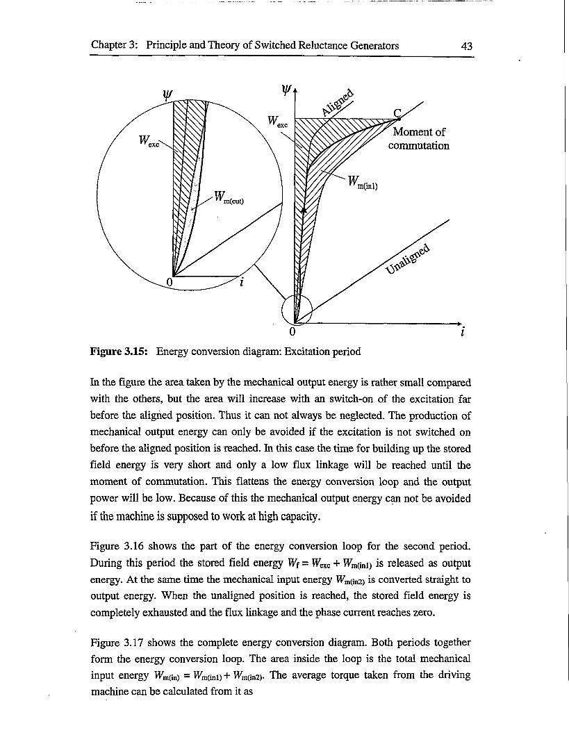
Figure 3.15 shows the part of the energy conversion diagram for the first period.
During this period the excitation energy WeXC combines with the mechanical input
energy W^mi; to build up the stored field energy Wf. No energy is supplied to the
output during this period. It is all stored in the magnetic field.
The magnified part of figure 3.15 shows the mechanical output energy Wm(0Ut). It is a
part of the energy supplied by the source but it is not stored in the magnetic field.
Instead it is converted to mechanical work and produces a small positive torque. This
is caused by the switch-on of the excitation before the aligned position is reached. It
seems that the mechanical output energy is wasted in the generating operation, but
the produced positive torque can be used by another phase depending on the number
of phases, the position in which the excitation will be switched on and the moment of
commutation. If these dependencies suit, the torque will be taken over straight from
another phase and thus the necessary driving torque will be decreased.
Chapter 3: Principle and Theory of Switched Reluctance Generators 43
Moment of commutation
m(out)
Figure 3.15: Energy conversion diagram: Excitation period
In the figure the area taken by the mechanical output energy is rather small compared
with the others, but the area will increase with an switch-on of the excitation far
before the aligned position. Thus it can not always be neglected. The production of
mechanical output energy can only be avoided if the excitation is not switched on
before the aligned position is reached. In this case the time for building up the stored
field energy is very short and only a low flux linkage will be reached until the
moment of commutation. This flattens the energy conversion loop and the output
power will be low. Because of this the mechanical output energy can not be avoided
if the machine is supposed to work at high capacity.
Figure 3.16 shows the part of the energy conversion loop for the second period.
During this period the stored field energy Wf = Wexc + Wm(ini) is released as output
energy. At the same time the mechanical input energy Wm(in2) is converted straight to
output energy. When the unaligned position is reached, the stored field energy is
completely exhausted and the flux linkage and the phase current reaches zero.
Figure 3.17 shows the complete energy conversion diagram. Both periods together
form the energy conversion loop. The area inside the loop is the total mechanical
input energy = Wm(i„i) + Wm(in2). The average torque taken from the driving
machine can be calculated from it as

Chapter 3: Principle and Theory of Switched Reluctance Generators 44
(3.26)
The mechanical input power equals the effective output energy if the excitation
current is taken from the same source than the output current is provided to.
Depending on the commutation circuit different sources for excitation and output are
possible (see chapter 3.3.3). Then the excitation energy has to be added to the total mechanical input energy to get the total input energy. Also the total output energy is
increased by the excitation energy.
0 i
Figure 3.16: Energy conversions diagram: Output period
The output capability of switched reluctance generators clearly depends on the
available area of the i-y/ diagram. To achieve a high specific output, it is important to
have a large inductance ratio and a high aligned saturation flux linkage. This ensures
a large usable area for the energy conversion loop between the unaligned and aligned
magnetisation curves.
The energy flow in a switched reluctance generator can be characterised by the
excitation penalty
(3.27)
with Pexc as the average electrical excitation power and Pout as the average electrical
output power. Ideally the excitation penalty would be zero, but this is impossible

Chapter 3: Principle and Theory of Switched Reluctance Generators 45
because it would require a zero air gap and non-saturable iron. Thus the excitation
penalty should be as small as possible.
Figure 3.17: Complete energy conversion diagram
If the excitation and output sources are equal, the efficiency is
77 = -out (3.28)
1 mech
with Pmech as the mean mechanical input power. For different sources the efficiency
is
V = P + px exc 1 mech(3.29)
3.3 Commutation Unit
Switched reluctance generators need essentially a commutation unit, because
unipolar current pulses have to be supplied every stroke for excitation. The
magnitude and amplitude of the excitation current pulses have to be controlled to
fulfil the requirements of the output power control and of the commutation
components. Also a reverse voltage has to be supplied for demagnetisation to get the
output current. The commutation in the converter is a current commutation. This
means that the current in one phase has to be reduced to zero and the current in the
following phase build up from zero.
Chapter 3: Principle and Theory of Switched Reluctance Generators 46
The commutation unit is required to raise the current in the on-going phase in the
minimum time to get enough excitation and to minimise current disturbances. For
this it needs a sufficiently high forcing voltage at each operation point, so that the current is injected quickly enough into the winding. This is critical at high speeds
since the available time is decreased, because the time for excitation is inversely
proportional to the rotation speed. At low speeds the current has to be limited
because of appearing high current peaks which could destroy the commutation
components. It also has to have a high demagnetising voltage to provide efficient
energy extraction during the demagnetisation interval, which is important for a highly
cyclical energy exchange between the converter and the generator, and it has to
permit an extension of the excitation period.
Another requirement is to provide independent control of the phase currents for the
possibility of an overlap, so that excitation can be supplied to one phase while
extracting it simultaneously from the other phase. Obvious requirements are high
efficiency, low switch to phase ratio and as low converter power rating as possible to
save production costs, high reliability and robustness and low noise and current
pulsation. The converter current rating is determined at low speeds, whereas the
voltage rating is fixed by the maximum speed.
The converter topologies can be distinguished into groups by the voltages used for
magnetisation and demagnetisation and their ability to provide independent phase
control. Single-rail circuits are characterised by having the same voltage available for
magnetisation and demagnetisation, whereas dual-rail circuits use different voltages.
Single phase circuits allow an independent control of each phase, whereas multiple
phase circuits can not cope with phase overlap. These are the key parameter that
affect the inverter selection, and most important is whether the generator operates
with or without an overlapping current through its speed range.
Lots of effort has been lately put on the task to develop new and cheap converter
topologies for motoring operation, as it can be seen from the literature
[4],[7],[13],[18], [19],[40]. The main attempt was to reduce the number of switches
per phase, and many different converter circuits with a reduced amount of switches
have been designed. Other publications concentrate on comparative evaluations like
[49] and a basic general overview is given in references [27],[48]. Every converter
circuit mentioned in the literature can not be used for generating operation because
some of them do not allow to deliver energy to the source during the demagnetisation
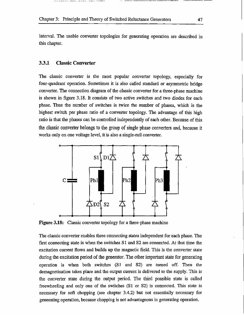
Chapter 3: Principle and Theory of Switched Reluctance Generators 47
interval. The usable converter topologies for generating operation are described in
this chapter.
3.3.1 Classic Converter
The classic converter is the most popular converter topology, especially for
four-quadrant operation. Sometimes it is also called standard or asymmetric bridge
converter. The connection diagram of the classic converter for a three-phase machine
is shown in figure 3.18. It consists of two active switches and two diodes for each
phase. Thus the number of switches is twice the number of phases, which is the
highest switch per phase ratio of a converter topology. The advantage of this high
ratio is that the phases can be controlled independently of each other. Because of this
the classic converter belongs to the group of single phase converters and, because it
works only on one voltage level, it is also a single-rail converter.
S1\D1A
Figure 3.18: Classic converter topology for a three-phase machine
The classic converter enables three connecting states independent for each phase. The
first connecting state is when the switches SI and S2 are connected. At that time the
excitation current flows and builds up the magnetic field. This is the converter state
during the excitation period of the generator. The other important state for generating
operation is when both switches (SI and S2) are turned off. Then the demagnetisation takes place and the output current is delivered to the supply. This is
the converter state during the output period. The third possible state is called
freewheeling and only one of the switches (SI or S2) is connected. This state is
necessary for soft chopping (see chapter 3.4.2) but not essentially necessary for
generating operation, because chopping is not advantageous in generating operation.

Chapter 3: Principle and Theory of Switched Reluctance Generators 48
The classic converter has many advantages. The most important is that the current
overlap does not affect. Thus the phases can be controlled independently. The full
supply voltage is applied to the winding in either direction of polarity and the
components have a low voltage rating. It has also some disadvantages of which the
most significant is the high total number of switches which equals a high switch to
phase ratio. Others are the need of a DC link filter, the low demagnetisation voltage
at high speeds and the high voltage drop across the converter switches which is a
significant fraction of the supply voltage in low-voltage applications.
3.3.2 (n+l)-switch converter
The (n+l)-switch converter is named after the number of switches used. The number
of switches is one higher than the number of phases. This is one switch more than the
minimum possible number (for example compare chapters 3.3.3 and 3.3.4). Sometimes this converter is also called Miller or common switch converter. It is
derived from the classic converter by substituting switches and diodes. The
connection diagram of the (n+l)-switch converter for a three-phase machine is shown
in figure 3.19. It consists of one common diode and active switch for all phases and
another diode and active switch for each phase. The disadvantage of the low switch
per phase ratio is that the phases can not be controlled independently of each other.
The (n+l)-switch converter belongs to the group of multiple phase and single-rail
converters.
Figure 3.19: (n+l)-switch converter for a three-phase machine
Like the classic converter, also the (n+l)-switch converter enables the three
connecting states for excitation, output and freewheeling. The main limitation is that
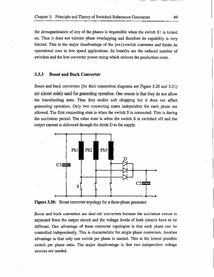
Chapter 3: Principle and Theory of Switched Reluctance Generators 49
the demagnetisation of any of the phases is impossible when the switch SI is turned
on. Thus it does not tolerate phase overlapping and therefore its capability is very
limited. This is the major disadvantage of the (n+1)-switch converter and limits its
operational area to low speed applications. Its benefits are the reduced number of
switches and the low converter power rating which reduces the production costs.
3.3.3 Boost and Buck Converter
Boost and buck converters (for their connection diagrams see Figure 3.20 and 3.21)
are almost solely used for generating operation. One reason is that they do not allow
the freewheeling state. Thus they enable soft chopping but it does not affect
generating operation. Only two connecting states independent for each phase are
allowed. The first connecting state is when the switch S is connected. This is during
the excitation period. The other state is when the switch S is switched off and the
output current is delivered through the diode D to the supply.
Figure 3.20: Boost converter topology for a three-phase generator
Boost and buck converters are dual-rail converters because the excitation circuit is
separated from the output circuit and the voltage levels of both circuits have to be
different. One advantage of these converter topologies is that each phase can be
controlled independently. This is characteristic for single phase converters. Another
advantage is that only one switch per phase is needed. This is the lowest possible
switch per phase ratio. The major disadvantage is that two independent voltage
sources are needed.

Chapter 3: Principle and Theory of Switched Reluctance Generators 50
Characteristic for boost converters is that the output voltage has to exceed the input
voltage. This leads to a problem at slow speeds because the high reverse voltage
across the phase winding extinguishes the flux too quickly and the energy conversion
is cut off with only a fraction of its maximum possible output. The boost converter is
sometimes also called up converter
Figure 3.21: Buck converter topology for a three-phase generator
Buck converters are characterised by a lower output voltage than input voltage. This
has the advantage that the problem of boost converters does not appear in buck
converters. The lower output voltage leads to a longer output period with a slower
extinction of the flux. A higher output can be reached because a fuller energy
conversion loop is obtained. The buck converter is sometimes also called down
converter.
3.3.4 Bifilar Winding Converter
The bifilar winding converter, like the boost and buck converters, uses the smallest
possible number of power devices. Just one switch is required per phase and this
leads to the lowest possible switch per phase ratio. Figure 3.22 shows the connection
diagram of a bifilar winding converter for a three-phase machine. The converter
allows two connecting states independent for each phase. At first, when the switch S
is connected, the magnetic field for the excitation is build up. After the switch S is
switched off, the output current is delivered through the diode D to the supply. These
are the two possible states. The bifilar winding converter can not operate in the
freewheeling state and thus soft chopping is enabled, which does not affect generating operation.
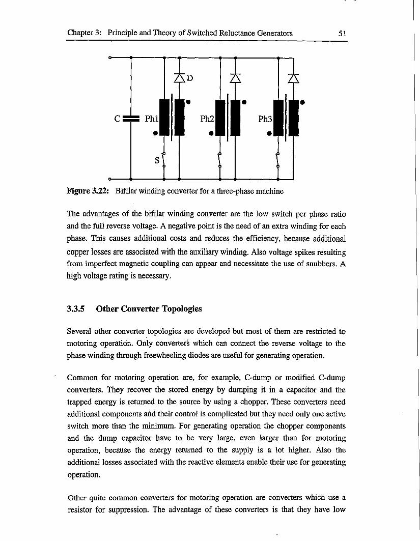
Chapter 3: Principle and Theory of Switched Reluctance Generators 51
O-
Ad A A
s
O'Figure 3.22: Bifilar winding converter for a three-phase machine
The advantages of the bifilar winding converter are the low switch per phase ratio
and the full reverse voltage. A negative point is the need of an extra winding for each
phase. This causes additional costs and reduces the efficiency, because additional
copper losses are associated with the auxiliary winding. Also voltage spikes resulting from imperfect magnetic coupling can appear and necessitate the use of snubbers. A
high voltage rating is necessary.
3.3.5 Other Converter Topologies
Several other converter topologies are developed but most of them are restricted to
motoring operation. Only converters which can connect the reverse voltage to the
phase winding through freewheeling diodes are useful for generating operation.
Common for motoring operation are, for example, C-dump or modified C-dump
converters. They recover the stored energy by dumping it in a capacitor and the
trapped energy is returned to the source by using a chopper. These converters need
additional components and their control is complicated but they need only one active
switch more than the minimum. For generating operation the chopper components
and the dump capacitor have to be very large, even larger than for motoring
operation, because the energy returned to the supply is a lot higher. Also the
additional losses associated with the reactive elements enable their use for generating
operation.
Other quite common converters for motoring operation are converters which use a
resistor for suppression. The advantage of these converters is that they have low
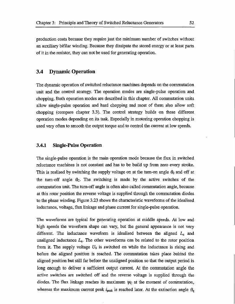
Chapter 3: Principle and Theory of Switched Reluctance Generators 52
production costs because they require just the minimum number of switches without
an auxiliary bifilar winding. Because they dissipate the stored energy or at least parts
of it in the resistor, they can not be used for generating operation.
3.4 Dynamic Operation
The dynamic operation of switched reluctance machines depends on the commutation
unit and the control strategy. The operation modes are single-pulse operation and
chopping. Both operation modes are described in this chapter. All commutation units
allow single-pulse operation and hard chopping and most of them also allow soft
chopping (compare chapter 3.3). The control strategy builds on these different
operation modes depending on its task. Especially in motoring operation chopping is
used very often to smooth the output torque and to control the current at low speeds.
3.4.1 Single-Pulse Operation
The single-pulse operation is the main operation mode because the flux in switched
reluctance machines is not constant and has to be build up from zero every stroke.
This is realised by switching the supply voltage on at the turn-on angle 6q and off at
the turn-off angle 6c- The switching is made by the active switches of the
commutation unit. The turn-off angle is often also called commutation angle, because
at this rotor position the reverse voltage is supplied through the commutation diodes
to the phase winding. Figure 3.23 shows the characteristic waveforms of the idealised
inductance, voltage, flux linkage and phase current for single-pulse operation.
The waveforms are typical for generating operation at middle speeds. At low and
high speeds the waveform shape can vary, but the general appearance is not very
different. The inductance waveform is idealised between the aligned La and
unaligned inductance L^. The other waveforms can be related to the rotor position
from it. The supply voltage Us is switched on while the inductance is rising and
before the aligned position is reached. The commutation takes place behind the
aligned position but still far before the unaligned position so that the output period is
long enough to deliver a sufficient output current. At the commutation angle the active switches are switched off and the reverse voltage is supplied through the
diodes. The flux linkage reaches its maximum y/c at the moment of commutation,
whereas the maximum current peak /peak is reached later. At the extinction angle 9q

Chapter 3: Principle and Theory of Switched Reluctance Generators 53
the voltage, flux linkage and phase current are back to zero and the diodes are closed
again.
Idealised inductance
Aligned
Unaligned
Voltage
Flux linkage
■ Phase current
Excitationperiod
Figure 3.23: Single-pulse waveforms for generating operation
Ideally the switch-on angle should be close to the aligned position because otherwise
a small positive torque is produced by the supply current of the battery. On the other
hand, the excitation will not be sufficient if the period is too short. Especially at high
speeds the disadvantage of positive torque production has to be accepted (compare
chapter 3.2.4). The angle difference between the turn-off and the tum-on angle is
called dwell angle It is the angle that stretches across the excitation period. The
control of switched reluctance machines uses both the tum-on and the turn-off and
thus also the dwell angle. In generating operation the output power and the height of
the peak currents are depending on these angles.

Chapter 3: Principle and Theory of Switched Reluctance Generators 54
3.4.2 Chopping
Chopping is necessary in motoring operation to control the current at low speeds and
to smooth the output torque. It is realised by using the freewheeling or reversing state
of the commutation unit which were already explained in chapter 3.3. The types ofchopping are distinguished in voltage pulse-width modulation and current regulation.
Both types of chopping can be realised by soft and hard chopping. In soft chopping
the supply voltage is switched off by using the freewheeling state, whereas in hard
chopping the voltage is reversed by using the reversing state of the commutation unit.
The characteristic of voltage pulse-width modulation is that the state of the
commutation unit is switched at high frequency with a fixed duty cycle during the
dwell period. For current regulation the state is switched during the dwell period
depending on the current being greater or smaller than a reference current. Thus the
duty cycle is variable.
Chopping is not advantageous in generating operation because the peak of the output
current appears during the output period and not during the excitation or dwell period
(see chapter 3.4.1) when chopping is used. Thus chopping reduces only the excitation
current but that is not desirable and has no direct influence on the peak of the output
current. Other strategies have to be used to reduce the high peak of the output
current, especially at slow speeds.
3.5 Control System
Switched reluctance machines need a control system because the current waveform
shape and its magnitude must be controlled in relation to the variations of speed and
load. This task is quite difficult to fulfil because the relationships between torque,
current, speed and firing angles are highly non-linear and vary as a function of speed
and load. The control strategy has to cope with these difficulties and sometimes it has
to fulfil also the requirements of peak current regulation. Another difficulty is that
switched reluctance machines have no axis transformation like AC motors and no
field oriented control principle has been developed for them. Thus it is necessary to
use high-speed real time controllers which operate with phase currents and voltages
directly. Also the switching precision is critical in switched reluctance drives and a
precision of 0.5° or even 0.25° is desirable, as it is pointed out in reference [27].
Motors are normally controlled by closed-loop speed and sometimes torque control,
whereas generators are controlled by keeping the output voltage constant. The

Chapter 3: Principle and Theory of Switched Reluctance Generators 55
parameters for the control are the turn-on and the turn-off angles. A rotor position
feedback is necessary to synchronise the switching of the commutation devices
depending on the firing angles with the rotor position. The rotor position can be
obtained by direct or indirect sensing. The conventional way is to use direct position
sensing and it is realised by using a slotted disk together with optical interrupters,
Hall-effect or other type of sensors. The indirect rotor position sensing is a popular
field for investigations and research and many articles have been published, like
[8],[9],[16],[21],[23],[36],[37],[38]. It is described later in this chapter.
3.5.1 Structure
The structure of the control system for switched reluctance generators is shown in
figure 3.24. The controller, commutation unit and switched reluctance generator are
considered as a black box for the reason of simplicity. The system input value is a
reference voltage UKfwhich is generally kept constant depending on the voltage level
of the source and loads. The system output is the output voltage Uout of the generator
and varies with load and speed. It has to be kept constant and thus a voltage error AU is derived by comparison with the reference voltage after feedback. The voltage error
together with the rotor position 6 and angular velocity (0 feedback is the input of the
controller which has to estimate the firing angles 0O and 0c for the commutation unit.
The commutation unit then switches the phase currents i\, i% and h of the generator.
This all put together results in the structure of the control system.
AU CommutationUnit
Controller SR-Generator
Figure 3.24: Control system structure for a three-phase generator
3.5.2 Control Modes and Strategy
Different control modes for switched reluctance motors are mentioned in the
literature [3],[27]. The modes are normal, boost and long dwell and are distinguished
according to the values of the firing angles and the resulting characteristics. The
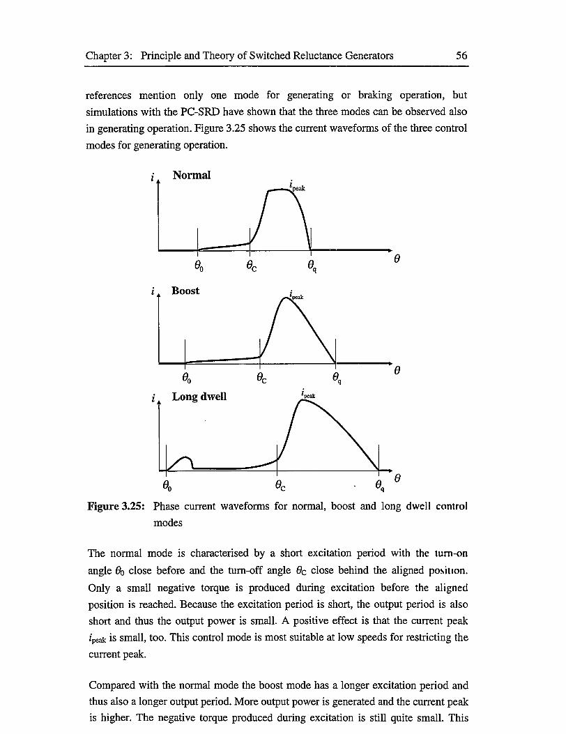
Chapter 3: Principle and Theory of Switched Reluctance Generators 56
references mention only one mode for generating or braking operation, but
simulations with the PC-SRD have shown that the three modes can be observed also
in generating operation. Figure 3.25 shows the current waveforms of the three control
modes for generating operation.
Normal
Boost
Long dwell
Figure 3.25: Phase current waveforms for normal, boost and long dwell control
modes
The normal mode is characterised by a short excitation period with the tum-on
angle 6q close before and the turn-off angle 0c close behind the aligned position.
Only a small negative torque is produced during excitation before the aligned
position is reached. Because the excitation period is short, the output period is also
short and thus the output power is small. A positive effect is that the current peak
/peak is small, too. This control mode is most suitable at low speeds for restricting the
current peak.
Compared with the normal mode the boost mode has a longer excitation period and
thus also a longer output period. More output power is generated and the current peak
is higher. The negative torque produced during excitation is still quite small. This
Chapter 3: Principle and Theory of Switched Reluctance Generators 57
mode should be used at medium speeds. Because of the higher speed a longer
excitation period is needed to reach the nominal output power.
The long dwell or also called the advanced mode has the longest excitation period
with the turn-on angle far before and turn-off angle far after the aligned position. The
first smaller current peak of the current waveform for the long dwell mode, which
can be seen in the figure, produces a worth mentioning negative torque because of the
turn-on of the excitation far before the aligned position. The output period isextended and thus a high output power is reached. A negative feature is the high
output current peak. This mode is supposed to be used at high and very high speeds
to reach a high output power. There is no clear distinction between the modes.
Basically the control strategy can be realised in two ways. The first and the easier
possibility is to vary just the turn-on angle and to keep the turn-off angle constant at a
sufficiently high value. This has the consequence that very high current peaks can
appear at low speeds together with high load, which may not be tolerated by the
commutation unit. At low load the ratio of peak current and RMS-current can be
high, but these current peaks will not cause damage to the commutation, because
their level is lower than in the other situation. This control strategy is mainly based
on the long dwell mode with the turn-off angle far behind the aligned position.
The other possibility is to vary both firing angles. Then a smoother output current
waveform is reached and the critical high current peaks are avoided. The reason for
this is that all control modes are used in their suitable speed ranges. This control
strategy is more sophisticated but has the mentioned major advantages.
3.5.3 Sensorless Control
The sensorless control can be distinguished into four schemes. The schemes are
open-loop control, passive waveform detection, active probing and observers. In
open-loop control the dwell period is controlled but the firing angles are not
synchronised to the rotor position. These controllers are unstable and they have to be
stabilised by using other external values, like torque or current, to recognise load or
speed changes. They are not useful in generating operation because the firing angles
have to be kept exactly in position to keep the output voltage constant and to avoid
high current peaks.

Chapter 3: Principle and Theory of Switched Reluctance Generators 58
The passive waveform detection mainly relies on characteristics in the phase current
waveform, for example maximum or minimum. Phase current measurements are
necessary to realise this scheme. Reference [23] illustrates the realisation of such a
scheme that detects the change of current ripple and converts it to a rotor position
signal, but it can provide the signal only at low speeds. References [36],[37],[38]
describe a sensing technique that uses the current rise and fall times. Restrictions to
low speeds are mentioned and the successful detection of the rotor position is related to chopping operation. Another method is to measure the mutual induced voltage in
an unexcited phase as it is described in reference [16]. It is suitable for low speeds,
low voltage and high current drives with single switch per phase converters. In
generating operation passive waveform detection does not seem very suitable
because the high current peaks appear at low speeds and thus switched reluctance
generators should operate at higher speeds.
For sensing with active probing, a square-wave voltage is applied to an unexcited
phase. The resulting current pulses vary with the phase inductance. The minimum
and the maximum are reached with the aligned and unaligned positions. The rotor
position can be detected from this. The references [8],[9],[21] describe the realisation
of position sensing with active probing. Problems occur with a small number of
phases because of phase overlap and the references mention that the realisation is
most reliable for machines with at least three or preferably four phases.
The most demanding control scheme uses observers. A state observer is a mathematical simulation of the machine running on-line on a microcomputer in
parallel with the drive. Measured currents and voltages are the input for a model
which gives then the rotor position and speed.

59
4 Generator Design
Before the generator design can be made, some suppositions have to be defined. The
main suppositions are supply voltage, speed-range and size. A common 12 V battery
is chosen for the power supply, as it is used in motor vehicles. This is the cheapest
and most reliable solution. It also opens the easiest possibility of using the generator
in the most common field of applications - in motor vehicles. A detailed description
of battery characteristics is given in the references [14] and [17].
Table 4.1 includes the main battery characteristics. It can be seen that different
characteristic voltages are necessary to describe the battery behaviour because the
voltage depends on the state of charge. Besides the conventional nominal voltage
also rest, discharged, maximum charged and gassing voltages are introduced. Also
the nominal capacity is included. This capacity is defined by the amount of current
which can be delivered during 20 hours of discharging at 27° C with a constant
current.
Table 4.1: Main battery characteristics
Nominal voltage C/N= 12 VRest voltage U rest = 12.72 VDischarged voltage t/dis= 11.76... 11.88 VMaximum charged voltage Umax = 15.6 ... 16.2 VGassing voltage UR as = 14.4 VNominal capacity K 20 = 84 Ah
The voltage drops down to the rest voltage after charging of the battery and it will be
held. If the battery is partly discharged, the rest voltage will be reached after a few
seconds of charging. The lowest possible voltage is reached when the battery is
discharged. Analogously the maximum voltage is reached when the battery is fully
charged but before reaching that level the battery water will start to decompose at the gassing voltage. Thus the gassing voltage should not be exceeded. Figure 4.1
illustrates this voltage behaviour versus time for charging and discharging.
The voltage behaviour of batteries is also depending on the temperature. The above
mentioned values of the voltage levels are applied to 20° C and they decrease in
colder surroundings. Thus a voltage of 14 V has been chosen as operating voltage of
the generator to surely avoid the decomposition of the battery water at the gassing
voltage of 14.4 V. It also provides some clearance for the control system.

Chapter 4: Generator Design 60
UN14.4 t
13.8 "
13.2 --
— Charging —Discharging
12.0 --
11.4 --
0123456789 10
Figure 4.1: Battery voltage versus time for charging and discharging
The speed range of the generator is chosen according to the speed range of the
internal combustion engine of motor vehicles to provide the best output characteristic
for this main application. A speed range multiplied by a constant ratio factor is also
suitable. This can be realised by the variation of the pulley size. It can be suited in the
same way for other applications with a different speed range. The speed range of
combustion engines spans from the idling speed 800 rpm up to 8,000 rpm. At a speed
of 6,000 rpm the overspeed range begins, so this range is rarely used for driving.
Speeds around 3,000 to 4,000 rpm are used mostly.
The size of the switched reluctance generator should be around the size of large
alternators for 12 V applications. Then the new generator with its supposed higher
output power would be advantageous in this point. The outer stator diameter of these
alternators is around 150 mm, the outer length is usually a bit smaller than the
diameter and the weight is around 7 kg.
4.1 Construction
Before geometrical details of the construction can be designed the magnetic material
has to be chosen because it has a major influence on the machine performance. Its
typical magnetic values, magnetisation curve, core losses and mechanical properties
have to be known before a design can be made. The material has to fulfil the special
demands of switched reluctance machines, like high commutation frequency, high
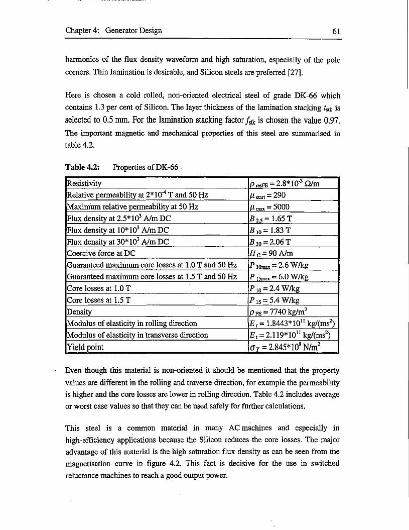
Chapter 4: Generator Design 61
harmonics of the flux density waveform and high saturation, especially of the pole
comers. Thin lamination is desirable, and Silicon steels are preferred [27].
Here is chosen a cold rolled, non-oriented electrical steel of grade DK-66 which
contains 1.3 per cent of Silicon. The layer thickness of the lamination stacking rstk is
selected to 0.5 mm. For the lamination stacking factor fs± is chosen the value 0.97.
The important magnetic and mechanical properties of this steel are summarised in
table 4.2.
Table 4.2: Properties of DK-66
Resistivity P resFE = 2.8* 10'3 £2/mRelative permeability at 2*104 T and 50 Hz P start — 290
Maximum relative permeability at 50 Hz P max = 5000Flux density at 2.5* 103 A/m DC B 25= 1.65 TFlux density at 10* 103 A/m DC B io= 1.83 TFlux density at 30* 103 A/m DC B 30 = 2.06 TCoercive force at DC Hc = 90 A/mGuaranteed maximum core losses at 1.0 T and 50 Hz P 10max = 2.6 w/kgGuaranteed maximum core losses at 1.5 T and 50 Hz P 15max = 6.0 w/kgCore losses at 1.0 T f 10 = 2.4 W/kgCore losses at 1.5 T P15 = 5.4 W/kgDensity Pfe = 7740 kg/m3Modulus of elasticity in rolling direction £r=1.8443*10nkg/(ms2)
Modulus of elasticity in transverse direction £, = 2.119*10n kg/(ms2)
Yield point C7y=2.845*108N/m2
Even though this material is non-oriented it should be mentioned that the property
values are different in the rolling and traverse direction, for example the permeability
is higher and the core losses are lower in rolling direction. Table 4.2 includes average
or worst case values so that they can be used safely for further calculations.
This steel is a common material in many AC machines and especially in
high-efficiency applications because the Silicon reduces the core losses. The major
advantage of this material is the high saturation flux density as can be seen from the
magnetisation curve in figure 4.2. This fact is decisive for the use in switched
reluctance machines to reach a good output power.

Chapter 4: Generator Design 62
2.00 •
1.80 ■
1.00-
0.40 •
0.20*
2.00 2.60 3.000.60Ax* x 1.0*4
Figure 4.2: Magnetisation curve of DK-66 as integrated into the PC-SRD
4.1.1 Basic Characteristics
In order to get a competitive machine the number of phases should be as low as
possible. This guarantees low production costs because of the easy construction and a
commutation unit with a small amount of switches. A one-phase generator has the
minimum number of phases but it has only an absolute current output zone of one
half. This means that output current can be produced maximum over only one half of
each revolution. The other half of the revolution is over a blank zone and can not be
used for current generation. This is definitely too low utilisation of a machine. To get
output current almost over a full revolution the absolute current zone has to be at
least one. This together with the already mentioned demand fulfils a two-phase
generator. Thus a two-phase generator is chosen.
Table 3.1 shows two different possible rotor and stator pole combinations for
two-phase machines. In reference [20] the influence of the number of poles per phase
in switched reluctance motors has been researched. It concludes that both single- and
multiple-pole-pair-per-phase motors have their advantages depending on the
application. Because of this an analysis of two-phase generators with single- and
multiple-pole-pairs-per-phase has been made with the PC-SRD in this work to
examine the influence for generator applications. The results show that the generator
with eight stator poles and four rotor poles has only disadvantages compared with the
other one. The peak currents are higher, a more precise controller is needed and the
geometry is more complicated. Thus the number of stator poles is chosen to 4 and the

Chapter 4: Generator Design 63
number of rotor poles to 2 respectively. Then the stroke angle is 90° and the number
of strokes per revolution is 4.
4.1.2 Envelope and Internal Dimensions
For the design of the geometrical dimensions a starting point has to be found to
enable simulations with the PC-SRD. This can be done by solving equation (3.1) for
typical values. An average torque of around 10 Nm is necessary to reach the output
power of 1.5 kW at slow speeds. From table 3.2 the value for the torque per unit rotor volume can be chosen to 35 kNm/m3 to get a good performing and utilised machine.
Equation (3.1) can be solved by using these values together with a common stack
length per rotor diameter ratio of 1. Then the stack length and rotor diameter are
calculated to around 72 mm. For a rotor diameter per stator lamination diameter ratio
of 0.5 which is typical for machines with a small number of poles, the stator
lamination diameter is 144 mm. This fulfils the supposition for the approximated
generator size and with a stack length of 72 mm the overall length will be also less
than 150 mm.
A large shaft diameter is desirable to maximise the lateral stiffness of the rotor. It
raises the first critical resonance speed and reduces the acoustic noise. Thus the shaft
diameter is chosen quite large to 20 mm. The rotor yoke has to be sufficient to carry
the rotor flux, which means, that it should be at least half the rotor pole width,
because the flux divides into two equal parts when it leaves the rotor poles. For a
rotor yoke of half the rotor pole width the minor rotor diameter can be calculated by
Am = Ah+ tT with tT given by equation (3.2). For a typical rotor pole arc of 45° the
result is 47.5 mm (for the pole arc selection and optimisation see chapter 4.1.3).
The air gap length is initially chosen to 0.5 mm. This is larger than the minimum
limit of 0.2 mm which is caused by the very difficult production situation under this
limit. The last missing parameter value is the stator slot bottom diameter. The facts for the stator yoke are equal to those for the rotor yoke except that the stator yoke
thickness has in addition a major influence on the acoustic noise of the generator.
Thus the stator yoke should be chosen thicker than ts /2 to increase the stiffness and thus to reduce acoustic noise. A suitable value is 2/3 ts. The stator slot bottom
diameter can be calculated by Dsb = DS- 4/3 ts with ts given by equation (3.3). With a
typical stator pole arc of 45° it equals to 106.5 mm.
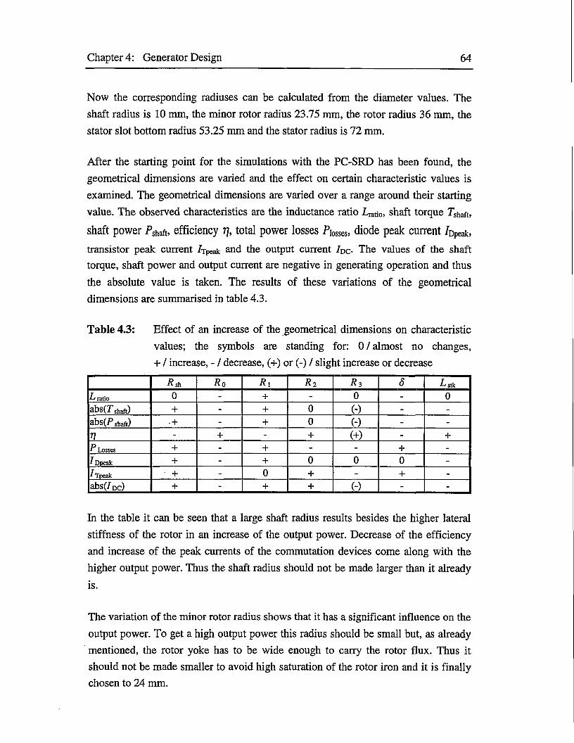
Chapter 4: Generator Design 64
Now the corresponding radiuses can be calculated from the diameter values. The
shaft radius is 10 mm, the minor rotor radius 23.75 mm, the rotor radius 36 mm, the
stator slot bottom radius 53.25 mm and the stator radius is 72 mm.
After the starting point for the simulations with the PC-SRD has been found, the
geometrical dimensions are varied and the effect on certain characteristic values is
examined. The geometrical dimensions are varied over a range around their starting
value. The observed characteristics are the inductance ratio L^o, shaft torque Tshaft,
shaft power fshaft, efficiency t}, total power losses P\0sses, diode peak current /Dpeak,
transistor peak current /rpeak and the output current /Dc. The values of the shaft torque, shaft power and output current are negative in generating operation and thus
the absolute value is taken. The results of these variations of the geometrical dimensions are summarised in table 4.3.
Table 4.3: Effect of an increase of the geometrical dimensions on characteristic
values; the symbols are standing for: 0 / almost no changes,
+ / increase, - / decrease, (+) or (-) / slight increase or decrease
R sh Ro Ri Ri R 3 8 •t-stk
1* ratio 0 - + - 0 - 0
abs(7 shaft) + - + 0 (-) - -
abs(P shaft) ■ + - + 0 (-) - -
77 - + - + (+) - +
P Losses + - + - - + -
I Dpeak + - + 0 0 0 -
f Tpeak ■ + - 0 + - + -
abs(/Dc) + - + + (-) - -
In the table it can be seen that a large shaft radius results besides the higher lateral
stiffness of the rotor in an increase of the output power. Decrease of the efficiency
and increase of the peak currents of the commutation devices come along with the
higher output power. Thus the shaft radius should not be made larger than it already
is.
The variation of the minor rotor radius shows that it has a significant influence on the
output power. To get a high output power this radius should be small but, as already
mentioned, the rotor yoke has to be wide enough to carry the rotor flux. Thus it
should not be made smaller to avoid high saturation of the rotor iron and it is finally
chosen to 24 mm.
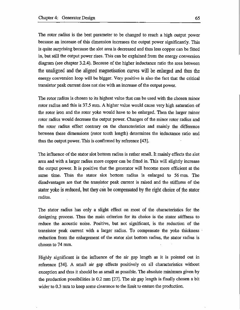
Chapter 4: Generator Design 65
The rotor radius is the best parameter to be changed to reach a high output power
because an increase of this dimension increases the output power significantly. This
is quite surprising because the slot area is decreased and thus less copper can be fitted
in, but still the output power rises. This can be explained from the energy conversion
diagram (see chapter 3.2.4). Because of the higher inductance ratio the area between
the unaligned and the aligned magnetisation curves will be enlarged and thus the
energy conversion loop will be bigger. Very positive is also the fact that the critical
transistor peak current does not rise with an increase of the output power.
The rotor radius is chosen to its highest value that can be used with the chosen minor
rotor radius and this is 37.5 mm. A higher value would cause very high saturation of
the rotor iron and the rotor yoke would have to be enlarged. Then the larger minor
rotor radius would decrease the output power. Changes of the minor rotor radius and
the rotor radius effect contrary on the characteristics and mainly the difference
between these dimensions (rotor tooth length) determines the inductance ratio and
thus the output power. This is confirmed by reference [43].
The influence of the stator slot bottom radius is rather small. It mainly effects the slot
area and with a larger radius more copper can be fitted in. This will slightly increase
the output power. It is positive that the generator will become more efficient at the
same time. Thus the stator slot bottom radius is enlarged to 56 mm. The
disadvantages are that the transistor peak current is raised and the stiffness of the
stator yoke is reduced, but they can be compensated by the right choice of the stator
radius.
The stator radius has only a slight effect on most of the characteristics for the
designing process. Thus the main criterion for its choice is the stator stiffness to
reduce the acoustic noise. Positive, but not significant, is the reduction of the
transistor peak current with a larger radius. To compensate the yoke thickness
reduction from the enlargement of the stator slot bottom radius, the stator radius is
chosen to 74 mm.
Highly significant is the influence of the air gap length as it is pointed out in
reference [34]. A small air gap effects positively on all characteristics without
exception and thus it should be as small as possible. The absolute minimum given by
the production possibilities is 0.2 mm [27]. The air gap length is finally chosen a bit
wider to 0.3 mm to keep some clearance to the limit to ensure the production.

Chapter 4: Generator Design 66
An increase of the stack length gives lower peak currents and the efficiency will be
higher, but on the other hand the output power will be decreased. Thus a good
compromise between these characteristics has to be found. Because the influence on the peak currents is more sufficient the stack length is chosen to 75 mm. A small
stack length also enlarges the influence of end effects. The effect of end core flux on
the machine performance is presented in reference [24].
The optimum choice of the values of all dimensions had been verified for different
speeds and load conditions. From these finally settled dimensions the longitudinal generator cross section can be drawn. It is shown scaled down in figure 4.3 and truly
scaled in figure B.2 in Appendix B.
Figure 4.3: Longitudinal cross section of the generator
4.1.3 Pole Size and Geometry
The stator and the rotor poles have to be designed. The pole sizes are determined
mainly by the stator and rotor pole arcs. The other dimensions effecting on the pole
sizes are already fixed in the previous chapter. A good starting point for the rotor and
stator pole arc is 45°. This value equals to half of the stroke angle and is the most
common choice because it enables output current to be produced almost during a
whole revolution and enough clearance between the rotor and stator poles.
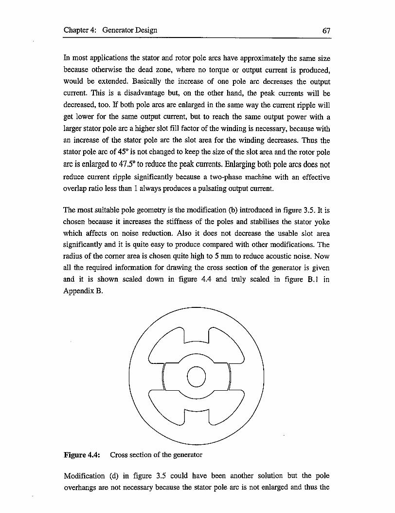
Chapter 4: Generator Design 67
In most applications the stator and rotor pole arcs have approximately the same size
because otherwise the dead zone, where no torque or output current is produced,
would be extended. Basically the increase of one pole arc decreases the output
current. This is a disadvantage but, on the other hand, the peak currents will be
decreased, too. If both pole arcs are enlarged in the same way the current ripple will
get lower for the same output current, but to reach the same output power with a
larger stator pole arc a higher slot fill factor of the winding is necessary, because with
an increase of the stator pole arc the slot area for the winding decreases. Thus the
stator pole arc of 45° is not changed to keep the size of the slot area and the rotor pole
arc is enlarged to 47.5° to reduce the peak currents. Enlarging both pole arcs does not
reduce current ripple significantly because a two-phase machine with an effective
overlap ratio less than 1 always produces a pulsating output current.
The most suitable pole geometry is the modification (b) introduced in figure 3.5. It is
chosen because it increases the stiffness of the poles and stabilises the stator yoke
which affects on noise reduction. Also it does not decrease the usable slot area
significantly and it is quite easy to produce compared with other modifications. The
radius of the comer area is chosen quite high to 5 mm to reduce acoustic noise. Now
all the required information for drawing the cross section of the generator is given
and it is shown scaled down in figure 4.4 and truly scaled in figure B.l in
Appendix B.
Figure 4.4: Cross section of the generator
Modification (d) in figure 3.5 could have been another solution but the pole
overhangs are not necessary because the stator pole arc is not enlarged and thus the
Chapter 4: Generator Design 68
slot area is large enough to fit in the winding. Different pole profiles for motoring
operation are discussed in the reference [34]. For generating operation it can not be
said if some of this profiles would be advantageous and a more complicated profile
would increase the production costs. Thus the traditional profile used with the pole
geometry in figure 3.5 is not changed.
4.1.4 Winding
The winding has a major influence on the machine performance. It determines mainly
the phase current behaviour, especially the peak current and the output power. Because of that the winding design has to be carefully and well suited.
First, the slot fill factor has to be chosen. Because of its influence on the electrical behaviour it should be as high as possible because with an increase of the slot fill
factor the output power and efficiency will be increased. Another advantage is that
the copper losses will be decreased, but the slot fill factor is limited by the geometry
of the slot and the essential insulation. The only disadvantage of a high slot fill factor
is that pre-wound windings can not be used.
Afterwards the number of turns per pole has to be chosen. Generally with an increase
in the number of turns per pole the output power and the peak current will be
decreased. A good compromise according to these two criteria has to be found and
especially at low speeds the peak currents have to be limited. Otherwise suitable
commutation devices can not be found.
The windings of opposite poles can be connected in series or parallel. Simulations
with the PC-SRD have shown that the basic machine performance does not differ
between serial and parallel connected windings if the number of turns per pole is
chosen respectively. For parallel connected windings the number of turns per pole
would have to be double compared to serial ones. Generally, serial connected
windings have a better behaviour according to the influence of harmonics. Thus
serial windings have been chosen here. The number of parallel paths per phase is
then 1.
Various simulations with the PC-SRD have shown that the optimum fixed number of
turns per pole for the serial connected winding over the whole speed range is 12. This
value provides the desired output power of 1.5 kW over a broad speed range and it
limits the peak currents at low speeds so that a good but not the desired output power

Chapter 4: Generator Design 69
can be reached at these speeds, too. Limitations of the output power at low and very
high speeds have to be made anyway if a fixed number of turns per pole is used, and
the number of turns per poles has to be fixed to realise an easy and cheap winding.
With Np that equals to 12 and %u around 0.6 the wire diameters will be very high and
with the phase current waveform high eddy current losses will be caused. A solution
for this is to use smaller wire diameters and to connect them in parallel. This has also
the advantage that a higher slot fill factor can be reached because smaller wires can
be better fitted into the given slot area geometiy. A suitable wire diameter is 1 mm.
For the above estimated generator geometry the slot area can be calculated with equation (3.6) and it is 805 mm2. The usable slot area will be decreased by the area of
the pole comers that is taken away by the radius r because of the chosen pole geometry (see chapter 4.1.3). ACOmer equals to 9.56 mm2 and is calculated from
equation (3.9) with the geometric dimensions mentioned in the previous chapters, thus the real slot area is 786 mm2. The windings have to be insulated from the stator
core iron and the two windings in the slot from each other. This will reduce the
usable slot area, too. The area taken away by an insulation layer of the thickness d around the slot and of the thickness 2d between the windings is
= 2 d (2^-2/?,-3d-25-r)+[(/?, +S+df-(R1 +S)2]^l
+ -(#2- J)2j^'°'back T ^corner _ (r~df](4.1)
withA>iot -4r(27r~NsPs)’
'slotback M\7Z-N, arcsin 5, 12
and /Corner already given by equation (3.10). The net stator slot area can then be
calculated as
Alotsnet Alois 2Acomer Ansul • (4.2)
For sufficient insulation the insulation layer thickness should be at least 0.2 mm and the net slot area then equals to 755.5 mm2.
A very suitable and common wire for all small electrical machine windings and for
many other applications is the enamelled round copper wire with DFV quality and
grade 2 insulation thickness. The wire insulation is a THEIC-modified polyester
imide enamel according to EEC 317-8 standard which has good chemical and
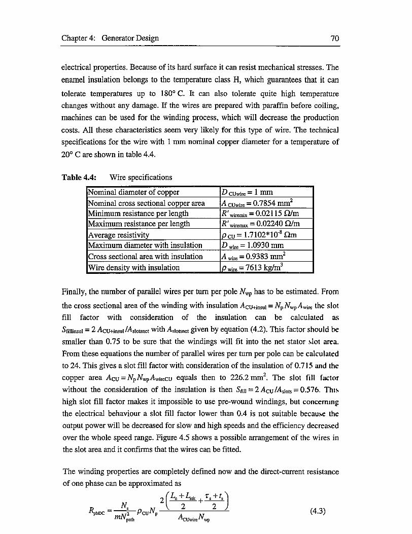
Chapter 4: Generator Design 70
electrical properties. Because of its hard surface it can resist mechanical stresses. The
enamel insulation belongs to the temperature class H, which guarantees that it can
tolerate temperatures up to 180° C. It can also tolerate quite high temperature
changes without any damage. If the wires are prepared with paraffin before coiling,
machines can be used for the winding process, which will decrease the production
costs. All these characteristics seem very likely for this type of wire. The technical
specifications for the wire with 1 mm nominal copper diameter for a temperature of
20° C are shown in table 4.4.
Table 4.4: Wire specifications
Nominal diameter of copper D CUwire — 1 Him
Nominal cross sectional copper area A cuwire = 0.7854 mm2
Minimum resistance per length R' wiremin = 0.02115 D/mMaximum resistance per length R' wiremax = 0.02240 D/m
Average resistivity Pcu= 1.7102*10-8 Dm
Maximum diameter with insulation D wire = 1.0930 mm
Cross sectional area with insulation A wire = 0.9383 mm2
Wire density with insulation P wire = 7613 kg/m3
Finally, the number of parallel wires per turn per pole jVwp has to be estimated. From
the cross sectional area of the winding with insulation Acu+insui = NpNwpAwm the slot
fill factor with consideration of the insulation can be calculated as
SfiUinsui = 2 Acu+insui/Asiotsnet with Asi0tsnet given by equation (4.2). This factor should be
smaller than 0.75 to be sure that the windings will fit into the net stator slot area.
From these equations the number of parallel wires per turn per pole can be calculated
to 24. This gives a slot fill factor with consideration of the insulation of 0.715 and the copper area Acu = 7/pMvpAwirecu equals then to 226.2 mm2. The slot fill factor
without the consideration of the insulation is then Sfm = 2 Acu/Asiots = 0.576. This
high slot fill factor makes it impossible to use pre-wound windings, but concerning
the electrical behaviour a slot fill factor lower than 0.4 is not suitable because the
output power will be decreased for slow and high speeds and the efficiency decreased
over the whole speed range. Figure 4.5 shows a possible arrangement of the wires in
the slot area and it confirms that the wires can be fitted.
The winding properties are completely defined now and the direct-current resistance
of one phase can be approximated as
(4.3)
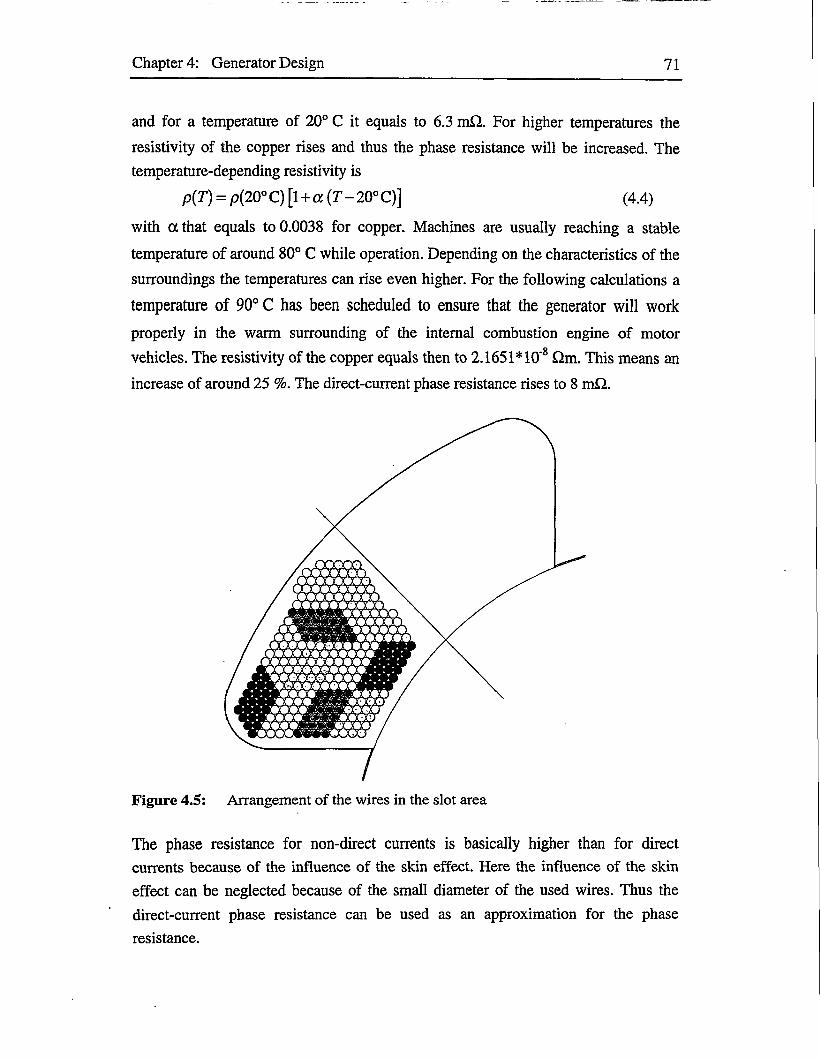
Chapter 4: Generator Design 71
and for a temperature of 20° C it equals to 6.3 m£l For higher temperatures the
resistivity of the copper rises and thus the phase resistance will be increased. The
temperature-depending resistivity is
p(T) = p(20° C) [1 + a (7-20° C)] (4.4)
with a that equals to 0.0038 for copper. Machines are usually reaching a stable
temperature of around 80° C while operation. Depending on the characteristics of the
surroundings the temperatures can rise even higher. For the following calculations a
temperature of 90° C has been scheduled to ensure that the generator will work
properly in the warm surrounding of the internal combustion engine of motor vehicles. The resistivity of the copper equals then to 2.1651*10'8 Qm. This means an
increase of around 25 %. The direct-current phase resistance rises to 8 mfl.
The phase resistance for non-direct currents is basically higher than for direct currents because of the influence of the skin effect. Here the influence of the skin
effect can be neglected because of the small diameter of the used wires. Thus the
direct-current phase resistance can be used as an approximation for the phase
resistance.
Chapter 4: Generator Design 72
4.1.5 Further Estimations
After all the basic geometrical dimensions have been set, some other interesting
values can be estimated, like the length, weight and moment of inertia. The overall
length Le can be approximated to 133.5 mm from Le = Lstk+2L0h with L„h almost equal to the stator pole width ts. For the total length of the generator the width of the
shields with the bearings and the fan must be added to the overall length, but all this
together still fulfils the previously made suppositions for the generator size.
The weight of the generator Wtot can be approximated from the weight of the used
iron and copper. The total iron weight Wpe equals to Wr? = ppe We with ppe given in
table 4.2 and We as the total iron volume which can be calculated by adding the rotor
and stator iron volume given by the equations (3.7) and (3.8). Its value is 6.7 kg. The
copper weight with insulation Wcu is given approximately by
(4.5)
with the already mentioned dimensions and pwire and Awire from table 4.4. The copper
weight equals then to 2.4 kg. All together the weight is then 9.1 kg. This value will
be increased by the weight of shaft, shields, bearings, fan and armature. Compared
with alternators the weight is higher, but this is thoroughly justified by the higher
output.
For the calculation of the moment of inertia J the geometry of the rotor pole teeth is
assumed to be a rectangular parallelepiped with the side lengths Lstk, tx and (R\ - Rq) for simplification. Then it can be calculated from
(4.6)2
+ Ptehlk{Rl-Ro)tr +
with the previous set dimensions and ppe given in table 4.2. The result is 7.94* 10"4 kgm2.
Further, it has to be checked that the mechanical properties of the generator are
satisfactory. The maximum operating speed has to be lower than the first critical
speed. Two approaches are used for calculating the first critical speed. The first
approach is introduced in reference [42] and based mainly on the mechanical
characteristics of the iron material. The first critical angular velocity Q\ can be
calculated from

Chapter 4: Generator Design 73
Qx =nl3■^stk
£7PpeA-
(4.7)
with £ as the modulus of elasticity, 7 as the modulus of inertia and Ar as the area of
the rotor cross section. Table 4.2 includes two values for the modulus of elasticity.
For this calculation is taken the lower value in rolling direction £r to estimate the
worst case. The modulus of inertia can be calculated from the moment of inertia
given by equation (4.6) with
7 = (4.8)
The area of the rotor cross section is Ar= VrFe/£stk with VrFe given by equation (3.8).
The result for the first critical speed calculated with this approach is very high, so
that definitely no danger appears.
The second approach is introduced in reference [27] and based on the shaft
quantities. An equation for the first critical speed Vi is given, and converted to
Si-units it is
Vj =9.236*10 •^slk V^tk^r" (4.9)
where 7?Sh is the shaft radius in m, Lstk the stack length in m and WT the rotor weight
in kg. The unit of the result is rpm. The first critical speed is calculated to around
41,500 rpm. This is clearly above the maximum speed of the generator.
The rotor has to tolerate the centrifugal force at maximum rotational speed. If the
rotor is assumed to be cylindrical, the mechanical stress cr is calculated according to
reference [42] by
= Ppe^l ^max (4.10)
with Qmzx as the maximum angular velocity. For a maximum speed of 12,000 rpm the stress is 1.72*107 Pa. Compared with the yield point of the iron given in table 4.2
the safety factor is 16.5, which is sufficient.
4.2 Commutation Unit
The commutation unit has to fulfil the demands given by the generator. The devices
are mainly determined by the current they have to commutate. Current peak and
waveform are important criteria for the device selection. Mainly it is enough to
concentrate on the worst case currents for the transistors and diodes to ensure their
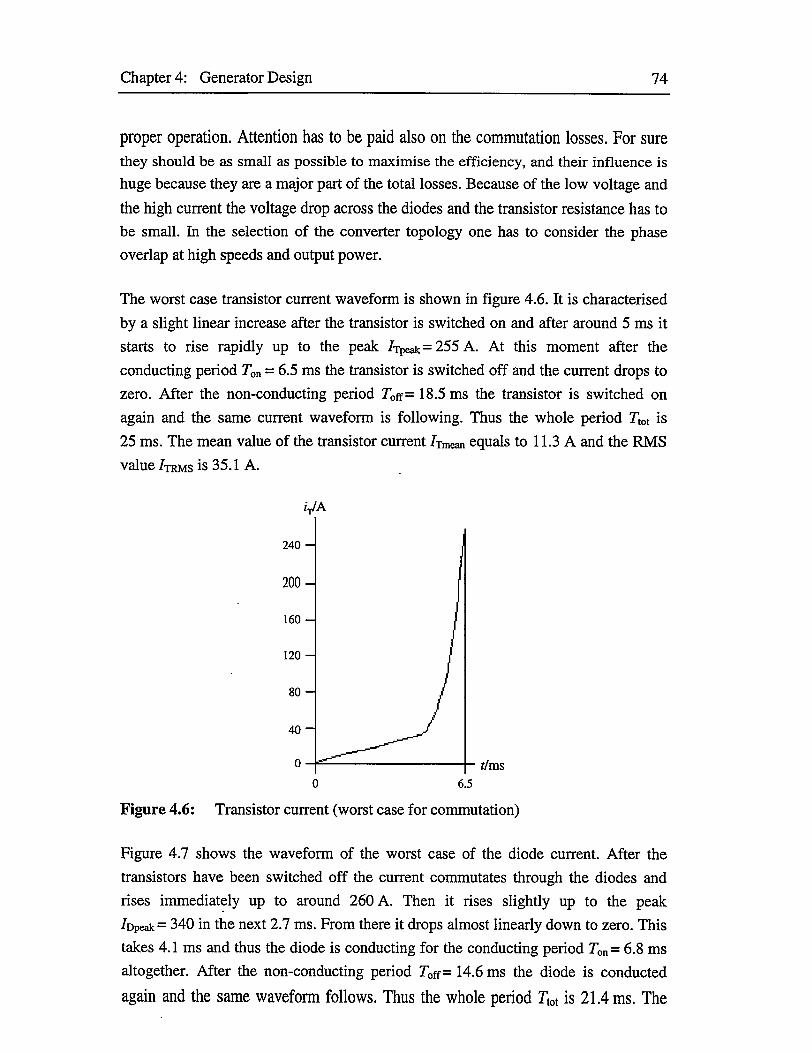
Chapter 4: Generator Design 74
proper operation. Attention has to be paid also on the commutation losses. For surethey should be as small as possible to maximise the efficiency, and their influence is huge because they are a major part of the total losses. Because of the low voltage and
the high current the voltage drop across the diodes and the transistor resistance has to
be small. In the selection of the converter topology one has to consider the phase
overlap at high speeds and output power.
The worst case transistor current waveform is shown in figure 4.6. It is characterised
by a slight linear increase after the transistor is switched on and after around 5 ms it
starts to rise rapidly up to the peak Apeak = 255 A. At this moment after the
conducting period Ton = 6.5 ms the transistor is switched off and the current drops to
zero. After the non-conducting period T0ff= 18.5 ms the transistor is switched on
again and the same current waveform is following. Thus the whole period Ttot is
25 ms. The mean value of the transistor current Amean equals to 11.3 A and the RMS
value Arms is 35.1 A.
VA
240 -
160 -
120 -
Figure 4.6: Transistor current (worst case for commutation)
Figure 4.7 shows the waveform of the worst case of the diode current. After the
transistors have been switched off the current commutates through the diodes and
rises immediately up to around 260 A. Then it rises slightly up to the peak
Apeak = 340 in the next 2.7 ms. From there it drops almost linearly down to zero. This
takes 4.1 ms and thus the diode is conducting for the conducting period Ton=6.8 ms
altogether. After the non-conducting period T0ff= 14.6 ms the diode is conducted
again and the same waveform follows. Thus the whole period Act is 21.4 ms. The
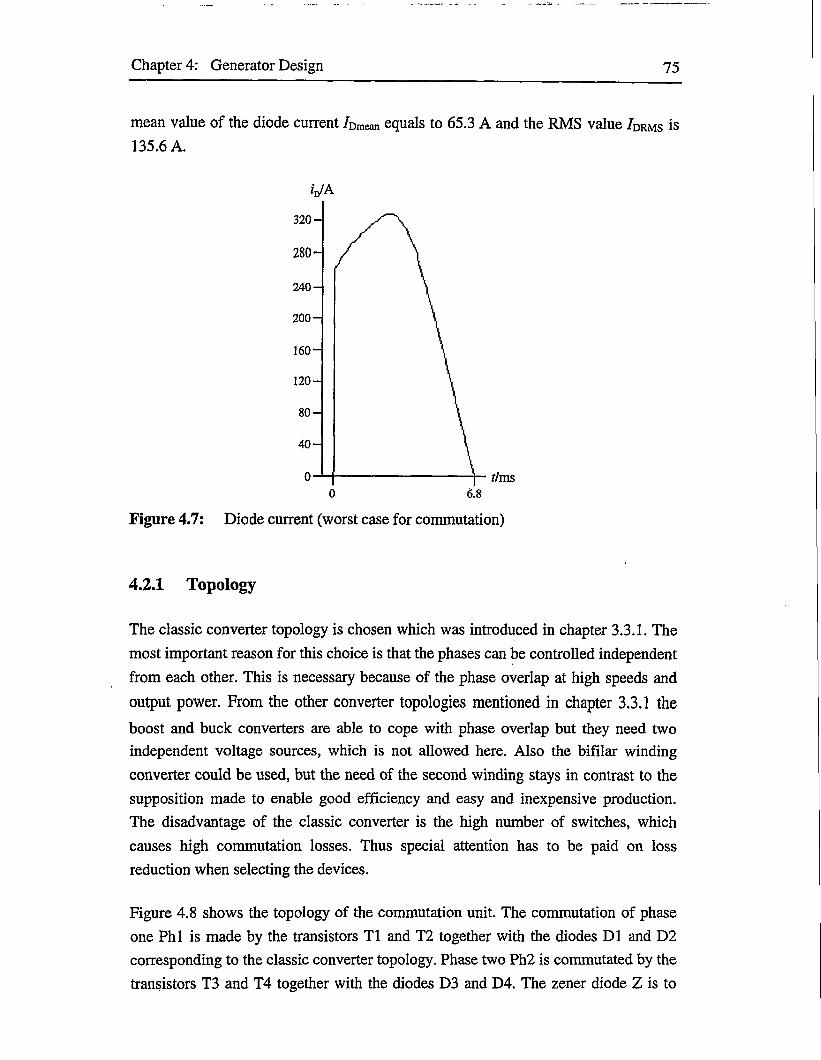
Chapter 4: Generator Design 75
mean value of the diode current /Dmean equals to 65.3 A and the RMS value /drms is
135.6 A.
VA
240-
200-
Figure 4.7: Diode current (worst case for commutation)
4.2.1 Topology
The classic converter topology is chosen which was introduced in chapter 3.3.1. The
most important reason for this choice is that the phases can be controlled independent
from each other. This is necessary because of the phase overlap at high speeds and
output power. From the other converter topologies mentioned in chapter 3.3.1 the
boost and buck converters are able to cope with phase overlap but they need two independent voltage sources, which is not allowed here. Also the bifilar winding
converter could be used, but the need of the second winding stays in contrast to the
supposition made to enable good efficiency and easy and inexpensive production.
The disadvantage of the classic converter is the high number of switches, which
causes high commutation losses. Thus special attention has to be paid on loss
reduction when selecting the devices.
Figure 4.8 shows the topology of the commutation unit. The commutation of phase
one Phi is made by the transistors T1 and T2 together with the diodes D1 and D2
corresponding to the classic converter topology. Phase two Ph2 is commutated by the
transistors T3 and T4 together with the diodes D3 and D4. The zener diode Z is to

Chapter 4: Generator Design 76
protect against voltage peaks which can appear by sudden changes of the load or
during the switch-off time of transistors because of parasitic inductances.
T3 iT1 i
Figure 4.8: Commutation unit topology
Generally, commutation units of switched reluctance machines need a capacitor filter
to smooth the low-frequency link current. This can be done by using a large
capacitor, but it can be renounced here because the battery U has a huge capacity
itself.
4.2.2 Transistors
Power MOSFETs are most suitable for this commutation unit because they can
switch the high currents. Another reason is the low driving power because they are
voltage controlled and thus only a small current is needed for the control. Also the
frequency range and the switching times fulfil the demands. The chosen transistor
type is the SEMITRANS M power MOSFET module SKM 101 AR which is
produced by SEMIKRON. It is an N-channel enhancement mode MOSFET. The data
sheet is included in reference [46] and the most important absolute maximum ratings
and characteristic values are summarised in table 4.5. In context with the table it
should be mentioned that the given switching times can be used for rough
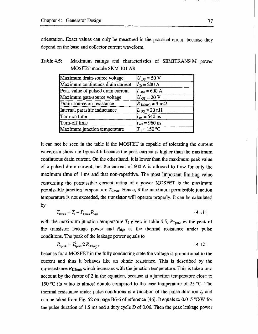
Chapter 4: Generator Design 77
orientation. Exact values can only be measured in the practical circuit because they
depend on the base and collector current waveform.
Table 4.5: Maximum ratings and characteristics of SEMITRANS M power
MOSFET module SKM 101 AR
Maximum drain-source voltage U DS = 50 VMaximum continuous drain current 7d = 200 APeak value of pulsed drain current /dm = 600 AMaximum gate-source voltage t/ gs = 20 VDrain-source on-resistance R DS(on) — 3 m£2Internal parasitic inductance L ds = 20 nHTurn-on time ron = 540 nsTurn-off time t off =960 nsMaximum junction temperature Tj=150°C
It can not be seen in the table if the MOSFET is capable of tolerating the current
waveform shown in figure 4.6 because the peak current is higher than the maximum
continuous drain current. On the other hand, it is lower than the maximum peak value
of a pulsed drain current, but the current of 600 A is allowed to flow for only the
maximum time of 1 ms and that non-repetitive. The most important limiting value
concerning the permissible current rating of a power MOSFET is the maximum permissible junction temperature Tcmax- Hence, if the maximum permissible junction
temperature is not exceeded, the transistor will operate properly. It can be calculated
byAmax = A ~ Apeak Ahjc (4.11)
with the maximum junction temperature 7j given in table 4.5, Prpeak as the peak of
the transistor leakage power and Pthjc as the thermal resistance under pulse
conditions. The peak of the leakage power equals to
Apeak = Apeak % A>S(on) ’ (412)
because for a MOSFET in the fully conducting state the voltage is proportional to the
current and thus it behaves like an ohmic resistance. This is described by the
on-resistance Pcston) which increases with the junction temperature. This is taken into
account by the factor of 2 in the equation, because at a junction temperature close to
150 °C its value is almost double compared to the case temperature of 25 °C. The
thermal resistance under pulse conditions is a function of the pulse duration rp and
can be taken from Fig. 52 on page B6-6 of reference [46]. It equals to 0.015 °C/W for
the pulse duration of 1.5 ms and a duty cycle D of 0.06. Then the peak leakage power
Chapter 4: Generator Design 78
is 390 W, and the maximum permissible junction temperature is 144 °C. Thus the
current can be tolerated if the junction temperature is kept below this limit.
The peak voltage which will arise from the current drop during turn-off of the
transistor has to be observed, as well. Its maximum value is not allowed to exceed
the maximum drain-source voltage Uus- Thus the inequation
us+L^ <yDS (4.13)dt (off)
must be fulfilled with U$ as the supply voltage and Lds as the internal parasitic
inductance. If the current is assumed to fall linearly the minimum allowed turn-off
time /off can be approximated to
AaS^Tpeak^off > uDS~us
(4.14)
and its value is around 145 ns. Compared with the turn-off time of 960 ns of the
transistor given in table 4.5 this value is much lower and thus it is insured that the
voltage peak caused by the internal parasitic inductance will not exceed the
maximum drain-source voltage. It should be mentioned that the parasitic inductances
of the connecting wires were neglected in this calculation. In addition the zener diode
is responsible for ensuring the safety of the transistors and diodes towards. high
frequency voltage peaks.
Concerning the commutation losses it is important that the transistor has a very low
on-resistance because it determines the losses. This is given by the chosen type,
because an on-resistance of 3 m£2 is very low for a MOSFET. Finally, it can be
concluded that the chosen MOSFET type fulfils the set demands.
4.2.3 Diodes
Schottky diodes are most suitable here because they can tolerate the high currents and
compared with other diodes they have a lower forward voltage drop, which effects
significantly on the commutation losses. Other reasons are the low capacitance,
absence of stored charge, zero switching losses and the fact that they can withstand
reverse voltage transients. The chosen diode type is the PBYR40045CT which is
produced by PHILIPS. It is a schottky barrier double rectifier diode. The data sheet is
included in reference [39] and the most important absolute maximum ratings and
characteristic values are summarised in table 4.6.
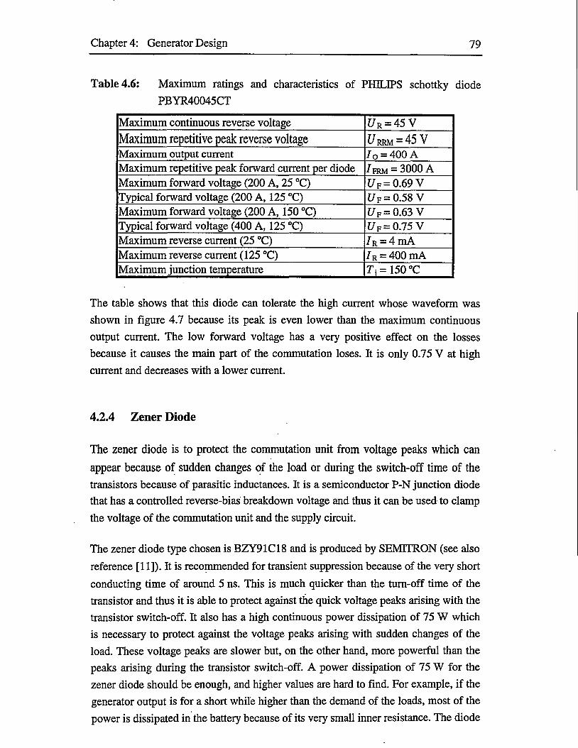
Chapter 4: Generator Design 79
Table 4.6: Maximum ratings and characteristics of PHILIPS schottky diode
PBYR40045CT
Maximum continuous reverse voltage C7r = 45 VMaximum repetitive peak reverse voltage U rrm = 45 VMaximum output current Io — 400 AMaximum repetitive peak forward current per diode 7FRM = 3000 AMaximum forward voltage (200 A, 25 °C) UF = 0.69 VTypical forward voltage (200 A, 125 °C) UF = 0.58 VMaximum forward voltage (200 A, 150 °C) UF = 0.63 VTypical forward voltage (400 A, 125 °C) I/F = 0.75 VMaximum reverse current (25 °C) 7R = 4mAMaximum reverse current (125 °C) 7r = 400 mAMaximum junction temperature T, = 150 °C
The table shows that this diode can tolerate the high current whose waveform was
shown in figure 4.7 because its peak is even lower than the maximum continuous
output current. The low forward voltage has a very positive effect on the losses
because it causes the main part of the commutation loses. It is only 0.75 V at high
current and decreases with a lower current.
4.2.4 Zener Diode
The zener diode is to protect the commutation unit from voltage peaks which can
appear because of sudden changes of the load or during the switch-off time of the
transistors because of parasitic inductances. It is a semiconductor P-N junction diode that has a controlled reverse-bias breakdown voltage and thus it can be used to clamp
the voltage of the commutation unit and the supply circuit.
The zener diode type chosen is BZY91C18 and is produced by SEMTTRON (see also
reference [11]). It is recommended for transient suppression because of the very short
conducting time of around 5 ns. This is much quicker than the turn-off time of the
transistor and thus it is able to protect against the quick voltage peaks arising with the
transistor switch-off. It also has a high continuous power dissipation of 75 W which
is necessary to protect against the voltage peaks arising with sudden changes of the
load. These voltage peaks are slower but, on the other hand, more powerful than the
peaks arising during the transistor switch-off. A power dissipation of 75 W for the
zener diode should be enough, and higher values are hard to find. For example, if the
generator output is for a short while higher than the demand of the loads, most of the
power is dissipated in the battery because of its very small inner resistance. The diode

Chapter 4: Generator Design 80
has to tolerate only the fast transients. This diode type has a break-down voltage of
18 V. This is a bit higher than the nominal output voltage of the generator of 14 V
but it is usual for transient suppression applications.
4.3 Control System
The control system has to keep the output voltage of the generator constant. The
voltage varies with changes of speed and load. Most suitable is a constant voltage of
14 V. This ensures charging of the battery and provides clearance to its gassing
voltage. The control system can be realised according to the structure shown in figure
3.24. The controller needs voltage and rotor position feedbacks.as input. It derives
the firing angles for the commutation from the voltage error and the speed according
to the control strategy. '
The optimum speed range of the generator is between 1,200 rpm and 12,000 rpm
which is 1.5 times the speed of internal combustion engines of motor vehicles. At
speeds under 1,200 rpm the transistor peak currents are becoming tremendous. Thus
the speed range has to be restricted to this minimum limit. Only small maximum
output power is supplied at speeds over 12,000 rpm but basically the generator is able
to operate above this limit.
The control strategy has to be chosen in a way that the transistor peak currents are
restricted to 250 A. This is necessary at low speeds. It will ensure the safe operation
of the commutation unit. Good efficiency and high maximum output power are also
demanding the choice of the control strategy. In addition the control strategy should
be as simple as possible to make the controller as inexpensive as possible. The
sensing should enable fast reaction and provide sufficient precision.
4.3.1 Control Strategy
The control strategy has to be chosen in the way that both firing angles are controlled.
This is necessary because otherwise the transistor peak currents at low speeds can not
be kept under 250 A. The dwell period has to be enlarged with an increase of speed
or load by changing the control modes. Because of the variation of both firing angles
the control modes can be used in their suitable speed range. This will affect positively on the efficiency.
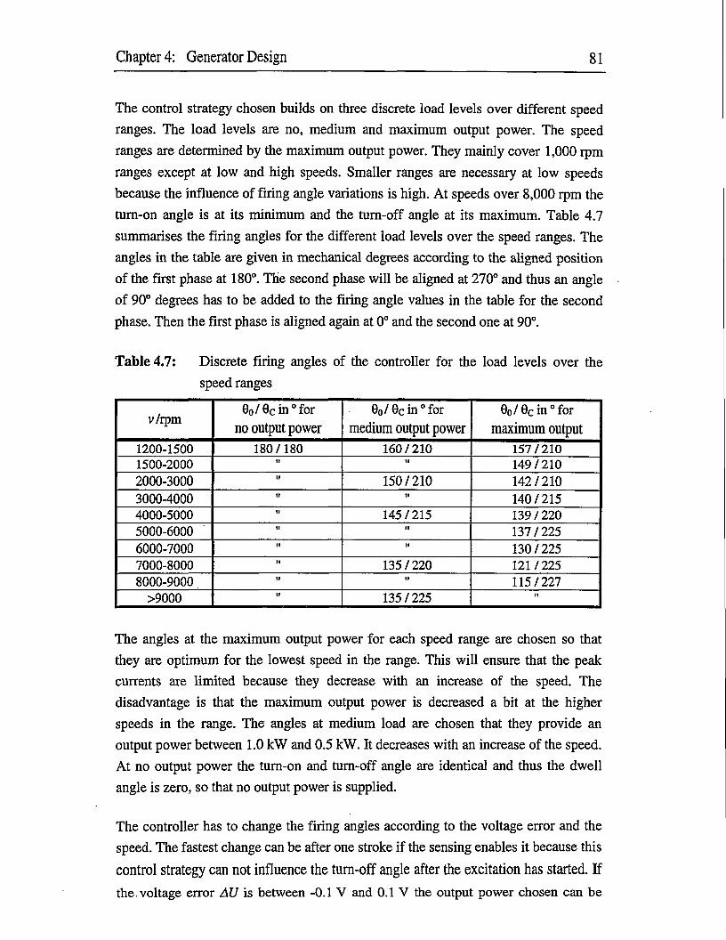
Chapter 4: Generator Design 81
The control strategy chosen builds on three discrete load levels over different speed
ranges. The load levels are no, medium and maximum output power. The speed
ranges are determined by the maximum output power. They mainly cover 1,000 rpm
ranges except at low and high speeds. Smaller ranges are necessary at low speeds
because the influence of firing angle variations is high. At speeds over 8,000 rpm the
turn-on angle is at its minimum and the turn-off angle at its maximum. Table 4.7
summarises the firing angles for the different load levels over the speed ranges. The
angles in the table are given in mechanical degrees according to the aligned position
of the first phase at 180°. The second phase will be aligned at 270° and thus an angle
of 90° degrees has to be added to the firing angle values in the table for the second
phase. Then the first phase is aligned again at 0° and the second one at 90°.
Table 4.7: Discrete firing angles of the controller for the load levels over the
speed ranges
v/rpm0O / 0c in ° for
no output power0o / 0c in ° for
medium output power0o / 0c in ° for
maximum output1200-1500 180/180 160/210 157/2101500-2000 it " 149/2102000-3000 ii 150/210 142/2103000-4000 ii 140/2154000-5000 u 145/215 139 / 2205000-6000 ii 137/2256000-7000 n 130/2257000-8000 n 135/220 121/2258000-9000 n 115/227
>9000 ii 135/225
The angles at the maximum output power for each speed range are chosen so that
they are optimum for the lowest speed in the range. This will ensure that the peak
currents are limited because they decrease with an increase of the speed. The
disadvantage is that the maximum output power is decreased a bit at the higher
speeds in the range. The angles at medium load are chosen that they provide an
output power between 1.0 kW and 0.5 kW. It decreases with an increase of the speed.
At no output power the turn-on and turn-off angle are identical and thus the dwell
angle is zero, so that no output power is supplied.
The controller has to change the firing angles according to the voltage error and the
speed. The fastest change can be after one stroke if the sensing enables it because this
control strategy can not influence the turn-off angle after the excitation has started. If
the. voltage error AU is between -0.1 V and 0.1 V the output power chosen can be
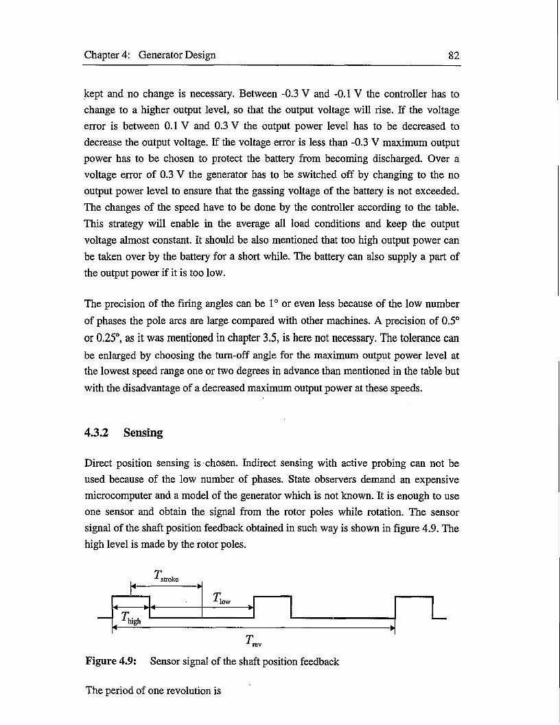
Chapter 4: Generator Design 82
kept and no change is necessary. Between -0.3 V and -0.1 V the controller has to
change to a higher output level, so that the output voltage will rise. If the voltage
error is between 0.1 V and 0.3 V the output power level has to be decreased to
decrease the output voltage. If the voltage error is less than -0.3 V maximum output
power has to be chosen to protect the battery from becoming discharged. Over a
voltage error of 0.3 V the generator has to be switched off by changing to the no
output power level to ensure that the gassing voltage of the battery is not exceeded.
The changes of the speed have to be done by the controller according to the table.
This strategy will enable in the average all load conditions and keep the output
voltage almost constant. It should be also mentioned that too high output power can
be taken over by the battery for a short while. The battery can also supply a part of
the output power if it is too low.
The precision of the firing angles can be 1° or even less because of the low number
of phases the pole arcs are large compared with other machines. A precision of 0.5°
or 0.25°, as it was mentioned in chapter 3.5, is here not necessary. The tolerance can
be enlarged by choosing the turn-off angle for the maximum output power level at the lowest speed range one or two degrees in advance than mentioned in the table but
with the disadvantage of a decreased maximum output power at these speeds.
4.3.2 Sensing
Direct position sensing is chosen. Indirect sensing with active probing can not be
used because of the low number of phases. State observers demand an expensive
microcomputer and a model of the generator which is not known. It is enough to use
one sensor and obtain the signal from the rotor poles while rotation. The sensor
signal of the shaft position feedback obtained in such way is shown in figure 4.9. The
high level is made by the rotor poles.
£■ stroke
— zhigh
■ low
Figure 4.9: Sensor signal of the shaft position feedback
The period of one revolution is

Chapter 4: Generator Design 83
T = 60(4.15)
the period of the high level is
the period of the low level is
and the excitation period is
60 9c-90 exc v 2tc
(4.16)
(4.17)
(4.18)
with v as the speed in rpm. The unit of the results is seconds. From equation (4.15)
the period of one stroke can be calculated by
T =■‘stroke N.(4.19)
strokes/rev
Table 4.8 shows the periods of time for different speeds. It can be seen that the stroke
period is shorter than the low level period. This has the disadvantage that the sensing
is too slow to enable the controller to react after each stroke. The delay will be
utmost two strokes. At speeds between 1,200 rpm and 1,500 rpm a delay of one
stroke can be realised if the sensor is placed in the right position because of the short
excitation period. The position for the sensor can be calculated by
0S = 2^1 - —j - 0O • (4.20)
and it is equal to 70.5°. A good position for the sensor then is 65° to provide some
clearance to the limit. This enables fast control after one stroke at the smallest speed
range, where it is most necessary, because of the high transistor peak currents and the
long period of one stroke. This should be fast enough for motor vehicle applications
because speed changes of the driving engine are quite small within the delay time of
the sensing because of the high inertia.
Table 4.8: The periods of time for different speeds
v/rpm 1200 1500 3000 6000 9000 12000T tot / ms 50 40 20 10 6.66 5T high / HIS 6.6 5.28 2.64 1.32 0.88 0.66T low / ms 18.4 14.72 7.36 3.68 2.45 1.84T stroke / mS 12.5 10 5 2.5 1.665 1.25T exc / ms 7.36 6.78 4.167 2.638 2.074 1.556

84
5 Simulation Results
The simulation results are obtained by simulations with the PC-SRD. They describe
the performance of the whole system including generator, commutation and control. The results are put together in a way that shows the system behaviour versus the
speed range and different load conditions. The speed range spans from 1,200 rpm to
12.000 rpm and the output power is varied in the four steps of 0.1 kW, 0.5 kW,
1.0 kW and the maximum output power. The maximum output power versus speed is
shown in figure 5.1. It is important to mention that the nominal output power of
1.5 kW is not reached at low and high speeds because it influences other
characteristic values and will be noticed in the following figures.
1600 T
1400 --
1200 --
1000 --
800 - •
600 - -
400 - -
200--
1000 2000 3000 4000 5000 6000 7000 8000 9000 10000 11000 12000
Figure 5.1: Maximum output power versus speed
The output power is kept constant or at its maximum to imitate the influence of the
controller. This is done by varying the firing angles. The turn-off angle is varied
throughout its range in 5° steps and the turn-on angle in 1° steps to reduce the
simulation effort with the PC-SRD. Otherwise many simulation runs have to be made
until the desired output power is obtained and different solutions are possible. At low
speeds and under maximum output power the turn-on angle is exceptionally varied in
0.5° steps, because the reaction of the generator on the control of the angles is more
sensible. The summary of the results is distinguished into input, output and inner
characteristics, efficiency and losses. The figures are derived from the tables included
in Appendix D. Also the waveforms of some dimensions are presented for different
speeds. The speeds are chosen to 1,200 rpm, 4,500 rpm and 9,000 rpm to cover the whole range.

Chapter 5: Simulation Results 85
5.1 Input
The generator input consists of mechanical and electrical input. Mechanical input is
the shaft torque provided by the driving machine. The shaft power corresponds with
it. Electrical input is the excitation current supplied by the battery. It builds up the
magnetic field.
The average shaft torque versus speed is shown in figure 5.2 for the four load
conditions. It can be seen that it decreases significantly with the speed and depends
also on the load. Less output power has to be provided with lower load and thus the
mechanical input decreases, because only the mechanical input is converted to output
power. The shaft torque decreasing with the speed can be explained by the equation
7'shaft CO = f shaft together with figure 5.4. As the figure shows, the shaft power is
almost constant over the speed range and thus the shaft torque indirectly proportional
to the angular velocity. This explains the curve shape in figure 5.2.
T Shaft/Nm14.0 T
13.0-
12.0" —max (1.5 kW)11.0 - —1.0 kW10.0- —0.5 kW9.0-
— 0.1 kW
7.0--6.0 - -
5.0-
4.0 - -3.0-2.0-
1000 2000 3000 4000 5000 6000 7000 8000 9000 10000 11000 12000
Figure 5.2: Average shaft torque versus speed for different load conditions
The shaft torque at the maximum load is partly influenced by the maximum output
power decreased at low and high speed. At low speeds it rises with the speed until the
nominal output power is supplied. At this point the shaft torque is at its maximum.
Also at high speeds it is lower than expected for the same reason. The curve differs a
bit from the ideal shape at low speeds because of the sensitivity of the generator
related to the control. The firing angles are not chosen accurately enough because
otherwise, as already mentioned, the simulation effort would be tremendous. This can

Chapter 5: Simulation Results 86
be, and sometimes even better, noticed from the other figures included in this
chapter.
Besides the average shaft torque, the waveform of the torque is of interest. It is
shown in figure 5.3 for three speeds at the maximum output power. Actually, the
total torque of both phases and the torque of just one phase is included, but in parts
(a) and (b) it can not be noticed because they overlap totally. This can be explained
by the total independence of the phases at these speeds. Thus the waveforms of single
phases are just added to the total waveform. They do not affect each other. The
difference can be seen only in part (c) of the figure. The torque of single phases
intersects and thus the total waveform does not overlap.
The figure shows that the torque is pulsating and has quite high peaks. With an
increase of the speed the peak is getting sharper but its maximum value is decreasing.
The comparison of the peak value with the average torque shows that their ratio is
increasing with the speed from around 2.5 up to 9.5. Compared with the. output
torque produced by the internal combustion engine of a motor vehicle for driving, the
average torque and the peak torque are small. Thus the pulsating torque will cause
just a small ripple and is not a problem in this kind of application.
The peak is also a bit postponed because of the postponed turn-off angle. The
turn-off angles for the different speeds are (a) 210°, (b) 220° and (c) 227°. It can be
seen that the torque is taken over already before the turn-off angle. It is stored in the
field energy at first because it can not be delivered to the supply before the turn-off of
the transistors. At 9,000 rpm the waveform for a single phase shows a positive torque
which is produced by the supply current because of the turn-on angle far before the
aligned position caused by the long dwell control mode. This positive torque overlaps
with the negative torque of the other phase. It is taken straight over by it and thus it is
not wasted.
The average shaft power is shown in figure 5.4. It is constant over the speed range for
a constant output. At the maximum output power it is not constant because of the not
always reached nominal output power. The waveform has almost the same shape
than the waveform of maximum output power. This quite similar behaviour of input
and output points towards almost constant total losses versus speed and load.
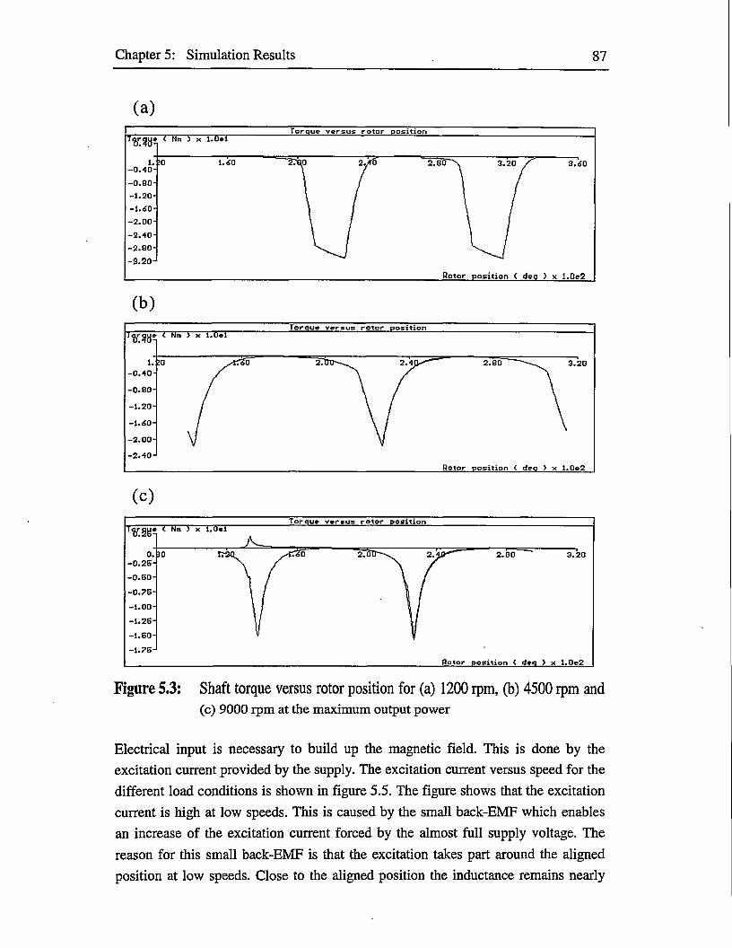
Chapter 5: Simulation Results 87
(a)Torque versus rotor position
< Nm ) x l.Uel
1.-0.40-
-0.80-
-1.20-
-1.40-
-2.00-
-2.40-
-2.80-
-3.20-
10 1.60 3.60
Rotor position ( dea ) x 1.0e2
(b)
Torque versus rotor position< Nm > x l.Oel
1.-0.40-
-0.80-
-1.20-
-1.40-
-2.00-
-2.40-
!0 2 --------------------------------------- 2"80
Rotor position < dea > x 1.0e2
(C)
Torque versus rotor position< Nm > x l.Oel
0.-0.25-
-0.50-
-0.75-
-1.00-
-1.26-
-1.60-
-1.75-
10 1.00—2.00 3.20
Rotor position ( deq > x 1.0e2
Figure 5.3: Shaft torque versus rotor position for (a) 1200 rpm, (b) 4500 rpm and(c) 9000 rpm at the maximum output power
Electrical input is necessary to build up the magnetic field. This is done by the excitation current provided by the supply. The excitation current versus speed for the
different load conditions is shown in figure 5.5. The figure shows that the excitation
current is high at low speeds. This is caused by the small back-EMF which enables
an increase of the excitation current forced by the almost full supply voltage. The
reason for this small back-EMF is that the excitation takes part around the aligned
position at low speeds. Close to the aligned position the inductance remains nearly

Chapter 5: Simulation Results 88
constant and only a changing inductance generates a sufficient back-EMF which
consumes part of the supply voltage.
P shaft/W — max (1.5 kW)2000 T 1.0 kW
0.5 kW1800--0.1 kW
1600 - -
1400 --
1200 - -
1000--
800 -
600 -
400 - -
200--
1000 2000 3000 4000 5000 6000 7000 8000 9000 10000 11000 12000
Figure 5.4: Average shaft power versus speed for different load conditions
—max (1.5 kW) —1.0 kW —0.5 kW — 0.1 kW
1000 2000 3000 4000 5000 6000 7000 8000 9000 10000 11000 12000
Figure 5.5: Excitation current versus speed for different load conditions
At medium speeds the excitation current is at its minimum, because the back-EMF is
bigger because of the advanced beginning of the excitation. Another main influence
on the excitation current besides the back-EMF is the control mode, and the normal
control mode is still used at medium speeds. The advantage of the normal control
mode is that only a very small positive torque is produced and its influence on the
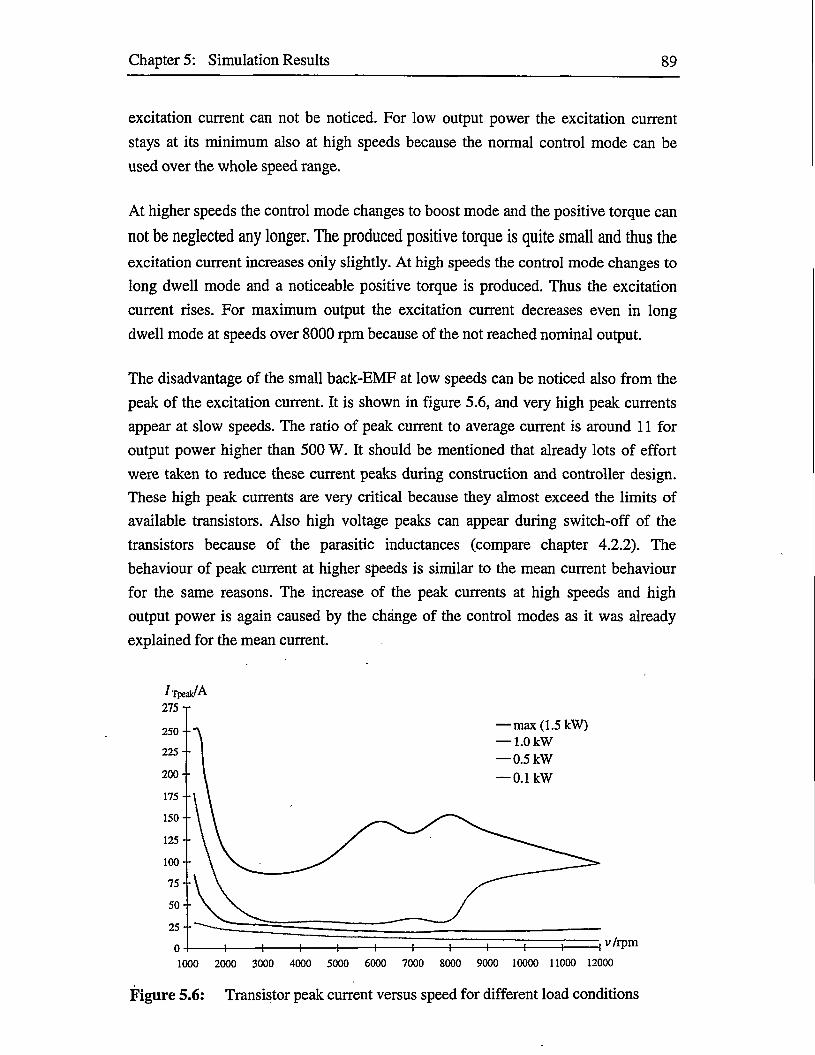
Chapter 5: Simulation Results 89
excitation current can not be noticed. For low output power the excitation current
stays at its minimum also at high speeds because the normal control mode can be
used over the whole speed range.
At higher speeds the control mode changes to boost mode and the positive torque can
not be neglected any longer. The produced positive torque is quite small and thus the
excitation current increases only slightly. At high speeds the control mode changes to
long dwell mode and a noticeable positive torque is produced. Thus the excitation
current rises. For maximum output the excitation current decreases even in long
dwell mode at speeds over 8000 rpm because of the not reached nominal output.
The disadvantage of the small back-EMF at low speeds can be noticed also from the
peak of the excitation current. It is shown in figure 5.6, and very high peak currents
appear at slow speeds. The ratio of peak current to average current is around 11 for
output power higher than 500 W. It should be mentioned that already lots of effort
were taken to reduce these current peaks during construction and controller design. These high peak currents are very critical because they almost exceed the limits of
available transistors. Also high voltage peaks can appear during switch-off of the
transistors because of the parasitic inductances (compare chapter 4.2.2). The
behaviour of peak current at higher speeds is similar to the mean current behaviour
for the same reasons. The increase of the peak currents at high speeds and high
output power is again caused by the change of the control modes as it was already
explained for the mean current.
/rpeak/A
—max (1.5 —1.0 kW —0.5 kW — 0.1 kW
250 --
225 -
200-
175 -
150--
125 --
100-
1000 2000 3000 4000 5000 6000 7000 8000 9000 10000 11000 12000
Figure 5.6: Transistor peak current versus speed for different load conditions

Chapter 5: Simulation Results 90
5.2 Output
Output is provided by the DC link current. The current is directly proportional to the
output power according to equation Pcu = kc U because of the constant controlled
voltage. Thus it is not shown here because its behaviour versus speed and load is equal to the output power behaviour which is shown in figure 5.7. Of interest are
mainly just the nominal output current of 107 A and the waveforms shown later.
PoutAV —max (1.5 kW)1.0 kW1600 T0.5 kW
1400 -- — 0.1 kW
1200 - -
1000--
800 - ■
600 - -
400 - ■
200--
1000 2000 3000 4000 5000 6000 7000 8000 9000 10000 11000 12000
Figure 5.7: Output power versus speed for different load conditions
The output power is kept constant according to the demands of the load. Above the
power of 1 kW it can not be kept constant over the whole speed range because for
some speeds the maximum output power is then reached. From the curve of
maximum output power it can be seen that the nominal output power can not be
reached over the whole speed range. At low speeds up to 1,400 rpm it has to be
reduced for limiting the excitation peak current. At speeds over 8,000 rpm the output
power is decreasing because the excitation period is too short to enable a sufficient
excitation and it can not be extended above the already reached maximum. In these
cases the battery has to provide the power if an output higher than the maximum is
demanded.
For the use in motor vehicles it is not momentous that the maximum output power is
lower than the nominal output power at these speeds. An output power of 1.25 kW at
the speed of 1,200 is already quite high and at least higher than for alternators. If the
battery gets partly discharged while the combustion engine is at idling speed, it can
be charged again at a higher speeds during driving. The reduced output power at high
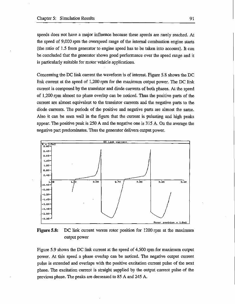
Chapter 5: Simulation Results 91
speeds does not have a major influence because these speeds are rarely reached. At
the speed of 9,000 rpm the overspeed range of the internal combustion engine starts
(the ratio of 1.5 from generator to engine speed has to be taken into account). It can
be concluded that the generator shows good performance over the speed range and it
is particularly suitable for motor vehicle applications.
Concerning the DC link current the waveform is of interest. Figure 5.8 shows the DC
link current at the speed of 1,200 rpm for the maximum output power. The DC link
current is composed by the transistor and diode currents of both phases. At the speed
of 1,200 rpm almost no phase overlap can be noticed. Thus the positive parts of the
current are almost equivalent to the transistor currents and the negative parts to the
diode currents. The periods of the positive and negative parts are almost the same.
Also it can be seen well in the figure that the current is pulsating and high peaks
appear. The positive peak is 250 A and the negative one is 315 A. On the average the
negative part predominates. Thus the generator delivers output power.
DC Link current
2.00-
1.20-0.80-
2.00 2.401. >0 2.80-0.40--0.80-
-2.00-
Rotor position x 1.0*2
Figure 5.8: DC link current versus rotor position for 1200 rpm at the maximum
output power
Figure 5.9 shows the DC link current at the speed of 4,500 rpm for maximum output
power. At this speed a phase overlap can be noticed. The negative output current
pulse is extended and overlaps with the positive excitation current pulse of the next
phase. The excitation current is straight supplied by the output current pulse of the
previous phase. The peaks are decreased to 85 A and 245 A.

Chapter 5: Simulation Results 92
DC Link currentfT x 1.0e2
0.40-
2.40 2.80 3.201. >0
-0.40-
-0.80-
-1.20-
-2.00-
-2.20-
Rotor position x 1.0o2
Figure 5.9: DC link current versus rotor position for 4500 rpm at the maximum
output power
Figure 5.10 shows the DC link current at a speed of 9,000 rpm for maximum output
power. At this speed the phase currents overlap completely. The turn-on of the
second phase is at an angle of 115° and the first phase is turned off later at an angle of
137°. The positive current pulse is very short now because the negative output current pulse is still more extended and supplies straight the excitation of the other phase. The positive peak is increased again up to 135 A because of the change of the control
mode to long dwell mode. The negative peak is more decreased down to 195 A.
DC Link currentA x 1.01
1.40-
1.20-1.00-0.80-
0.40-
0.20-
1.20 2.00 2.40 2.80 3.20
-0.40-
-1.00--1.20-
-1.80-
Potor positi' 1.0o2
Figure 5.10: DC link current versus rotor position for 9000 rpm at the maximum
output power

Chapter 5: Simulation Results 93
From the comparison of the figures of the DC link current waveforms it can be
concluded that the pulse of the negative output current is extended with the speed.
Also its peak value decreases and the peak appears earlier after commutation.
Respectively the positive pulse is shortened at higher speeds. Its peak value is at the
maximum at low speeds, medium at medium speeds and increases again at high
speeds. The rising time of the current up to the peak increases with higher speeds.
5.3 Phase Current
Figure 5.11 presents the average phase current. It is almost constant versus speed at
not maximum output power. This shows that the losses are almost constant versusspeed because the output current is constant, too. At 1 kW output power the phase
current increases a bit at high speeds. This is caused by the higher excitation current
because of the changed control mode. The phase current at maximum output power is
influenced by the not always reached maximum output power. Thus it decreases at high speeds and is also not at its maximum at low speeds. The increase at speeds
from 5,000 rpm to 8,000 rpm is caused by the higher excitation current for the same
reason than at the lower output power. The phase current is higher at low speeds for
all load conditions because of the very high excitation current.
—max (1.5 kW) —1.0 kW —0.5 kW — 0.1 kW
1000 2000 3000 4000 5000 6000 7000 8000 9000 10000 11000 12000
Figure 5.11: Phase current versus speed for different load conditions
The phase peak current is shown in figure 5.12. It equals the peak of the diode
current. The equality with the diode peak current is obvious because the diode peak
current is much higher than the transistor peak current. The phase peak current has
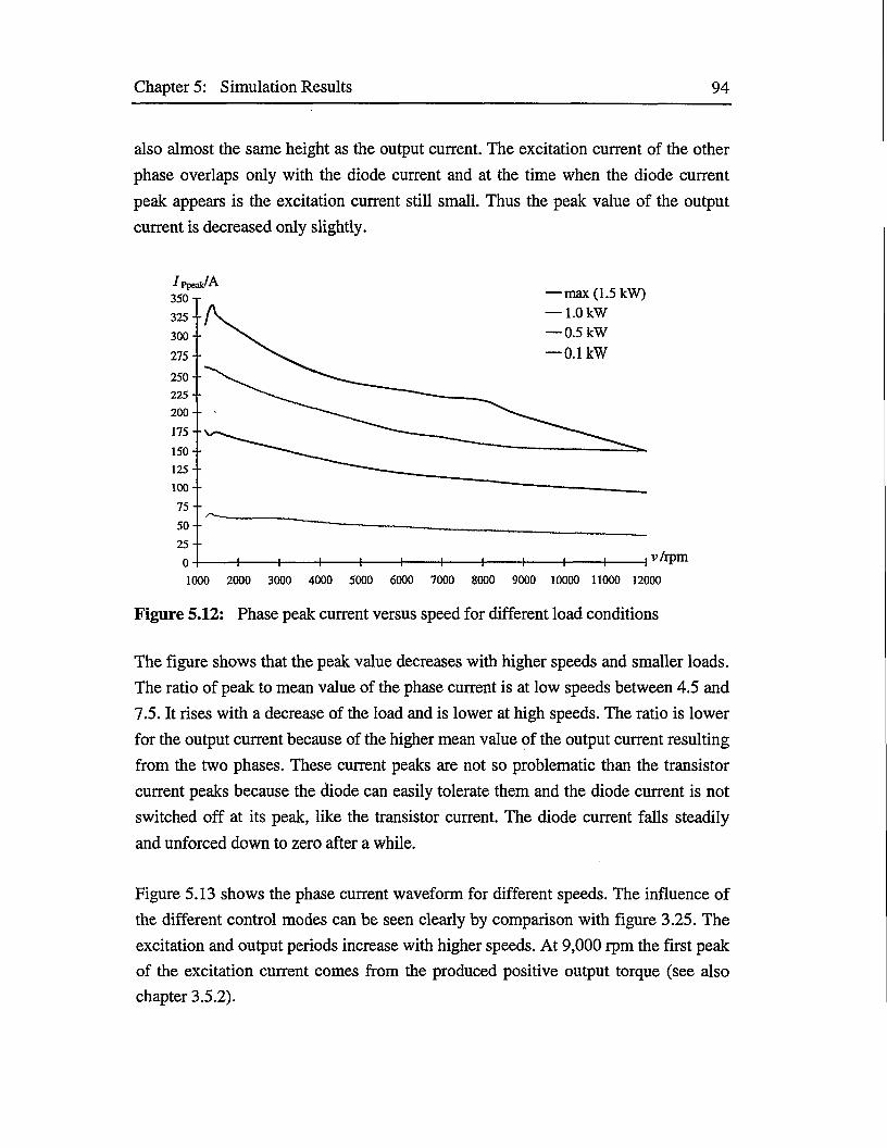
Chapter 5: Simulation Results 94
also almost the same height as the output current. The excitation current of the other
phase overlaps only with the diode current and at the time when the diode current
peak appears is the excitation current still small. Thus the peak value of the output
current is decreased only slightly.
—max (1.5 kW)350 T1.0 kW325 --0.5 kW300 -0.1 kW275 --
250 --225 --200-- ■
175--
150 - -125 --100-
1000 2000 3000 4000 5000 6000 7000 8000 9000 10000 11000 12000
Figure 5.12: Phase peak current versus speed for different load conditions
The figure shows that the peak value decreases with higher speeds and smaller loads.
The ratio of peak to mean value of the phase current is at low speeds between 4.5 and
7.5. It rises with a decrease of the load and is lower at high speeds. The ratio is lower
for the output current because of the higher mean value of the output current resulting
from the two phases. These current peaks are not so problematic than the transistor
current peaks because the diode can easily tolerate them and the diode current is not
switched off at its peak, like the transistor current. The diode current falls steadily
and unforced down to zero after a while.
Figure 5.13 shows the phase current waveform for different speeds. The influence of
the different control modes can be seen clearly by comparison with figure 3.25. The
excitation and output periods increase with higher speeds. At 9,000 rpm the first peak
of the excitation current comes from the produced positive output torque (see also
chapter 3.5.2).
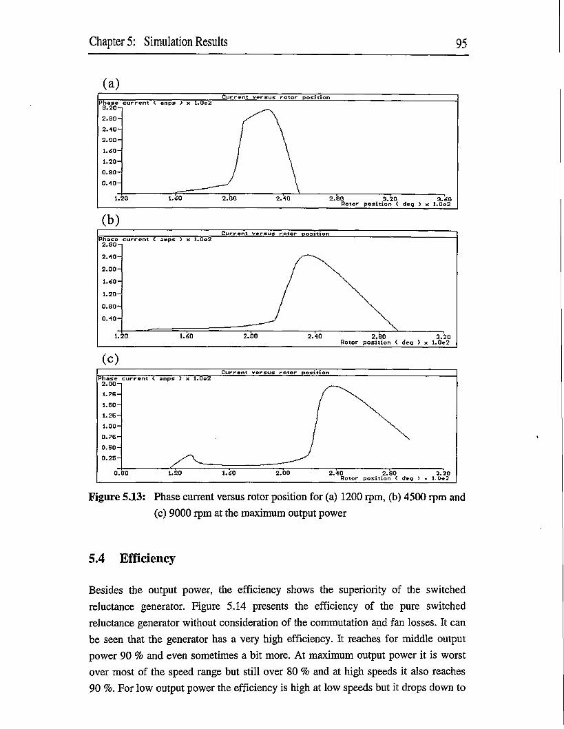
Chapter 5: Simulation Results 95
(a)Current versus rotor position
Phase ips ) x 1.0e23.20-]
2.80-
2.40-
2.00-
1.20-0.80-
2.80Rotor position < deg > x 1.0e2
(b)Current versus rotor position
Phase current < amps > x 1.0e22.80-1
2.00-
1.20-
0.80-
2.80 3.20Rotor position < deg > x 1.0e2
(c)Current versus rotor position
Phase current ( amps ) x 1.0e22.00-1
1.50-
1.25-
1.00-0.76-
0.26-
2.000.80 2.40 2.80____ 3.20Rotor position ( deg > • t. 0e2
Figure 5.13: Phase current versus rotor position for (a) 1200 rpm, (b) 4500 rpm and
(c) 9000 rpm at the maximum output power
5.4 Efficiency
Besides the output power, the efficiency shows the superiority of the switched
reluctance generator. Figure 5.14 presents the efficiency of the pure switched
reluctance generator without consideration of the commutation and fan losses. It can
be seen that the generator has a very high efficiency. It reaches for middle output
power 90 % and even sometimes a bit more. At maximum output power it is worst
over most of the speed range but still over 80 % and at high speeds it also reaches
90 %. For low output power the efficiency is high at low speeds but it drops down to
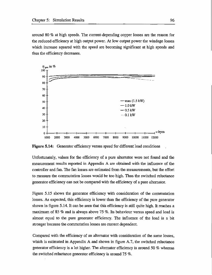
Chapter 5: Simulation Results 96
around 80 % at high speeds. The current-depending copper losses are the reason for
the reduced efficiency at high output power. At low output power the windage losses
which increase squared with the speed are becoming significant at high speeds and
thus the efficiency decreases.
h gen in100 T
—max (1.5 kW) —1.0 kW —0.5 kW - 0.1 kW
1000 2000 3000 4000 5000 6000 7000 8000 9000 10000 11000 12000
Figure 5.14: Generator efficiency versus speed for different load conditions
Unfortunately, values for the efficiency of a pure alternator were not found and the
measurement results reported in Appendix A are obtained with the influence of the
controller and fan. The fan losses are estimated from the measurements, but the effort
to measure the commutation losses would be too high. Thus the switched reluctance
generator efficiency can not be compared with the efficiency of a pure alternator.
Figure 5.15 shows the generator efficiency with consideration of the commutation
losses. As expected, this efficiency is lower than the efficiency of the pure generator
shown in figure 5.14. It can be seen that this efficiency is still quite high. It reaches a
maximum of 85 % and is always above 75 %. Its behaviour versus speed and load is
almost equal to the pure generator efficiency. The influence of the load is a bit
stronger because the commutation losses are current dependent.
Compared with the efficiency of an alternator with consideration of the same losses,
which is estimated in Appendix A and shown in figure A.7, the switched reluctance
generator efficiency is a lot higher. The alternator efficiency is around 50 % whereas
the switched reluctance generator efficiency is around 75 %.
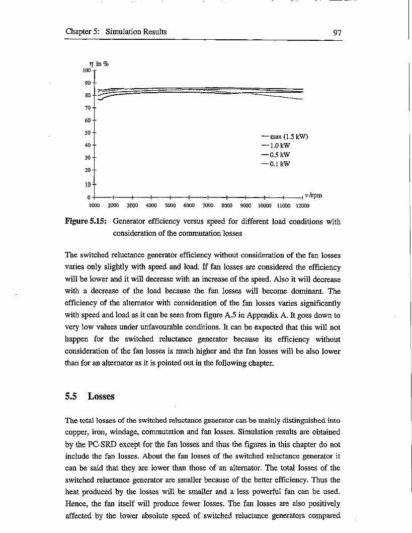
Chapter 5: Simulation Results 97
77 in %100 T
—max (1.5 kW) —1.0 kW —0.5 kW — 0.1 kW
1000 2000 3000 4000 5000 6000 7000 8000 9000 10000 11000 12000
Figure 5.15: Generator efficiency versus speed for different load conditions with
consideration of the commutation losses
The switched reluctance generator efficiency without consideration of the fan losses
varies only slightly with speed and load. If fan losses are considered the efficiency
will be lower and it will decrease with an increase of the speed. Also it will decrease
with a decrease of the load because the fan losses will become dominant. The
efficiency of the alternator with consideration of the fan losses varies significantly
with speed and load as it can be seen from figure A.5 in Appendix A. It goes down to
very low values under unfavourable conditions. It can be expected that this will not
happen for the switched reluctance generator because its efficiency without
consideration of the fan losses is much higher and the fan losses will be also lower
than for an alternator as it is pointed out in the following chapter.
5.5 Losses
The total losses of the switched reluctance generator can be mainly distinguished into
copper, iron, windage, commutation and fan losses. Simulation results are obtained
by the PC-SRD except for the fan losses and thus the figures in this chapter do not include the fan losses. About the fan losses of the switched reluctance generator it
can be said that they are lower than those of an alternator. The total losses of the
switched reluctance generator are smaller because of the better efficiency. Thus the
heat produced by the losses will be smaller and a less powerful fan can be used.
Hence, the fan itself will produce fewer losses. The fan losses are also positively
affected by the lower absolute speed of switched reluctance generators compared
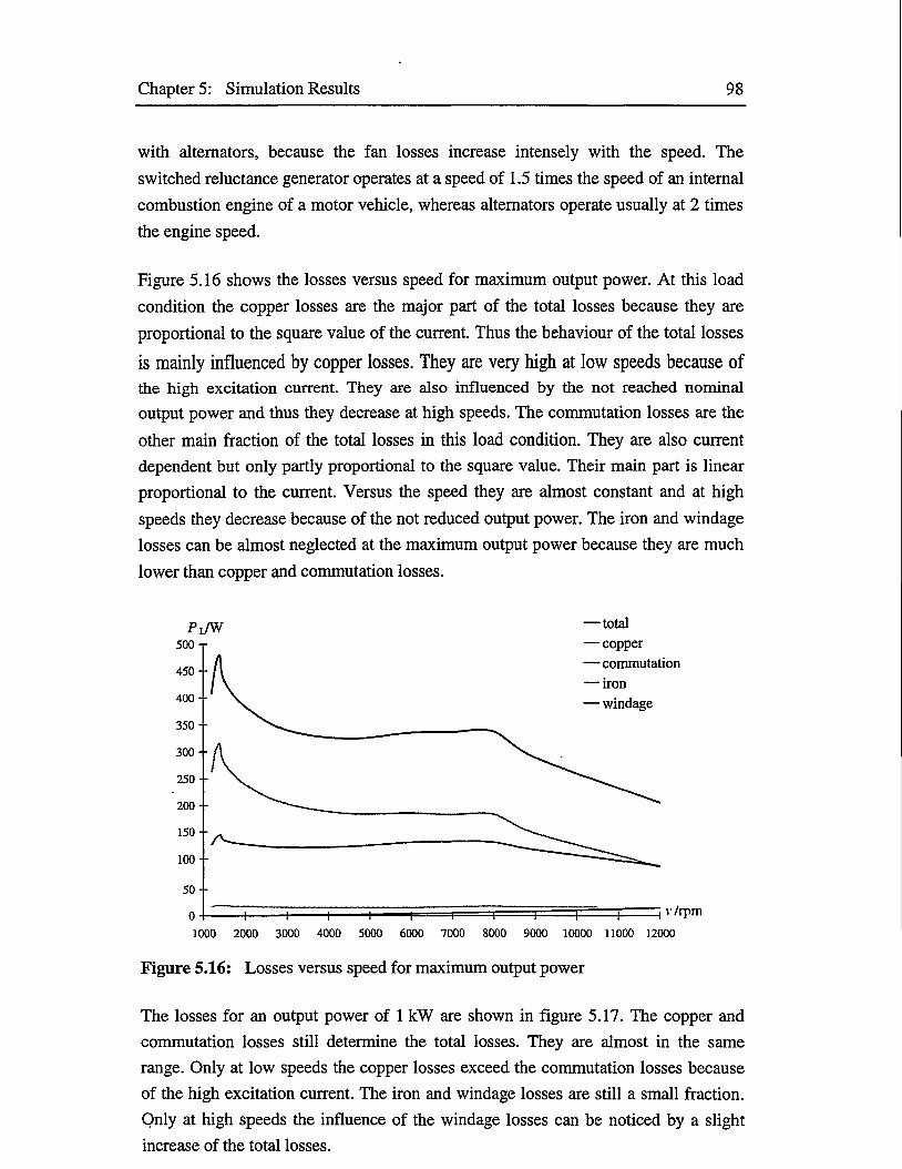
Chapter 5: Simulation Results 98
with alternators, because the fan losses increase intensely with the speed. The
switched reluctance generator operates at a speed of 1.5 times the speed of an internal
combustion engine of a motor vehicle, whereas alternators operate usually at 2 times
the engine speed.
Figure 5.16 shows the losses versus speed for maximum output power. At this load
condition the copper losses are the major part of the total losses because they are
proportional to the square value of the current. Thus the behaviour of the total losses
is mainly influenced by copper losses. They are very high at low speeds because ofthe high excitation current. They are also influenced by the not reached nominal output power and thus they decrease at high speeds. The commutation losses are the
other main fraction of the total losses in this load condition. They are also current dependent but only partly proportional to the square value. Their main part is linear
proportional to the current. Versus the speed they are almost constant and at high
speeds they decrease because of the not reduced output power. The iron and windage
losses can be almost neglected at the maximum output power because they are much
lower than copper and commutation losses.
P l/w —total500 T — copper
—commutation— iron— windage
450-
400 * •
350 - ■
300 -
250 - -
200--
150-
100-
1000 2000 3000 4000 5000 6000 7000 8000 9000 10000 11000 12000
Figure 5.16: Losses versus speed for maximum output power
The losses for an output power of 1 kW are shown in figure 5.17. The copper and
commutation losses still determine the total losses. They are almost in the same
range. Only at low speeds the copper losses exceed the commutation losses because
of the high excitation current. The iron and windage losses are still a small fraction.
Only at high speeds the influence of the windage losses can be noticed by a slight
increase of the total losses.
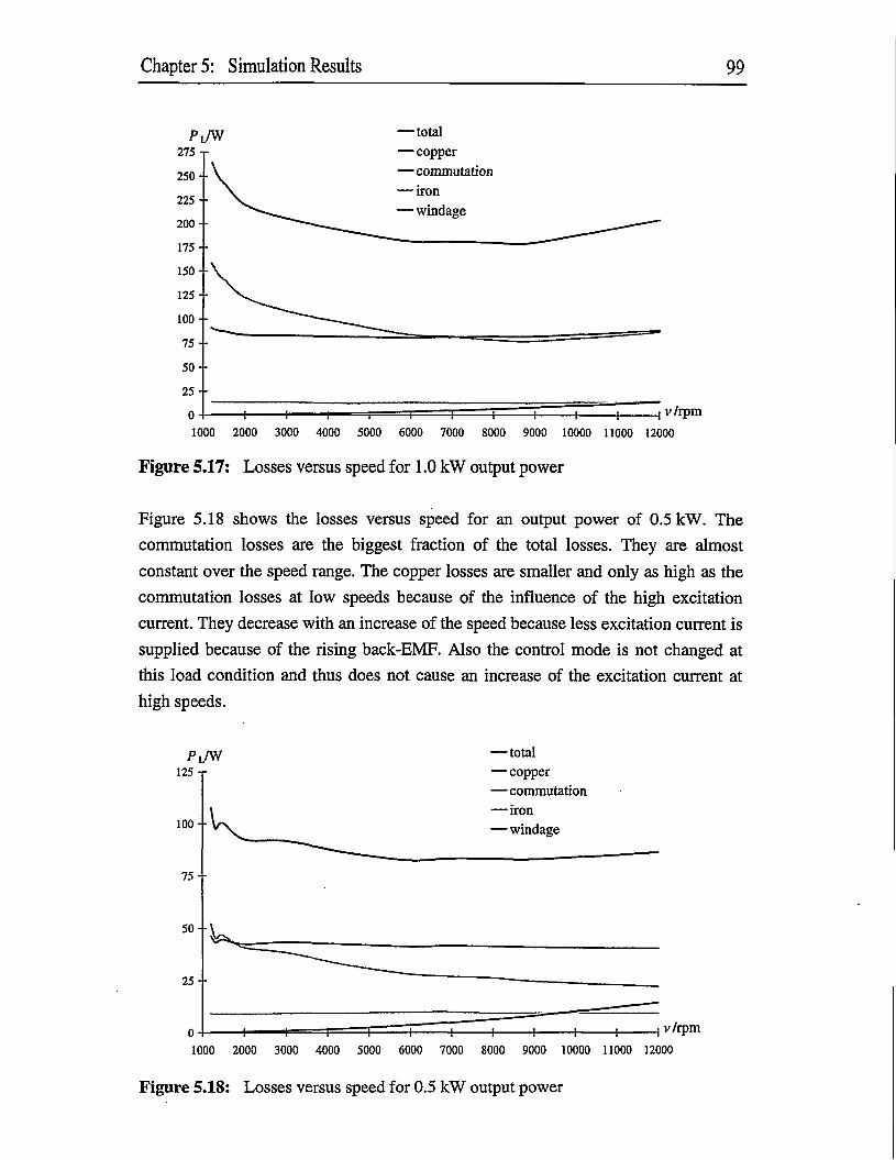
Chapter 5: Simulation Results 99
PJW —total275 T —copper
—commutation— iron— windage
250 -
225 --
200-
175 -
150 -
125 -
100 -
1000 2000 3000 4000 5000 6000 7000 8000 9000 10000 11000 12000
Figure 5.17: Losses versus speed for 1.0 kW output power
Figure 5.18 shows the losses versus speed for an output power of 0.5 kW. The
commutation losses are the biggest fraction of the total losses. They are almost
constant over the speed range. The copper losses are smaller and only as high as the
commutation losses at low speeds because of the influence of the high excitation
current. They decrease with an increase of the speed because less excitation current is
supplied because of the rising back-EMF. Also the control mode is not changed at
this load condition and thus does not cause an increase of the excitation current at
high speeds.
PlAV —total125 T —copper
—commutation —iron —windage100 -
1000 2000 3000 4000 5000 6000 7000 8000 9000 10000 11000 12000
Figure 5.18: Losses versus speed for 0.5 kW output power
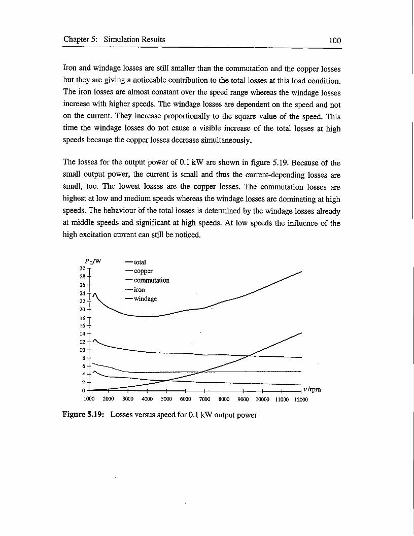
Chapter 5: Simulation Results 100
Iron and windage losses are still smaller than the commutation and the copper losses
but they are giving a noticeable contribution to the total losses at this load condition.
The iron losses are almost constant over the speed range whereas the windage losses
increase with higher speeds. The windage losses are dependent on the speed and not
on the current. They increase proportionally to the square value of the speed. This
time the windage losses do not cause a visible increase of the total losses at high
speeds because the copper losses decrease simultaneously.
The losses for the output power of 0.1 kW are shown in figure 5.19. Because of the
small output power, the current is small and thus the current-depending losses are
small, too. The lowest losses are the copper losses. The commutation losses are
highest at low and medium speeds whereas the windage losses are dominating at high
speeds. The behaviour of the total losses is determined by the windage losses already
at middle speeds and significant at high speeds. At low speeds the influence of the
high excitation current can still be noticed.
•Pl/W —total— copper—commutation— iron— windage22--
1000 2000 3000 4000 5000 6000 7000 8000 9000 10000 11000 12000
Figure 5.19: Losses versus speed for 0.1 kW output power
101
6 Conclusion and Prospects
The task of this work has been to design a low voltage switched reluctance generator
for variable speed applications. As appropriate and main field of application the
generator is considered to be used for the on-board power supply in motor vehicles.
As basis for the designing process the principle and theory of switched reluctance
generators have been worked out. The construction and the commutation unit are
designed in detail. The strategy for the realisation of the control system is given. The
performance of the whole system is presented by the obtained simulation results. An
overview, of the existing technology for variable speed applications has been
presented to complete the expositions of the topic.
The switched reluctance generator, which has been designed in this work, fulfils the
required demands, like high output power and efficiency. It is capable of supplying a
nominal output power of 1.5 kW and the efficiency is above 75 %. These values are
reached almost over the whole speed range and the efficiency varies only slightly
over the output power range. The performance of the generator exceeds the
characteristics of the nowadays alternator technology used. The better efficiency will
affect positively on the fuel consumption of motor vehicles.
Prospective work could be to complete the design of the control system based on the
recommended strategy. The next step then would be to build and investigate a
prototype generator.

102
7 References
[1] Arkadan, A.A.; Kielgas, B.W.: “Switched Reluctance Motor Drive Systems Dynamic Performance Prediction and Experimental Verification”. IEEE Transactions on Energy Conversion, Vol. 9, No. 1,1994, pp. 36-44.
[2] Arkadan, A.A.; Kielgas, B.W.: “Switched Reluctance Motor Drive Systems Dynamic Performance Prediction Under Internal and External Fault Conditions”. IEEE Transactions on Energy Conversion, Vol. 9, No. 1, 1994, pp. 45-52.
[3] Becerra, R.C.; Ehsani, M.; Miller, T.J.E.: “Commutation of SR Motors”. IEEE Transactions on Power Electronics, Vol. 8, No. 3,1993, pp. 257-263.
[4] Bolognani, S.; Ognibeni, E.; Zigliotto, M.: “Sliding Mode Control of the Energy Recovery Chopper in a C-Dump Switched Reluctance Motor Drive”. IEEE Transactions on Industry Applications, Vol. 29, No. 1, 1993, pp. 181-186.
[5] Chang, L.: “Comparison of AC Drives for Electric Vehicles: A Report on Experts’ Opinion Survey”. IEEE AES Systems Magazine, 1994, pp. 7-10.
[6] Corda, J.; Masic, S.; Stephenson, J.M.: “Computation and Experimental Determination of Running Torque Waveforms in Switched-Reluctance Motors”. IEE Proceedings-B, Vol. 140, No. 6,1993, pp. 387-392.
[7] Ehsani, M.; etal.: “Dual-Decay Converter for Switched Reluctance Motor Drives in Low-Voltage Applications”. IEEE Transactions on Power Electronics, Vol. 8, No. 2,1993, pp. 224-230.
[8] Ehsani, M.; et al.: “New Modulation Encoding Techniques for Indirect Rotor Position Sensing in Switched Reluctance Motors”. IEEE Transactions on Industry Applications, Vol. 30, No. 1,1994, pp. 85-91.
[9] Ehsani, M.; Husain, I.; Kulkami, A.B.: “Elimination of Discrete Position Sensor and Current Sensor in Switched Reluctance Motor Drives”. IEEE Transactions on Industry Applications, Vol. 28, No. 1,1992, pp. 128-135.
[10] Faiz, J.; Finch, J.W.: “Aspects of Design Optimisation for Switched Reluctance Motors”. IEEE Transactions on Energy Conversion, Vol. 8, No. 4, 1993, pp. 704-713.
[11] Famell (Publ.): Famell Components. Helsinki, 1996.
[12] Ferreira, C.A.; etal.: “Detailed Design of a 30-kW Switched Reluctance Starter/Generator System for a Gas Turbine Application”. IEEE Transactions on Industry Applications, Vol. 31, No. 3, 1995, pp. 553-561.
Chapter 7: References 103
[13] Hava, A.M.; Blasko, V.; Lipo, T.A.: “A Modified C-Dump Converter for Variable-Reluctance Machines”. IEEE Transactions on Industry Applications, Vol. 28, No. 5,1992, pp. 1017-1022.
[14] Henneberger, G.: Elelctrische Motorausrustung: Starter, Generator, Batterie and ihr Zusammenwirken im Kfz-Bordnetz. Vieweg, Braunschweig, 1990.
[15] Hopper, E.: “Geschalteter Reluktanzmotor als robuste Alternative”.Elektrotechnik, No. 26,1992, pp. 72-75.
[16] Husain, L; Ehsani, M.: “Rotor Position Sensing in Switched Reluctance Motor Drives by Measuring Mutually Induced Voltages”. IEEE Transactions on Industry Applications, Vol. 30, No. 3,1994, pp. 665-671.
[17] Kierdorf, B.; Kasedorf, J.: Service-Fibel fur die Kfz-Elektronik. Vogel Buchverlag, 11. Auflage, Wurzburg, 1987.
[18] Krishnan, R.; Materu, P.N.: “Analysis and Design of Low-Cost Converter forSwitched Reluctance Motor Drives”. IEEE Transactions on IndustryApplications, Vol. 29, No. 2,1993, pp. 320-326.
[19] Le-Huy, H.; Viarouge, P.; Francoeur, B.: “A Novel Unipolar Converter for Switched Reluctance Motor”. IEEE Transactions on Power Electronics, Vol. 5, No. 4, 1990, pp. 469-475.
[20] Lovatt, H.C.; Stephenson, J.M.: “Influence of Number of Poles per Phase in Switched Reluctance Motors”. IEE Proceedings-B, Vol. 139, No. 4, 1992, pp. 307-314.
[21] MacMinn, S.R.; et al.: “Application of Sensor Integration Techniques toSwitched Reluctance Motor Drives”. IEEE Transactions on IndustryApplications, Vol. 28, No. 6,1992, pp. 1339-1343.
[22] Materu, P.N.; Krishnan, R.: “Estimation of Switched Reluctance Motor Losses”. IEEE Transactions on Industry Applications, Vol. 28, No. 3, 1992, pp. 668-679.
[23] Matsuo, T.; Lipo, T.A.: “Rotor Position Detection Scheme for Synchronous Reluctance Motor Based on Current Measurements”. IEEE Transactions on Industry Applications, Vol. 31, No. 4,1995, pp. 860-868.
[24] Michaelides, A.M.; Pollock, C.: “Effect of End Core Flux on the Performance of the Switched Reluctance Motor”. IEE Proceedings of Electric Power Applications, Vol. 141, No. 6,1994, pp. 308-316.
[25] Michels, K.; Schmedes, H.G.: “EinfluB des Generators auf den Kraftstoff- verbrauch”. Motortechnische Zeitschrift, 56. Jahrgang, Nr. 12, 1995, pp. 728-733.

Chapter 7: References 104
[26] Miller, T.J.E.: “Faults and Unbalance Forces in the Switched Reluctance Machine”. IEEE Transactions on Industry Applications, Vol. 31, No. 2, 1995, pp.319-328.
[27] Miller, T.J.E.: Switched Reluctance Motors and Their Control. Magna Physiscs Publishing and Clarendon Press, Oxford, 1993.
[28] Miller, T.J.E.; et al.: “Design of a Synchronous Reluctance Motor Drive”. IEEE Transactions on Industry Applications, Vol. 27, No. 4, 1991, pp. 741-749.
[29] Miller, T.J.E.; McGilp, M.: “Nonlinear Theory of the Switched Reluctance Motor for Rapid Computer-Aided Design”. IEE Proceedings-B, Vol. 137, No. 6, 1990, pp. 337-347.
[30] Miller, T.J.E.; McGilp, M.: PC-SRD4: User’s Manual. SPEED Consortium, University of Galsgow, 1991.
[31] Miller, T.J.E.; McGilp, M.: “PC CAD for Switched Reluctance Drives”. ElectricMachines and Drives Conference, London, 1987, IEE Conference Publication, No. 282, pp. 360-366.
[32] Moallem, M.; Ong, C.M.: “Predicting the Steady-State Performance of a Switched Reluctance Machine”. IEEE Transactions on Industry Applications, Vol. 27, No. 6,1991, pp. 1087-1097.
[33] Moallem, M.; Ong, C.M.: “Predicting the Torque of a Switched Reluctance Machine from its Finite Element Field Solution”. IEEE Transactions on Energy Conversion, Vol. 5, No. 4,1990, pp. 733-739.
[34] Moallem, M.; Ong, C.M.; Unnewehr, L.E.: “Effect of Rotor Profiles on the Torque of a Switched-Reluctance Motor”. IEEE Transactions on Industry Applications, Vol. 28, No. 2,1992, pp. 364-369.
[35] Moghbelli, H.; Adams, G.E.; Hoft, R.G.: “Performance of a 10-Hp Switched Reluctance Motor and Comparison with Induction Motors”. IEEE Transactions on Industry Applications, Vol. 27, No. 3,1991, pp. 531-538.
[36] Panda, S.K.; Amaratunga, G.A.J.: “Analysis of the Waveform-Detection Technique for Indirect Rotor-Position Sensing of Switched Reluctance Motor Drives”. IEEE Transactions on Energy Conversion, Vol. 6, No. 3, 1991, pp. 476-483.
[37] Panda, S.K.; Amaratunga, G.A.J.: “Waveform Detection Technique for Indirect Rotor-Position Sensing of Switched-Reluctance Motor Drives: Part 1: Analysis”. IEE Proceedings-B, Vol. 140, No. 1, 1993, pp. 80-88.
[38] Panda, S.K.; Amaratunga, G.A.J.: “Waveform Detection Technique for Indirect Rotor-Position Sensing of Switched-Reluctance Motor Drives: Part 2: Experimental Results”. IEE Proceedings-B, Vol. 140, No. 1, 1993, pp. 89-96.
Chapter 7: References 105
[39] Philips (Publ.): Data Handbook: Power Devices. 1990.
[40] Pollock, C.; Williams, B.W.: “Power Converter Circuits for Switched Reluctance Motors with the Minimum Number of Switches”. IFF, Proceedings-B, Vol. 137, No. 6,1990, pp. 373-384.
[41] Pulle, D.W.J.: “New Data Base for Switched Reluctance Drive Simulation”. IEE Proceedings-B, Vol. 138, No. 6,1991, pp. 331-337.
[42] Pyrhonen, J.: The High-Speed Induction Motor: Calculating the Effects of Solid-Rotor Material on Machine Characteristics. Acta Polytechnica Scandinavica, Electrical Engineering Series, No. 68,1991.
[43] Rabinovici, R.: “Scaling of Switched Reluctance Motors”. IEE Proceedings of Electric Power Applications, Vol. 142, No. 1, 1995, pp. 1-4.
[44] Robert Bosch GmbH (Publ.): Alternators. Bosch Technical Instruction, Stuttgart, 1985.
[45] Robert Bosch GmbH (Publ.): Starting Systems. Bosch Technical Instruction, Stuttgart, 1985.
[46] Semikron (Publ.): Leistungshalbleiter. 1992.
[47] Staton, D.A.; Soong, W.L.; Miller, T.J.E.: “Unified Theory of Torque Production in Switched Reluctance and Synchronous Reluctance Motors". IEEE Transactions on Industry Applications, Vol. 31, No. 2,1995, pp. 329-337.
[48] Steiert, U.: “Drehmomentsteuerung einer Reluktanzmaschine mil beidseitig ausgepragten Polen und geringer Drehmomentwelligkeit". Dissertation Universitat Karlsruhe, 1992.
[49] Vukosavic, S.; Stefanovic, V.R.: “SRM Inverter Topologies: A Comparative Evaluation”. IEEE Transactions on Industry Applications, Vol. 27. No 6. 1991, pp. 1034-1047.
[50] Wallace, R.S.; Taylor, D.G.: “A Balanced Commutator for Switched Reluctance Motors to Reduce Torque Ripple”. IEEE Transactions on Power Electronics, Vol. 7, No. 4,1992, pp. 617-626.
[51] Wu, C.Y.; Pollock, C.: “Analysis and Reduction of Vibration and Acoustic Noise in the Switched Reluctance Drive”. IEEE Transactions on Industry Applications, Vol. 31, No. 1,1995, pp. 91-98.
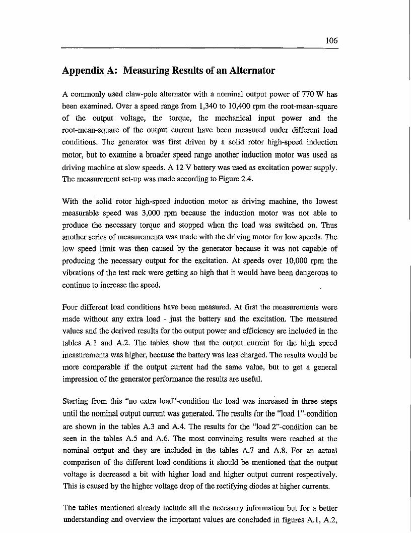
106
Appendix A: Measuring Results of an Alternator
A commonly used claw-pole alternator with a nominal output power of 770 W has
been examined. Over a speed range from 1,340 to 10,400 rpm the root-mean-square
of the output voltage, the torque, the mechanical input power and the
root-mean-square of the output current have been measured under different load
conditions. The generator was first driven by a solid rotor high-speed induction
motor, but to examine a broader speed range another induction motor was used as
driving machine at slow speeds. A 12 V battery was used as excitation power supply. The measurement set-up was made according to Figure 2.4.
With the solid rotor high-speed induction motor as driving machine, the lowest
measurable speed was 3,000 rpm because the induction motor was not able to
produce the necessary torque and stopped when the load was switched on. Thus
another series of measurements was made with the driving motor for low speeds. The
low speed limit was then caused by the generator because it was not capable of
producing the necessary output for the excitation. At speeds over 10,000 rpm the
vibrations of the test rack were getting so high that it would have been dangerous to
continue to increase the speed.
Four different load conditions have been measured. At first the measurements were
made without any extra load - just the battery and the excitation. The measured
values and the derived results for the output power and efficiency are included in the
tables A.1 and A.2. The tables show that the output current for the high speed
measurements was higher, because the battery was less charged. The results would be
more comparable if the output current had the same value, but to get a general
impression of the generator performance the results are useful.
Starting from this “no extra load”-condition the load was increased in three steps
until the nominal output current was generated. The results for the “load 1’’-condition
are shown in the tables A.3 and A.4. The results for the “load 2”-condition can be
seen in the tables A.5 and A.6. The most convincing results were reached at the
nominal output and they are included in the tables A.7 and A.8. For an actual
comparison of the different load conditions it should be mentioned that the output
voltage is decreased a bit with higher load and higher output current respectively.
This is caused by the higher voltage drop of the rectifying diodes at higher currents.
The tables mentioned already include all the necessary information but for a better
understanding and overview the important values are concluded in figures A.1, A.2,

Appendix A: Measuring Results of an Alternator 107
A.3 and A.5. Figure A.l shows the absolute value of the torque versus speed for the
different load conditions. It can be seen that the input torque shows a different
behaviour according to the load condition. At low loads the torque increases mainly
with the increase of the angular velocity but at high loads the torque decreases with
the velocity. The effect at low load is caused by the increase of losses, especially the
fan losses (see below). At high load the influence of the losses can not be seen this
straight from the torque behaviour because the high output power dominates the
behaviour and less torque is generally needed at higher speeds.
abs(7)/Nm5.0 T —no extra load
— load 1 —load 2 —loads
4.5 --
4.0"
3.5 -
3.0--
2.5--
2.0-
1.0--
1000 2000 3000 4000 5000 6000 7000 8000 9000 10000 11000
Figure A.1: Absolute value of torque versus speed for the different load conditions
Figure A.2 shows the absolute value of the mechanical input power versus speed for
the different load conditions. This figure illustrates the influence of the losses better
than the previous one because the contrary influence of the angular velocity is not
affecting the mechanical input power. It can be seen that the mechanical input power
increases for all load conditions with the increase of speed. This is caused by the
speed-depending increase of the losses.
Figure A.3 concludes the output power versus speed for the different load conditions.
It can be seen that the output power is held almost constant over a very broad speed
range and only at slow speeds some problems occur for high loads. At low loads the
generator is able to deliver the necessary output through the whole speed range but at
“load 2”-condition the generator is not able to produce the output power at speeds
under 2,000 rpm and at “load 3”-condition at speeds under 2,500 rpm. Thus only the
maximum reachable output current was measured for the “load 3”-condition under

Appendix A: Measuring Results of an Alternator 108
2,500 rpm (see Table A.8). It is impossible to get other values, because the load is
overtaken by the battery and thus it is quickly discharged. With the discharge of the
battery the voltage drops quickly and useful results can not be measured anymore.
abs(f mech)/W
2500 T
2000 --
1500 --
1000--
— no extra load— load 1 —load 2— load3
500 -
1000 2000 3000 4000 5000 6000 7000 8000 9000 10000 11000
Figure A.2: Absolute value of mechanical input power versus speed for the
different load conditions
P outAV
900 T
800 - -
700 --
600 -
500--
—no extra load — load 1 —load 2 —load 3
400 - -
300 - -
200--
1000 2000 3000 4000 5000 6000 7000 8000 9000 10000 11000
Figure A.3: Output power versus speed for the different load conditions
Figure A.4 shows the maximum output current versus speed. The current curve has
the same behaviour than expected in the theory (compare Figure 2.5). Especially
remarkable is that the nominal current can only be reached at speeds higher than

Appendix A: Measuring Results of an Alternator 109
3,000 rpm. Under this speed the maximum output current decreases rapidly with a
decrease of the speed. This behaviour explains the low maximum output power of
alternators at low speeds.
I max/A
1000 2000 3000 4000 5000 6000 7000 8000 9000 10000 11000
Figure A.4: Maximum current versus speed
Most convincing is figure A.5. It illustrates the efficiency versus speed for different
load conditions^ It can be seen that the efficiency goes down with the increase of the
speed independently of the load condition. The low efficiency for the “no extra
load"-condition is not very convincing because almost no output power is supplied.
Only the battery is slightly charged. Almost all the mechanical input power is needed
straight to cover the losses, especially at high speeds. At low speeds quite a good
efficiency is reached for all load conditions but at high speeds the efficiency is rather
poor. The maximum efficiency reached is 65 %. This is quite good, but the maximum
efficiency at nominal output is only 50 %.
The large decrease of the efficiency with an increase of the angular velocity indicates
that some of the losses are highly speed-depending. The fan losses are the most
reasonable explanation because the air resistance is highly speed-depending. To
estimate the fan losses two more measurement series were made with the driving
machine for high speeds. The first series was with the excitation turned off and for
the second series also the fan was taken away. The results are included in the tables A.9 and A. 10. From these results the fan losses can be estimated and they are
included in table Aril.

Appendix A: Measuring Results of an Alternator 110
77 in %70.0 T — no extra load
— load 1
— load 2— load 3
60.0 - -
50.0 - -
40.0 - -
30.0 - -
20.0 - -
10.0-
1000 2000 3000 4000 5000 6000 7000 8000 9000 10000 11000
Figure A.5: Efficiency versus speed for the different load conditions
Figure A.6 illustrates the measurement results and the derived fan losses. It can be
seen that the fan losses are the major part of the losses. Especially at high speeds they
rise very high up to 680 W at 8,000 rpm and at higher speeds even more. The curve
for the measurement results without excitation and fan shows the height of the rest of
the losses but it is difficult to distinguish them. They are mainly frictional losses in
the bearings and particularly the speed-depending part of the losses seems to be from
the air resistance of the clutches between the alternator and the driving machine.
abs(Pmcch)/W1200 T
— estimated fan losses —no excitation— no excitation and no fan
1000 --
800 --
600 --
400 --
200 --
4 v/rpm
Figure A.6: Absolute value of mechanical input power versus speed for the not
excited generator with and without fan and estimated fan losses

Appendix A: Measuring Results of an Alternator 111
Finally, after estimation of the fan losses the alternator efficiency without
consideration of the fan losses can be estimated. It is shown in figure A.7 for nominal
output. Its value is around 50 % and decreases slightly with the speed.
77 in %
Figure A.7: Estimated efficiency versus speed at nominal output power without
fan losses
The tables of the measuring results are following on the next pages.

Appendix A: Measuring Results of an Alternator 112
Table A. 1: Measuring results of the alternator without extra load at high speeds
v/rpm TfNm f rms/A C/rms/V P mech/W P out/W 77 in %3043 -0.736 6.8 14.10 -234.6 95.9 40.93498 -0.802 8.8 14.15 -293.8 124.5 42.44010 -0.766 8.2 14.12 -321.7 115.8 36.04507 -0.714 7.7 14.11 -337.0 108.6 32.25002 -0.722 7.6 14.11 -378.2 107.2 28.45502 -0.718 7.0 14.11 -413.7 98.8 23.95980 -0.760 6.9 14.10 -475.9 97.3 20.46519 -0.814 6.4 14.10 -555.7 90.2 16.26969 -0.854 6.2 14.11 -623.2 87.5 14.07399 -0.948 6.1 14.10 -734.6 86.0 11.78075 -1.124 5.6 14.10 -950.4 79.0 8.38836 -1.180 4.9 14.13 -1013.7 69.2 6.89177 -1.328 5.5 14.11 -1158.1 77.6 6.79691 -1.228 5.2 14.11 -1064.4 73.4 6.9
10391 -1.382 5.4 14.11 -1290.1 76.2 5.9
Table A.2: Measuring results of the alternator without extra load at low speeds
v/rpm r/Nm / rms/A C/ms/V f mech/W P out/W 77 in %1340 -0.83 2.9 14.22 -116.5 41.2 35.41500 -0.65 2.8 14.20 -102.1 39.8 38.92000 -0.42 2.5 14.19 -88.0 35.5 40.32500 -0.35 2.9 14.18 -91.6 41.1 44.93000 -0.29 2.5 14.19 -91.1 35.5 38.93500 -0.28 2.7 14.20 -102.6 38.3 37.44000 -0.30 3.3 14.18 -125.7 46.8 37.2

Appendix A: Measuring Results of an Alternator 113
Table A.3: Measuring results of the alternator for load 1 at high speeds
v/rpm 7YNm ■^rms/A t/rms/V P mech/W Pout/W 77 in %3008 -1.236 13.5 14.08 -389.3 190.1 48.83500 -1.188 14.9 14.10 -435.4 210.1 48.34012 -1.102 14.3 14.06 -463.0 201.1 43.44505 -1.012 13.5 14.07 -477.4 189.9 39.85001 -0.990 13.7 14.07 -518.5 192.8 37.25508 -0.966 13.3 14.06 -557.1 187.0 33.66016 -0.980 13.0 14.06 -617.4 182.8 29.66515 -1.008 12.7 14.07 -687.7 178.7 26.07008 -1.048 12.6 14.08 -769.1 177.4 23.17550 -1.140 12.5 14.08 -901.3 176.0 19.58010 -1.336 12.0 14.07 -1120.7 168.8 15.18824 -1.334 11.5 14.10 -1138.8 162.2 14.29166 -1.500 12.0 14.07 -1305.8 168.8 12.99681 -1.378 11.9 14.06 -1199.9 167.3 13.9
10379 -1.494 12.0 14.06 -1330.8 168.7 12.7
Table A.4: Measuring results of the alternator for load 1 at low speeds
v/rpm r/Nm ^rms/A t/rms/V P mech/W P out/W rj in %1340 -1.81 8.0 13.90 -254.0 111.2 43.81500 -1.65 10.0 14.11 -259.2 141.1 54.42000 -1.09 10.3 14.06 -228.3 144.8 63.42500 -0.85 10.3 14.07 -222.5 144.9 65.13000 -0.72 10.0 14.05 -226.2 140.5 62.13500 -0.66 10.1 14.05 -241.9 141.9 58.74000 -0.61 10.5 14.06 -255.5 147.6 57.8

Appendix A: Measuring Results of an Alternator 114
Table A.5: Measuring results of the alternator for load 2 at high speeds
v/rpm 77Nm ■^rms/A C/rms/V P mech/W P out/W Tj in %3000 -2.974 34.5 13.98 -934.3 482.3 51.64009 -2.498 35.8 14.01 -1048.7 501.6 47.84503 -2.286 35.5 14.03 -1078.0 498.1 46.25008 -2.132 35.1 13.99 -1118.0 491.0 43.95505 -2.016 35.0 13.99 -1162.1 489.7 42.16001 -1.906 34.7 13.99 -1197.7 485.5 40.56495 -1.864 34.1 14.00 -1267.7 477.4 37.76996 -1.858 34.5 14.01 -1361.2 483.3 35.57557 -1.892 34.2 14.00 -1497.4 478.8 32.08063 -2.010 33.5 13.99 -1697.1 468.7 27.68770 -1.970 33.5 14.00 -1673.1 469.0 28.09110 -2.168 33.8 13.99 -1864.1 472.9 25.49627 -1.990 33.4 13.96 -1721.8 466.3 27.1
10326 -2.046 33.5 13.96 -1817.8 467.7 25.7
Table A.6: Measuring results of the alternator for load 2 at low speeds
v/rpm r/Nm •^rms/A U rms/V P mech/W P out/W 77 in %2000 -4.10 34.0 14.03 -858.7 477.0 55.62500 -3.00 32.6 13.98 -785.4 455.7 58.03000 -2.48 32.8 13.98 -779.1 458.5 58.93500 -2.14 32.5 13.99 -784.4 454.7 58.04000 -1.93 32.8 14.00 -808.4 459.2 56.8

Appendix A: Measuring Results of an Alternator 115
Table A.7: Measuring results of the alternator for load 3 at high speeds
v/rpm 77Nm ■f rms/A t/rms/V P mech/W Pout/W 77 in %3611 -4.808 57.5 14.14 -1818.3 813.1 44.74493 -3.592 55.0 13.98 -1689.9 768.9 45.54994 -3.518 54.0 13.95 -1839.7 753.3 40.95496 -3.204 53.9 13.95 -1844.1 751.9 40.85999 -3.138 54.5 13.96 -1971.3 760.8 38.66473 -3.054 54.2 13.96 -2070.3 756.6 36.56997 -2.994 54.2 13.96 -2193.9 756.6 34.57518 -2.884 53.4 13.95 -2270.6 744.9 32.88022 -2.800 53.7 13.96 -2352.1 749.7 31.98688 -2.780 53.4 13.95 -2362.1 744.9 31.59028 -2.850 54.0 13.97 -2469.4 754.4 30.59543 -2.754 53.6 13.93 -2382.4 746.6 31.3
10249 -2.736 53.5 13.92 -2465.7 744.7 30.2
Table A.8: Measuring results of the alternator for load 3 at low speeds
v/rpm T/Nm 7 rms /A 7/ rms/V P mech/W P out/W 77 in %1340 10.01500 14.02000 34.02500 -4.52 45.5 13.11 -1183.3 596.5 50.43000 -4.71 52.5 13.86 -1479.7 727.7 49.23500 -4.49 55.4 14,01 -1645.7 776.2 47.24000 -3.80 55.0 13.95 -1591.7 767.3 48.2
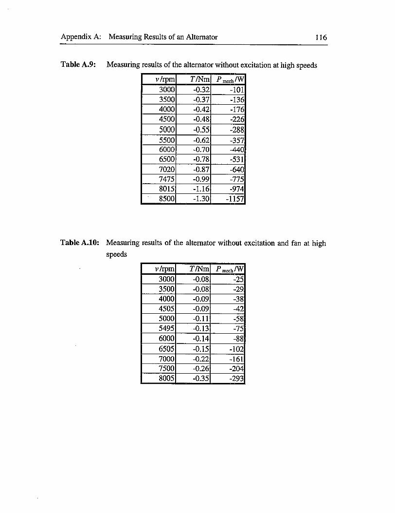
Appendix A: Measuring Results of an Alternator 116
Table A.9:
Table A.10:
Measuring results of the alternator without excitation at high speeds
v/rpm 77Nm P mech /W3000 -0.32 -1013500 -0.37 -1364000 -0.42 -1764500 -0.48 -2265000 -0.55 -2885500 -0.62 -3576000 -0.70 -4406500 -0.78 -5317020 -0.87 -6407475 -0.99 -7758015 -1.16 -9748500 -1.30 -1157
Measuring results of the alternator without excitation and fan at high
speeds
v/rpm T/Nm -Pmech/W3000 -0.08 -253500 -0.08 -294000 -0.09 -384505 -0.09 -425000 -0.11 -585495 -0.13 -756000 -0.14
OO
oot
6505 -0.15 -1027000 -0.22 -1617500 -0.26 -2048005 -0.35 -293

Appendix A: Measuring Results of an Alternator 117
Table A.ll: Derived fan losses from the alternator measurements
v/rpm P mech/W3000 753500 1054000 1404500 1855000 2305500 2806000 3506500 4307000 4807500 5708000 680
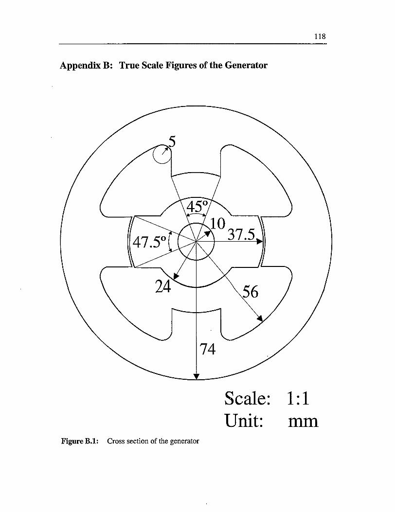
118
Appendix B: True Scale Figures of the Generator
Scale:mm
Figure B.l: Cross section of the generator

Appendix B: True Scale Figures of the Generator 119
Scale: 1:1 Unit: mm
Figure B.2: Longitudinal cross section of the generator

120
Appendix C: Conclusion of Characteristic and Dimension
Values
Nominal voltage
Nominal current
Nominal output power
Minimum speed Maximum speed
Number of stator poles
Number of rotor poles
Shaft radius
Minor rotor radius
Rotor radius
Radius of stator slot bottom
Stator outside radius
Stack length
Overall length
Air gap length
Stator pole arc
Rotor pole arc
Radius of comer at stator slot bottom
Lamination stacking factor
Layer thickness of the lamination stacking
Number of parallel path per phase
Number of turns per pole
Slot fill factor
Thickness of insulation layer
Slot area
Copper area
Direct-current phase resistance (20 °C)
Direct-current phase resistance (90 °C)
Iron weight
Copper weight
Total weight
Moment of inertia
Z7n=14V
7n= 107 A
PN= 1.5 kW
Vmin= 1,200 rpm
Vmax= 12,000 rpm
Ns = 4
Nr= 2
RSh = 10 mm
Ro = 24 mm
R\ = 37.5 mm
i?2 = 56 mm
i?3 = 74 mm
L$tk = 75 nun
Le= 133.5 mm
<5= 0.3 mm
A = 45°
A =47.5° r-5 mm
/stk = 0.97
rstk= 0.5 mm
Npath = 1
Nv = 12
Sfin= 0.576
d = 0.2 mm Asiot= 786 mm2
Acu = 226 mm2
PphDC(20) = 6.3 m£2
PphDC(9o> =8.0 mQ WFe= 6.7 kg
Wcu = 2.4 kg
Wtot= 9.1 kg / = 7.94*10"4 kgm2
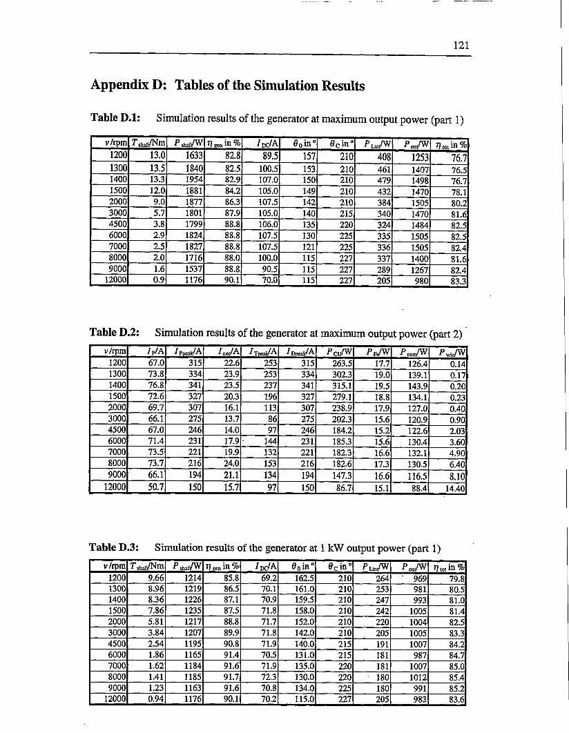
121
Appendix D: Tables of the Simulation Results
Table D.l: Simulation results of the generator at maximum output power (part 1)
v/rpm T shaii/Nm P shaf/W T] gen HI % I dc/A 6oin° 0cin° fiVW P ou,/W 77 tot in %1200 13.0 1633 82.8 89.5 157 210 408 1253 76.71300 13.5 1840 82.5 100.5 153 210 461 1407 76.51400 13.3 1954 82.9 107.0 150 210 479 1498 76.71500 12.0 1881 84.2 105.0 149 210 432 1470 78.12000 9.0 1877 86.3 107.5 142 210 384 1505 80.23000 5.7 1801 87.9 105.0 140 215 340 1470 81.64500 3.8 1799 88.8 106.0 135 220 324 1484 82.56000 2.9 1824 88.8 107.5 130 225 335 1505 82.57000 2.5 1827 88.8 107.5 121 225 336 1505 82.48000 2.0 1716 88.0 100.0 115 227 337 1400 81.69000 1.6 1537 88.8 90.5 115 227 289 1267 82.4
12000 0.9 1176 90.1 70.0 115 227 205 980 83.3
Table D.2: Simulation results of the generator at maximum output power (part 2)
v/rpm / p/A /pocak/A IcJA /rocak/A I Doeafc/A fcu/W PeVW P cott/W Pwit/W1200 67.0 315 22.6 253 315 263.5 17.7 126.4 0.141300 73.8 334 23.9 253 334 302.3 19.0 139.1 0.171400 76.8 341 23.5 237 341 315.1 19.5 143.9 0.201500 72.6 327 20.3 196 327 279.1 18.8 134.1 0.232000 69.7 307 16.1 113 307 238.9 17.9 127.0 0.403000 66.1 275 13.7 86 275 202.3 15.6 120.9 0.904500 67.0 246 14.0 97 246 184.2 15.2 122.6 2.036000 71.4 231 17.9 144 231 185.3 15.6 130.4 3.607000 73.5 221 19.9 132 221 182.3 16.6 132.1 4.908000 73.7 216 24.0 153 216 182.6 17.3 130.5 6.409000 66.1 194 21.1 134 194 147.3 16.6 116.5 8.10
12000 50.7 150 15.7 97 150 86.7 15.1 88.4 14.40
Table D.3: Simulation results of the generator at 1 kW output power (part 1)
v/rpm T shafi/Nm P shaf/W 7? sen in % /dc/A 0o in" 0c in" P u=t/W Pout/W 7? tot in %1200 9.66 1214 85.8 69.2 162.5 210 264 " 969 79.81300 8.96 1219 86.5 70.1 161.0 210 253 981 80.51400 8.36 1226 87.1 70.9 159.5 210 247 993 81.01500 7.86 1235 87.5 71.8 158.0 210 242 1005 81.42000 5.81 1217 88.8 71.7 152.0 210 220 1004 82.53000 3.84 1207 89.9 71.8 142.0 210 205 1005 83.34500 2.54 1195 90.8 71.9 140.0 215 191 1007 84.26000 1.86 1165 91.4 70.5 131.0 215 181 987 84.77000 1.62 1184 91.6 71.9 135.0 220
OO 1007 85.0
8000 1.41 1185 91.7 72.3 130.0 220 180 1012 85.49000 1.23 1163 91.6 70.8 134.0 225 180 991 85.2
12000 0.94 1176 90.1 70.2 115.0 227 205 983 83.6

Appendix D: Tables of the Simulation Results 122
Table D.4: Simulation results of the generator at 1 kW output power (part 2)
v/rpm /p/A I Pocak/A / cx(/A ■Itdoi/A 1 Doeak/A PcuAV PrAV f con/W /’winAV1200 49.8 262 ' 15.4 178 262 158.1 14.2 91.1 0.141300 49.0 261 14.1 153 261 150.1 14.0 89.1 0.171400 48.5 259 13.2 133 259 144.5 13.9 87.9 0.201500 48.3 257 12.5 117 257 140.8 13.8 87.4 0.232000 46.3 243 10.5 61 243 122.3 13.4 83.7 0.403000 45.8 220 10.0 32 220 108.0 13.5 82.8 0.904500 44.9 195 9.0 31 195 95.1 12.6 81.7 2.036000 44.5 174 9.3 28 174 83.4 13.2 80.6 3.607000 44.7 167 8.8 34 167 81.9 12.7 81.4 4.908000 45.2 159 9.0 32 159 78.4 13.1 82.0 6.409000 45.2 154 9.9 75 154 77.1 12.7 82.0 8.10
12000 50.7 150 15.7 97 150 86.7 15.1 88.4 14.40
Table D.5: Simulation results of the generator at 0.5 lcW output power (part 1)
v/rpm rshafl/Nm Pshaf/W V gen in % /dc/A 0O in0 0c in” P Lto/W Pou/W 7? tot in %1200 4.87 612 90.0 37.0 172.5 210 108 518 84.61300 4.24 577 90.5 34.7 171.5 210 98 486 84.21400 4.07 596 90.6 35.9 170.0 210 100 503 84.31500 3.85 604 90.8 36.4 169.0 210 100 510 84.42000 2.77 579 91.4 35.3 165.0 210 92 494 85.43000 1.91 600 92.0 36.5 157.0 210 92 511 85.24500 1.25 590 92.6 36.2 149.0 210 86 507 85.96000 0.92 578 92.9 35.5 143.0 210 82 497 86.07000 0.80 586 92.9 36.1 139.0 210 83 505 86.28000 0.70 589 92.9 36.3 145.0 215 83 508 86.39000 0.62 584 92.8 35.9 142.0 215 83 503 86.1
12000 0.47 584 92.1 35.7 143.0 220 86 500 85.6
Table D.6: Simulation results of the generator at 0.5 kW output power (part 2)
v/rpm / p/A f Pocak/A Axe/A ■^Tocak/A I Dpeal/A Pcu/W PreAV Pcon/W PwinAV
1200 26.3 176 7.8 84 176 52.0 9.2 46.3 0.141300 24.7 170 7.4 65 170 45.4 9.0 43.3 0.171400 25.2 173 7.3 5.7 173 46.5 9.1 44.2 0.201500 25.3 174 7.1 50 174 46.4 9.1 44.5 0.232000 24.0 165 6.4 32 165 40.7 8.9 42.3 0.403000 24.4 153 6.1 27 153 38.2 9.2 43.2 0.904500 23.7 133 5.6 22 133 32.2 9.5 42.2 2.036000 23.0 119 5.2 19 119 27.9 9.7 41.1 3.607000 23.2 113 5.2 18 113 26.9 10.0 41.5 4.908000 22.9 109 4.7 20 109 26.2 9.4 41.3 6.409000 22.6 103 4.6 19 103 24.5 9.6 40.8 8.10
12000 22.3 93 4.5 22 93 22.2 9.5 40.4 14.40
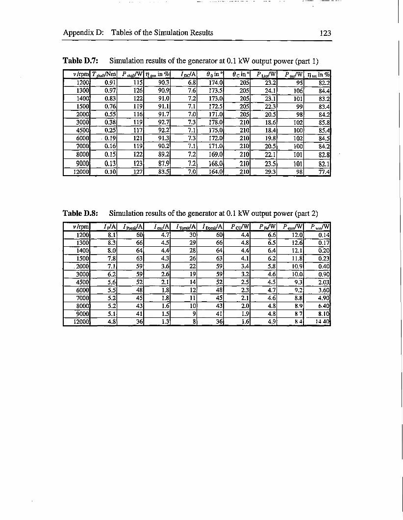
Appendix D: Tables of the Simulation Results 123
Table D.7: Simulation results of the generator at 0.1 kW output power (part 1)
v/rpm T sbaf/Nm P shaf/W 1} gen in % I dc/A 0oin° 9cin° fuo/W P ou/W T] lot in %1200 0.91 115 90.3 6.8 174.0 205 23.2 95 82.21300 0.97 126 90.9 7.6 173.5 205 24.1 106 84.41400 0.83 122 91.0 7.2 173.0 205 23.1 101 83.21500 0.76 119 91.1 7.1 172.5 205 22.3 99 83.42000 0.55 116 91.7 7.0 171.0 205 20.5 98 84.23000 0.38 119 92.7 7.3 178.0 210 18.6 102 85.84500 0.25 117 92.2 7.1 175.0 210 18.4 100 85.46000 0.19 121 91.3 7.3 172.0 210 19.8 102 84.57000 0.16 119 90.2 7.1 171.0 210 20.5 100 84.28000 0.15 122 89.2 7.2 169.0 210 22.1 101 82.8
9000 0.13 123 87.9 7.2 168.0 210 23.5 101 82.112000 0.10 127 83.5 7.0 164.0 210 29.3 98 77.4
Table D.8: Simulation results of the generator at 0.1 kW output power (part 2)
v/rpm / p/A I Plicak/A WA / TDcal/A I Doeak/A PcuAV Pr/W Pcom/W Pwu/W
1200 8.1 60 4.7 30 60 4.4 6.6 12.0 0.141300 8.3 66 4.5 29 66 4.8 6.5 12.6 0.171400 8.0 64 4.4 28 64 4.4 6.4 12.1 0.201500 7.8 63 4.3 26 63 4.1 6.2 11.8 0.23
.2000 7.1 59 3.6 22 59 3.4 5.8 10.9 0.403000 6.2 59 2.6 19 59 3.2 4.6 10.0 0.904500 5.6 52 2.1 14 52 2.5 4.5 9.3 2.036000 5.5 48 1.8 12 48 2.3 4.7 9.2 3.607000 5.2 45 1.8 11 45 2.1 4.6 8.8 4.908000 5.2 43 1.6 10 43 2.0 4.8 8.9 6409000 5.1 41 1.5 9 41 1.9 4.8 87 8.10
12000 4.8 36 1.3 8 36 1.6 4.9 84 14 40