LARGE-SCALE INTEGRATION OF HETEROGENEOUS SIMULATIONS

By

HIMANSHU NEEMA

Dissertation

Submitted to the Faculty of the

Graduate School of Vanderbilt University

in partial fulfillment of the requirements

for the degree of

DOCTOR OF PHILOSOPHY

in

Computer Science

January 31, 2018

Nashville, Tennessee

Approved:

Gabor Karsai, Chair, Ph.D.

Janos Sztipanovits, Ph.D.

Gautam Biswas, Ph.D.

Jules White, Ph.D.

Bharat Bhuva, Ph.D.

ii

Copyright © 2018 by Himanshu Neema All Rights Reserved

iii

DEDICATION

I dedicate this dissertation to my late father, Suresh Chandra Neema, my mother, Gita Neema, my beloved and supportive wife, Reena Neema, and my amazing and loving children, Sanya and Vivaan, for their love and wisdom, and their incessant belief in me,

And my brother, Ritesh Neema, and sister-in-law, Raina Neema, for always being there for me,

And the rest of my loving and supportive family including Kavish Neema, Supriya Neema, Vaibhav Doshi, Purvashi Doshi, Sandeep Neema, Payal Neema, Jagdish Chandra Neema, and Natwarlal Neema.

This work would not have been possible without your encouragement, love, dedication, and support. I am and will forever be grateful for all you have done for me.

iv

ACKNOWLEDGEMENTS

This research in part was sponsored by the US Air Force Office of Scientific Research (AFOSR), under contract number FA9550-06-1-0267, US Air Force Research Lab Information Directorate (AFRL/RI), under contract number FA8750-11-2-0078, US Defense Advanced Research Projects Agency (DARPA), under contract number HR0011-12-C-0008, and US Air Force Research Lab, under contract FA8750-14-2-0180. The views and conclusions contained herein are those of the author and should not be interpreted as necessarily representing the official policies or endorsements, either expressed or implied, of AFOSR, AFRL/RI, DARPA, AFRL, or the US Government. I would like to thank the above funding agencies for supporting this research.

I would like to acknowledge the superior guidance of my advisor and the chair of my dissertation committee, Dr. Gabor Karsai. He has always provided me with his highly sincere and pertinent advice throughout my research. I have found him to exceptionally thorough in the knowledge and understanding of core concepts of all his research areas. Despite his busy schedule, he has always provided timely feedback on all my queries. He has also always provided precise answers for all of my research questions. Thank you, Professor, for all your help and support you have given me.

I am also grateful to the members of my dissertation committee, Dr. Janos Sztipanovits, Dr. Gautam Biswas, Dr. Jules White, and Dr. Bharat Bhuva for sharing their highly insightful guidance. They all have tremendous experience in this research area and I have greatly benefitted from having them on my dissertation committee.

I would also like to take this opportunity to acknowledge the Institute for Software Integrated Systems at Vanderbilt University for supporting my research through last many years and its Director, Dr. Janos Sztipanovits, for his highly visionary insights. Thank you.

v

TABLE OF CONTENTS

DEDICATION .................................................................................................................................... iii

ACKNOWLEDGEMENTS ................................................................................................................... iv

TABLE OF CONTENTS........................................................................................................................ v

LIST OF TABLES ................................................................................................................................. x

LIST OF FIGURES .............................................................................................................................. xi

LIST OF ABBREVIATIONS ............................................................................................................... xiii

CHAPTER 1. INTRODUCTION ........................................................................................................... 1

1.1 Overview ............................................................................................................................... 1

1.2 Approach ............................................................................................................................... 2

1.3 Scope ..................................................................................................................................... 3

1.4 Assumptions .......................................................................................................................... 3

1.5 Dissertation Organization ..................................................................................................... 4

CHAPTER 2. BACKGROUND ............................................................................................................. 5

2.1 Sources of Heterogeneity in Large SoS ................................................................................. 5

2.1.1 Systems .......................................................................................................................... 5

2.1.2 Models ........................................................................................................................... 5

2.1.3 Physical Domains ........................................................................................................... 6

2.1.4 Models of Computation ................................................................................................. 7

2.1.5 Simulators ...................................................................................................................... 7

2.1.6 Modeling Languages ...................................................................................................... 8

2.1.7 Time Scales and Resolutions .......................................................................................... 8

2.1.8 Simulation Techniques ................................................................................................... 9

2.1.9 Time Synchronization Methods ................................................................................... 10

2.1.10 Execution Environments ............................................................................................ 11

2.1.11 Communication Patterns ........................................................................................... 11

2.1.12 Summary of Heterogeneity Impact on SoS simulations ............................................ 12

2.2. Core requirements for distributed co-simulation of real-world system-of-systems ........ 12

2.2.1 Fundamental Requirements ........................................................................................ 12

2.2.2 Modeling, Simulation, and Experimentation Requirements ....................................... 16

2.2.3 Usability Requirements ................................................................................................ 18

2.2.4 Cyber Requirements .................................................................................................... 19

vi

2.2.5 Evolutionary Requirements (Flexibility, Adaptability, Extensibility)............................ 20

2.2.6 Summary of Real-World Distributed Co-Simulation Requirements ............................ 20

2.3. Co-simulation standards and approaches ......................................................................... 20

2.3.1 Standards for Distributed Simulations ......................................................................... 20

2.3.2 Frameworks and Methods for Co-Simulation .............................................................. 26

2.3.3 Summary ...................................................................................................................... 28

2.4. Ontologies for model composition .................................................................................... 28

2.4.1 Introduction ................................................................................................................. 28

2.4.2 Background on ontologies ........................................................................................... 30

2.4.3 Related Work ............................................................................................................... 31

2.4.4 Summary of current ontological approaches in simulations ....................................... 33

CHAPTER 3. RESEARCH PROBLEMS AND HYPOTHESIS ................................................................. 34

3.1 Research Problems ............................................................................................................. 34

3.2 Research Hypothesis ........................................................................................................... 34

CHAPTER 4. MODEL-BASED INTEGRATION FOR DISTRIBUTED SIMULATION EXPERIMENTS ....... 35

4.1 Introduction ........................................................................................................................ 35

4.2 Architectural Overview ....................................................................................................... 36

4.2.1 Model Integration Platform ......................................................................................... 37

4.2.2 Simulation Integration Platform .................................................................................. 39

4.2.3 Execution Integration Platform .................................................................................... 40

4.3 Model Integration Environment ......................................................................................... 40

4.3.1 Integration Overview ................................................................................................... 42

4.3.2 Integration Modeling Language ................................................................................... 43

4.3.3 Integration Modeling ................................................................................................... 46

4.3.4 Federation Execution Semantics .................................................................................. 47

4.4 Simulation Engine Integration ............................................................................................ 48

4.4.1 OMNeT++: Communication Network Simulation ........................................................ 48

4.4.2 Matlab/Simulink: Dynamics and Control Simulation ................................................... 49

4.4.3 CPN Tools: Parallel Processes and Workflows Simulation ........................................... 50

4.5 Deployment Modeling and Execution ................................................................................ 51

4.5.1 Deployment Modeling ................................................................................................. 51

4.5.2 Federation Manager .................................................................................................... 53

4.6 Hardware In the Loop (HIL) Simulation .............................................................................. 55

4.6.1 Fundamental Issues with HIL ....................................................................................... 56

4.6.2 Platform Architecture .................................................................................................. 58

4.6.3 Simulation Example...................................................................................................... 59

4.7 Large-Scale Simulation Integration: Case Study ................................................................. 60

vii

4.8 Levels of Users of the Integration Framework ................................................................... 62

4.9 Summary ............................................................................................................................. 62

CHAPTER 5. MAPPING METHODS FOR LEGACY COMPONENT INTEGRATION ............................. 63

5.1 Introduction ........................................................................................................................ 63

5.2 Related Work ...................................................................................................................... 64

5.3 Mapper Federate Overview ................................................................................................ 64

5.4 Mapping Types .................................................................................................................... 65

5.5 Mapping Code ..................................................................................................................... 68

5.6 Performance Considerations .............................................................................................. 68

5.7 Summary ............................................................................................................................. 69

CHAPTER 6. REUSABLE COMPONENT FOR CYBER COMMUNICATION NETWORK SIMULATION . 70

6.1 Introduction ........................................................................................................................ 70

6.2 Integrating OMNeT++ Scheduler ........................................................................................ 71

6.3 Creating a Reusable Network Simulation Federate ............................................................ 72

6.4 Mappings for NetworkPacket Encapsulation and Decapsulation ...................................... 73

6.5 Performance Considerations .............................................................................................. 73

6.6 Example Use-Cases ............................................................................................................. 74

6.6.1 Multiple Network Simulation ....................................................................................... 74

6.6.2 Mixed Wired and Wireless Simulation ........................................................................ 74

6.7 Summary ............................................................................................................................. 75

CHAPTER 7. PARTITIONING DYNAMIC MODELS FOR EFFICIENT CO-SIMULATION ...................... 76

7.1 Introduction ........................................................................................................................ 76

7.1.1 Approach ...................................................................................................................... 76

7.1.2 Chapter Organization ................................................................................................... 77

7.2 Research Paper on Integrating FMI Co-Simulations ........................................................... 78

7.2.1 Introduction ................................................................................................................. 78

7.2.2 C2 Wind Tunnel ............................................................................................................ 80

7.2.3 FMI for Co-Simulation .................................................................................................. 81

7.2.4 Model-Based Integration ............................................................................................. 81

7.2.5 Case Study .................................................................................................................... 84

7.2.6 Conclusions .................................................................................................................. 90

7.2.7 Acknowledgements ...................................................................................................... 90

7.3 Software implementation ................................................................................................... 91

7.4 Guidelines for systematic partitioning and tuning of models ............................................ 92

viii

7.5 Summary ............................................................................................................................. 92

CHAPTER 8. MODULAR CYBER-ATTACK LIBRARY FOR CYBER RESILIENCE EVALUATION ............. 93

8.1 Introduction ........................................................................................................................ 93

8.2 Framework Extensions for Implementing the Cyber-Attack Library .................................. 94

8.3 Attacks Implemented in the Cyber-Attack Library ............................................................. 95

8.4 Evaluating SoS Against Cyber-Attacks ................................................................................ 96

8.5 Summary ............................................................................................................................. 97

CHAPTER 9. COURSES-OF-ACTION EVALUATION FOR SCENARIO-BASED EXPERIMENTATION .... 98

9.1 Introduction ........................................................................................................................ 98

9.2 COA Modeling Language ................................................................................................... 100

9.3 COA Integration with Cyber-Attack Library ...................................................................... 101

9.4 COA Orchestration Engine ................................................................................................ 102

9.5 Cyber Gaming with COA Groups ....................................................................................... 103

9.6 Experiment Controller ...................................................................................................... 104

9.7 Summary ........................................................................................................................... 105

10. ONTOLOGY-BASED MODEL COMPOSITION .......................................................................... 106

10.1 Introduction .................................................................................................................... 106

10.2 Ontology Modeling Language ......................................................................................... 107

10.3 Creating Ontologies and Mapping Rules ........................................................................ 110

10.3.1 Ontology Modeling .................................................................................................. 110

10.3.2 Ontological System Modeling .................................................................................. 112

10.3.3 Modeling Ontological Mapping Rules ...................................................................... 113

10.4 Networked Sensor Controller Case Study ...................................................................... 114

10.5 Summary ......................................................................................................................... 119

11. RESULTS, CONCLUSIONS, FUTURE WORK, AND BROADER IMPACT ..................................... 120

11.1 Results ............................................................................................................................. 120

11.1.1 Challenge Problems Addressed ............................................................................... 120

11.1.2 Evaluation of Research Hypothesis with Research Results ..................................... 122

11.2 Conclusions ..................................................................................................................... 123

11.3 Future Work .................................................................................................................... 123

11.4 Broader Impact ............................................................................................................... 125

11.4.1 Simulation-based studies ......................................................................................... 125

ix

11.4.2 Research communities for web-based collaborative modeling and simulation ..... 125

11.4.3 Transition to external lab as open-source tools ...................................................... 125

11.4.4 Web-based platform for CPS security and resilience researchers .......................... 126

APPENDIX A: METAMODEL FOR THE MAPPER FEDERATE AND MAPPING SPECIFICATIONS ..... 127

APPENDIX B: SAMPLE CODE LISTINGS FOR THE CYBER-ATTACK LIBRARY .................................. 128

APPENDIX C: SIMULATORS INTERFACED IN THE INTEGRATION FRAMEWORK .......................... 130

APPENDIX D: LEVELS OF USERS OF THE INTEGRATION FRAMEWORK ....................................... 132

APPENDIX E: CYBER ATTACKS IMPLEMENTED IN THE CYBER-ATTACK LIBRARY ........................ 133

REFERENCES ................................................................................................................................ 136

x

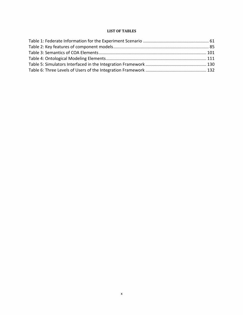
LIST OF TABLES

Table 1: Federate Information for the Experiment Scenario ....................................................... 61

Table 2: Key features of component models ................................................................................ 85

Table 3: Semantics of COA Elements .......................................................................................... 101

Table 4: Ontological Modeling Elements .................................................................................... 111

Table 5: Simulators Interfaced in the Integration Framework ................................................... 130

Table 6: Three Levels of Users of the Integration Framework ................................................... 132

xi

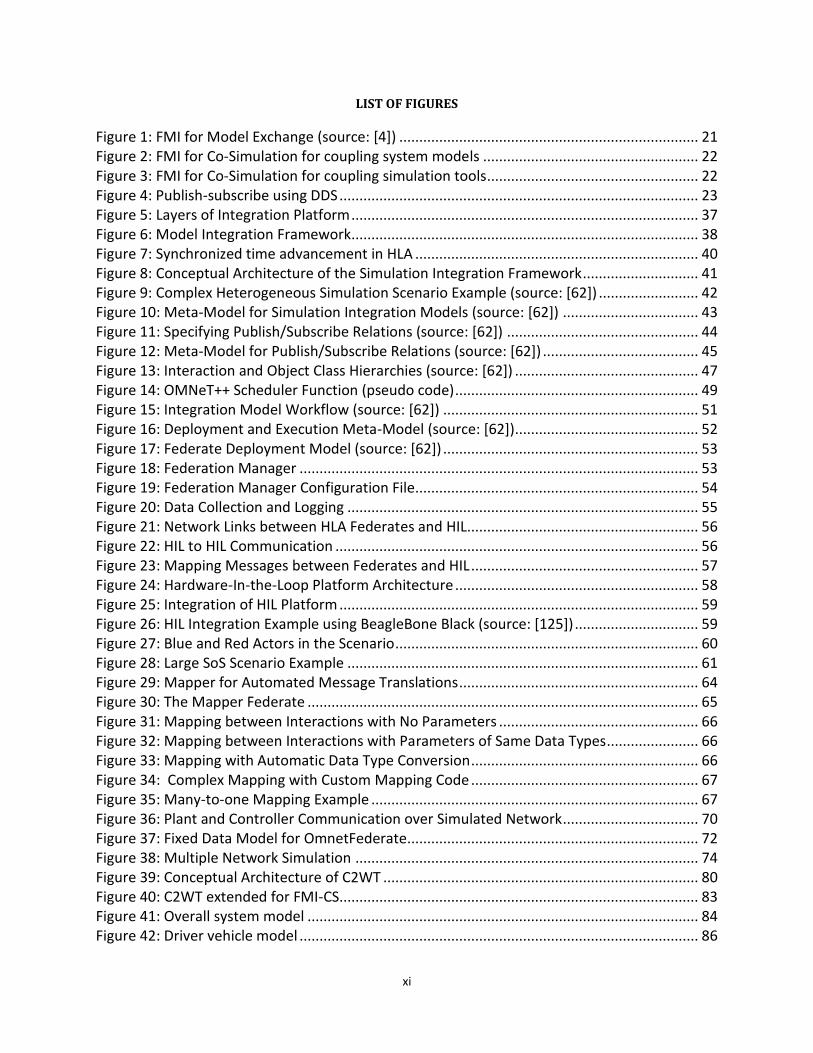
LIST OF FIGURES

Figure 1: FMI for Model Exchange (source: [4]) ........................................................................... 21

Figure 2: FMI for Co-Simulation for coupling system models ...................................................... 22

Figure 3: FMI for Co-Simulation for coupling simulation tools ..................................................... 22

Figure 4: Publish-subscribe using DDS .......................................................................................... 23

Figure 5: Layers of Integration Platform ....................................................................................... 37

Figure 6: Model Integration Framework....................................................................................... 38

Figure 7: Synchronized time advancement in HLA ....................................................................... 40

Figure 8: Conceptual Architecture of the Simulation Integration Framework ............................. 41

Figure 9: Complex Heterogeneous Simulation Scenario Example (source: [62]) ......................... 42

Figure 10: Meta-Model for Simulation Integration Models (source: [62]) .................................. 43

Figure 11: Specifying Publish/Subscribe Relations (source: [62]) ................................................ 44

Figure 12: Meta-Model for Publish/Subscribe Relations (source: [62]) ....................................... 45

Figure 13: Interaction and Object Class Hierarchies (source: [62]) .............................................. 47

Figure 14: OMNeT++ Scheduler Function (pseudo code) ............................................................. 49

Figure 15: Integration Model Workflow (source: [62]) ................................................................ 51

Figure 16: Deployment and Execution Meta-Model (source: [62]) .............................................. 52

Figure 17: Federate Deployment Model (source: [62]) ................................................................ 53

Figure 18: Federation Manager .................................................................................................... 53

Figure 19: Federation Manager Configuration File....................................................................... 54

Figure 20: Data Collection and Logging ........................................................................................ 55

Figure 21: Network Links between HLA Federates and HIL .......................................................... 56

Figure 22: HIL to HIL Communication ........................................................................................... 56

Figure 23: Mapping Messages between Federates and HIL ......................................................... 57

Figure 24: Hardware-In-the-Loop Platform Architecture ............................................................. 58

Figure 25: Integration of HIL Platform .......................................................................................... 59

Figure 26: HIL Integration Example using BeagleBone Black (source: [125]) ............................... 59

Figure 27: Blue and Red Actors in the Scenario ............................................................................ 60

Figure 28: Large SoS Scenario Example ........................................................................................ 61

Figure 29: Mapper for Automated Message Translations ............................................................ 64

Figure 30: The Mapper Federate .................................................................................................. 65

Figure 31: Mapping between Interactions with No Parameters .................................................. 66

Figure 32: Mapping between Interactions with Parameters of Same Data Types ....................... 66

Figure 33: Mapping with Automatic Data Type Conversion ......................................................... 66

Figure 34: Complex Mapping with Custom Mapping Code ......................................................... 67

Figure 35: Many-to-one Mapping Example .................................................................................. 67

Figure 36: Plant and Controller Communication over Simulated Network .................................. 70

Figure 37: Fixed Data Model for OmnetFederate......................................................................... 72

Figure 38: Multiple Network Simulation ...................................................................................... 74

Figure 39: Conceptual Architecture of C2WT ............................................................................... 80

Figure 40: C2WT extended for FMI-CS .......................................................................................... 83

Figure 41: Overall system model .................................................................................................. 84

Figure 42: Driver vehicle model .................................................................................................... 86

xii

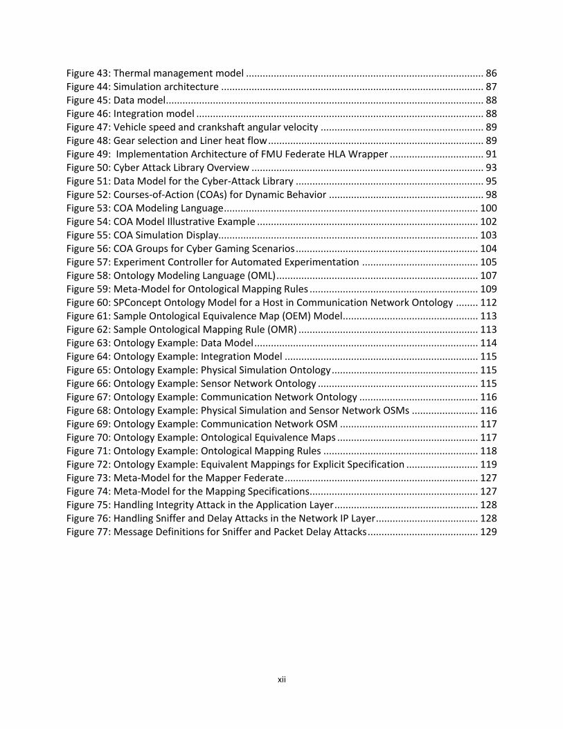
Figure 43: Thermal management model ...................................................................................... 86

Figure 44: Simulation architecture ............................................................................................... 87

Figure 45: Data model ................................................................................................................... 88

Figure 46: Integration model ........................................................................................................ 88

Figure 47: Vehicle speed and crankshaft angular velocity ........................................................... 89

Figure 48: Gear selection and Liner heat flow .............................................................................. 89

Figure 49: Implementation Architecture of FMU Federate HLA Wrapper .................................. 91

Figure 50: Cyber Attack Library Overview .................................................................................... 93

Figure 51: Data Model for the Cyber-Attack Library .................................................................... 95

Figure 52: Courses-of-Action (COAs) for Dynamic Behavior ........................................................ 98

Figure 53: COA Modeling Language ............................................................................................ 100

Figure 54: COA Model Illustrative Example ................................................................................ 102

Figure 55: COA Simulation Display.............................................................................................. 103

Figure 56: COA Groups for Cyber Gaming Scenarios .................................................................. 104

Figure 57: Experiment Controller for Automated Experimentation .......................................... 105

Figure 58: Ontology Modeling Language (OML) ......................................................................... 107

Figure 59: Meta-Model for Ontological Mapping Rules ............................................................. 109

Figure 60: SPConcept Ontology Model for a Host in Communication Network Ontology ........ 112

Figure 61: Sample Ontological Equivalence Map (OEM) Model................................................. 113

Figure 62: Sample Ontological Mapping Rule (OMR) ................................................................. 113

Figure 63: Ontology Example: Data Model ................................................................................. 114

Figure 64: Ontology Example: Integration Model ...................................................................... 115

Figure 65: Ontology Example: Physical Simulation Ontology ..................................................... 115

Figure 66: Ontology Example: Sensor Network Ontology .......................................................... 115

Figure 67: Ontology Example: Communication Network Ontology ........................................... 116

Figure 68: Ontology Example: Physical Simulation and Sensor Network OSMs ........................ 116

Figure 69: Ontology Example: Communication Network OSM .................................................. 117

Figure 70: Ontology Example: Ontological Equivalence Maps ................................................... 117

Figure 71: Ontology Example: Ontological Mapping Rules ........................................................ 118

Figure 72: Ontology Example: Equivalent Mappings for Explicit Specification .......................... 119

Figure 73: Meta-Model for the Mapper Federate ...................................................................... 127

Figure 74: Meta-Model for the Mapping Specifications............................................................. 127

Figure 75: Handling Integrity Attack in the Application Layer .................................................... 128

Figure 76: Handling Sniffer and Delay Attacks in the Network IP Layer ..................................... 128

Figure 77: Message Definitions for Sniffer and Packet Delay Attacks ........................................ 129

xiii

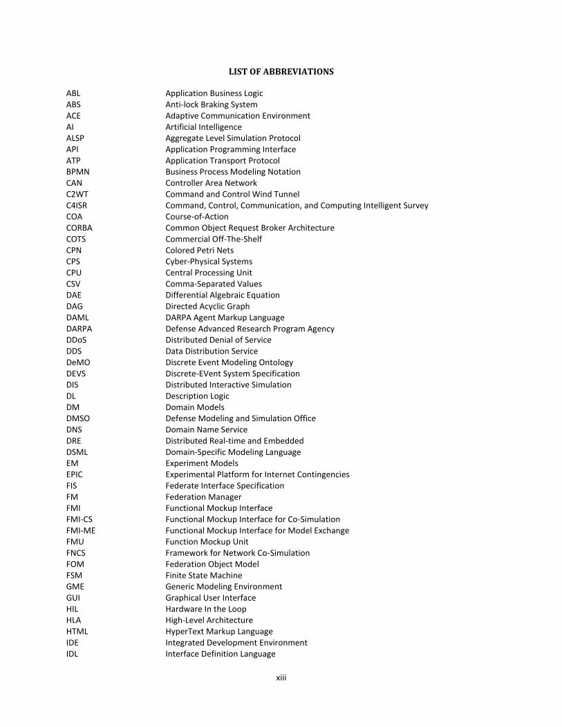
LIST OF ABBREVIATIONS

ABL Application Business Logic ABS Anti-lock Braking System ACE Adaptive Communication Environment AI Artificial Intelligence ALSP Aggregate Level Simulation Protocol API Application Programming Interface ATP Application Transport Protocol BPMN Business Process Modeling Notation CAN Controller Area Network C2WT Command and Control Wind Tunnel C4ISR Command, Control, Communication, and Computing Intelligent Survey COA Course-of-Action CORBA Common Object Request Broker Architecture COTS Commercial Off-The-Shelf CPN Colored Petri Nets CPS Cyber-Physical Systems CPU Central Processing Unit CSV Comma-Separated Values DAE Differential Algebraic Equation DAG Directed Acyclic Graph DAML DARPA Agent Markup Language DARPA Defense Advanced Research Program Agency DDoS Distributed Denial of Service DDS Data Distribution Service DeMO Discrete Event Modeling Ontology DEVS Discrete-EVent System Specification DIS Distributed Interactive Simulation DL Description Logic DM Domain Models DMSO Defense Modeling and Simulation Office DNS Domain Name Service DRE Distributed Real-time and Embedded DSML Domain-Specific Modeling Language EM Experiment Models EPIC Experimental Platform for Internet Contingencies FIS Federate Interface Specification FM Federation Manager FMI Functional Mockup Interface FMI-CS Functional Mockup Interface for Co-Simulation FMI-ME Functional Mockup Interface for Model Exchange FMU Function Mockup Unit FNCS Framework for Network Co-Simulation FOM Federation Object Model FSM Finite State Machine GME Generic Modeling Environment GUI Graphical User Interface HIL Hardware In the Loop HLA High-Level Architecture HTML HyperText Markup Language IDE Integrated Development Environment IDL Interface Definition Language

xiv

IEC International Electrotechnical Commission IED Improvised Explosive Device IP Internet Protocol JSON Java Script Object Notation KML Keyhole Markup Language LAN Local Area Network LCL Liquid Cooling Library MANET Mobile Ad-hoc NETwork MIC Model-Integrated Computing MIL Model Integration Language MoC Model of Computation NTP Network Time Protocol OEM Ontological Equivalence Map OIL Ontology Interface Layer OMG Object Management Group OML Ontology Modeling Language OMR Ontological Mapping Rule OMT Object Model Template OSM Ontological System Model OWL Web Ontology Language P2P Point to Point PDU Protocol Data Unit PIMODES Process Interaction Modeling Ontology for Discrete Event Simulations QoS Quality of Service RDF Resource Description Framework RMI Remote Method Invocation RO Receive Order RPR-FOM Real-time Platform-level Reference Federation Object Model RTI Run-Time Infrastructure RuleML Rule Markup Language SCADA Supervisory Control And Data Acquisition SDO Stateful Distributed Object SEM ScEnario Models SIGINT SIGnal INTelligence SIL System In the Loop SIMNET Simulation Network SM System Models SOA Service-Oriented Architecture SOAP Simple Object Access Protocol SOM Simulation Object Model SoS System of Systems SURE SecURE and REslient Cyber-Physical Systems SWRL Semantic Web Rule Language TAG Time Advance Grant TAR Time Advance Request TCP Transmission Control Protocol TENA Test and training ENabling Architecture TM Test Models TRaCI Traffic Control Interface TSO Time-Stamped Order UAV Unmanned Aerial Vehicle UCEF Universal Cyber-Physical Systems Environment for Federation UDP User Datagram Protocol

xv

UML Unified Modeling Language VDL Vehicle Dynamics Library VM Virtual Machine VTM Vehicle Thermal Management W3C World Wide Web Consortium WebGME Web-based Generic Modeling Environment WebLVC Web-based Live, Virtual, Constructive XML eXtensible Markup Language XSLT eXtensible Stylesheet Language Transformation

1

CHAPTER 1. INTRODUCTION

1.1 Overview

Large System-of-Systems (SoSs) are composed of several independent existing systems. The successful operation of these systems involve not only each independent system executing according to its design, but also on orderly and timely interactions among these independent systems. For example, a typical car manufacturer has several independent systems such as the manufacturing plant, marketing, sales, corporate communication network, planning, and human resources. Here the success of the manufacturing company depends on each of these systems working properly as well as on having correct order and timing of interactions between them.

Owing to the rapid growth in the size and heterogeneity of systems in the last several decades, the real-world SoSs have become highly complex to manage. These systems encompass many different types of systems spanning organizational workflows to cyber infrastructure to even many different engineering/physical domains with highly varying physical characteristics. One example of a SoS is a complex Cyber-Physical Systems (CPS) [1] such as an automobile or an airplane. These systems are composed of a variety of “interacting” physical and cyber (computational software) components, which makes it difficult to evaluate all the components simultaneously. Additionally, in large SoSs, humans often play an integral role, such as in case of operators, decision makers, decision making and other workflow processes. Further, the environment can also be a significant factor affecting their behavior. In addition, in these systems, heterogeneity is pervasive in all the three types of components, viz. cyber, physical, and human. For example, the physical components could include equipment and physical/chemical processes, sensors, devices, actuators, and communication links and devices. Similarly, the computational components could include operations and information management systems, control algorithms and systems, planning and scheduling algorithms, data storage and processing logic. Human components could also include many different operators, human workflows, policies and procedures, and organizations, and decision-making processes. Each of these different systems is from a different domain (e.g. manufacturing versus computer networking) with different ways to model and simulate their component behavior and physical phenomenon. However, for conducting system-of-systems level studies, we need to design and analyze these systems as a whole.

Formal methods are rigorous mathematical design techniques for building software and hardware systems. The rigorous analytical modeling requires thorough consideration of design parameters and goals, which could help detect errors earlier in the design process. These methods may be applicable even for already existing systems. However, these methods focus on proving system properties mathematically, as opposed to simulations, which compute system behavior programmatically. In addition, as the large SoSs are highly complex with large amount of variabilities resulting from system’s inherent variabilities as well as from the interactions among the interdependent systems, capturing all such variations mathematically can be highly challenging and applying these techniques for their evaluations can be prohibitively computationally expensive [135]. Thus, formal methods are not well suited for thorough evaluation of large SoSs due to the cost in both time and space for a complete exploration of the state space of the system model [135].

Further, testing using real systems could also be hazardous, inaccessible, as well as economically prohibitively expensive.

Simulation-based techniques, however, are highly useful and practical for evaluating a SoS’s behavior. In simulation, the behavior of a real-world process or system over time is imitated using computer software. However, simulation-based design necessitates the existence of high-quality models - an assumption that we also make (see assumption #4 in Section 1.4). In addition to evaluating a system’s behavior, simulation can be useful for testing the system in many different contexts, such as optimizing the system’s operations, education, training, and games.

A number of highly specialized simulation tools have emerged that have been matured over several years of research and development, and can be used to model and simulate these independent systems to a very high degree of accuracy. However, there does not exist an all-encompassing simulation tool that, by itself, can faithfully simulate these independent systems as well as their interactions. There does exist general purpose modeling languages as well as generic simulation tools that uses a known model of computation (a well-defined method of handling system interactions and time progression; described further in section 2.1.4). However, as general these might be, they typically either do not contain highly detailed system-specific models (abstract representations of system-specific concepts with detailed specification of their structure and behavior) or the collection of models

2

they contain (referred to as model libraries) falls rather short of the level of detail demanded by faithful simulation of each of the independent systems of the large SoSs.

There are many reasons for why it is difficult for a single simulation tool to support detailed simulation of various aspects of large SoSs. First, the general-purpose tools and their modeling languages lack the higher level domain-specific concepts needed by different SoSs. Secondly, it will be highly time consuming to develop and organize all of the functionality needed in a single simulation tool. Moreover, the resulting tool would be utterly complex to adapt to modeling of diverse domains of large SoSs. Further, it will be extremely hard to maintain, keep up with newer technology, and keep it robust and reliable. Instead, a better approach is to leverage state-of-the-art simulation tools for independent evaluation of systems of SoSs and to create simulation integration technology that enables using these simulation tools simultaneously such that their execution is coordinated for system-level time progression and interactions. In integrated simulations, various simulation tools can also potentially be executed in parallel on different computers (called distributed simulation) in a coordinated manner, which can lead to better runtime performance for the overall SoS simulation.

Integrating heterogeneous simulations, however, is a highly difficult task. This task needs to address two fundamental challenges. First, we need model integration for integrating the heterogeneous models in different system domains (physical, computational, or human). These models represent different system components, software, and human organization and processes and so have different semantics associated with the abstract concepts that they use. For example, an autonomous, communicating car may represent a vehicle in a road traffic simulation, and, at the same time, may represent a mobile network node in a corresponding communication network simulation of the same overall SoS. Second, we need system integration for integrating the heterogeneous simulators (and emulators) in different domains. For example, different systems of the SoS that require integration may have been modeled using CPN Tools (a simulator for Colored Petri Nets) [66], MATLAB/Simulink (a tool for multi-domain dynamics simulation) [67], OMNeT++ (a discrete-event simulation tool for communication networks) [68], or EMULAB (a communication network emulation testbed) [69]. The specific changes in the system’s state at a specific point in time are called events. The integration task is challenging as the heterogeneous models have different semantics and, at the same time, the heterogeneous simulators use different methods for handling events and time progression. Integration of simulations must address these challenges to be able to create consistent and faithful integrated execution.

1.2 Approach

A highly useful and generic technique is to use the core set of interactions that occur between heterogeneous simulations to facilitate the simulation integration. A modeling language can be built using the concepts that relate to these core set of interactions and enriched with constructs specific to simulation integration such as parameters and methods for defining the timing and ordering of these interactions. This modeling language can also be customized for the target domains, e.g. integration of processing plant and controller models with a communication network model. When the language is customized for a target domain, it is called as a Domain-Specific Modeling Language (DSML). Such a domain-specific modeling language can capture heterogeneous systems and their execution semantics as well as the interactions that occur between them. For example, both the sending of sensor information from sensors to a controller and the sending of actuator commands from the controller to the plant could be simulated using a communication network simulation. This enables the DSML to model the connection and relation between heterogeneous domain models in a logically coherent manner. This can also drive a general-purpose software infrastructure that connects and relates the heterogeneous simulators in a logically as well as temporally coherent manner.

Model-Based Software Development [70] and Model-Driven Architectures [71] have been researched and developed for a number of years. Similarly, many different techniques for distributed co-simulations [72] also exist. In addition, several standards for heterogeneous simulation integration have been developed such as the High-Level Architecture (HLA) [20] and Functional Mock-up Interface (FMI) [5]. However, the application of model-based techniques for integrating simulations that conform to a well-known distributed simulation standard is novel and presents several opportunities as well as challenges. In this dissertation, we research the existing standards, frameworks, and methods for distributed co-simulations, develop a set of core requirements for real-world distributed co-simulations, and present our model-based integration approach for large-scale integration of heterogeneous simulations, along with several tools and techniques we developed during this research.

3

1.3 Scope

The scope of this work is centered on integrated simulation of Large System-of-Systems (SoSs). A system-of-systems includes many different sub-systems that are highly diverse in the aspects of the overall system they represent. A SoS is large when it requires so much effort that it is practically not possible to model the entire SoS using a single modeling tool or language. These are usually evaluated using special-purpose simulation tools such as Matlab/Simulink [67], OMNeT++ [68], and CPN Tools [66]. Many of these tools have been specialized over many years of research. The key characteristics of large SoSs are that, at a time-step, they usually need a small number of data exchange and coordination events with only a subset of other simulators, and they usually have relaxed constraints on how quickly, in logical time, a message needs to be delivered to the receiving simulation component. The approaches developed in the paper are equally applicable to sub-second accuracy requirements, however, although it may result in some increase in overall runtime of the integrated simulation. Simulation integration of these systems usually starts as one-off method for the task at-hand. However, many real-world requirements require several adaptations and extensions to existing tools and methods. Our work approaches the generalizable integration techniques at the outset for enabling general-purpose simulation integration.

1.4 Assumptions

The following assumptions help shaping the scope of this work and providing tool and experiment parameters for its effective application:

1. Simulation integration is being done for large system-of-systems. 2. Individual sub-systems have simulation tools available with methods (such as APIs) that enable their

integration with external systems. 3. Sub-system simulation tools are domain-specific, where domain means a physical or logical modeling

domain. 4. High-quality models are pre-existing for all sub-systems that need to be integrated. 5. For systems that require, as part of the integrated simulation, live components such as human or

hardware in the loop, it is assumed that the simulation models can be executed using their respective simulation tools in real-time or faster than real-time.

6. Flexibility, Customizability, and Extensibility of simulation integration tools and methods is a fundamental requirement as opposed to a one-off integration problem.

4

1.5 Dissertation Organization

In this dissertation, we provide the results of our research into large-scale integration of heterogeneous simulations. The dissertation is organized as follows:

In Chapter 2, we provide a background on the challenges and core requirements of heterogeneous simulation integration. We review various sources of heterogeneity that must be addressed in distributed simulations; present a survey of existing standards, frameworks, and methods for distributed co-simulations along with their advantages and disadvantages; develop a core set of requirements for enabling and supporting real-world distributed co-simulations; and provide an overview of existing approaches that have used ontologies for simulation integration.

In Chapter 3, we describe the key research problems identified for the dissertation research and state our research hypothesis.

In Chapter 4, we describe our model-based integration approach and heterogeneous simulation integration platform called the Command and Control Wind Tunnel (C2WT).

In Chapter 5, we describe the generic mapping methods developed for incorporating unmodifiable data-models of legacy and other simulators.

In Chapter 6, we present a reusable component for cyber-communication network simulation.

In Chapter 7, we describe our work on co-simulating dynamic components with different sampling rates.

In Chapter 8, we present our research on a reusable cyber-attack library and its use.

In Chapter 9, we present our work on what-if analysis tools for scenario-based-experimentation.

In Chapter 10, we develop a novel approach for model composition using ontologies and ontological mapping rules.

In Chapter 11, we present the results of the approaches developed in this dissertation, draw conclusions, explore future directions of this work, and highlight some of broader impact the application of this research work has had in the real world.

5

CHAPTER 2. BACKGROUND

2.1 Sources of Heterogeneity in Large SoS

Large System of Systems (SoSs) are composed of many different systems and have complex interconnection, consistency, and synchronization requirements. Evaluation of such systems with real-world testing is prohibitively expensive and time-consuming. Virtual evaluation is almost always preferred except only when the fidelity of models used is not enough for evaluation purposes or the models do not exist (e.g. in hardware-in-the-loop simulations). Different systems of the SoS use different simulators, which usually provide a large library of curated models that are reused in models of systems being simulated. For example, Matlab/Simulink [67] comes with a large number of reusable and configurable models. However, it is highly unreasonable for a single tool to support faithful and consistent evaluation of all different domains of an SoS because the large library of curated models that usually already exist in various simulators are not easily translatable in the language used by the single tool. Further, such a tool will also be very hard to test and debug, highly error-proven, and hard to maintain.

Evaluation of SoS is carried out through integrated system simulations. However, simulation integration of these interacting systems is highly challenging because these systems are highly diverse with very different modeling languages and execution platforms. These models in different domains have very different semantics and use different simulators for executing them with their unique models of computation. A number of standards, frameworks, and methods exist for distributed co-simulations (see Section 2.3). However, each of them must address the inherent heterogeneity of these systems in order to produce a consistent and integrated simulation execution. First, we consider the various sources of heterogeneity in large SoSs and discuss how this presents challenges for simulation integration.

As the large SoS involve a variety of systems, implementations, and dynamics, it is invariably influenced by a number of sources of heterogeneity, which makes it significantly challenging to integrate as the assumptions and modeling elements in individual simulations are not directly amenable to support all of these variations.

2.1.1 Systems

In large SoSs, the variety of different systems is a fundamental source of heterogeneity. These systems could represent different components in different domains such as physical, computational, and human. The components in the physical domain could include many kinds of sensors, actuators, and machines. These physical components interact with each other through physical processes involving flow of energy, material, power, and information, thereby creating a highly dynamical physical network among them. The computational (or cyber) components also include diverse set software systems such as planning and scheduling tools, operational tools, control algorithms and tools, operation and information management systems, communication protocols, and data delivery and processing applications. In addition, the human components include skilled resources like system operators and commanders, decision-making processes, and different organizational structures, policies, and workflows.

These different systems use different modeling languages and the models of systems use different methods of computing behavior. For example, an acoustic model for sound propagation and quality may use continuously evolving time to solve dynamical equations, whereas a manufacturing assembly plant model may use a discrete event specification to capture event-dependent discrete states and their transitions. Therefore, the integrated simulations need an overarching integration model that connects and relates the heterogeneous domain system models in a logically coherent framework.

2.1.2 Models

The behavior of different systems of a SoS may be modeled using static or dynamic models. Dynamic models account for continuous changes in the system’s state with time progression, whereas static models (also called steady-state models) assume the system is in equilibrium before calculating state variables at each step. A single phenomenon may be modeled using either static or dynamic models. For example, consider the modeling of

6

powerflows in an electric grid. A static model may assume equilibrium state at each time-step and calculating the stable values of voltages and current at each node, whereas a dynamic model may represent the behavior using differential equations that evolve system state continuously with time. It is worth noting that each type of model has advantages and disadvantages. For example, the steady-state model of the electric grid can simulate much faster and easily scale up to city or even state level grids. However, it may fail to capture intermittent transients (sudden spikes in voltage, current, or transferred energy in an electrical circuit), which may result in missed failures. On the other hand, a dynamic model of the electric grid can accurately simulate system transients, but is computationally more expensive and so does not scale well.

Another source of heterogeneity is the fact that the dynamic models can represent their system state using either continuous or discrete variables. Continuous variables change continuously in the real numbers domain according to a mathematical function, whereas discrete state (or time) variables have a discrete (i.e., countable) set of values (or time-points). For example, the continuous variables used in a Matlab Simulink model can change values continuously in the real domain according to the modeled differential equations. On the other hand, in OMNeT++, always a discrete number of events are maintained in a single global time-ordered event queue.

The models could also be linear if the time evolution of the state of the system is described by a linear differential equation. If some of the model variables use non-linear functions such as sine or square, such models are called as non-linear. Evaluation of non-linear models is very different from linear models as they usually need different mathematical functions and require numerical techniques for solving them iteratively. Linear models, in contrast, can usually be solved using simpler mathematical techniques, but for a time-domain simulation, may need a numerical integral of the differential equations over time.

In addition, depending on the configuration of the numerical solver used, the model may exhibit stable or unstable behaviors. Note that this is specifically the numeric instability (in contrast to the simulation of a known unstable system) that arises because the numerical integrators used to solve the model, use discretization of real domain variables using approximations, finite step-sizes, etc. Thus, when the model execution becomes unstable, the values of system variables become unbounded even when the inputs are bounded (i.e., between a given range). This is usually manifested as erratic and incorrect behavior. When a model’s execution becomes unstable, we must detect when this happens and then restore the stable states. However, both the detection of instability as well as the restoration of stable states are challenging tasks because the model’s execution needs to remain consistent with other interconnected system models that are also executing in parallel.

Often the dynamic models require use of probabilities to incorporate uncertainty in inputs, outputs, and the model parameters (i.e., the model itself can be uncertain). Such models are called probabilistic or stochastic models. In contrast, models are called deterministic if, for any given set of inputs, they always lead to fixed outcomes. If the outcomes could be different even when same set of inputs were given, the models are referred to as non-deterministic. For example, non-deterministic behavior could arise due to race conditions when a multi-threaded computer program is executed or when the program uses random numbers. This is important from the perspective of integrating simulations because the integrated simulations will inherit such different execution behaviors, which could render the simulation itself to become non-deterministic.

Finally, these systems could also be open or closed depending on whether they interact with their environment regularly (open) or in a highly limited manner (closed). The more open a system is, the more it requires the modeling and configuration of its interactions with its environment.

The heterogeneity introduced due to mixing these distinct models is considerable, which makes dealing with it in a consistent manner highly challenging.

2.1.3 Physical Domains

Large real-world systems are highly complex to model and simulate, the pervasive heterogeneity is often dealt with by separating concerns in modeling. One way is to decompose the system into sub-systems according to various physical domains such as electrical, thermal, mechanical, electronic, chemical, hydraulic, and biological. However, this requires first to assume boundaries between these physical domains as well as their independent execution (albeit within a given time-step). Consequently, this reduces the accuracy of the overall system and makes it harder to model the low-level cross-domain interactions that result due to tight coupling that exists between these physical domains.

7

One approach to model such a dynamical system with multiple physical domains is to use general concepts of effort and flows that can be instantiated into domain specific variables (e.g. pressure in hydraulics domain and electric-potential in electrical domain) in order to model the cause and effect relationships between these domains. An example of such a modeling approach is bond graphs [73].

Another approach is to model these interacting domains directly using mathematical equations such as differential equations and differential algebraic equations. However, this requires well-defined rules of composition (e.g., parallel/serial composition of efforts and flows) and corresponding formulation of behavioral equations (e.g., Kirchhoff’s current and voltage laws in electrical circuits). An example of this approach is the Modelica language [6].

It is important to note that these models could be causal or acausal. In a causal model, every element has clear specification of its inputs and outputs, and the outputs are determined only by its inputs in a single direction. The directionality here refers to the fact the values of output variables do not directly affect the input variables. The block-diagram models in Simulink or dataflow graphs are examples of causal models. On the other hand, in an acausal model, the modeled system acts as a set of constraints expressed as equations, thus forming mathematical relationships between ports of the system that must hold at all times. An example of acausal model is a system model expressed in the form of Differential Algebraic Equations (DAEs).

Causal models require complete specification of how output variables need to be computed from current and past input variable values, which in turn makes them hard to build and maintain. However, as the value of output variables is calculated using current and past input variable values, causal models can be simulated by first propagating variable values and then integrating them. On the other hand, acausal models are easier to specify using mathematical relations between variables that act as constraints on what values are valid for the variables at any system state. However, simulation of an acausal model requires values to be calculated at several time instants, which makes them cumbersome to implement.

In this way, the decomposition of large systems into multiple physical domains is typical and advantageous for dealing with their inherent heterogeneity, but, at the same time, can be highly difficult to correctly model and simulate.

2.1.4 Models of Computation

A function specifies simply a relation between two sets of variables (input and output), while computations describe how the output variables can be derived from the value of the input variables. A Model of Computation (MoC) is a mathematical description that has syntax and rules for computing behavior [74].

A model of computation, being a mathematical abstraction, provides syntax and semantics of computation and concurrency (processing, time and event handling) independent of the computing platform used. For example, consider the well-known model of computation called Discrete-Event System Specification (DEVS) [74]. DEVS uses timestamped events that are dynamically generated by system components or the environment and these events are placed in a time-ordered global event queue. An event scheduler is then used to process events from the global event queue in an earlier timestamp first order. One key characteristic of DEVS is that the state of a simulated system in the next step can be fully determined using the system state at the current step and the set of events to be handled.

Variation in models of computations used in different simulators results in differences in what and how they compute. Therefore, integrating different simulators that use different MoCs leads to several problems because the differences among different MoCs need to be resolved to keep the individual simulators evolving in a logically as well as temporally correct manner. A number of different MOCs have been devised in the past with their unique computation and execution advantages and disadvantages. A good discussion of different MOCs such as Finite State Machine (FSM), Continuous Time, Discrete Time, Discrete-Event Systems, Petri Nets, and Dataflow Networks can be found in [74] [75] [76].

2.1.5 Simulators

As previously mentioned, many special-purpose simulators have been developed in the past for simulating models in specific domains. Some simulators are steady-state simulators (such as Gridlab-D [35]) that calculate a steady state of the system at each step. On the other hand, dynamical simulators compute how system

8

behaves over time. For example, MATLAB Simulink (with or without Stateflow) [67] is a mathematical modeling and simulation tool that allows dynamic simulation. It uses a block diagram of concrete model elements connected through continuous signals. Using a set of numerical solvers, it can solve the associated differential and integral equations and continuously evolve the signal values as they are updated by model blocks. This makes Simulink particularly suitable for modeling dynamical systems. Standard models provided in Simulink lack the capability to model acausal systems that have bidirectional signals (as in DAEs), although MATALB's Simscape library [82] does provide extensions for the Simulink environment to support modeling of DAEs. Simulation tools based on bond graphs and Modelica language [6] such as OpenModelica [26] or Dymola [27] allow simulation of acausal models as well. Thus, there exist heterogeneous simulators that have different capabilities and limitations, thereby requiring a thorough evaluation for the suitability of their use for simulation of a particular system of a SoS.

Similarly, for the simulation of communication networks, network devices, and routing protocols, many different simulators, with different capabilities and limitations, exist such as OMNeT++ [68], ns-3 [37], and OPNET [77]. In addition, there exist different tools for communication network emulation such as EMULAB [69] and mininet [78].

Another important characteristic of simulators is how many APIs it provides to programmatically access its internal states, provide inputs to it, and control its execution. Simulators could be completely open-source with fully open APIs, closed-source with some custom APIs, or closed-source with no APIs (i.e., work as a black box). Black box simulators, due to lack of APIs, are highly cumbersome to integrate with other simulators.

Lastly, heterogeneous simulators exist for almost all different domains that one might want to model and simulate. Therefore, the availability and variability of these heterogeneous simulators require a comprehensive framework that understands these variations as well as have detailed knowledge of the supported tools to enable their consistent integration.

2.1.6 Modeling Languages

Simulation tools usually have custom modeling languages for creating models that can be executed via the simulation engine. These languages have associated semantics that drive the construction of valid domain models. Often a number of simulation tools may use the same model of computation or modeling language, but differ in execution semantics. For example, a statechart [79] modeled in Rational Rhapsody [80] has different execution semantics than the one modeled using MATLAB Stateflow [28]. Similarly, there are multiple tools available to create and simulate Modelica [6] models. Thus, heterogeneous modeling languages present challenges not only due to their different syntax and semantics, but also because different simulation tools may interpret models developed in different modeling languages in a different manner.

Another challenge is that these heterogeneous modeling languages differ in how generic or domain-specific its modeling concepts are. In general, system models built using a language with more generic concepts require much greater configuration of their inputs and outputs for translation from/to system-level concepts used by other interconnected system models. On the other hand, system models built using a language with more domain-specific concepts require more inputs and outputs for integration with system models built using different modeling languages. This is because each input or output may provide only partial information needed for filling values of/from a larger domain-specific concept.

2.1.7 Time Scales and Resolutions

Different models may need to run at different time-scales ranging from years, to days, to seconds, and even to milliseconds. This is usually the case when some systems are used only during part of the time (e.g., to invoke a service or complete a one-off task). For example, in a power-grid application domain, long-term power generation and transmission planning is done along with smaller time-scale studies of surges in power demands in power distribution regions. Because the simulations using smaller time-scales involve smaller time resolutions, they usually, for a given time-period, execute, on average, slower than the larger time-scale simulations. Thus, when models of mixed time-scales are simulated together, the smaller time-scale simulation components often need to dynamically join and leave the integrated simulation to not slowdown the entire system-of-systems integrated simulation.

9

Causality of events refers to the relationship that the effects (a set of events) are a direct result of causes (another set of events). When heterogeneous time-scales are used, it becomes challenging to maintain causality of events, while achieving higher runtime performance of integrated simulations. The reason is that when components with different time-scales interact with each other for inputs and outputs, they require correct timestamps and time-offsets on events according to the actual times at which the events are produced, sent, delivered, and processed. When these differences are not properly accounted, it may result in simulators receiving events with a timestamp that has already passed (as compared to its internal elapsed simulation time).

Different models may evolve using different logical time resolutions (step-sizes) depending on the fidelity that is modeled and required. For example, a physical process may need to be simulated with microsecond step-sizes, whereas a controller process may only need to look at aggregated sensor data at every few seconds. However, the integrated simulations with components with different time resolutions must still be logically consistent such that not only the receiving components do not receive events in their past, the delays caused due to different step-sizes should also not compromise the accuracy of the integrated simulation. The step-sizes should be chosen while trading off the accuracy of the integrated simulation with the runtime performance of the overall simulation.

2.1.8 Simulation Techniques

A number of simulation techniques can be identified depending on how the simulation is constructed and executed. These simulation techniques can significantly affect the ways in which simulations are integrated.

One obvious technique is to use either systematic or stochastic algorithms [85]. Systematic simulation calculates the progression of states of the system systematically over the entire range of input variables. Although this can be computationally expensive, it does result in a deterministic simulation, i.e. same set of inputs always lead to the same set of outputs. On the other hand, stochastic approaches use random variables and probability distributions for approximating the system’s behavior, which makes them computationally cheaper, but at the same time, non-deterministic. A variant of stochastic simulation is Monte Carlo Simulation [126] that uses random sampling to numerically approximate results and produces results of greater accuracy with increase in sample size.

Often it becomes hard to create models of physical phenomenon with high fidelity because its faithful simulation may require a prohibitively large amount of computation. For these situations, it is preferred to incorporate the physical phenomenon directly as an integrated part of the overall simulation (e.g. hardware-in-the-loop). If the physical components are not available for cost, space, or difficult-to-use reasons, they are often emulated [69]. In contrast to simulation, that uses models and computations to derive the behavior of a system, in emulation the real physical operation of the system is mimicked using simplified physical devices and computer programs. For example, a programmable network switch may be wired and programmed to emulate a complex (and costly to reproduce) physical communication network. One area where emulated network is highly suitable is to execute realistic cyber-attacks. As mentioned previously, some of the cyber-attack models (e.g. sensing physical characteristics of hardware to acquire login credentials) are only possible to perform in an emulated (or physical) environment.

Some simulations drive simulations according to a given event trace – a time-ordered record of system events – to evaluate the system models and generate outputs. Other simulations such as discrete-event simulations (see section 2.1.4) use dynamically generated timestamped events by system components or the environment, and are processed in earlier timestamp first order. As the system evolves from event to event, the system time is derived using the timestamp of the event being currently handled – this is also referred as event-driven simulation. In contrast, in a time-stepped simulation, the simulation clock is incremented at a fixed time-step and simulation is checked for state updates and newly generated events. As these events have the same timestamp, they are handled using an application-specific ordering. However, the handling of events could itself generate new events that are again placed in the list of events that need to be handled at the current time-step. The process continues until all events have been handled at the current time-step (often referred to in literature as a delta-cycle). One key difference from discrete-event simulation is that in time-stepped simulation a global event queue for all future events is not maintained. However, time-stepped simulation can potentially be inefficient if the events do not occur closely in time as compared to the step-size. Further, a time-stepped simulation could step time forward in fixed increments or in a variable manner as determined by the timestamp of the next event to be handled.

10

Variable time stepping could alleviate some of the inefficiencies of fixed time-stepping as the simulation could jump from event to event using larger (variable) time-step.

Simulations could also be executed in real-time or as-fast-as-possible modes [83]. In real-time mode, the simulations are executed in real clock time such that each unit of logical time progression corresponds to equal amount of time unit in the real clock. Real-time simulations could be run in soft or hard real-time depending on how accurately the logical time progression matches the real physical time progression. The advantage of real-time simulations is that it allows easier integration and evaluation of physical components that are part of the overall simulation such as human-in-the-loop, hardware-in-the-loop, or system-in-the-loop. However, as these simulations run in real-time, depending on how long they are run for, the total runtime could be unacceptable. One important issue for real-time simulations is that each of the sub-system simulations should be executable as fast as the real-time, if not faster. If any of the sub-system cannot keep up (compute as fast as) the real-time, the overall system simulation will fall behind the clock. If the physical components are simulated using processes running on a hardware, a way to address this issue is to slowdown the physical clock itself using hardware virtualization and executing the slower-than-real-time simulations on separate hardware without any clock modification [84]. The slowed-down simulated physical components need then to be synchronized with slower-than-real-time simulations to achieve an overall real-time simulation.

Heterogeneous simulations, in general, may have limited flexibility of varying model fidelity and/or time-resolutions at run-time. These are essentially fixed model and fixed time-resolution simulations. However, these simulations, potentially, could be executed in an adaptive manner allowing either model fidelity or time-resolution or both to vary dynamically during run-time. The main objective for varying time-resolution is to achieve opportunistically better runtime performance, while still maintaining simulation accuracy. On the other hand, the main driver of varying model fidelity is to leverage opportunistically the available execution time to achieve greater simulation accuracy. In practice, however, this is highly challenging to design and implement.

2.1.9 Time Synchronization Methods

Time synchronization requires logical clocks of the integrated simulators synchronized, which could be a difficult task. Many simulation integration approaches either completely ignore time synchronization or do not facilitate it explicitly. When the individual simulations are executed without time synchronization, they effectively execute in parallel and exchange messages without explicitly timestamping them. The advantage of handling messages in receive-order as opposed to timestamp-order is that this results in significant performance gains as no time is wasted by any of the simulations for synchronization. The disadvantage is obviously the decrease in accuracy of the simulation. However, this deficiency is sometimes mitigated when timestamping is not very important. For example, a sensor fusion system that receives sensor data from several sensors may have a fusion algorithm that does not rely on exact timestamps of received sensor data.

The other extreme is to execute simulations in a completely synchronized manner. This often uses clock synchronization among the hardware used to execute simulations using clock synchronization protocols such as Network Time Protocol (NTP) [81]. However, this works only when it is sufficient to synchronize logical clocks of simulators to the physical time (as represented by NTP). This can provide more accuracy in time-dependent simulations, but could affect the runtime performance owing to frequently synchronizing simulations.

The tradeoff usually used is periodic synchronization, where the simulators are synchronized after any simulator completes execution of its logical time-step. The aim of this approach is to balance the time-dependent accuracy of simulation with runtime performance requirements.

It is worthwhile to note that the time dependency among different simulations could be optional as well as controlling. For example, in the High-Level Architecture (HLA) [20], when one simulator’s logical time controls the time of the entire integrated simulation, it is called time-regulating. On the other hand, if its time is dependent on the time of other simulators, it is called time-constrained. In HLA, a simulator could be time-regulating, time-constrained, both, or neither.

As mentioned earlier, another simulation technique is to run integrated simulation in real-time in order to execute them in time synchronization with the real-time physical components, such as physical hardware or humans. This can be achieved in multiple ways. One way is to have one or more time-regulating simulation modules that continually synchronize the simulation’s logical time with the real-time clock. Every other simulation that needs to run real-time must be time-constrained. Another way of synchronizing integrated simulation with

11

real-time is to independently synchronize each simulation with the real-time by specifying and meeting real-time deadlines for each step and at the same time not requiring direct synchronization among simulations. Depending on the model of computation used in different simulations, this could result in reduced or greater accuracy of message timestamps and handling. Caution is still needed to ensure none of the simulations receives an event from the past.

2.1.10 Execution Environments

Heterogeneous simulations may have simulations that run completely isolated on a single server, or spread across several computers connected through a local-area network (LAN). The LAN could be completely isolated or connected to the internet. The simulations could also be running in a cloud-computing environment. Some of the constituent simulations could also be deployed either locally or on a geographically remote machine. The integrated simulations could include physical hardware as some of the integrated components. When real hardware is integrated as a part of the overall simulation, it is called hardware-in-the-loop (HIL) simulation. As the hardware runs in real-time, the hardware-in-the-loop simulations often need to run in real-time. Similarly, some simulations can represent a complete physical system providing a unique set of services and running its own internal chain of computations across its sub-systems. This is known as system-in-the-loop (SIL) simulation. This again often requires real-time execution. Finally, some simulations could include human components (e.g. operators or trainees) that obviously operate in real-time. This is called human-in-the-loop simulation. In real-world simulations, any combination of these configurations could be used simultaneously.

2.1.11 Communication Patterns

Communication between integrated simulations could be achieved in many different ways. The most basic pattern is synchronous or asynchronous communication. In synchronous communication, the requesting simulation must wait (is effectively blocked) for the message from the responding simulation. Such large systems that have synchronously communicating components are also called tightly coupled systems. On the other hand, in asynchronous communication, the simulation that receives a message continues to evolve until the message is received from the sender simulation. Thus, asynchronous communications usually lead to better efficiencies. Therefore, it is often preferred to use loose coupling among interacting simulations. However, the causality of events needs to be explicitly preserved.

The simulations could be located together running on a server or a cluster. This obviously incurs less delay in communication. However, sometimes a simulation must be run at a remote location from the rest of the simulations. This could be due to inaccessibility or security reasons. In this case, the synchronization must occur even when the simulations are executing geographically far from each other. In addition, this increases the communication delay for messaging with the remote simulations. When a simulation is running remotely the rest of the simulations could be interacting with it either directly or through a proxy process. A proxy is often used when access to the remote simulations needs to be controlled through security mechanisms. It is worth noting that the proxy is simply an intermediary process and may not necessarily run at the remote location (i.e., beside the remote simulation). In addition, the proxy could even be hosted on a local or a separate server.

Another important communication pattern is to use point-to-point (P2P) communication versus broadcast on a subnet. Different messaging services use variations of these two basic communication patterns. For example, in Portico [21] (an implementation of the HLA standard [20]) the simulations can choose message delivery methods between reliable or best-effort multicast over a local network. Note that, if one of the simulations is running remotely, then this communication pattern requires bridging the network using overlay network or bridge routers.

Finally, it is important to realize that the pattern used for structuring and executing the integrated simulation and the underlying dynamics of the modeled systems can have a significant impact on communication needs among simulations. For example, if time-stepped simulation is used as opposed to an event-driven simulation, then it can sharply reduce or increase the communication among the simulations running in parallel depending on whether the time-period between two events generated is smaller or greater than the time-step used in the time-stepped simulation.

12

2.1.12 Summary of Heterogeneity Impact on SoS simulations

Large System of Systems (SoSs) are composed of many different systems and have complex interconnection, consistency, and synchronization requirements. This complexity introduces heterogeneity in a number of ways. Real-world testing is prohibitively expensive and impractical. In addition, a monolithic simulation tool supporting all system types is unreasonable to create, validate, and maintain. In addition, large model libraries with decades of effort are not usable with this approach. Therefore, integrated heterogeneous simulations are needed for evaluating SoSs. However, this requires logically and temporally consistent integration of various heterogeneous aspects such as heterogeneous systems, models, physical domains, models of computation, simulation tools, modeling languages, time scales and time resolutions, simulation techniques, time synchronization methods, execution environments, and communication patterns. Additionally, the integration must preserve causality of events and should balance the tradeoff between simulation accuracy and runtime efficiency.

2.2. Core requirements for distributed co-simulation of real-world system-of-systems

Real-world systems are complex, are very large, are highly heterogeneous, and very difficult to analyze comprehensively. In Section 2.1, we discussed a number of sources of heterogeneity when dealing with heterogeneous simulation integration. These obviously influence the integration techniques used for integration in order to ensure that the integrated simulations are both logically and temporally coherent. After a solution for integrating heterogeneous simulations has been devised, another set of challenges arises when ensuring that the solution is usable for real-world large system-of-systems. For example, the solution must be configurable for different scenarios, parametric for executing variation over input values, versioned, flexible, scalable, and extensible.

In this section, we go over the challenges that arise when heterogeneous simulations are integrated and applied for distributed co-simulation of real-world large system-of-systems.

2.2.1 Fundamental Requirements

2.2.1.1 Time Management Time management is one of the fundamental requirements for ensuring logical and temporal consistency and run-time efficiency of the simulation using multiple integrated simulators.

In simulation, there exists three different times, viz. physical, logical, and wall-clock. Physical time (or modeled time) refers to the time in the physical system that is being modeled and simulated. For example, a model might be simulating events that occurred in the past or future. The logical time (or simulation time) refers to the time represented in the simulator. For example, in a simulation of the first 5 seconds of a volcanic eruption, the simulator’s logical time will evolve from 0-5 seconds, whereas the physical time might be the time at which the volcano might have erupted (or might erupt in the future). The wall-clock time refers to the world’s actual time at the time the simulation is executed (as can be seen on a wall-clock or watch). It is important to note that the physical time may or may not be used depending on whether time in the physical system is modeled by the simulation. Further, when a simulation is executed in as-fast-as-possible mode, a simulator’s logical time could progress much faster than the progression of wall-clock time, e.g. a 100 seconds worth of simulation might take only 1 second to complete execution. As previously discussed, in real-time mode, the logical time progression closely matches the speed at which the wall-clock time progresses.

2.2.1.1.1 Time Synchronization

Time synchronization is necessary when the integrated simulations interact in a time-dependent manner [86]. In the distributed simulation context, time synchronization refers to the algorithm used to ensure temporally correct ordering among events generated by various simulators. There are different approaches to time synchronization. Below are a few examples of well-known time synchronization methods:

1. Lamport timestamping algorithm [86] uses a monotonically increasing software counter that is maintained in each of the integrated simulation processes.

13

2. The DIS standard [14] associates a timestamp with packets of data that describe an event in the simulation.

3. The ALSP protocol [87] uses a central module to coordinate event handling based on global knowledge and ordering of timestamped events.

4. The HLA standard [19] [20] extends coordinated time advancement in ALSP protocol by distinguishing between simulator’s logical time and its measurement of true global time.

Without time synchronization, a receiver may receive sender’s messages out-of-order, which can

completely distort its underlying assumptions and behavior. Moreover, without time synchronization, the order in which the messages are received could be non-deterministic. This could lead to different behavior of the overall simulation during different runs. Well-defined time synchronization methods enable repeatable experiments.

Another dimension of time synchronization is the need to synchronize the wall-clock time at all the computers used for the integrated simulations. Many networking protocols exist that support synchronizing the physical computation infrastructure such as NTP [81]. This ensures that the time value refers to the same time-point in all places. For example, consider a “high-speed” assembly plant, such as a car manufacturing plant producing multiple cars every minute, which many involve thousands of assembly operations within every second. In such cases, to ensure operational safety and timing, it is critical to synchronize hardware clocks of sensors, controllers, and robotic actuators.

2.2.1.1.2 Time Regulation When multiple simulators are running in a distributed manner, it is important to institute a policy to regulate how individual simulators evolve time, i.e. step the simulation’s logical clock. Some simulators could be the leaders (time-regulating), some could be followers (time-constrained), while some could be both or none. The idea is that the time-regulating simulators evolve their time to their next time-step first and only then the time-constrained simulators evolve their time (up to the earliest time of any of the time-regulating simulator). Depending on the application, different policies could be created using different time regulation schemes for the simulators used, which can have a major impact on performance and correctness of the distributed simulation. For example, some messages can be configured to have a timestamp, which can help in their causal handling such that the receivers do not get messages in their past logical time. A receiver could configure a message’s delivery to be in time-stamped order (TSO) (i.e. when logical time equals the message’s timestamp) or receive order (RO) (i.e., as soon as it can be). Receive ordering is efficient as it can avoid overheads associated with timing, ordering, maintaining timestamp sorted list of messages, and ensuring timed delivery. However, as the messages are not timed, it may not preserve the causality of events. In addition, message delivery could be configured (through a communication network protocol) to be reliable (i.e., ensuring the message will definitely be delivered) or best-effort (i.e., the message is carried with best effort, but it may or may not be delivered). Thus, simulator’s time-regulation and configuration of message delivery can have a significant impact on correctness and efficiency of the distributed simulation. One way to implement time regulation is via a centralized coordinator that coordinates timing of all simulators according to above design configurations. Another approach for time regulation among distributed simulators is to implement a software stack that is used by all simulators in a decentralized manner to coordinate over time. The centralized method is comparatively easier to implement, but could become single point of run-time failure. On the other hand, the distributed approach is difficult to implement, but could potentially avoid single point of run-time failure. The efficiency of either approach depends on the number of simulators in the distributed simulation, and how frequently do they need to coordinate over time. 2.2.1.1.3 Time Scales and Time Resolutions Many simulations require running for large simulation (logical) times spanning months, years, or even several years to calculate long-term statistics and behavioral insights. For example, simulations that run for several years (in logical time) are common in power grid simulations for long-term planning of power generation and transmission. On the other hand, some simulations are created to study a very specific dynamical event, such as a fire ignition to propagation event, which requires a very small time-scale. In this situation, the entire simulation may run for only a few milliseconds of simulation time. Obviously, this required very small time-resolutions among participating simulators such as microseconds or even nanoseconds. This varying nature of different time-scale

14

requirements in the real-world simulations pose a significant challenge in making sure that the infrastructure supports this by not making simplifying assumptions about timing and data exchange. 2.2.1.1.4 Multi-Rate and Adaptive-Rate Simulations For dynamical systems that involve a variety of numerical solvers or systems that need varying degree of computations depending on event streams, the different simulators often need to run at different rates. This is called multi-rate simulation. For fixed-time simulations, this means having different step-sizes in different simulators. It is usually a tradeoff between larger step-sizes (performance) and simulation accuracy, and determining appropriate step-sizes is crucial for the quality of the simulation [88]. For some dynamical systems, larger step-sizes can also lead the system into instability due to how numerical solvers work. The infrastructure must allow different step-sizes as well as support configuration and experimental evaluation methods to determine their best values. At times, the same simulator may need to vary the step-size dynamically during run-time depending on the simulated model’s current state. This is called adaptive-rate simulation, because not only different step-sizes are used in different simulators, the step-sizes are also varied at run-time – increased when possible to gain efficiency and decreased when necessary to maintain numerical stability [89]. 2.2.1.1.5 Real-Time Simulation Simulations sometimes need real hardware as one of the components or a human interacting with the simulation. Consider the evaluation of an Anti-lock Braking System (ABS) that is used in vehicles to maintain traction and prevent skidding. One way to evaluate it could be to test-drive the vehicle under slippery road conditions. However, this could be dangerous for both the vehicle and the human operator – particularly during the initial design phase when more errors are likely. A better approach is to test the physical ABS system, while simulating the rest of the vehicle and its operation. Evaluation in this way avoids damaging the vehicle or risking humans, and can be quicker and cheaper to perform. In such cases, the rest of the simulations need to run in near real-time mode so that they make sense to the interacting hardware (or human) in real time. The requirements for synchronizing simulators could be hard or soft depending on how closely it matches the wall-clock. 2.2.1.2 Distributed Object Management Exchanging data between simulators in a distributed simulation is a complex task with many ways of doing things as well as its impact on how such simulations will need to be designed. At the high-level, data exchange between simulators could be either through message interactions that are one-off or through stateful, shared data-structures. For example, in DIS [14] the data exchange occurs in terms of pre-defined (rigid) data-structures called Protocol Data Units (PDUs), while in HLA [20] data exchange occurs through HLA interactions and objects that remain fixed during the simulation, but can defined arbitrarily according to simulation needs.

Not only, the data model, but also the delivery order and method can be highly important. In the context of distributed simulation, same type of data may originate at different simulators and may need to be delivered at different simulators. As such, the delivery order could be first-in-first-out or least-timestamp-first. In addition, the delivery method could be either best effort or reliable. The best effort delivery is usually the fastest, but does not guarantee that all messages will be delivered. On the other hand, the reliable delivery method guarantees that all messages will reach their destination, but it could involve larger propagation delays due to network protocols used for guaranteeing delivery of data. For example, comparing the TCP and UDP communication protocols from the internet protocol suite shows that the performance of TCP degrades exponentially with a variety of network parameters such as packet-size, latency, and packet loss [90].

Another aspect of distributed object management is Quality of Service (QoS) of the physical network used for communication between various simulators. QoS includes mechanisms and assurance about various real-world aspects associated with distributed systems such as reliability, history, resource limits, coherency, throughput, latency, durability, and destination order. These QoS properties of the network directly affect the efficiency, reliability, and timeliness of the data exchanged among simulators.

In a distributed simulation, both the participating simulators and the associated simulation data objects may reside on different computers, which may even be geographically far from each other. As such, when the simulators are run, the rest of the simulators need to know its existence in order to interact with it and keep the integrated simulation synchronized with it. The simulators may also leave the integrated simulation at run-time and join again multiple times. Therefore, a mechanism is needed to be able to discover the simulators and data

15

objects. For example, discovery mechanisms are used to help joining simulators become aware about the available data object types to subscribe to and to register their own objects for publishing for other simulators.

An important requirement of sharing data is to ensure that the data flows are secure. This requires establishing role-based access control [127] policies and tools and methods to authenticate and authorize senders and receivers and to prevent misuse of data on the wire, for example via cyber intrusions and manipulation of information. For example, consider a distributed simulation for validating parts of an engine acquired from various (potentially competing) vendors. In this case, the data exchanged among simulators could include information that is proprietary, private, or classified and must be shared only among the simulators with proper credentials, but not with other simulators or other unauthorized external entities.

Another important consideration for managing data sharing between distributed simulations is the wire protocol used, which is an application-level protocol to specify the infoset used for representing data and an encoding scheme to encode data semantically using the elements in the infoset. Often wire protocols, such as SOAP for Web Services [65] are designed in a language and platform independent manner for interoperability.

2.2.1.3 Distributed Simulation Management and Orchestration

Distributed simulations require a set of services to manage dynamic and run-time aspects of simulators. Simulators may not always be part of the simulation as they join and leave the rest of the federation during run-time. One example could be when the simulator itself is simulating an intermittently used service, which might still need to work in a synchronized manner, but only for the time it is used. Another example could be a simulator that performs a specific task that is computationally expensive and may have associated real-world costs such as hardware usage costs, bandwidth tie-ups, or security concerns. For example, weather simulations often use weather related data from the weather satellites that are expensive to reserve and the data streams also needs to be protected from unauthorized use. In this case, it is preferred if the corresponding simulator can join the simulation dynamically, perform its specific simulation task (synchronized or non-synchronized as required by simulation), generate relevant information for other simulators, and leave the simulation. Even when the simulators do not join dynamically, several management steps are still needed such as to build the registration of simulators, updating publish and subscribe relations, their own internal states, and their states as a member of the distributed simulation, in order to initialize the distributed simulation in a systematic manner.

When the participating simulators could join or leave the overall simulation dynamically at run-time, it is important to ensure that the overall state of the simulation is consistent. This requires updating publish and subscribe relationships and the associated state variables at run-time. In addition, the overall system dynamics must be orchestrated in a systematic manner, which requires capability to handle errors, dropouts, and retries.

2.2.1.4 Integrated Simulation with Hardware, Humans, or Existing Systems

Simulation of real-world large system of systems becomes more complex when they also need to be integrated with physical hardware, humans as part of the distributed simulation, and with existing entire external systems. When real hardware, complete physical systems, or humans are integrated as a part of the overall simulation, it is called hardware-in-the-loop, system-in-the-loop, and human-in-the-loop simulation respectively. We discussed these in detail earlier in Section 2.1.10. Owing to the real-time nature of hardware, existing physical systems, and humans, these simulations are often executed as real-time simulations.

In real-world simulations, any combination of these configurations could be used simultaneously. Integration of real hardware, humans, and systems in the distributed simulation require dealing with several complex aspects such as access, authentication, authorization, availability, real-time synchronization, workflows, security, and costs.

2.2.1.5 Communication Network Simulation and Emulation

Most large system-of-systems have communication network that is one of the major and/or critical components and inevitably require its simulation integrated with rest of the distributed simulation. This can answer questions about system's performance and reliability when communication delays, failures, and protocols are considered. Nowadays large system-of-systems continually face wide range of cyber threats, which makes it even more important to analyze system's security and mitigation mechanisms by using integrated simulation of communication network and associated cyber threats and mitigation strategies.

16

Not all network characteristics can be simulated to a high degree of precision due to performance constraints. For example, a packet level simulation (usually operating at nanosecond accuracy) of a Distributed Denial of Service (DDoS) attack [136] would require simulating hundreds and thousands of compromised network nodes each generating thousands of network packets. Without parallel simulation using multiple CPUs, this can easily overwhelm the simulation (i.e., require a highly unacceptable amount of computation time). In this situation, for realistic cyber-attack modeling, physical networking hardware is used where these large data rates could be easily achieved while still getting realistic accuracy. This is called communication network emulation as opposed to network simulation. Another example where network emulation is useful is when some network behavior utilizes physical characteristics of the hardware (e.g., sound generated by a rotating hard disk [91] or an exploit deployed in a physical component [92] [93]).

2.2.2 Modeling, Simulation, and Experimentation Requirements

Simulating real-world large system-of-systems is complex and their distributed simulations are difficult to develop, configure, and maintain. Therefore, a comprehensive framework is required to automate, configure, and manage distributed simulations tasks. These include modeling and configuring of simulations, generating artifacts, maintaining model and code versions, source-code compilation and build system, scenario-based experimentation, and support for modeling and simulating what-if situations. In this section, we review these real-world requirements for making distributed simulations practical.

2.2.2.1 Modeling Language and Generative Tools

Model-based system development has many advantages over manual process driven system development such as rapid synthesis, reproducibility, automated compilation and execution, less error-prone methods, maintainability, and traceability. A well-designed, reusable, and extensible modeling language (metamodel) is required to enable model-based development of distributed simulations (experiment modeling, code-generation, experiment configuration and deployment). In this language, models could be created for the simulated systems, their interoperation with other simulated systems in the overall system-of-systems simulation, their run-time configurations, test scenarios, experiments, and the deployment of simulations on compute nodes. These models are used to facilitate generation and configuration of the integrated simulations and even simulation execution, coordination, and control. This requires a set of generative tools accordingly. The goal for using models here is to increase automation for rapid development of simulations and simulation-based analysis experiments and decrease errors that inadvertently occur with manual setups.

2.2.2.2 Integrated Simulation Synthesis Tools

Along with the generative tools, many synthesis tools are used in model-based integrated simulations for: (1) automating the tasks such as compiling and building simulation artifacts and source code, (2) composing generated artifacts with simulator and simulation models to synthesize composed simulations, and (3) integrating the composed simulations further with the integration mechanism used for the distributed simulations. For example, in distributed co-simulation based on HLA [20], integrating the composed simulations comprises of combining the source code and models for a particular simulator with the simulator specific reusable wrapper that makes the composed simulation compliant with HLA.

2.2.2.3 Scenario-Based Experimentation

Scenario-based experimentation involves testing the system using a set of operational scenarios or use-cases. In order to construct experiments based on scenarios, in addition to the common modeling language for designing information exchanges between systems, and code generation and simulation synthesis tools, we need modeling and experimentation framework for configuring variation of parameters, and designing and orchestrating workflows that drive simulations along various test trajectories. Interestingly, the overall system under test exhibits an emergent behavior that is rather hard to analyze formally and often leads to results that were unexpected.

17

2.2.2.3.1 Parametric Experiment Models For practical distributed co-simulations, a large number of scenarios and experiments need to be

evaluated with many different, often subtle, variations. The mechanisms for succinctly specifying such large combinations and variations require parametric models for systems as well as experiments. In addition, infrastructure tools are needed to explore the parameter spaces to carrying out these large set of experiments.

2.2.2.3.2 Courses of Action (COA) Evaluation

Scenarios often require modeling use-cases and variable system trajectories in the form of workflows that describe different paths along which the simulation can execute depending on the system outputs generated at run-time. Each workflow, referred here as a Course or Action (COA), is created as a Directed Acyclic Graph (DAG) with many conditional branches that, based on observed simulation characteristics, take simulations in different directions thereby affecting the system data and operational flows during run-time. It is important to note that the different workflow branches can insert new events in the running simulation to exercise alternative system trajectories. This provides a highly effective mechanism for what-if analysis as well as comparing a group of alternative actions for various system events. In cyber security domain, for example, this can be used to test multi-stage attack and defense strategies.

2.2.2.4 External Stimulus

In contrast to complex course of actions evaluation tools, the support for external stimulus is rather simplistic, as it mainly requires capability to inject new information in the form of events into a running distributed simulation. This obviously directly affects the system’s behavior and can be useful for testing such simple cases where specific external events are fed into the running simulation.

2.2.2.5 Monitoring, Control, and Debugging Tools

Failures can and do occur when executing distributed simulations, especially during initial design phases. Usually the models and experiments need to be developed in an iterative fashion by going through multiple rounds of designing, testing, and debugging. The co-simulation infrastructure needs to support evaluation of experiments, provide means to inspect simulations (e.g., by temporarily pausing a running simulation and showing internal states), and generate logs with facilities to configure all of these comprehensively. Effective instrumentation is needed to separate performance impacts due to monitoring and logging from the actual simulation behavior.

2.2.2.6 Analysis Support

Analysis is the primary motive of simulations. The framework should allow configuration of the level at which monitors and loggers work at different parts of the simulation. In addition, it should be possible to accept analysis scripts (e.g., a stored-procedure or Python scripts) that can work on generated experiment data and create curated experimental results (e.g., in the form of graphs and charts). This is especially important when large number of experiments are needed that can span several days to even weeks. It is important to note that, as opposed to generic analysis methods, this provides the capability to accept and integrate domain-specific analysis scripts that the designers of experiments may provide.

2.2.2.7 Build System

The build system provides a well defined and, optionally, an automated procedure for compiling and building the simulation models and source-code (both generated and manually written) of the simulated systems. The simulation models and source-code include artifacts that could be either user-provided, generated by the code-generation and simulation synthesis tools, or both.

The build system also needs to compose the integrated simulation models and code with experimentation infrastructure modules to make them ready for deployment on the computation hardware.

Finally, the build system should enable the users to develop, test, and debug their models and source-code both locally as well as in experiments. This may require a set of configurations for Integrated Development Environments (IDEs), build and test scripts, and tools for accessing and managing dependencies and integrating user-provided artifacts.

18

2.2.2.8 Distributed Deployment The real-world distributed simulations may need to work on many different types of computational

infrastructure such as locally on a single computer (or a virtual machine (VM)), on a set of local computers connected via LAN, on a remote server, on a computational cloud, or even a combination of these. The capability to specify and orchestrate where the individual simulations of the distributed simulation will execute is critical.

Many challenges arise due to distributed deployment such as communication network mapping and configuration, network delays and drops, authentication and authorization, security of the computational infrastructure, monitoring and debugging, and repeatability of experiments.

2.2.2.9 Experimentation Infrastructure

The experimentation infrastructure refers to the tools, methods, software libraries, and devices needed in order to deploy a model and configured experiment on the distributed computational infrastructure. For example, if the distributed simulations are deployed on a cloud infrastructure, these simulations will need to be packaged into simulator-specific software stack that must already exist as part of the experimentation infrastructure and is temporarily customized using the artifacts corresponding to a given simulation for the time the simulation is executed.

2.2.2.10 Experiment Automation

As mentioned above, large system-of-systems require many scenarios and experiments to be evaluated for their analysis. It is preferred to automate many mundane activities of setting up experiment variations and executing them in order to increase the efficiency at which such studies can be conducted.

Apart from being able to specify experiment variations and tools for executing them, this requires support for many other experimentation tasks such as:

Packaging of the simulation artifacts

Copying or sharing them at computation nodes

Establishing input and output mechanisms for run-time configuration files and output logs

Monitoring the status of the many (often parallel) running experiments

Controlling the execution of experiments

Gathering, recording, and displaying results

2.2.3 Usability Requirements

In this section, we review several usability requirements that are critical to developing a reusable, extensible, collaborative, and effective distributed co-simulation infrastructure.

2.2.3.1 Multi-user Modeling, Simulation, and Experimentation Support

Large real-world system-of-systems involve complex models that often need many people to work collaboratively. Therefore, multi-user modeling is usually necessary. Depending on the timeliness requirements and ease of use, track, and account, the support could include real-time multi-user editing to exchanging work-in-progress models in some data format with tools to evolve models along with the evolution in the modeling language.

The simulations and experiments could be designed and tested by different people. Multiple users could be executing the same experiment, within a specific user namespace/context, with same or different settings, and at the same time.

2.2.3.2 Authentication and Authorization

Real-world systems often have many restrictions on models, libraries, owing to security and/or intellectual property constraints. Therefore, the users of models, experiments, and experiment facilities must be properly authenticated and authorized. Authentication refers to matching a user to one among the set of known users, while authorizing refers to allowing services to the user according to pre-established privileges set for the current role under which the user was authenticated. This is usually referred to as role-based access control [127].

19

2.2.3.3 Persistence Support Distributed simulations also need tools and infrastructure for persisting (e.g. saving in a database)

simulation models, code, binaries, configuration files, parameter settings, log files, databases, experiment traces, and experimental results. This is important for conducting studies and analyzing results.

2.2.3.4 Versioning

This refers to having proper versioning schemes and automated as well as human-guided procedures for models, experiments, and associated experiment infrastructure elements. Versioning can be used to ensure not only that these are compatible with each other, but also can be authorized, accounted, deployed, and executed. This is crucial for enabling repeatable experiments.

2.2.3.5 Traceability

As previously mentioned, failures are part of iteratively designing, developing, testing, and debugging models and experiments. Traceability methods give detailed account of how things evolve in a distributed simulation for developers and analysts to understand the causes of errors and unexpected behaviors. This is also important for accounting and attribution purposes.

2.2.3.6 Model Libraries and Custom Hardware Devices

Domain-specific model libraries and custom hardware devices that are reusable across different experiments and users can be packaged and made available. This requires platform level support to develop, use, track, and maintain them. This is usually a highly complex task to support in a useful manner, but often the most desirable, and, arguably, most impactful about usefulness of the distributed co-simulation platform.

2.2.3.7 Experiment Libraries

Experiment libraries are a level above model libraries in that the entire experiment is packaged and made available for users in a reusable format, while still allowing users to change parameter settings and other configurable aspects of the experiments. This can be very useful for sharing and reproducing experimental results across different users.

2.2.3.8 Computational infrastructure availability

As the number of systems in a SoS simulation, the number of experiments, and number of users of the platform increases, the computational infrastructure resources become limited. Under these circumstances, the experimentation infrastructure must establish effective methods and procedures to ensure platform’s scalability. Often measures of optimistic assignments and rollbacks are needed. This usually results in a tradeoff between scalability and ease of implementation and maintenance. Other criteria sometimes considered are the overall availability of the computational resources for running experiments and fairness of infrastructure policies for its users.

2.2.4 Cyber Requirements

As cyber has become an integral part of all organizations, distributed simulations inevitably need to evaluate its cyber components. For example, some of the key elements that often need analyzing include:

Effects of communication delays and protocols, cyber-attacks, and security mechanisms on system’s operation and performance.

Schedulability analysis of real-time operations in safety and mission critical applications.

Program analysis to verify the behavior of software applications.

As part of the distributed simulation infrastructure, the facilities provided could include pre-defined modules and libraries for cyber-attacks, communication protocols, readily deployable security mechanisms, task scheduling, code instrumentation and debugging, and analysis tools.

20

2.2.5 Evolutionary Requirements (Flexibility, Adaptability, Extensibility)

For effective use by many users, the distributed simulation platform must use a flexible, adaptable, and extensible approach to all its tools, libraries, and infrastructure.

A flexible platform allows customization to usage requirements specific to users. For example, users may need only a subset of the simulators supported by the platform and may need to configure them with specific experiment requirements. Other examples are varying the simulation setup using different experiment simulation times or time management configurations, varying the model parameter values, and varying what is logged for statistical analysis. A flexible platform allows such customizations, while not limiting most of the features it provides.

Adaptability ensures that the tools, reusable models, and reusable libraries are modifiable to support new situations such as integration with similar simulators or hardware. For example, the generic elements of the platform such as the modeling and code-generation framework, and the baseline reusable binaries and software stack, should be customizable for supporting newer simulation tools, integrated hardware, and computational platforms.

Extensibility of the platforms requires use of open interfaces such that developers, and even users, can extend platform capabilities to newer tools, models, and use-cases. An example of this could be to extend the distributed simulation platform such that the distributed simulations can be run multiple times to explore a range of values for some experiment parameters in order to optimize another set of parameters.

2.2.6 Summary of Real-World Distributed Co-Simulation Requirements

In this section, we briefly reviewed some of the key requirements that are faced when creating infrastructure for supporting distributed simulations. These includes: (1) fundamental requirements for supporting complex needs of real-world distributed simulations, (2) requirements for support for their modeling, simulation, and experimentation, (3) requirements for effective and efficient use of the infrastructure, (4) requirements for analyzing cyber aspects of the system, and (5) requirements for providing a flexible, adaptable, and extensible platform. Owing to the complex structure and operation of large system-of-systems, these real-world requirements must be supported.

2.3. Co-simulation standards and approaches

Co-simulation (also sometimes referred as distributed simulation) is the modeling and distributed simulation of coupled systems. Key advantages of co-simulation include providing a clear separation across system boundaries for their independent modeling and development and enabling efficient execution by distributing the simulations across the computational infrastructure and running them in parallel.

Creating co-simulations by integrating a variety of heterogeneous simulations is challenging due to challenges of heterogeneity (see Section 2.1) and requirements for real-world systems (see Section 2.2). In this section, we will explore existing standards that have been developed for distributed simulations, frameworks and methods that enable distributed simulations, and summarize their advantages and disadvantages.

2.3.1 Standards for Distributed Simulations

2.3.1.1 FMI Functional Mock-up Interface (FMI) is a recent effort by the ITEA2 project MODELISAR [4] [5] [6] and is

widely used for model exchange and co-simulations, especially in the automotive industry. The FMI standard provides a well-defined set of function calls to specify simulation’s input and output variables and to control its execution and state updates. FMI-compliant simulations pack shared libraries that can be executed using the standardized function calls and the model execution must adhere to the rules of the standard. These function calls span all stages of the model execution, viz. initialization, configuration, access, modification, and manipulation.

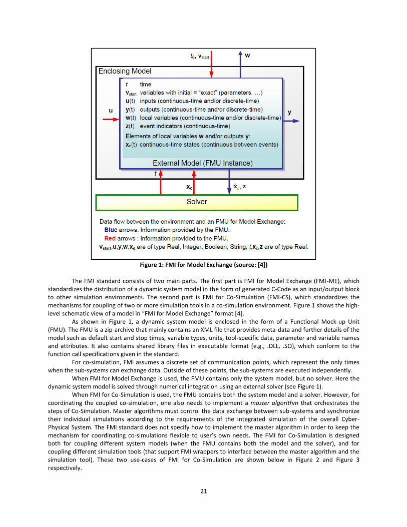
21

Figure 1: FMI for Model Exchange (source: [4])

The FMI standard consists of two main parts. The first part is FMI for Model Exchange (FMI-ME), which

standardizes the distribution of a dynamic system model in the form of generated C-Code as an input/output block to other simulation environments. The second part is FMI for Co-Simulation (FMI-CS), which standardizes the mechanisms for coupling of two or more simulation tools in a co-simulation environment. Figure 1 shows the high-level schematic view of a model in “FMI for Model Exchange” format [4].

As shown in Figure 1, a dynamic system model is enclosed in the form of a Functional Mock-up Unit (FMU). The FMU is a zip-archive that mainly contains an XML file that provides meta-data and further details of the model such as default start and stop times, variable types, units, tool-specific data, parameter and variable names and attributes. It also contains shared library files in executable format (e.g., .DLL, .SO), which conform to the function call specifications given in the standard.

For co-simulation, FMI assumes a discrete set of communication points, which represent the only times when the sub-systems can exchange data. Outside of these points, the sub-systems are executed independently.

When FMI for Model Exchange is used, the FMU contains only the system model, but no solver. Here the dynamic system model is solved through numerical integration using an external solver (see Figure 1).

When FMI for Co-Simulation is used, the FMU contains both the system model and a solver. However, for coordinating the coupled co-simulation, one also needs to implement a master algorithm that orchestrates the steps of Co-Simulation. Master algorithms must control the data exchange between sub-systems and synchronize their individual simulations according to the requirements of the integrated simulation of the overall Cyber-Physical System. The FMI standard does not specify how to implement the master algorithm in order to keep the mechanism for coordinating co-simulations flexible to user’s own needs. The FMI for Co-Simulation is designed both for coupling different system models (when the FMU contains both the model and the solver), and for coupling different simulation tools (that support FMI wrappers to interface between the master algorithm and the simulation tool). These two use-cases of FMI for Co-Simulation are shown below in Figure 2 and Figure 3 respectively.

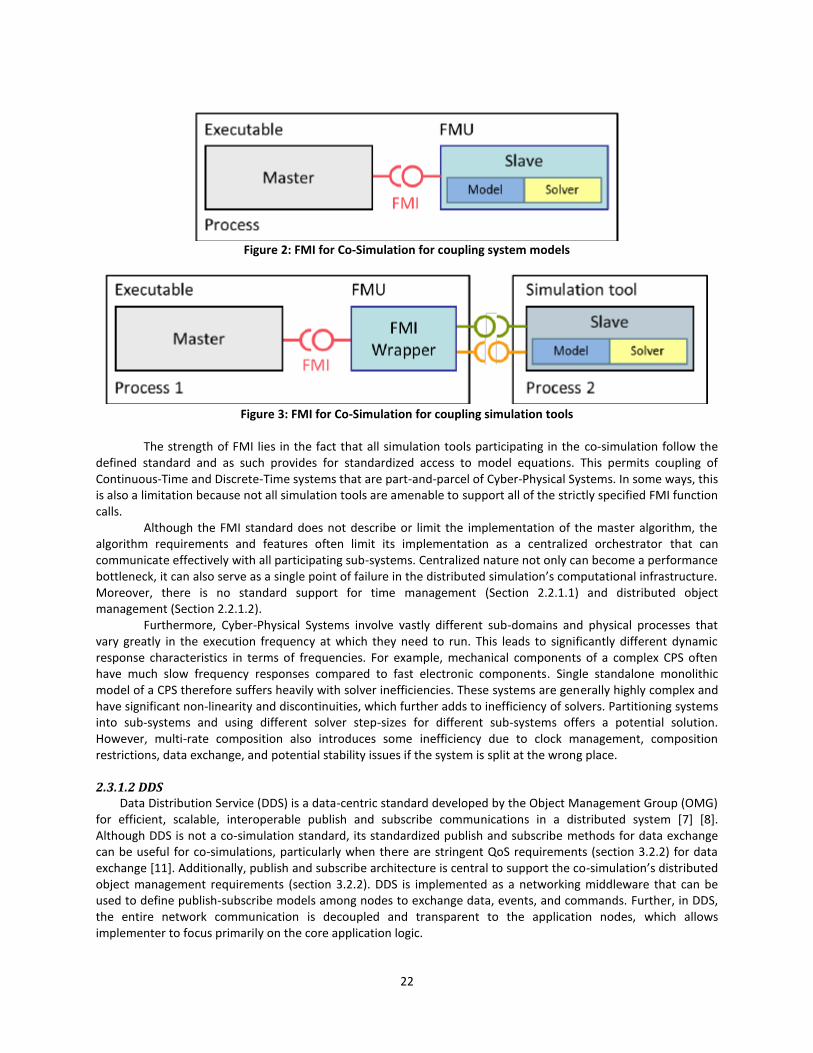
22

Figure 2: FMI for Co-Simulation for coupling system models

Figure 3: FMI for Co-Simulation for coupling simulation tools

The strength of FMI lies in the fact that all simulation tools participating in the co-simulation follow the

defined standard and as such provides for standardized access to model equations. This permits coupling of Continuous-Time and Discrete-Time systems that are part-and-parcel of Cyber-Physical Systems. In some ways, this is also a limitation because not all simulation tools are amenable to support all of the strictly specified FMI function calls.

Although the FMI standard does not describe or limit the implementation of the master algorithm, the algorithm requirements and features often limit its implementation as a centralized orchestrator that can communicate effectively with all participating sub-systems. Centralized nature not only can become a performance bottleneck, it can also serve as a single point of failure in the distributed simulation’s computational infrastructure. Moreover, there is no standard support for time management (Section 2.2.1.1) and distributed object management (Section 2.2.1.2).

Furthermore, Cyber-Physical Systems involve vastly different sub-domains and physical processes that vary greatly in the execution frequency at which they need to run. This leads to significantly different dynamic response characteristics in terms of frequencies. For example, mechanical components of a complex CPS often have much slow frequency responses compared to fast electronic components. Single standalone monolithic model of a CPS therefore suffers heavily with solver inefficiencies. These systems are generally highly complex and have significant non-linearity and discontinuities, which further adds to inefficiency of solvers. Partitioning systems into sub-systems and using different solver step-sizes for different sub-systems offers a potential solution. However, multi-rate composition also introduces some inefficiency due to clock management, composition restrictions, data exchange, and potential stability issues if the system is split at the wrong place.

2.3.1.2 DDS

Data Distribution Service (DDS) is a data-centric standard developed by the Object Management Group (OMG) for efficient, scalable, interoperable publish and subscribe communications in a distributed system [7] [8]. Although DDS is not a co-simulation standard, its standardized publish and subscribe methods for data exchange can be useful for co-simulations, particularly when there are stringent QoS requirements (section 3.2.2) for data exchange [11]. Additionally, publish and subscribe architecture is central to support the co-simulation’s distributed object management requirements (section 3.2.2). DDS is implemented as a networking middleware that can be used to define publish-subscribe models among nodes to exchange data, events, and commands. Further, in DDS, the entire network communication is decoupled and transparent to the application nodes, which allows implementer to focus primarily on the core application logic.

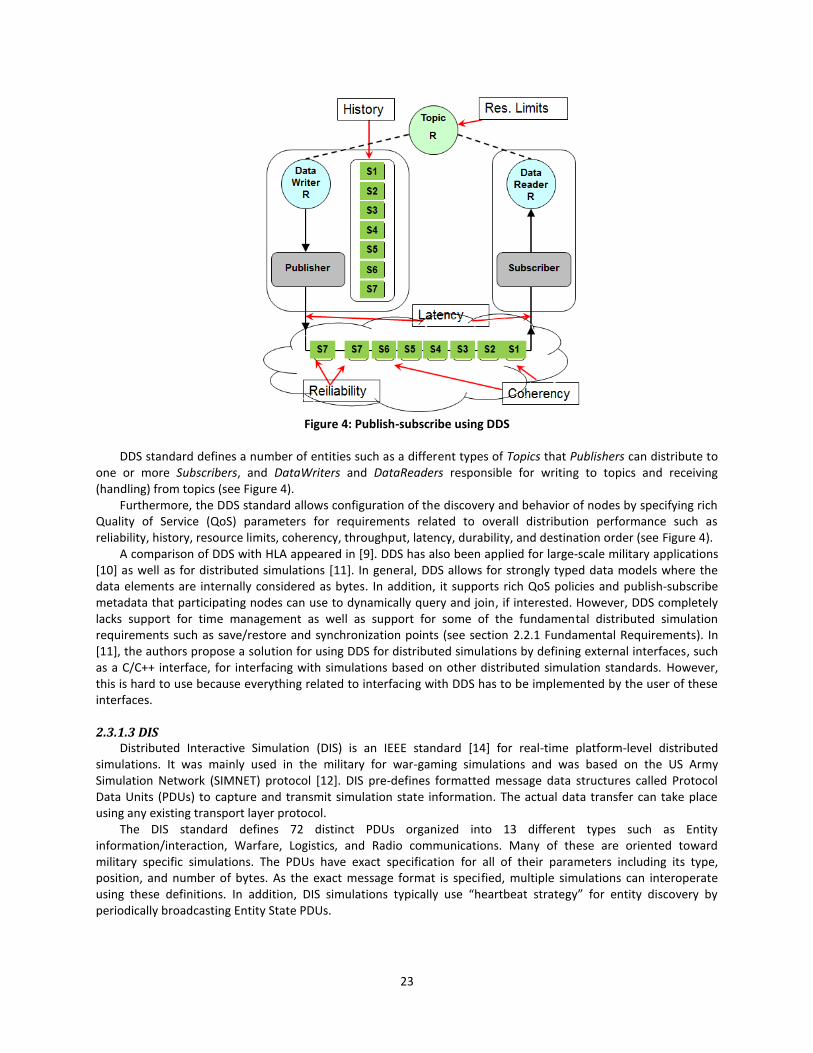
23

Figure 4: Publish-subscribe using DDS

DDS standard defines a number of entities such as a different types of Topics that Publishers can distribute to

one or more Subscribers, and DataWriters and DataReaders responsible for writing to topics and receiving (handling) from topics (see Figure 4).

Furthermore, the DDS standard allows configuration of the discovery and behavior of nodes by specifying rich Quality of Service (QoS) parameters for requirements related to overall distribution performance such as reliability, history, resource limits, coherency, throughput, latency, durability, and destination order (see Figure 4).

A comparison of DDS with HLA appeared in [9]. DDS has also been applied for large-scale military applications [10] as well as for distributed simulations [11]. In general, DDS allows for strongly typed data models where the data elements are internally considered as bytes. In addition, it supports rich QoS policies and publish-subscribe metadata that participating nodes can use to dynamically query and join, if interested. However, DDS completely lacks support for time management as well as support for some of the fundamental distributed simulation requirements such as save/restore and synchronization points (see section 2.2.1 Fundamental Requirements). In [11], the authors propose a solution for using DDS for distributed simulations by defining external interfaces, such as a C/C++ interface, for interfacing with simulations based on other distributed simulation standards. However, this is hard to use because everything related to interfacing with DDS has to be implemented by the user of these interfaces.

2.3.1.3 DIS

Distributed Interactive Simulation (DIS) is an IEEE standard [14] for real-time platform-level distributed simulations. It was mainly used in the military for war-gaming simulations and was based on the US Army Simulation Network (SIMNET) protocol [12]. DIS pre-defines formatted message data structures called Protocol Data Units (PDUs) to capture and transmit simulation state information. The actual data transfer can take place using any existing transport layer protocol.

The DIS standard defines 72 distinct PDUs organized into 13 different types such as Entity information/interaction, Warfare, Logistics, and Radio communications. Many of these are oriented toward military specific simulations. The PDUs have exact specification for all of their parameters including its type, position, and number of bytes. As the exact message format is specified, multiple simulations can interoperate using these definitions. In addition, DIS simulations typically use “heartbeat strategy” for entity discovery by periodically broadcasting Entity State PDUs.

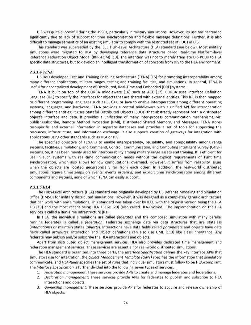
24

DIS was quite successful during the 1990s, particularly in military simulations. However, its use has decreased significantly due to lack of support for time synchronization and flexible message definitions. Further, it is also difficult to manage semantics of an existing simulator to comply with the restricted set of PDUs in DIS.

This standard was superseded by the IEEE High-Level Architecture (HLA) standard (see below). Most military simulations were migrated to HLA by developing reference data structures called Real-time Platform-level Reference Federation Object Model (RPR-FOM) [13]. The intention was not to merely translate DIS PDUs to HLA specific data structures, but to develop an intelligent transformation of concepts from DIS to the HLA environment.

2.3.1.4 TENA

US DoD developed Test and Training Enabling Architecture (TENA) [15] for promoting interoperability among many different applications, military ranges, testing and training facilities, and simulations. In general, TENA is useful for decentralized development of Distributed, Real-Time and Embedded (DRE) systems.

TENA is built on top of the CORBA middleware [16] such as ACE [17]. CORBA uses Interface Definition Language (IDL) to specify the interfaces for objects that are shared with external entities. This IDL is then mapped to different programming languages such as C, C++, or Java to enable interoperation among different operating systems, languages, and hardware. TENA provides a central middleware with a unified API for interoperation among different entities. It uses Stateful Distributed Objects (SDOs) that abstractly represent both a distributed object's interface and data. It provides a unification of many inter-process communication mechanisms, viz. publish/subscribe, Remote Method Invocation (RMI), Distributed Shared Memory, and Messages. TENA stores test-specific and external information in separate databases and provides a set of tools for supporting the resources, infrastructure, and information exchange. It also supports creation of gateways for integration with applications using other standards such as HLA or DIS.

The specified objective of TENA is to enable interoperability, reusability, and composability among range systems, facilities, simulations, and Command, Control, Communication, and Computing Intelligent Survey (C4ISR) systems. So, it has been mainly used for interoperability among military range assets and training. It is efficient for use in such systems with real-time communication needs without the explicit requirements of tight time synchronization, which also allows for low computational overhead. However, it suffers from reliability issues when the objects are located geographically far from each other. In addition, the real-world distributed simulations require timestamps on events, events ordering, and explicit time synchronization among different components and systems, none of which TENA can easily support.

2.3.1.5 HLA

The High-Level Architecture (HLA) standard was originally developed by US Defense Modeling and Simulation Office (DMSO) for military distributed simulations. However, it was designed as a completely generic architecture that can work with any simulations. This standard was taken over by IEEE with the original version being the HLA 1.3 [19] and the most recent being HLA 1516e [20] (also called HLA-Evolved). The implementation on the HLA services is called a Run-Time Infrastructure (RTI).

In HLA, the individual simulations are called federates and the composed simulation with many parallel running federates is called a federation. Federates exchange data via data structures that are stateless (interactions) or maintain states (objects). Interactions have data fields called parameters and objects have data fields called attributes. Interaction and Object definitions can also use UML [113] like class inheritance. Any federate may publish and/or subscribe the HLA interactions and objects.

Apart from distributed object management services, HLA also provides dedicated time management and federation management services. These services are essential for real-world distributed simulations.

The HLA standard is organized into three parts, the Interface Specification defines the key interface APIs that simulators use for integration, the Object Management Template (OMT) specifies the information that simulators communicate, and HLA-Rules specifies the set of rules that individual simulators must follow to be HLA-compliant. The Interface Specification is further divided into the following seven types of services:

1. Federation management: These services provide APIs to create and manage federates and federations. 2. Declaration management: These services provide APIs for federates to publish and subscribe to HLA

interactions and objects. 3. Ownership management: These services provide APIs for federates to acquire and release ownership of

HLA objects.

25

4. Object management: These services provide APIs for federates to manage life cycle and state updates of owned HLA objects.

5. Time management: These services provide APIs for federates to synchronize their logical time, use timestamps for events, and for event ordering.

6. Data distribution management: These services provide APIs for sending and receiving HLA interactions and modifying and updating HLA objects.

7. Support services: These services provide APIs for accessing general simulation information.

The OMT also has two main parts called a Federation Object Model (FOM) and a Simulation Object Model (SOM). The FOM describes the data structure and inheritance hierarchy of HLA interactions and objects. It defines the set of parameters with data types for each HLA interaction class and the set of attributes for each HLA object class. It is sometimes referred colloquially as ‘the vocabulary of the Federation’.

A Simulation Object Model (SOM), for a given federate, describes the federate’s publish and subscribe relationships with HLA interactions and objects. It specifies the type of information produced and consumed by a federate and determines the appropriateness of integrating the federate in a federation.

Also, the HLA-Rules specifies ten explicit rules that the federates and federations must follow for being HLA-compliant, such as restricting the ownership of an attribute of an object instance to a single federate at any time during the federation execution.

The recent version of the standard called HLA-Evolved improves previous version in a number of ways. One of the key additions is the use of extensible XML based modular FOM/SOM that allows partitioning modules so that only needed interactions and objects are loaded and managed in federates. Another key addition is the support for smart update rate reduction, which basically allows for updates to be delivered less frequently than the rate at which they are generated, which can significantly improve runtime performance.

The time management services are one of the key HLA services that are necessary for synchronized distributed simulations. Federates internally maintain their own internal logical time, which they can choose to synchronize with the RTI time or wall-clock or both or none. This also enables one to create real-time distributed simulations. Further, each federate can be time-regulating if their time controls time-progression of all time-constrained federates, time-constrained if their time is controlled by time-regulating federates, or both time-regulating as well as time-constrained, or neither time-regulating or time-constrained. This provides significant flexibility in designing time-synchronization among simulators varying from no time synchronization to full time synchronization, where all federates run in lockstep manner. The default implementation assumes that for real-time (wall-clock) synchronized simulations, all time-regulating federates can run faster than real-time so that they can be slowed to synchronize with the real time.

The HLA standard also allows timestamping of events and specifies different ordering methods such as timestamped-order or receive-order. It also specifies different delivery methods such as reliable delivery or best effort delivery. The key difference between the two methods is that with reliable delivery, a message will definitely be delivered, whereas with best-effort delivery, the message will be carried with best effort, but there is no guarantee that it will be delivered. However, as reliable delivery uses various network protocols for guaranteeing delivery of messages, it could involve large propagation delays, which in turn could increase runtime of the overall simulation. On the other hand, best-effort delivery can be faster to execute, but it could lead to some lost messages. Thus, there is a tradeoff between using reliable or best-effort message delivery methods.

The HLA standard is the first major generic standard for distributed simulations and provides rich set of services that are essential for creating, executing, and managing real-world simulations. With dedicated services such as federation management and time management, HLA-based simulations can be more tightly controlled and can be executed in a more time-consistent manner. The event timing, ordering, and delivery specification are unique to HLA. A number of implementations exist in both the open-source and commercial domain such as Portico RTI [21], Pitch RTI [22], and Mak RTI [23].

The HLA specification, however, does not specify a wire protocol for specifying the data structures that will be transferred over the wire between federates using a transport protocol. Different RTIs use their own implementation of the wire protocol. For example, the Portico RTI uses a communication protocol developed using JGroups [24] – a Java based multicast messaging framework. As such, the HLA does not provide means to enable security of communication among federates. Another limitation of HLA is that it does not support many of the

26

Quality of Services (QoSs) that are needed for reliable networking among simulators that are geographically separated far from each other, or involve large number and sizes of real-time data exchanges.

Some efforts to interoperate other standards with HLA have been made as in [11] [13], but these methods are not practical for real-world distributed simulations, which have complex requirements of flexibility, scalability, and customizability.

2.3.1.6 WebLVC

The Web-based Live, Virtual, Constructive (WebLVC) is an emerging protocol that relies on HTML5, WebGL, and WebSockets to enable web-applications to connect and interoperate with many different distributed simulation protocols such as HLA and DIS (see [25]). All messages in WebLVC are encoded as JSON (Java Script Object Notation) objects, which are exchanged between clients and servers using WebSockets. To interoperate with other distributed simulation protocols, such as HLA, WebLVC uses a WebLVC server that participates in the federation as a mapper for WebLVC client(s). The WebLVC server performs mapping translations between JSON objects and federation protocol specific message types (e.g. HLA interactions in case of HLA).

As WebLVC relies on generic WebSockets for communication between federations and web-applications, it enables a novel set of use-cases where a large set of diverse hardware systems are integrated and/or remote training exercises are conducted. The communication could also employ web-based authentication sessions and go across firewalls. However, the coupling is largely loose with no time management between web-applications and federations. In addition, the protocol has not been standardized yet (i.e., exists currently only as an initial draft). Further, none of the open-source RTIs fully supports it yet.

2.3.2 Frameworks and Methods for Co-Simulation

Distributed simulation problems have been studied for several decades. As a result, several standards have emerged (see Section 2.3.1 above) that attempt to fulfill some of its unique requirements. Similarly, a number of frameworks and approaches have been developed in the past for distributed simulations. We review some of these in the sections below.

2.3.2.1 FMI-Based Co-Simulation

We previously discussed the details of the Functional Mockup Interface (FMI) standard and how it specifies multiple ways of creating FMI-based co-simulations (section 2.3.1.1 FMI). Many simulation tools now support exporting and importing of models as Functional Mockup Units (FMUs). These tools need to implement a master algorithm to connect and control these FMUs while resolving the dependencies among shared variables. For example, in Dymola [27] – a Modelica based dynamics simulation tool – multiple FMUs can be connected across interface model variables and the numerical solvers provided in the tool could be customized to configure the master algorithm. Similarly, in MATLAB/Simulink [28] an FMU Toolbox enables connecting existing model blocks with FMUs.

The FMI standard does not specify how the master algorithm must be implemented or work. It also does not provide methods for time management among FMUs. Therefore, the results of co-simulations using FMI are heavily dependent on how the master algorithm is implemented and used. This is also inflexible for existing simulations that do not easily wrap as FMUs. Some frameworks do provide simplified implementation of master algorithms to enable co-simulations, but many of these are not very general.

2.3.2.2 Mosaik

The Mosaik [29] is a flexible co-simulation framework developed mainly for smart-grid simulations. It has been developed in Python. It provides an API to create scenarios and manage simulator processes. It also allows simulators to connect to a running simulation dynamically. It relies on a Python based Discrete EVent System Specification (DEVS) engine called SimPy [30] to coordinate simulators. It also provides a Java API for connecting external simulators.

Although the framework can support real-time simulations as well as event-driven as-fast-as-possible simulations, one of the fundamental issues with it is that it does not support synchronized time-stepped simulations (as fast-as-possible). Secondly, there are no explicit time management services for event timestamping or ordering. In addition, it does not have explicit support for distributed data management. The framework was

27

developed mainly for smart grid applications to support real-time simulation requirements of hardware-in-the-loop simulations. It also provides interfaces based on IEC standards for electric power systems. However, the lack of common distributed simulation services (such as those supported by HLA) makes it somewhat inflexible. Moreover, the framework only provides programming language APIs, but no graphical modeling tools or automated code generation, build, deployment, and execution capabilities.

2.3.2.3 The Ptolemy Project

Ptolemy II [31] is modeling and simulation tool developed at University of California, Berkeley and supports heterogeneous simulation integration. The primary approach used in Ptolemy tool is actor-oriented programming. The actors are concurrently executing modules that communicate with each other using ports. The novel idea used is that the actors are not necessarily atomic, but could also be composite, in that they can contain child actors. At the level at which the composite actor is present in the model, it still acts as if it is an atomic actor. Ptolemy provides implementation of a number of Models of Computation (MoCs) such as discrete event, or continuous time. These represent computational and execution semantics of the actors, and are captured as a director module inside them. Ptolemy provides special actors for different MoCs and for translation of data and events from one MoC to other. Using these, it allows for hierarchically composing actors with different MoCs to model the behavior of the entire system built using several kinds of sub-systems.

The tool is implemented in Java and is open-source. It has been used heavily for embedded systems. One of the key advantages of this tool is that by using well-defined semantics of composed actors in terms of implemented MoCs, the aggregate behavior of the composed systems can be formally analyzed. Formal verification is very important for safety-critical systems. However, as the entire system needs to be modeled using Ptolemy actors and directors, it is highly inflexible to integrate existing complex simulators. Secondly, the entire system modeled in Ptolemy is enclosed in the Ptolemy environment and is not able to interoperate with external systems. Moreover, it also does not allow dynamic addition and removal of sub-systems. Recently, an effort [32] has been made to integrate Ptolemy with HLA RTI, but is mainly a prototype extension of Ptolemy to be able to connect as HLA-federate.

2.3.2.4 FNCS

The Framework for Network Co-Simulation (FNCS) [33] was developed at Pacific Northwest National Laboratory for co-simulations of networked smart-grid applications. FNCS relies on a distributed messaging using ZeroMQ – a decentralized messaging framework [34]. Using ZeroMQ sockets, multiple applications running across different platforms can communicate with each other. FNCS provides additional facilities to optimistically synchronize time across applications and manage co-simulations. The current implementation supports a variety of power-grid simulators such as GridLAB-D [35] and EnergyPlus [36] as well as ns-3 [37] for integrated communications network simulations.

The loose coupling used in FNCS allows different time scales to be used in different simulators. The network simulation is used to send price and control power signals over a simulated network. The architecture of FNCS is more dedicated toward power systems and not primarily intended as a general architecture for co-simulations with any simulation tool. Further, the focus is more on message delivery using ZeroMQ sockets, rather than having timestamped messages and configurable event ordering methods. Moreover, the co-simulation APIs is not part of a distributed co-simulation standard, but rather custom developed and geared more toward needs of networked power simulations. Lastly, the framework is not model-driven and the support for network simulation through ns-3 is not extensive.

2.3.2.5 Parallel/Coupled DEVS

The Framework for Modeling and Simulation uses coupling of many Discrete Event Simulators is based on DEVS formalism [39] that divides the modeling and simulation exercise into 3 distinct objects. This includes the model that specifies a set of instructions (called model’s structure) for generating data and defines the behavior of the model as the set of all possible data that these instructions can generated when executed as specified. The second object is the simulator, which executes the model’s instructions that in-turn leads to the model’s emergent behavior. The third object is an experimental frame, which serves as a context in which the model is created, executed, and evaluated. The experimental frame also becomes a source of data for the simulated models. The fundamental idea of parallel DEVS is that the experimental frame can itself be formulated as a model according to

28

the DEVS formalism. This is used to provide modularity and structural composition of DEVS simulations to existing larger integrated simulations.

Parallel DEVS and the DEVS formalism provide an extensive theoretical background on composing simulations as well as on how different time-continuous and time-discrete simulators can be adapted to the DEVS formalism. In fact, many principles of HLA were also derived from the experience with parallel/coupled DEVS. In addition, many software libraries and systems supporting the formalism have also been developed in C++ and Java. However, the currently implemented framework does not support all of the complex real-world distributed co-simulations requirements such as deployment modeling, courses of action, distributed object management, time regulation, and federation management (see Section 2.2 for a discussion of real-world distributed co-simulation requirements).

2.3.3 Summary

This section reviewed a number of standards as well as framework and methods that have been developed to support distributed co-simulations. As discussed in the sections above, different standards have different goals, advantages, and disadvantages particularly when trying to apply them to distributed co-simulations of large real-world systems. For example, some standards such as FMI do not take the holistic approach needed for managing the entire integrated simulation. Similarly, many frameworks such as FNCS do not take advantage of well-defined distributed simulation standards. Also, many platforms, such as Mosaik, that are based on message-oriented frameworks, such as ZeroMQ, do not provide broad tool support for fundamental requirements of realistic distributed simulations such as modeling, code-generation, deployment, execution, and analysis. Additionally, non-reliance on standards and model-based tools makes these frameworks and approaches error-prone and hard to debug, maintain, and generalize to a variety of simulators. Finally, many testbed and frameworks such as FNCS or EPIC [40], are designed for dedicated application domains, for example FNCS for networked power systems simulations and EPIC for integrating CPS simulators with Emulab [41].

In general, instead of ad-hoc or custom approaches, standards-based integration is preferred because it is more analyzable and provides a well-defined method for integrating different simulators. Standards also specify standardized methods for exchanging data and models among simulators. The generic APIs and rules specify clear method of how different simulators need to work in compliance with the standard. Also, debugging the distributed simulation for fixing errors (albeit a highly difficult task) is easier with clearly defined rules in the standards as compared to when ad-hoc or custom approaches are used. Further, model-based framework with rich semantics are better suited for automating many of the integration tasks as well as to provide a better platform for analysis tools for distributed co-simulations.

2.4. Ontologies for model composition

2.4.1 Introduction

The independent systems of a SoS may use models developed using different modeling languages and in different simulation tools. More importantly, these models usually rely heavily on existing model libraries in the simulation tools. These model libraries contain models developed through many years of testing and validating. Therefore, it is not worth the effort to translate the models to a common language, rather an integration environment is needed to compose these disparate models to create an integrated distributed simulation.

Integration of various simulation tools can be done by defining a common data model that each of the tools agree upon and use for sharing input and output messages among them. Often, this is usually not possible for several reasons. First, the sources of a simulation tool could be unavailable (i.e., it is available only in a binary format with or without an API to control its execution). Thus, it is not possible to use an externally defined common data model. Therefore, this usually requires a translation between commonly agreed upon data model and the format of the messages that the simulation tool can understand and generate. Secondly, the sources may be available, but it may be too cumbersome to modify them to perform the back and forth translation. The simulation tool may allow some level of configuration of its input and output ports, but require substantial source code changes to write custom business logic of mapping (and aggregating/disaggregating) messages in common data model to its internal data structures. Furthermore, modifying simulation tool’s sources not only requires

29

recompiling them, but also requires source-code modification every time the integration model (containing the common data model) is updated. This incurs cost of testing and debugging the updated simulation code. For these reasons, it is desirable to separate the translation logic (called mappings) from the core simulation source-code. Therefore, we argue that:

“The translation logic should not be mixed in the core application logic in the simulation tools because it is more time-consuming to write and debug the modified main simulation code, the approach is inflexible for changes/reuse in different applications domains and models, it cannot support integration with multiple simulation tools used in the SoS, and it is an error-prone approach that is hard to maintain.”

The above observation is true for both when the translation code resides adjacent to the core simulation

code in each of the simulation tools or resides for some or all simulation tools in a separate intermediary simulation (called a mapper). Note that this is closely related to the techniques for translating/matching database schema from one format to the other, which may include pattern-based matching at different hierarchical levels of schema concepts as well as language- and constraint-based matchers [94]. However, in a mapper, the translation could also depend on the content of the messages mapped. Further, database schema translation usually supports only one-to-one, one-to-many, and many-to-one translations, whereas in a mapper many-to-many translations may also be needed.

Engineering of these mappings is also rather challenging. To begin with, one could allow specifying only a simple mapping type from the one of the output types of one simulation tool to one of the input types of another simulation. However, the real-world distributed simulations often require much greater configuration and flexibility for integration of a variety of simulation tools that are needed. A common problem is that different simulation tools may have different data models (with their own object hierarchy and attribute definitions) for representing the same type of information making it infeasible to have a direct one-to-one mapping between these data models. As an example, consider a simple sensor network in a plant and an external controller communicating actuation commands via a simulated communication network. Effectively, this requires a minimum of three simulations, viz. plant, controller, and the communication network. Here, the actuator command sent from the controller simulation to the sensor network simulation may in fact be a single message that needs to be multiplexed to all sensor nodes modeled within the sensor network model. Additionally, the topology and routing needed in the sensor network may be different from that assumed in the controller models, or it may even be, as is usually the case, completely unknown. The routing may even be dependent on the content of messages.

Another issue with direct output-input mappings is that the receiving simulation tool may differ depending on the content of the message sent. For example, in a command and control scenario, the commander may issue command messages that contain the mission aircraft identifier as an attribute. This attribute is then used to determine which simulation tool (corresponding to the specified aircraft identifier) receives this message.

Further, the translation of messages between simulation tools may require one-to-many and many-to-one mappings. One reason for this is the difference in granularity of information used in the models used in interacting simulation tools. This can be referred to as granularity difference in spatial dimension. This may require methodical aggregation and disaggregation of the information during mapping. Secondly, the interacting simulations might be operating at different time-scales – which can be referred to as granularity difference in time dimension. For example, a message may need to be communicated multiple times at each step of the receiving simulation tool (depending on how it is implemented) if its step-size is smaller than used by the sender’s step-size. Lastly, a single message from the sender may result in messages that are received periodically in the receiver. For these reasons, integration of real-world simulation tools requires one-to-many and many-to-one type of mappings. Furthermore, the use of guard condition on mappings allows for filtering messages and configuration of aggregation and disaggregation of shared information. Our observation here is:

“Integration of real-world simulation tools is better facilitated with the use of rich one-to-many and many-to-one mappings that supports specifying guard conditions for when the mappings execute to produce mapped messages. The use of these rich mappings can enable support for: (i) Variation in data structures between sender and receiver simulators, (ii) Filtering messages using guard conditions, (iii) Aggregation and disaggregation of shared information, (iv) Multiplexing

30

and de-multiplexing of information, (v) Differing time-scales in the interacting simulators, (vi) Data-dependent distribution of messages to different simulators, (vii) Data-dependent distribution of messages to different nodes within a receiver simulator, and (viii) trade-off between the level of specificity of mapped messages and the complexity of mappings needed for effective run-time message translations.”

Also, it is a highly impractical approach to manually encode the needed mappings directly in the individual

simulations as this is time-consuming, inflexible toward changing the mappings, non-reusable for mappings between other simulation tools, and highly error-prone. Therefore, we argue that:

“A model-based approach to specify the mappings that can automatically translate into executable mapping code can provide benefits of a reusable technology as well as of automated error-checking by use of constraints and generic unit tests. This can also help eliminating errors even before executing the simulation.”

Another challenge in distributed simulations is to increase the level of automation in integrating different

simulation tools. As detailed in earlier sections, composing different simulations is highly complex and needs fundamental reasoning of execution semantics of the tools for any automated composition.

Ontologies [42] provide a good way to describe, for a given domain, key concepts and the relationships among them. Ontologies have been around for more than two decades now [43], but only recently have gained popularity for their capability to capture large knowledge base of semantic information and for their applications to Artificial Intelligence (AI) and targeted search algorithms, for example [44].

A well-known formalism called Description Logic (DL) [42] is at the core of ontologies. In DL, an application domain is modeled using concepts, individuals, and roles. Concepts represent a class of things that have common set of characteristics, individuals are objects in the application domain belonging to one or more domain concepts, and roles are relationships between two individuals. The description logic modeling elements can represent a large degree of knowledge needed to map effectively between different simulation tools. Therefore, we argue that:

“Ontologies can effectively capture a large knowledge base of semantic information needed to interface and integrate different simulation tools and this knowledge base can facilitate a greater automation in ‘intelligent’ ontological rule-based model composition.”

In this section, we briefly survey some of the existing mapping techniques for model and tool integration

and evaluate their applicability for automated model composition. We also summarize the features of these techniques and present the unique challenges that are faced in the automated model composition in real-world simulations. Finally, we propose novel techniques for automated model composition using model-based configurable mapping rules and ontology-based selective knowledge capture.

2.4.2 Background on ontologies

Ontologies have been used heavily in the Artificial Intelligence (AI) area, particularly for knowledge representation of entities and facts. Over the last two decades, there has been a continual evolution in developing their syntax and semantics as well as tools to work with them. In this section, we provide a brief overview of the syntax and semantics of ontologies, the use of ontologies in different application domains, the tools and libraries available for them, and different ways in which they are used.

The basic idea behind ontologies is to capture domain knowledge systematically. The knowledge captured using ontologies includes the concepts that belong to the domain and the relationships that exist between those concepts. Ontology languages such as Knowledge Interchange Format [45] were developed in 1990’s. However, the move toward Semantic Web [46] in recent decades has fueled the drive to structure and organize the domain knowledge to make it easier to index, search, use, and interoperate. Initially, the Semantic Web used HTML and Extensible Markup Language (XML) and web technologies to support interoperability across the web. This led to the development of Resource Description Framework (RDF) [47] that defines a stack of web technology layers to define the vocabularies used and enable interoperation across the web using these vocabularies and semantics of

31

the technology layers. For example, the primitives-layer is used to define the vocabularies, and the relational layer is used to maintain consistent use of the XML datatypes in the transport layer. The Web Ontology Language (OWL) [48] was developed to address the needs of clarity, organization, and metadata reasoning required of the Semantic Web. The work started as part of the Semantic Web research started by DARPA in the form of a DARPA Agent Markup Language (DAML) [49]. This was later combined with European Union’s Ontology Interface Layer (OIL) and then picked up by the World Wide Web Consortium (W3C) to develop OWL.

The basic components of ontology are Individuals, Properties, and Classes. A class defines a group of individuals that share the same properties and so belong together. Individuals are instances of classes. Properties are binary relations between individuals or an individual and a data value. In OWL, the superclass of all classes (acting as a default class of all individuals) is called as Thing. In addition, a class that has no instances and is a subclass of all classes is called Nothing. For a detailed discussion of ontology syntax and semantics, the reader is referred to the OWL guide [51].

The OWL language comes in three flavors: OWL-Lite, OWL-Description Logic (OWL-DL), and OWL-Full. The differences between these flavors arise due to the restrictions that are placed on the use of Classes and Property types. For example, OWL-Lite and OWL-DL does not support metamodeling, while in OWL-Full the ontology constructs can be augmented or redefined. Also, only OWL-Full provides compatibility with RDF documents. Further, in OWL-Lite the cardinality constraints can only support binary values for “has” and “does not have”, whereas in OWL-DL and OWL-Full cardinality of greater than one is supported. Software tools and libraries exist for creating and analyzing ontologies such as Protégé [50] and JENA ontology API [52]. Both of these tools provide APIs to programmatically build and analyze ontologies as well as to invoke reasoners to draw inference from them.

OWL does not directly support inequalities e.g. a > b or a = b * 3. This is important in the context of modeling and simulation that rely on ontologies to capture datatypes used in its dataflows. An extension to OWL called the Semantic Web Rule Language (SWRL) [53] can be used. SWRL combines OWL’s Description Logic with a variant of RuleML (a Rule Markup Language) [53]. This enables SWRL to support logic clauses to write rules. Use of ontologies for modeling and simulation is not new. In the next section, we review some of the ways in which ontologies have been used for simulation integration, however, two patterns clearly emerge. In ontology-first approach, an all-encompassing ontology for the concepts used in all of the simulations and their interaction is first developed, and then the focus is on aligning the individual simulators to conform to this ontology. On the other hand, in ontology-last approach, the simulation models are first built (or they already exist). Ontology is then created for the domains that need to be composed and the models are augmented to map to this ontology. The advantage of the ontology-first approach is that it forces stricter agreement among the interacting simulations, which, if supported, can be easier to maintain. However, these ontologies tend to be too general and quickly become cumbersome and unwieldy for large real-world systems because of their highly heterogeneous nature (see section 2.2). On the other hand, creating ontology after the models have been created is relatively easier, but ensuring that the models map to the ontology accurately is difficult. However, the advantage of ontology-last approach is that this is applicable, scalable, and manageable even for very large real-world systems.

Use of ontology for interoperability of systems could be syntactic, semantic, or pragmatic. The syntactic interoperation uses ontological terms to map one-to-one domain interactions directly. This is the lowest level of interoperation. The higher level of interoperation is semantic. Here the ontological concepts are tied using mapping rules that are derived from the semantics of the ontological concepts in their respective domains. This is a more effective way of enabling interoperation, and requires less amount of information exchange than at syntactic level. However, it requires knowledge, methods, and tools to enable semantic mappings. The highest level of interoperation is pragmatic, which requires the minimal amount of information exchange but requires complex logic and infrastructure to create and execute mappings for interoperation.

2.4.3 Related Work

Ontologies have been mainly used for knowledge gathering and data mining through artificial intelligence rules. In the past several years, interest has developed in using ontologies for modeling and simulation. In this section, we review some of the prominent efforts for simulation integration using ontologies. We arrange the review in four categories viz. syntactic port mapping for interconnected simulations, ontology-based frameworks for modeling and simulation, domain-specific ontologies for simulation, and approaches for bridging HLA and DIS.

32

2.4.3.1 Syntactic port mapping for interconnected simulations The first proposal for using ontology for software composition was developed by Gio Widerhold in [54],

which argues that in order to compose large-scale software an agreement must exist about the terms used. The reasoning was that as the models depend on symbolic linkages among the simulations and the agreed upon terms can be used to create a domain-specific software architecture that supports software composition. It also developed an object-based structural algebra across multiple domains and algebraic operations to relate these domains. This work provided a good theoretical background. However, it did not develop the tools and methods needed for executable compositions of complex real-world systems.

In 2003, Vei-Chung Liang proposed [55] to use direct port mapping to compose models. It defined ports as the locations of interactions at the boundaries of the simulations to create a modularized and encapsulated component that can interact with other modular components with matching ports. It builds port ontology to define many port types to broaden the domains that can be captured using this approach. However, this approach is not well suited for modeling and simulation as the mapping between different simulations is not always one-to-one and requires transformation across domains. It also does not support automated model composition.

A proposal to use ontologies for modeling and simulation was developed by John Miller in 2004 [56]. It developed a Discrete Event Modeling Ontology (DeMO) to capture events and timing of discrete event systems. It proposed to use this ontology to create models (ontology-first) so that they take inputs and generate outputs only using the terms in the ontology and further proposed to use the commonly agreed ontology to facilitate knowledge exchange between different domains. It used Extensible Stylesheet Language Transformations (XSLT) to map messages across domains. However, the real-world systems are highly heterogeneous and require complex mappings and rules to compose models that are not amenable to simple XSL transformations.

Another prominent work in this area was presented as part of the doctoral thesis by Lee Lacy [57]. This work developed a Process Interaction Modeling Ontology for Discrete Event Simulations (PIMODES) and provided proof-of-concept translations from simulation models to and from PIMODES. It also demonstrated interchanging models across domains. However, real-world model composition requires deeper transformation logic as well as automated model composition rules to map cross-domain models.

2.4.3.2 Ontology-based frameworks for modeling and simulation

An ontology-based approach was proposed in 2007 by Perakath, et al. [58]. In this approach, they argue that using an ontological development to gather domain knowledge can effectively reduce inefficiencies due to ambiguous specifications. They proposed a well-defined method to go from system description to a conceptual system model and then to a formal ontological specification for corresponding simulation. The ontologies are then used for analyzing and validating the system. They also include a brief survey of the application of ontologies for distributed simulations and multi-level abstractions modeling. Using these concepts, they developed an ontology-based framework for simulation modeling and analysis. However, this represents a usual ontology first paradigm, where the system to be integrated has pre-determined system-specific ontologies. In the real-world simulations, however, the ontologies should be determined by the simulation models and the nature of integration.

The use of Web Ontology Language (OWL) for modeling and simulation was developed by Lee Lacy in PhD dissertation [57]. As described above, the primary focus of this work was on interchanging models. The simple translations of simulation models to the common DEVS ontology are not easily applicable for many real-world simulation tools that have complex behavioral patterns of event handling and system and time progression. Real-world distributed co-simulations require complex mappings across different domains and applications.

2.4.3.3 Domain-specific ontologies for simulation

Over the past several years, the ontologies have been increasingly used in many different domains. Many of these ontologies focus on enabling unambiguous means of knowledge gathering and communication. For example, [59] presents a highly detailed ontology for communication networks, while [44] develops a specific ontology for scientific texts. In addition, ontologies have been used for Service-Oriented Architectures (SOAs) and composition through ontological description of web-services [60].

2.4.3.4 Mapping approaches used for bridging HLA and DIS

As described previously, DIS and HLA are widely used distributed simulation standards, but distributed simulation communities are moving toward using HLA as the older DIS standard provides only a limited set of

33

functionality. However, a large set of highly valued rich models (and simulations) already existed based on DIS and re-writing them was both technically as well as economically prohibitive. The HLA standard does not require using a particular Federation Object Model (FOM), but requires that one must be created that is shared among all federates that are part of a corresponding federation. Therefore, in 1999, a fixed FOM equivalent to the data models of DIS was developed. This was called the Real-time Platform-level Reference FOM (or RPR-FOM) as part of a SISO standard, SISO-STD-001.1-1999 [13]. The idea was that the legacy applications based on DIS could be easily targeted to support RPR-FOM, which had similar data structures, as opposed to any FOM that a federation designer might use. As a corollary, this forced modelers in other simulation tools to use the same FOM and develop their logic around that fixed FOM. Obviously, this is highly sub-optimal and often impractical. A technique was needed to let developers use their own FOMs, but somehow still be able to talk to each other.

A tool called GMUGateway [61] was developed by George Mason University for automated mapping between DIS-HLA. It used an XML based initialization-time configuration to represent DIS PDUs as HLA-objects and implemented functionality to convert from between the two. This enabled easier bridging between HLA and DIS based simulation tools. In addition, in the commercial domain, the popular RTI called Mak [23] provided a VR-Link module [23] to connect DIS and HLA. Later Mak also developed a generic VR-Exchange module [23] that performed FOM-to-FOM translation, bridging between multiple RTIs and distributed simulation standards.

2.4.4 Summary of current ontological approaches in simulations

As described in earlier sections, ontologies have been developed and used for different applications. Several ontologies were developed for unambiguous knowledge gathering and communication for specific application domains such as communication networks, web-services, and medical textual notes [44] [59] [60]. Several approaches have been developed to apply them for systematic simulation creation [58] and integrating different simulation tools [54] [55] [56] [57]. Much of the existing work focus on ontology first paradigm, which tries to comply different simulation tools to a universal ontology. However, as Kreutzer [64] showed in 1986 that it is impossible and impractical to create a simulation language that supports universal model interchange. Therefore, we need a paradigm where models pre-exist and ontologies are created in a domain-specific manner and a comprehensive approach for mapping across different domains.

Current approaches, such as in [55], focus on one-to-one mapping across input-output ports and ignore the internal structure and semantics of composed models. However, for real-world model composition a number of unique requirements must be supported. For example, the data sent by a sender may need to be post-processed by the orchestrator before delivering it in appropriate format to the receiver. Additionally, not all data exchanges in one model may result in corresponding messages in other model depending on domain-specific filtering requirements. Even the interacting models representing different aspects of the same system may vary in degree of fidelity. This can result in situations that the data producers in one model may not have corresponding data receivers in the other model and vice versa. Moreover, the model of data distribution could vary between point-to-point to broadcast in different models. An example of this could be that, in an organizational model, the data exchange between nodes may carry operational commands, which in the corresponding communication network model may need to be replicated through many multiplexed network messages to all nodes in the receiving organization. Another variation of this requirement is that in one model the data might be sent via direct logical channels, which in a communication network may require the use of complex network routes as well as transport, routing, and other protocols. Finally, a message exchange between nodes in one model may correspond to a complex iteration of message exchanges between nodes in another model. For example, in a logical domain, the message may be simply to send a negotiated price, but in a corresponding high-fidelity negotiation simulator, the full negotiation must be orchestrated through the necessary iterations between nodes, which in-turn may result in many different network messages in a corresponding network simulator.

Considering the various complex use-cases described above that arise in real-world model compositions, it becomes a tradeoff between how fine-grained the ontology for model composition is created versus how flexible the model composition process is for composing many different types of models.

34

CHAPTER 3. RESEARCH PROBLEMS AND HYPOTHESIS

3.1 Research Problems

For real-world simulation integration and experimentation, it is not sufficient to concoct simply a means of co-simulating two or more simulations at hand. Instead, a well-defined and model-based integration approach is needed. This requires a comprehensive framework that supports critical aspects of real-world integrated simulations, such as integration modeling, model composition, parameterization, experimentation, and analysis. We recognize the following research problems:

1. How can we create an integrative framework that supports model-based distributed simulation and its

fundamental requirements for modeling, configuring, and experimentation? The framework must provide a modeling language to create system integration models, generators to synthesize artifacts programmatically from the integration models to implement and configure the distributed simulation, a controller to control the distributed simulation, and tools and techniques for automated deployment of simulations on computers as well as executing them.

2. How can we support legacy simulation tools that have fixed data models for which they work? Automatic mapping techniques are needed for translating messages between the fixed data model format used by the legacy simulation tools and the common data model used by the rest of the distributed simulation.

3. How can we create a reusable component for communication network simulation that can be easily configured and reused for many different network topologies that may be needed in different distributed simulation scenarios?

4. How can we support dynamic models partitioned into separate FMUs across separate sampling rate boundaries? The framework should support FMUs as one of the simulation components and it should support executing different FMUs at different step-sizes.

5. How can we create a reusable cyber-attack library for evaluating how cyber-attacks can affect system behavior and how resilient its security mechanisms are to mitigate these effects? The library should allow selecting, configuring, and applying a variety of reusable cyber-attacks at various network elements.

6. How can we support scenario-driven experimentation to study the emergent behavior of the distributed simulation under several what-if scenarios? The required capabilities include modeling, configuring, executing, and monitoring of multiple, parallel courses-of-action.

7. How can we use ontologies for automatically compose models in different domains? For example, a road traffic simulation understands traffic flows and associated variables, but a communication network only works with network packets. In order to study the integrated system behavior, these two models must be composed together. Ontology-based tools and techniques are needed to automate this composition.

3.2 Research Hypothesis

“Model-based rapid synthesis of distributed HLA-based simulations is implementable as a reusable and integrative distributed simulation framework and can support mapping methods for legacy component interfaces, reusable component for communication network simulation, multi-rate model partitioning using FMU-CS, modeling and integration of cyber-attacks, scenario-driven experimentation using courses of action evaluation, and ontology-based model composition. Such an integrative framework should help system integrators with rapidly synthesizing distributed simulations while handling multiple of above problems as well as provide intelligent composition of models.”

35

CHAPTER 4. MODEL-BASED INTEGRATION FOR DISTRIBUTED SIMULATION EXPERIMENTS

4.1 Introduction

Real-world simulations are composed of many different systems, each with unique requirements for their evaluations, and each potentially requiring many different modeling and simulation tools depending on their requirements and functions and the corresponding simulation tools that are suited for simulating those behaviors. For example, a manufacturing plant may need to analyze the behavior of a particular machine being manufactured such as a car or an engine. Evaluation of this product may need many different simulation tools in order to simulate different aspects of its behavior faithfully such as electrical, mechanical, thermal, structural, and cyber. In addition, these systems often need to be evaluated for their interaction with hardware and humans, and for cyber communications among various system components and systems within the system.

Integrated evaluation of these heterogeneous simulation tools is a highly difficult task. Not only these simulation tools have very different modeling languages and syntax, but also their semantics are vastly different. As discussed earlier in section 2.1, there are many different sources of heterogeneity that makes the problem challenging. Successful evaluation of the system-of-systems must deal with the pervasive heterogeneity and develop techniques to make the heterogeneous models and systems work seamlessly in an integrated manner.

For the development of an integration and experimentation framework for distributed simulation experiments, one must use model-based techniques for integration modeling and automated synthesis of executable experiments. For the real-world simulation integration and experimentation, it is not sufficient to concoct simply a means of co-simulating two or more simulations at hand. The manual process not only is slow and susceptible to inadvertent variations, but also is error-prone. On the other hand, a model-based integration approach can facilitate automation for many tasks of creating, executing, coordinating, and controlling distributed simulations and thereby support rapid experimentation under a variety of test scenarios or variations of test conditions. Other potential benefits of model-based approach include reproducibility, maintainability, and traceability. However, to support model-based integration, we need a comprehensive framework that supports critical aspects of real-world integrated simulations, such as integration modeling, model composition, parameterization, experimentation, and analysis. The problem we are trying to address in this chapter is:

“How can we create an integrative framework that supports model-based distributed simulation and its fundamental requirements for modeling, configuring, and experimentation? The framework must provide a modeling language to create system integration models, generators to synthesize artifacts programmatically from the integration models to implement and configure the distributed simulation, a controller to control the distributed simulation, and tools and techniques for automated deployment of simulations on computers as well as executing them.” Owing to the rapid growth in the size and heterogeneity of systems in the last several decades, the large

system-of-systems (SoSs) have become highly complex to manage. These systems encompass many different types of systems spanning organizational workflows to cyber infrastructure to even many different engineering/physical domains with highly varying physical characteristics. These systems are usually evaluated in isolation using many different special-purpose simulation tools (specialized with many years of research) such as Matlab/Simulink [67], OMNeT++ [68], and CPN Tools [66]. However, the integrated evaluation of the SoS as a whole requires modeling the interdependencies of many of its aspects simultaneously, for example the modeling of its physical phenomenon with digital infrastructure including sensors, controllers, communication network, and software. Currently, there is no efficient way to do this using the currently available special-purpose simulators. Specifically, these special-purpose tools lack several things such as (i) integrated modeling of physical domains with communication and control system, (ii) interactions across multiple physical domains, and (iii) combining data that is multi-rate, multi-scale, multi-user, and multi-model from different domains.

Two key characteristics are typical of these large SoSs: (i) low rate of information exchange, and (ii) relaxed timing accuracy requirements on the information exchange. The rate of information exchange refers to the number of data exchange and coordination events at every time-step. For large SoSs, this is usually low (i.e., it does not grow exponentially with the number of systems integrated) because the individual systems execute

36

largely independent of others, involving only a few interactions with a rather small subset of other systems. The timing accuracy requirements refers to how close the timestamp of the exchanged data at the receiver simulator should be to the timestamp of the same information at the sender simulator. For large SoSs, again because the individual systems execute largely independently, the timing accuracy requirements are usually relaxed (i.e., range from a few seconds to even minutes). For example, a simulation of a large organization’s system for a period of 24 hours, it might be good enough for the exchanged data between its individual systems (e.g., a decision made by a decision-making process that took 2 hours to make it) to arrive within a few seconds of being generated by the sender system. It should be noted though that the approaches developed in this research are still applicable to sub-second timing accuracy requirements, but the integrated simulation may execute with increased overall runtime.

Simulation integration of these systems usually starts as one-off method for the task at-hand. However, many real-world requirements require several adaptations and extensions to existing tools and methods. Our work approaches the generalizable integration techniques at the outset for general-purpose simulation integration. Thus, simulation-based evaluation of behavior of large SoS is complex, as it involves multiple, heterogeneous, interacting domains. Each simulation domain uses its special-purpose simulation tools, but their integration into a coherent framework is a very difficult, time-consuming, labor-intensive, and error-prone task. Consequently, rapid computational studies, that are needed to provide timely answers to planners, operators, analysts, cannot be easily accomplished. In addition, these systems must be evaluated against a variety of operational scenarios and under many different test conditions, which can potentially lead to a large set of experiments that can be very hard to perform manually. Therefore, in this research we developed a model-based framework, called Command and Control Wind Tunnel (C2WT), for efficiently synthesizing large-scale integrated heterogeneous simulations.

The rest of the chapter is organized as following. In Section 4.2, we provide a brief architectural overview of our simulation integration framework. Next, we present the model-based integration approach in detail in Section 4.3. We describe the methods developed to integrate different simulation engines in Section 4.4. In Section 4.5, we show how simulation experiments are deployed on compute nodes, and how their execution is coordinated and controlled using a novel simulation manager component called the Federation Manager (FM). In Section 4.6, we discuss our approach for hardware-in-the-loop simulation. Further, in Section 4.7, we describe a non-trivial case study and present results of the experiments conducted using our framework. We present different levels of framework users in Section 4.8. Finally, in Section 4.9, we present a summary of the chapter.

4.2 Architectural Overview

The fundamental problem with existing models and simulators is that these are generally limited to specific domains and are not directly suitable for cross-domain analysis. For example, different systems of the SoS may differ in their time-scales, types of models, and level of fidelity. Here, a framework that allows analyzing these complex cross-domain interactions is needed. This framework should enable integration of domain-specific models and simulators in a logically and temporally coherent manner. Further, the framework should support experimentation and deployment capabilities for performing scalable simulation experiments. Figure 5 shows the three key layers of integration platforms in our framework:

1. Model Integration Platform: Model integration is required for expressing interactions across modeling domains - a need for multi-model simulations. The primary challenge to be addressed has been the semantic heterogeneity of domain models and the different model-types required for the specification of a simulation experiment. The fact that domain models in SoS subdomains are provided by different simulation tools that evolve more or less independently further adds to the modeling language and model integration challenge.

2. Simulation Integration Platform: End-to-end integration of simulations for a SoS experiment requires a robust distributed simulation integration framework that goes beyond the semantically weak and necessarily fragile ad-hoc connection among tools. We use the established, standard-based approach for distributed simulation integration, using the High-Level Architecture (HLA) [20] [107].

3. Execution Integration Platform: The dominant approach in current tool suites is desktop integration using platforms such as Microsoft’s Visual Studio [101], or Eclipse [102]. However, the simulation tools used for the systems of a large SoS are usually special-purpose, complex, and heterogeneous (see Section 2.1.5). Manual deployment of these simulators on compute nodes and coordination and control of their

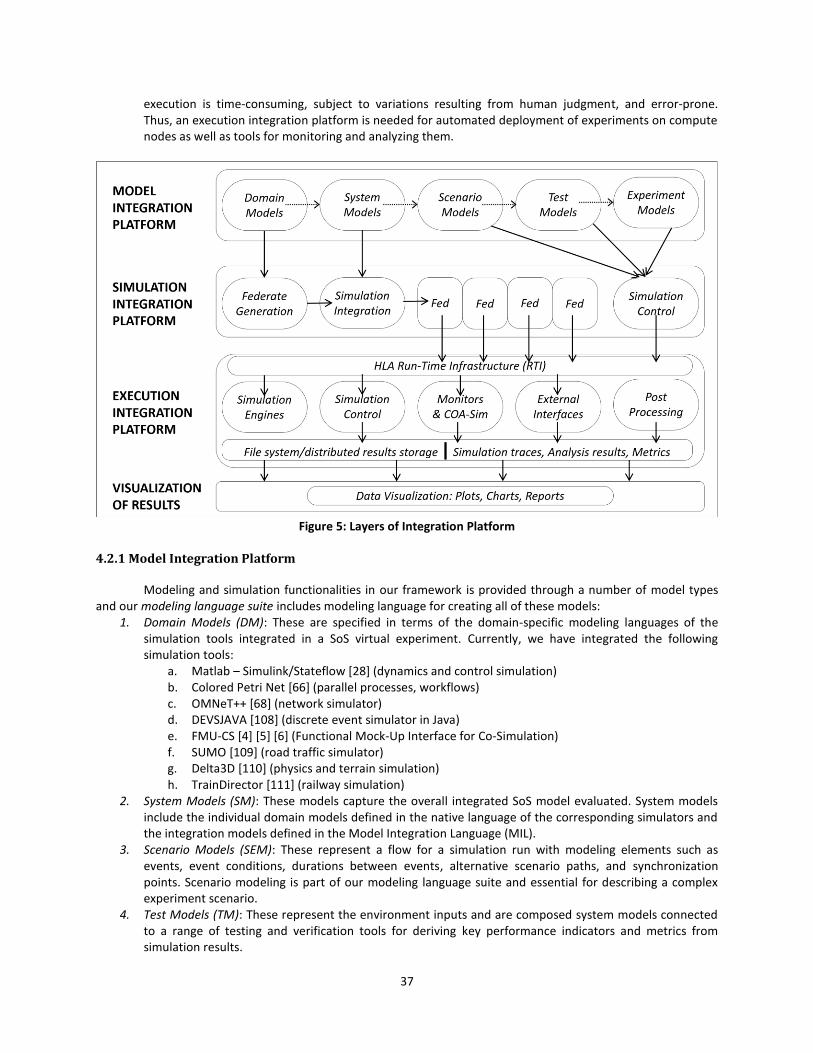
37

execution is time-consuming, subject to variations resulting from human judgment, and error-prone. Thus, an execution integration platform is needed for automated deployment of experiments on compute nodes as well as tools for monitoring and analyzing them.

Figure 5: Layers of Integration Platform

4.2.1 Model Integration Platform

Modeling and simulation functionalities in our framework is provided through a number of model types and our modeling language suite includes modeling language for creating all of these models:

1. Domain Models (DM): These are specified in terms of the domain-specific modeling languages of the simulation tools integrated in a SoS virtual experiment. Currently, we have integrated the following simulation tools:

a. Matlab – Simulink/Stateflow [28] (dynamics and control simulation) b. Colored Petri Net [66] (parallel processes, workflows) c. OMNeT++ [68] (network simulator) d. DEVSJAVA [108] (discrete event simulator in Java) e. FMU-CS [4] [5] [6] (Functional Mock-Up Interface for Co-Simulation) f. SUMO [109] (road traffic simulator) g. Delta3D [110] (physics and terrain simulation) h. TrainDirector [111] (railway simulation)

2. System Models (SM): These models capture the overall integrated SoS model evaluated. System models include the individual domain models defined in the native language of the corresponding simulators and the integration models defined in the Model Integration Language (MIL).

3. Scenario Models (SEM): These represent a flow for a simulation run with modeling elements such as events, event conditions, durations between events, alternative scenario paths, and synchronization points. Scenario modeling is part of our modeling language suite and essential for describing a complex experiment scenario.

4. Test Models (TM): These represent the environment inputs and are composed system models connected to a range of testing and verification tools for deriving key performance indicators and metrics from simulation results.

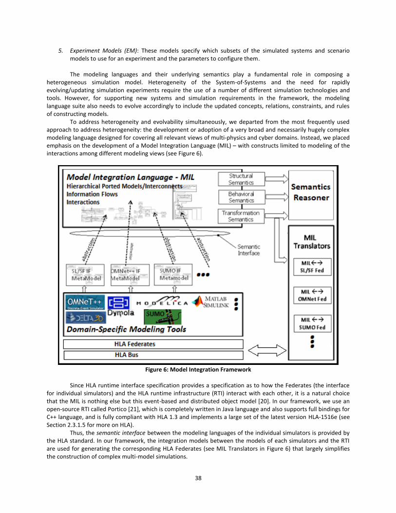
38

5. Experiment Models (EM): These models specify which subsets of the simulated systems and scenario models to use for an experiment and the parameters to configure them. The modeling languages and their underlying semantics play a fundamental role in composing a

heterogeneous simulation model. Heterogeneity of the System-of-Systems and the need for rapidly evolving/updating simulation experiments require the use of a number of different simulation technologies and tools. However, for supporting new systems and simulation requirements in the framework, the modeling language suite also needs to evolve accordingly to include the updated concepts, relations, constraints, and rules of constructing models.

To address heterogeneity and evolvability simultaneously, we departed from the most frequently used approach to address heterogeneity: the development or adoption of a very broad and necessarily hugely complex modeling language designed for covering all relevant views of multi-physics and cyber domains. Instead, we placed emphasis on the development of a Model Integration Language (MIL) – with constructs limited to modeling of the interactions among different modeling views (see Figure 6).

Figure 6: Model Integration Framework

Since HLA runtime interface specification provides a specification as to how the Federates (the interface

for individual simulators) and the HLA runtime infrastructure (RTI) interact with each other, it is a natural choice that the MIL is nothing else but this event-based and distributed object model [20]. In our framework, we use an open-source RTI called Portico [21], which is completely written in Java language and also supports full bindings for C++ language, and is fully compliant with HLA 1.3 and implements a large set of the latest version HLA-1516e (see Section 2.3.1.5 for more on HLA).

Thus, the semantic interface between the modeling languages of the individual simulators is provided by the HLA standard. In our framework, the integration models between the models of each simulators and the RTI are used for generating the corresponding HLA Federates (see MIL Translators in Figure 6) that largely simplifies the construction of complex multi-model simulations.

39

4.2.2 Simulation Integration Platform

The role of the Simulation Integration Platform is to establish the interaction across the concurrently running simulators by coordinating time advancement and routing data. Since we have chosen the High Level Architecture (HLA) as the backbone for the Simulation Integration Platform, we summarize here its background and services.

An HLA simulation is composed of a federation of individual simulation federates. Shared objects and interactions are defined to which any federate may publish or subscribe. Objects are analogous to OS-style shared memory and are owned by one federate. Interactions correspond to message passing. All federation configuration information is stored in a standardized format text file called the FED file. In theory, this configuration file is portable across different HLA run-time infrastructure (RTI) implementations.

The HLA standard advanced the flexibility of time control in an integrated simulation. Fundamentally, every federate must maintain a clock corresponding to the logical time internal to its simulation. This clock is distinct from any real-world “wall-time”. The standard provides numerous schemes for coordinating logical clock evolution among federates. These can range from completely lacking time synchronization, where one federate can execute arbitrarily far into the future, to completely synchronized, where all federates evolve time within a tightly bound window. Each federate can be configured to be time-constrained or time-regulating, both, or neither. A time-regulating federate's progression constrains all time-constrained federates. Likewise, a time-constrained federate's advance is controlled by all time-regulating federates. A federate that is neither constrained nor regulating is free to evolve time independently. Federates that are both time-regulating and time-constrained, evolve time in a tight lockstep. If, for example, all federates can run at least as fast as real-time, and one federate tightly correlates its time advance requests to wall-clock time, then the entire federation can be made to run in real-time. Otherwise, it is possible to execute simulations both faster and slower than real-time.

Each HLA federate defines a step-size, lookahead interval and minimum timestamp. When a federate issues a request to evolve its internal simulation time, it does so in increments of step-size, which may vary in size from step to step. Lookahead corresponds to the amount of time into the future, which the federate guarantees it will not issue an interaction or object update and is generally small compared to step-size. When the federate is in a Time Advance Request (TAR) state, minimum timestamp is defined as the federate's requested time plus lookahead. When the federate is in a Time Advance Granted (TAG) state, minimum timestamp is the federate's logical clock time (as the granted time could be less than the requested time) plus lookahead. It is also important to understand that each federate maintains an understanding of all of all other federate's minimum timestamps.

Figure 7, adapted from [20], illustrates how time advances happen in a federation of two time-regulating and time-constrained federates. In this example, federate A always seeks to advance its clock in steps of size s, while federate B steps are of size 3s. Wall-clock time runs to the right, but has no units to reinforce that there is no mandatory correlation between logical and wall time. Event 1 is federate A issuing a time advance request (TAR) to the HLA run-time infrastructure (RTI) to advance its logical clock by its step-size. It cannot advance its logical clock until federate B's minimum time is greater than its requested time. Event 2 is federate B issuing a TAR, which immediately causes its minimum to go to T+3s since its step-size is 3s. This allows federate A to change to Time Advance Granted (TAG) state and progress its logical clock to T+s. At events 4 & 5 and 6 & 7, federate A issues TAR followed immediately by TAG since federate B's minimum time is still greater. Finally, once event 6 has occurred, federate B can move into a TAG state and advance its logical clock. The whole sequence then begins to repeat itself.

A significant advantage of HLA over other integration frameworks such as DIS [14] and SIMNET [12] is its complete divorce of the framework from the subject being simulated. Compared to a recent simulation integration framework, Functional Mock-up Interface Co-Simulation (FMI CS) [5], HLA is significantly more complete by offering solution for the two essential problems in distributed simulation integration: time management and distributed data model.

A challenge not addressed by the HLA standard is the consequence of its flexibility. HLA-based simulation components can be moved relatively easily from one network of computers to another for development or execution. The HLA standard does not directly address this ability and leaves such functionality up to HLA implementations or integration designers.

Relevant commercial integration software between specific simulators and HLA does exist, (such as the HLA Toolbox for MATLAB federates by ForwardSim Inc. [112]), but these efforts do not have any support for

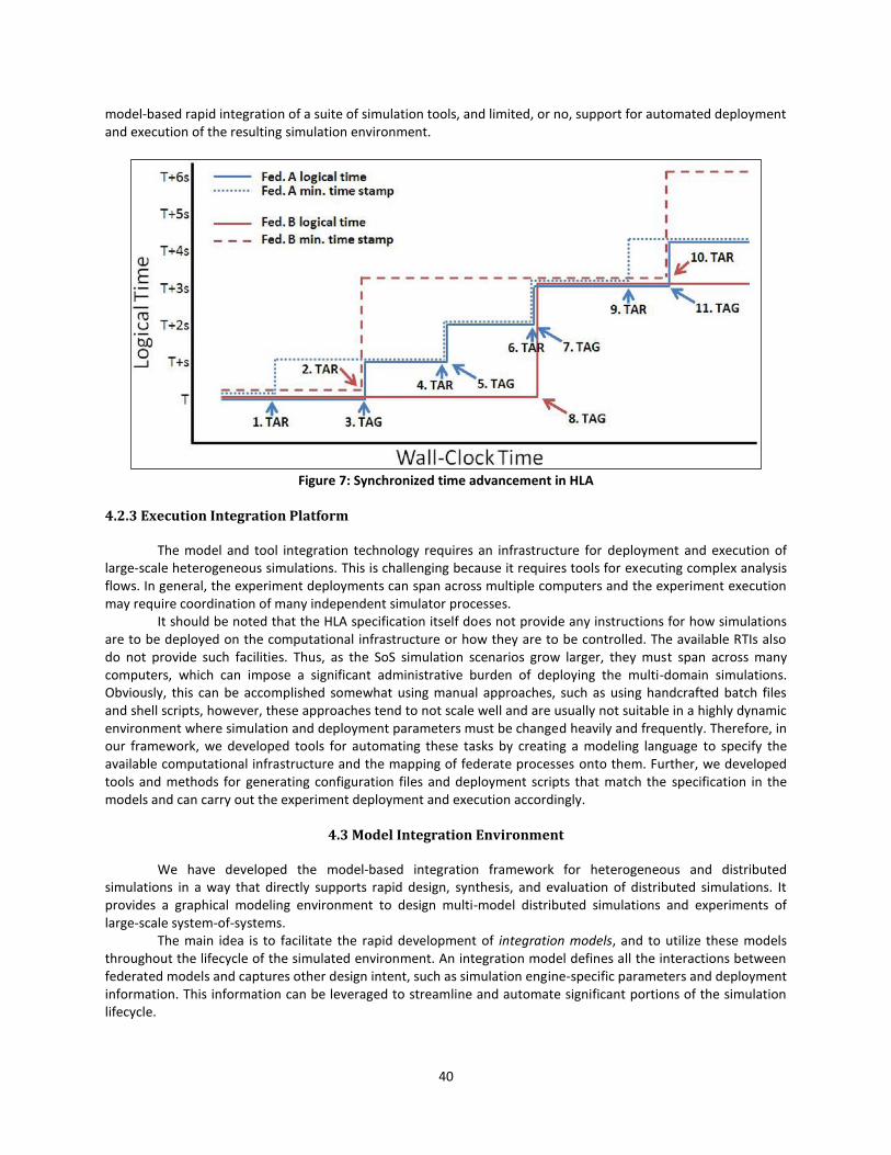
40

model-based rapid integration of a suite of simulation tools, and limited, or no, support for automated deployment and execution of the resulting simulation environment.

Figure 7: Synchronized time advancement in HLA

4.2.3 Execution Integration Platform

The model and tool integration technology requires an infrastructure for deployment and execution of large-scale heterogeneous simulations. This is challenging because it requires tools for executing complex analysis flows. In general, the experiment deployments can span across multiple computers and the experiment execution may require coordination of many independent simulator processes.

It should be noted that the HLA specification itself does not provide any instructions for how simulations are to be deployed on the computational infrastructure or how they are to be controlled. The available RTIs also do not provide such facilities. Thus, as the SoS simulation scenarios grow larger, they must span across many computers, which can impose a significant administrative burden of deploying the multi-domain simulations. Obviously, this can be accomplished somewhat using manual approaches, such as using handcrafted batch files and shell scripts, however, these approaches tend to not scale well and are usually not suitable in a highly dynamic environment where simulation and deployment parameters must be changed heavily and frequently. Therefore, in our framework, we developed tools for automating these tasks by creating a modeling language to specify the available computational infrastructure and the mapping of federate processes onto them. Further, we developed tools and methods for generating configuration files and deployment scripts that match the specification in the models and can carry out the experiment deployment and execution accordingly.

4.3 Model Integration Environment

We have developed the model-based integration framework for heterogeneous and distributed simulations in a way that directly supports rapid design, synthesis, and evaluation of distributed simulations. It provides a graphical modeling environment to design multi-model distributed simulations and experiments of large-scale system-of-systems.

The main idea is to facilitate the rapid development of integration models, and to utilize these models throughout the lifecycle of the simulated environment. An integration model defines all the interactions between federated models and captures other design intent, such as simulation engine-specific parameters and deployment information. This information can be leveraged to streamline and automate significant portions of the simulation lifecycle.

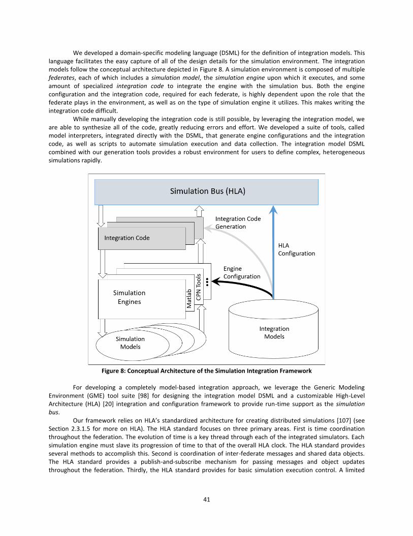
41

We developed a domain-specific modeling language (DSML) for the definition of integration models. This language facilitates the easy capture of all of the design details for the simulation environment. The integration models follow the conceptual architecture depicted in Figure 8. A simulation environment is composed of multiple federates, each of which includes a simulation model, the simulation engine upon which it executes, and some amount of specialized integration code to integrate the engine with the simulation bus. Both the engine configuration and the integration code, required for each federate, is highly dependent upon the role that the federate plays in the environment, as well as on the type of simulation engine it utilizes. This makes writing the integration code difficult.

While manually developing the integration code is still possible, by leveraging the integration model, we are able to synthesize all of the code, greatly reducing errors and effort. We developed a suite of tools, called model interpreters, integrated directly with the DSML, that generate engine configurations and the integration code, as well as scripts to automate simulation execution and data collection. The integration model DSML combined with our generation tools provides a robust environment for users to define complex, heterogeneous simulations rapidly.

Figure 8: Conceptual Architecture of the Simulation Integration Framework

For developing a completely model-based integration approach, we leverage the Generic Modeling

Environment (GME) tool suite [98] for designing the integration model DSML and a customizable High-Level Architecture (HLA) [20] integration and configuration framework to provide run-time support as the simulation bus.

Our framework relies on HLA’s standardized architecture for creating distributed simulations [107] (see Section 2.3.1.5 for more on HLA). The HLA standard focuses on three primary areas. First is time coordination throughout the federation. The evolution of time is a key thread through each of the integrated simulators. Each simulation engine must slave its progression of time to that of the overall HLA clock. The HLA standard provides several methods to accomplish this. Second is coordination of inter-federate messages and shared data objects. The HLA standard provides a publish-and-subscribe mechanism for passing messages and object updates throughout the federation. Thirdly, the HLA standard provides for basic simulation execution control. A limited

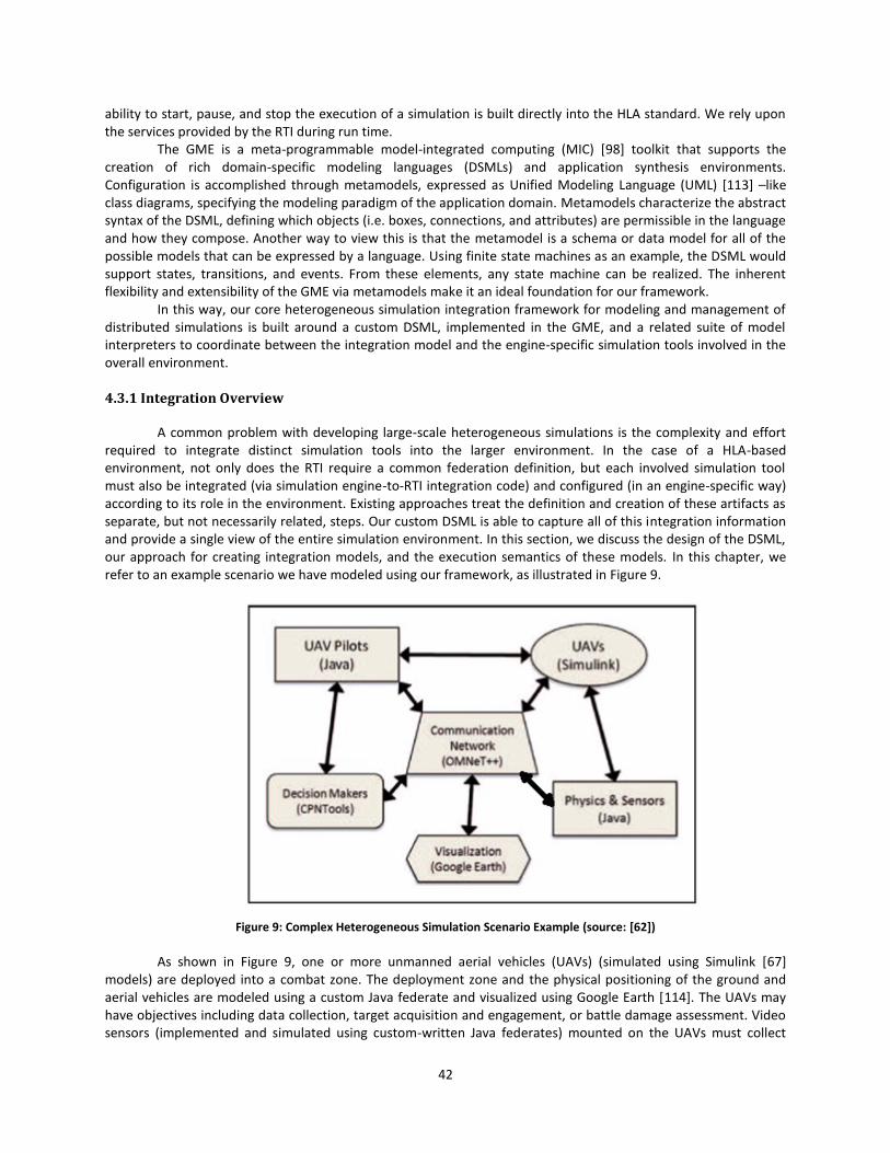
42

ability to start, pause, and stop the execution of a simulation is built directly into the HLA standard. We rely upon the services provided by the RTI during run time.

The GME is a meta-programmable model-integrated computing (MIC) [98] toolkit that supports the creation of rich domain-specific modeling languages (DSMLs) and application synthesis environments. Configuration is accomplished through metamodels, expressed as Unified Modeling Language (UML) [113] –like class diagrams, specifying the modeling paradigm of the application domain. Metamodels characterize the abstract syntax of the DSML, defining which objects (i.e. boxes, connections, and attributes) are permissible in the language and how they compose. Another way to view this is that the metamodel is a schema or data model for all of the possible models that can be expressed by a language. Using finite state machines as an example, the DSML would support states, transitions, and events. From these elements, any state machine can be realized. The inherent flexibility and extensibility of the GME via metamodels make it an ideal foundation for our framework.

In this way, our core heterogeneous simulation integration framework for modeling and management of distributed simulations is built around a custom DSML, implemented in the GME, and a related suite of model interpreters to coordinate between the integration model and the engine-specific simulation tools involved in the overall environment.

4.3.1 Integration Overview

A common problem with developing large-scale heterogeneous simulations is the complexity and effort required to integrate distinct simulation tools into the larger environment. In the case of a HLA-based environment, not only does the RTI require a common federation definition, but each involved simulation tool must also be integrated (via simulation engine-to-RTI integration code) and configured (in an engine-specific way) according to its role in the environment. Existing approaches treat the definition and creation of these artifacts as separate, but not necessarily related, steps. Our custom DSML is able to capture all of this integration information and provide a single view of the entire simulation environment. In this section, we discuss the design of the DSML, our approach for creating integration models, and the execution semantics of these models. In this chapter, we refer to an example scenario we have modeled using our framework, as illustrated in Figure 9.

Figure 9: Complex Heterogeneous Simulation Scenario Example (source: [62])

As shown in Figure 9, one or more unmanned aerial vehicles (UAVs) (simulated using Simulink [67]

models) are deployed into a combat zone. The deployment zone and the physical positioning of the ground and aerial vehicles are modeled using a custom Java federate and visualized using Google Earth [114]. The UAVs may have objectives including data collection, target acquisition and engagement, or battle damage assessment. Video sensors (implemented and simulated using custom-written Java federates) mounted on the UAVs must collect

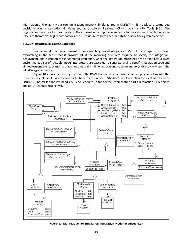
43

information and relay it via a communications network (implemented in OMNeT++ [68]) back to a centralized decision-making organization (implemented as a colored Petri-net (CPN) model in CPN Tools [66]). The organization must react appropriately to the information and provide guidance to the vehicles. In addition, some UAVs are themselves highly autonomous and must utilize collected sensor data to pursue their given objectives.

4.3.2 Integration Modeling Language

Fundamental to our environment is the overarching model integration DSML. This language is considered overarching in the sense that it provides all of the modeling primitives required to specify the integration, deployment, and execution of the federated simulation. Once the integration model has been defined for a given environment, a set of reusable model interpreters are executed to generate engine-specific integration code and all deployment and execution artifacts automatically. All generation and deployment steps directly rely upon the initial integration model.

Figure 10 shows the primary portion of the DSML that defines the universe of composition elements. The three primary elements in a federation (defined by the model FOMSheet) are Interaction (on right-hand side of Figure 10), Object (on the left-hand side), and Federate (in the center), representing a HLA-interaction, HLA-object, and a HLA-federate respectively.

Figure 10: Meta-Model for Simulation Integration Models (source: [62])

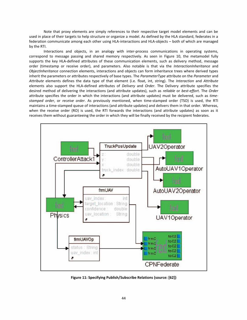
44

Note that proxy elements are simply references to their respective target model elements and can be used in place of their targets to help structure or organize a model. As defined by the HLA standard, federates in a federation communicate among each other using HLA-interactions and HLA-objects – both of which are managed by the RTI.

Interactions and objects, in an analogy with inter-process communications in operating systems, correspond to message passing and shared memory respectively. As seen in Figure 10, the metamodel fully supports the key HLA-defined attributes of these communication elements, such as delivery method, message order (timestamp or receive order), and parameters. Also notable is that via the InteractionInheritance and ObjectInheritance connection elements, interactions and objects can form inheritance trees where derived types inherit the parameters or attributes respectively of base types. The ParameterType attribute on the Parameter and Attribute elements defines the data type of that element (i.e. float, int, string). The Interaction and Attribute elements also support the HLA-defined attributes of Delivery and Order. The Delivery attribute specifies the desired method of delivering the interactions (and attribute updates), such as reliable or best-effort. The Order attribute specifies the order in which the interactions (and attribute updates) must be delivered, such as time-stamped order, or receive order. As previously mentioned, when time-stamped order (TSO) is used, the RTI maintains a time-stamped queue of interactions (and attribute updates) and delivers them in that order. Whereas, when the receive order (RO) is used, the RTI forwards the interactions (and attribute updates) as soon as it receives them without guaranteeing the order in which they will be finally received by the recipient federates.

Figure 11: Specifying Publish/Subscribe Relations (source: [62])

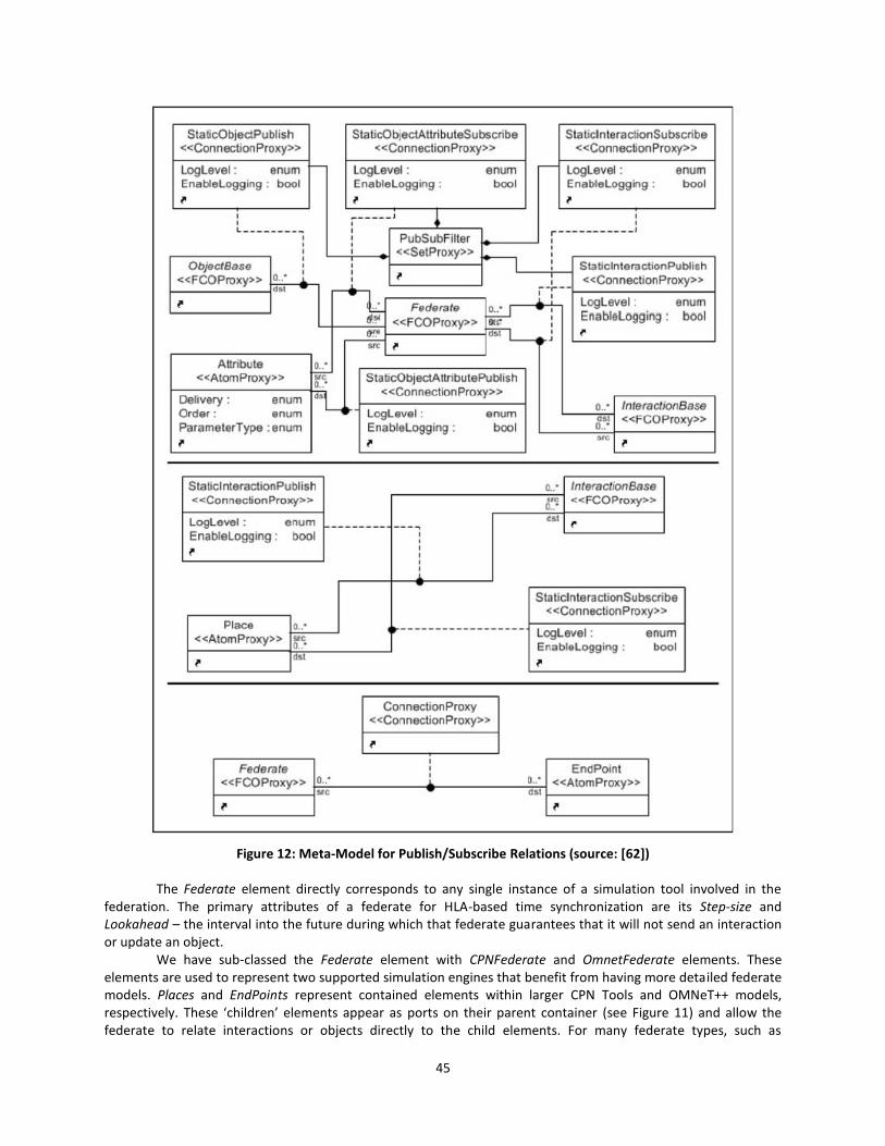
45

Figure 12: Meta-Model for Publish/Subscribe Relations (source: [62])

The Federate element directly corresponds to any single instance of a simulation tool involved in the

federation. The primary attributes of a federate for HLA-based time synchronization are its Step-size and Lookahead – the interval into the future during which that federate guarantees that it will not send an interaction or update an object.

We have sub-classed the Federate element with CPNFederate and OmnetFederate elements. These elements are used to represent two supported simulation engines that benefit from having more detailed federate models. Places and EndPoints represent contained elements within larger CPN Tools and OMNeT++ models, respectively. These ‘children’ elements appear as ports on their parent container (see Figure 11) and allow the federate to relate interactions or objects directly to the child elements. For many federate types, such as

46

Matlab/Simulink or Java/C++, children elements do not have a semantic equivalent, and as such do not need specific support in the metamodel.

Lastly, the attributes of the FOMSheet element capture the names and locations for configuration code that enables the integration of supported simulation engines. We will describe this capability in detail in section 4.4. Collectively, these language elements are required to define the relationships between all federate types. Developing an actual integration model using these special simulation elements is discussed in the subsequent section.

Figure 12 shows additional portions of the DSML. The top portion of the figure shows the language elements necessary to model federates publishing and subscribing interactions, objects, and attributes. A Federate (bottom center of the top portion) can be related to an interaction (inherited via the InteractionBase element – bottom right). Two relationships are possible, publish (via a StaticInteractionPublish connection – middle right) or subscribe (via a StaticInteractionSubscribe connection – top right). Similar relationships exist between objects (via the ObjectBase element) and federates. Since the HLA standard allows federates to subscribe to individual object attributes, the Attribute element supports the subscribe connection to federates. The PubSubFilter element provides a simple means to organize publish-and-subscribe relationships.

The lower two portions of Figure 12 are extensions specific to the integration of CPN Tools and OMNeT++ engines. The middle portion of the model captures publish-and-subscribe links with Place elements. Similarly, the model at the bottom of the figure captures the connection with special-purpose EndPoint elements for the integration of OMNeT++ federates.

This language, and its set of modeling elements, is very closely related to the HLA standard so that it could be easily extended for future extensions to other RTIs in addition to the one currently supported (viz. Portico RTI [21]). With these elements, a designer is able to specify the integration model of the entire federation and its constituent simulation engines. Federates define the details of the engine-specific models that are involved, and their relationships are captured via publishing and subscribing to various interactions and objects. We have further extended the language to include primitives for specifying deployment and execution. These extensions are discussed in section 4.5.

4.3.3 Integration Modeling

The semantic relationship between federates can be defined primarily using two main aspects: the data representation and the data flow. These are common elements of most simulation modeling paradigms, and we have adopted these as the key concepts of our integration models. An integration model describes both data representation and data flow elements, and, in some cases, includes special elements as the placeholders for concepts specific to particular simulation engines.

Data representation models consist of interaction and object models. Interactions are stateless, and can have parameters, while objects have states, which are represented as a set of attributes. Both interactions and objects are permitted to have inheritance hierarchies. These data representation models directly map to the HLA federation object model (FOM).

Figure 13 shows two data representation models from our example: an interaction class-inheritance tree on the top (elements not shaded), and an object class-inheritance tree on the bottom (elements shaded). All interactions must initially inherit from the InteractionRoot element; likewise, all objects must inherit from the ObjectRoot element. While root inheritance is mandated in the HLA standard, we have directly incorporated this concept into the DSML to both clarify the visual representation and to simplify the interpretation of the model tree. Deriving elements via inheritance is an intuitive approach readily understood by modelers.

Once the data representation models are created, the modeler must define publish–subscribe data flow relations with federates. This is accomplished by connecting federates to interactions or object attributes with directional links. Federates publish and subscribe to any set of interactions or objects, dictated solely by the desired operational semantics. Federates can also publish or subscribe to entire data elements or to a subset of their attributes. In Figure 11, we show a simple data flow from our example specifying the publish-and-subscribe relationships between federates (elements shaded) and interactions (elements not shaded).

Integrating engine-specific models together in the central modeling environment is simply a matter of connecting federates to those interactions and objects with which they have publish or subscribe relationships. This greatly simplifies the designer’s job, since they no longer need to directly incorporate engine-specific

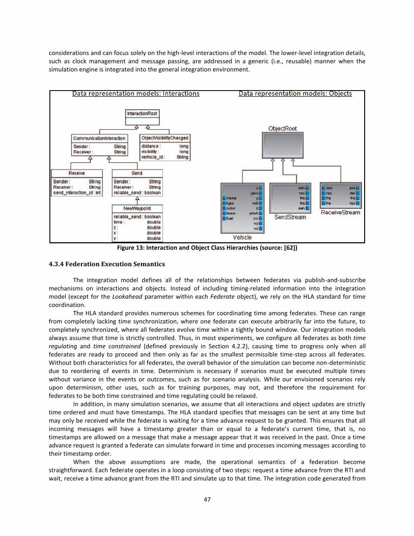
47

considerations and can focus solely on the high-level interactions of the model. The lower-level integration details, such as clock management and message passing, are addressed in a generic (i.e., reusable) manner when the simulation engine is integrated into the general integration environment.

Figure 13: Interaction and Object Class Hierarchies (source: [62])

4.3.4 Federation Execution Semantics

The integration model defines all of the relationships between federates via publish-and-subscribe mechanisms on interactions and objects. Instead of including timing-related information into the integration model (except for the Lookahead parameter within each Federate object), we rely on the HLA standard for time coordination.

The HLA standard provides numerous schemes for coordinating time among federates. These can range from completely lacking time synchronization, where one federate can execute arbitrarily far into the future, to completely synchronized, where all federates evolve time within a tightly bound window. Our integration models always assume that time is strictly controlled. Thus, in most experiments, we configure all federates as both time regulating and time constrained (defined previously in Section 4.2.2), causing time to progress only when all federates are ready to proceed and then only as far as the smallest permissible time-step across all federates. Without both characteristics for all federates, the overall behavior of the simulation can become non-deterministic due to reordering of events in time. Determinism is necessary if scenarios must be executed multiple times without variance in the events or outcomes, such as for scenario analysis. While our envisioned scenarios rely upon determinism, other uses, such as for training purposes, may not, and therefore the requirement for federates to be both time constrained and time regulating could be relaxed.

In addition, in many simulation scenarios, we assume that all interactions and object updates are strictly time ordered and must have timestamps. The HLA standard specifies that messages can be sent at any time but may only be received while the federate is waiting for a time advance request to be granted. This ensures that all incoming messages will have a timestamp greater than or equal to a federate’s current time, that is, no timestamps are allowed on a message that make a message appear that it was received in the past. Once a time advance request is granted a federate can simulate forward in time and processes incoming messages according to their timestamp order.

When the above assumptions are made, the operational semantics of a federation become straightforward. Each federate operates in a loop consisting of two steps: request a time advance from the RTI and wait, receive a time advance grant from the RTI and simulate up to that time. The integration code generated from

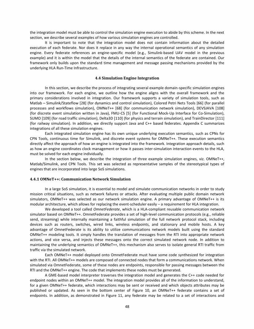
48

the integration model must be able to control the simulation engine execution to abide by this scheme. In the next section, we describe several examples of how various simulation engines are controlled.

It is important to note that the integration model does not contain information about the detailed execution of each federate. Nor does it replace in any way the internal operational semantics of any simulation engine. Every federate references an engine-specific model (e.g., Simulink-based UAV model in the previous example) and it is within the model that the details of the internal semantics of the federate are contained. Our framework only builds upon the standard time management and message passing mechanisms provided by the underlying HLA Run-Time Infrastructure.

4.4 Simulation Engine Integration

In this section, we describe the process of integrating several example domain-specific simulation engines into our framework. For each engine, we outline how the engine aligns with the overall framework and the primary considerations involved in integration. Our framework supports a variety of simulation tools, such as Matlab – Simulink/Stateflow [28] (for dynamics and control simulation), Colored Petri Nets Tools [66] (for parallel processes and workflows simulation), OMNeT++ [68] (for communication network simulation), DEVSJAVA [108] (for discrete event simulation written in Java), FMU-CS [5] (for Functional Mock-Up Interface for Co-Simulation), SUMO [109] (for road traffic simulation), Delta3D [110] (for physics and terrain simulation), and TrainDirector [111] (for railway simulation). In addition, we directly support Java and C++ based federates. Appendix C summarizes integrations of all these simulation engines.

Each integrated simulation engine has its own unique underlying execution semantics, such as CPNs for CPN Tools, continuous time for Simulink, and discrete event systems for OMNeT++. These execution semantics directly affect the approach of how an engine is integrated into the framework. Integration approach details, such as how an engine coordinates clock management or how it passes inter-simulation interaction events to the HLA, must be solved for each engine individually.

In the section below, we describe the integration of three example simulation engines, viz. OMNeT++, Matlab/Simulink, and CPN Tools. This set was selected as representative samples of the stereotypical types of engines that are incorporated into large SoS simulations.

4.4.1 OMNeT++: Communication Network Simulation

In a large SoS simulation, it is essential to model and simulate communication networks in order to study mission critical situations, such as network failures or attacks. After evaluating multiple public domain network simulators, OMNeT++ was selected as our network simulation engine. A primary advantage of OMNeT++ is its modular architecture, which allows for replacing the event-scheduler easily – a requirement for HLA integration.

We developed a tool called OmnetFederate, which is a HLA-compliant reusable communication network simulator based on OMNeT++. OmnetFederate provides a set of high-level communication protocols (e.g., reliable send, streaming) while internally maintaining a faithful simulation of the full network protocol stack, including devices such as routers, switches, wired links, wireless endpoints, and stationary and mobile hosts. A key advantage of OmnetFederate is its ability to utilize communications network models built using the standard OMNeT++ modeling tools. It simply handles the translation of messages from the RTI into appropriate network actions, and vice versa, and injects these messages onto the correct simulated network node. In addition to maintaining the underlying semantics of OMNeT++, this mechanism also serves to isolate general RTI traffic from traffic via the simulated network.

Each OMNeT++ model deployed onto OmnetFederate must have some code synthesized for integration with the RTI. All OMNeT++ models are composed of connected nodes that form a communications network. When simulated via OmnetFederate, some of these nodes are endpoints, responsible for passing messages between the RTI and the OMNeT++ engine. The code that implements these nodes must be generated.

A GME-based model interpreter traverses the integration model and generates the C++ code needed for endpoint nodes within an OMNeT++ model. The integration model provides all of the information to understand, for a given OMNeT++ federate, which interactions may be sent or received and which objects attributes may be published or updated. As seen in the bottom center of Figure 10, an OMNeT++ federate contains a set of endpoints. In addition, as demonstrated in Figure 11, any federate may be related to a set of interactions and

49

objects. The interpreter understands these relationships and synthesizes code for each endpoint in an OMNeT++ federate. The generated code builds upon the OMNeT++ API and compiled directly into the model-independent OmnetFederate tool.

Figure 14: OMNeT++ Scheduler Function (pseudo code)

In addition to inter-federate communication, evolution of the OMNeT++ internal simulation clock must

also be synchronized with the RTI. OmnetFederate includes a reusable class that extends the basic OMNeT++ scheduler. Figure 14 shows the key scheduler function that implements RTI time synchronization. The function is called by OMNeT++ to determine the next event, originated either internally or externally. If the timestamp on the next message places it outside of the window of time granted by the RTI, then a time advance is requested using rti->advanceTime().

An internal dispatch mechanism routes all RTI interactions to the appropriate OMNeT++ protocol module, which interprets them and can schedule new internal OMNeT++ messages. A similar mechanism interprets and routes OMNeT++ messages bound for external dispatch into the RTI. Using these mechanisms, both the evolution of time and message passing within an OMNeT++ federate is tightly coordinated via the RTI with the federation.

4.4.2 Matlab/Simulink: Dynamics and Control Simulation

Matlab/Simulink [67] is a widely used simulation environment for dynamic and embedded systems, such as communications, controls, and signal processing. It is a visual language, which uses a set of pre-built block libraries for designing and controlling the simulation.

Integration of the Simulink simulation engine is similar to that of the OMNeT++ engine in that all of the engine-specific integration code is generated based on the overarching integration model. The GME-based model interpreter generates code that, in conjunction with several generic classes, is used to integrate any Simulink model directly with a SoS federation. The generic classes are completely reusable Java code and provide all of the fundamental RTI integration requirements: providing interfaces for converting between Simulink types and RTI types, encapsulating interfacing with the RTI for initializing the federate, synchronizing the Simulink engine’s simulation clock, and managing any publish-and-subscribe relationships with other federates. The generated Java and Simulink files for the engine integration depend on this reusable code.

Within any given Simulink model, the user must insert an S-function block (a visual block that calls some textual code, specified in an ‘.m’ file, for execution) for each interaction or object to which the model either publishes or subscribes. It is via these blocks that the Simulink engine interacts with the remainder of the federation. The modeler must specify whether the block either publishes or subscribes an interaction or object. This is done by instantiating the corresponding sender or receiver S-function from those that were generated from the integration model. The modeler must also tell the S-function block which interaction or object it should call. This is done by encoding the name of the interaction or object as a parameter to the block. The naming convention of the. m files and of the parameters is standardized and easily derived from the simulation’s data model. Once the S-function blocks have been incorporated and their values set, no further manual steps are typically necessary to prepare the model to be integrated. Some effort may have to be spent to order the signals entering and exiting the S-function blocks properly so that they correspond to the attribute ordering of the corresponding RTI interaction.

50

The key mechanism for synchronizing the clock progression of the Simulink model with that of the RTI is the basic time-progression model for S-function blocks. During its execution, the Simulink engine consults each block in a model about when it can generate an output. With all S-function blocks, code must be supplied, via an implementation of the mdlGetTimeOfNextVarHit() method, to respond to this request from the engine. Typically, this implementation is supplied by the developer (a general Simulink requirement), but, in our case, we generate an implementation from the integration models. For our integration, the synthesized integration code in an S-function block uses this method to synchronize the model with the RTI and allow simulation time within Simulink to progress only when the RTI allows it to proceed. Until the RTI allows federation time to progress, we do not return from the method call within the S-function block, thus not allowing the Simulink engine to progress. We keep the Simulink engine step-size small enough to minimize any event timing errors due to the passing of input and output events between the Simulink model and the HLA. For incoming events, the integration code uses a polling scheme at every time-step to check if the federate has received an input from the remainder of the federation.

Our experience shows that very small step-sizes in any Simulink model can lead to a significant slowdown in simulation speed. In the context of large SoS simulations, possible performance penalties due to having small step-sizes must be weighed against minimizing timing errors due to overly large time-steps. After thorough evaluation, we found that the performance penalty could be reduced to negligible in comparison to the basic lock-stepped simulation we use for synchronizing federates.

4.4.3 CPN Tools: Parallel Processes and Workflows Simulation

In large SoS simulations, it is often needed to evaluate human workflows and the response of decision makers to the evolving situation. In our framework, we use CPN Tools simulator for modeling and simulating human workflows and decision-making processes. We developed methods to integrate CPN models using an augmented version of its BRITNeY [115] extension. This extension provides a low-level bridge between the native CPN Tools API and Java, which simplified integration with the Portico RTI that is written in Java.

The primary challenge involved in integrating the CPN Tools engine into our framework was correct time synchronization. In order to ensure that the CPN model execution stops at desired times one extra place and a transition, which is set to fire with a pre-defined frequency of 1 kHz, are added into a CPN model. The CPN Tools engine optimistically progresses ahead of the HLA clock, but when needed, it can be rolled back to a desired time. This save and restore functionality might be useful for increasing performance using an optimistically large step-size and lookahead. However, with our experiments, we found that the performance penalty incurred by using the small step-size and lookahead was negligible. Thus, we currently use a step-size of ~1 second and lookahead of ~0.1 seconds for most CPN federates. However, while executing the CPN model via the BRITNeY Java library, the CPN clock internally moves forward one millisecond at a time. While time progresses internal to the CPN simulation, we compare its current time with the time granted by the RTI to the CPN federate. If the CPN cannot proceed in time, it requests the RTI to advance time and waits until it receives a time advance grant. While the small internal time-step of CPN federates has the potential to generate significant HLA communications (if there was an interaction every time-step for example), our experience has shown that typical CPN models do not need to interact with the HLA every time-step and thus do not incur a significant overhead.

As illustrated in Figure 15, CPN models are imported into an integration model via an automated model interpreter. Upon importing a CPN model, a CPNFederate element is created within the integration model and the CPN places become corresponding ports on this federate. The ports on this element can then be connected to either interactions or objects to specify inputs and outputs for the CPN model, as discussed in section 4.3.2. This graphical step is the only integration effort necessary for CPN models. All of the engine-specific code to communicate via the RTI and to synchronize the CPN federate with the rest of the federation is generated from the GME integration model.

A custom GME output interpreter generates an extensible markup language (XML) file that describes all of the input–output bindings. The run-time CPN execution engine reads this file and simulates the CPN according to its specification. The set of places to monitor during execution can also be specified. Tokens on these monitored places are shown during run time in a simple Java graphical user interface (GUI) provided by our framework.

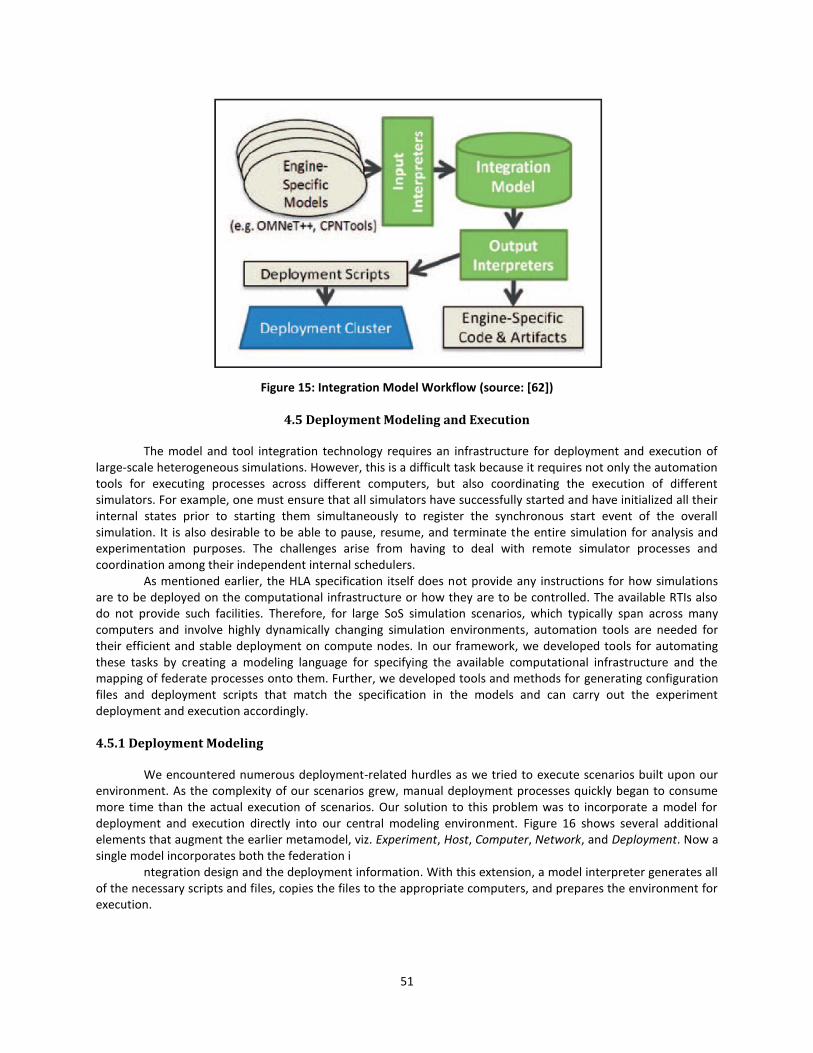
51

Figure 15: Integration Model Workflow (source: [62])

4.5 Deployment Modeling and Execution

The model and tool integration technology requires an infrastructure for deployment and execution of large-scale heterogeneous simulations. However, this is a difficult task because it requires not only the automation tools for executing processes across different computers, but also coordinating the execution of different simulators. For example, one must ensure that all simulators have successfully started and have initialized all their internal states prior to starting them simultaneously to register the synchronous start event of the overall simulation. It is also desirable to be able to pause, resume, and terminate the entire simulation for analysis and experimentation purposes. The challenges arise from having to deal with remote simulator processes and coordination among their independent internal schedulers.

As mentioned earlier, the HLA specification itself does not provide any instructions for how simulations are to be deployed on the computational infrastructure or how they are to be controlled. The available RTIs also do not provide such facilities. Therefore, for large SoS simulation scenarios, which typically span across many computers and involve highly dynamically changing simulation environments, automation tools are needed for their efficient and stable deployment on compute nodes. In our framework, we developed tools for automating these tasks by creating a modeling language for specifying the available computational infrastructure and the mapping of federate processes onto them. Further, we developed tools and methods for generating configuration files and deployment scripts that match the specification in the models and can carry out the experiment deployment and execution accordingly.

4.5.1 Deployment Modeling

We encountered numerous deployment-related hurdles as we tried to execute scenarios built upon our environment. As the complexity of our scenarios grew, manual deployment processes quickly began to consume more time than the actual execution of scenarios. Our solution to this problem was to incorporate a model for deployment and execution directly into our central modeling environment. Figure 16 shows several additional elements that augment the earlier metamodel, viz. Experiment, Host, Computer, Network, and Deployment. Now a single model incorporates both the federation i

ntegration design and the deployment information. With this extension, a model interpreter generates all of the necessary scripts and files, copies the files to the appropriate computers, and prepares the environment for execution.

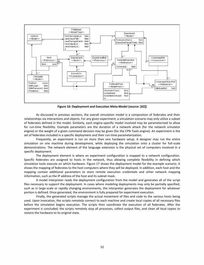
52

Figure 16: Deployment and Execution Meta-Model (source: [62])

As discussed in previous sections, the overall simulation model is a composition of federates and their

relationships via interactions and objects. For any given experiment, a simulation scenario may only utilize a subset of federates defined in the model. Similarly, each engine-specific model involved may be parameterized to allow for run-time flexibility. Example parameters are the duration of a network attack (for the network simulator engine) or the weight of a given command decision may be given (for the CPN Tools engine). An experiment is the set of federates included in a specific deployment and their run-time parameterization.

Frequently, an experiment is run on more than one hardware setup. A designer may run the entire simulation on one machine during development, while deploying the simulation onto a cluster for full-scale demonstrations. The network element of the language extension is the physical set of computers involved in a specific deployment.

The deployment element is where an experiment configuration is mapped to a network configuration. Specific federates are assigned to hosts in the network, thus allowing complete flexibility in defining which simulation tools execute on which hardware. Figure 17 shows the deployment model for the example scenario. It shows the mapping of federates to the host computers where they will be deployed. In addition, each host and the mapping contain additional parameters to store remote execution credentials and other network mapping information, such as the IP address of the host and its subnet mask.

A model interpreter reads the deployment configuration from the model and generates all of the script files necessary to support the deployment. In cases where modeling deployments may only be partially specified, such as in large-scale or rapidly changing environments, the interpreter generates the deployment for whatever portion is defined. Once generated, the environment is fully prepared for experiment execution.

Finally, the generated scripts manage the actual movement of files and code to the various hosts being used. Upon invocation, the scripts remotely connect to each machine and create local copies of all necessary files before the simulation begins execution. The scripts then coordinate the execution of all federates. After the experiment is concluded, the scripts remotely stop all processes, collect output files, and clean all local copies to restore the hardware to its original state.

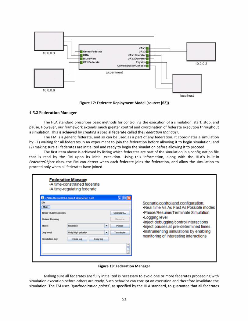
53

Figure 17: Federate Deployment Model (source: [62])

4.5.2 Federation Manager

The HLA standard prescribes basic methods for controlling the execution of a simulation: start, stop, and pause. However, our framework extends much greater control and coordination of federate execution throughout a simulation. This is achieved by creating a special federate called the Federation Manager.

The FM is a generic federate, and so can be used as a part of any federation. It coordinates a simulation by: (1) waiting for all federates in an experiment to join the federation before allowing it to begin simulation; and (2) making sure all federates are initialized and ready to begin the simulation before allowing it to proceed.

The first item above is achieved by listing which federates are part of the simulation in a configuration file that is read by the FM upon its initial execution. Using this information, along with the HLA’s built-in FederateObject class, the FM can detect when each federate joins the federation, and allow the simulation to proceed only when all federates have joined.

Figure 18: Federation Manager

Making sure all federates are fully initialized is necessary to avoid one or more federates proceeding with

simulation execution before others are ready. Such behavior can corrupt an execution and therefore invalidate the simulation. The FM uses ‘synchronization points’, as specified by the HLA standard, to guarantee that all federates

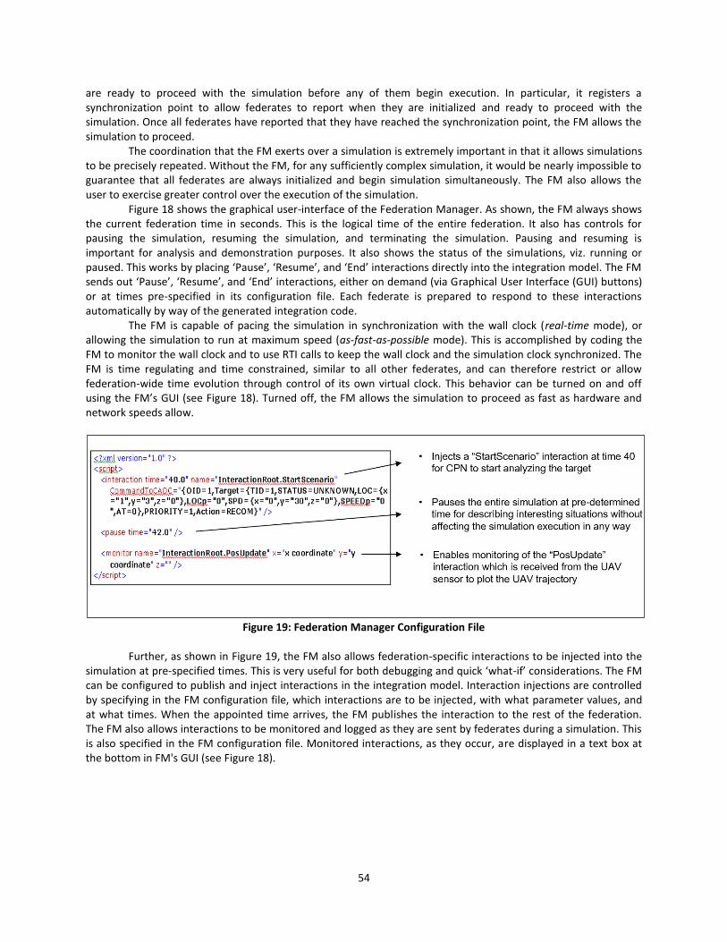
54

are ready to proceed with the simulation before any of them begin execution. In particular, it registers a synchronization point to allow federates to report when they are initialized and ready to proceed with the simulation. Once all federates have reported that they have reached the synchronization point, the FM allows the simulation to proceed.

The coordination that the FM exerts over a simulation is extremely important in that it allows simulations to be precisely repeated. Without the FM, for any sufficiently complex simulation, it would be nearly impossible to guarantee that all federates are always initialized and begin simulation simultaneously. The FM also allows the user to exercise greater control over the execution of the simulation.

Figure 18 shows the graphical user-interface of the Federation Manager. As shown, the FM always shows the current federation time in seconds. This is the logical time of the entire federation. It also has controls for pausing the simulation, resuming the simulation, and terminating the simulation. Pausing and resuming is important for analysis and demonstration purposes. It also shows the status of the simulations, viz. running or paused. This works by placing ‘Pause’, ‘Resume’, and ‘End’ interactions directly into the integration model. The FM sends out ‘Pause’, ‘Resume’, and ‘End’ interactions, either on demand (via Graphical User Interface (GUI) buttons) or at times pre-specified in its configuration file. Each federate is prepared to respond to these interactions automatically by way of the generated integration code.

The FM is capable of pacing the simulation in synchronization with the wall clock (real-time mode), or allowing the simulation to run at maximum speed (as-fast-as-possible mode). This is accomplished by coding the FM to monitor the wall clock and to use RTI calls to keep the wall clock and the simulation clock synchronized. The FM is time regulating and time constrained, similar to all other federates, and can therefore restrict or allow federation-wide time evolution through control of its own virtual clock. This behavior can be turned on and off using the FM’s GUI (see Figure 18). Turned off, the FM allows the simulation to proceed as fast as hardware and network speeds allow.

Figure 19: Federation Manager Configuration File

Further, as shown in Figure 19, the FM also allows federation-specific interactions to be injected into the

simulation at pre-specified times. This is very useful for both debugging and quick ‘what-if’ considerations. The FM can be configured to publish and inject interactions in the integration model. Interaction injections are controlled by specifying in the FM configuration file, which interactions are to be injected, with what parameter values, and at what times. When the appointed time arrives, the FM publishes the interaction to the rest of the federation. The FM also allows interactions to be monitored and logged as they are sent by federates during a simulation. This is also specified in the FM configuration file. Monitored interactions, as they occur, are displayed in a text box at the bottom in FM's GUI (see Figure 18).

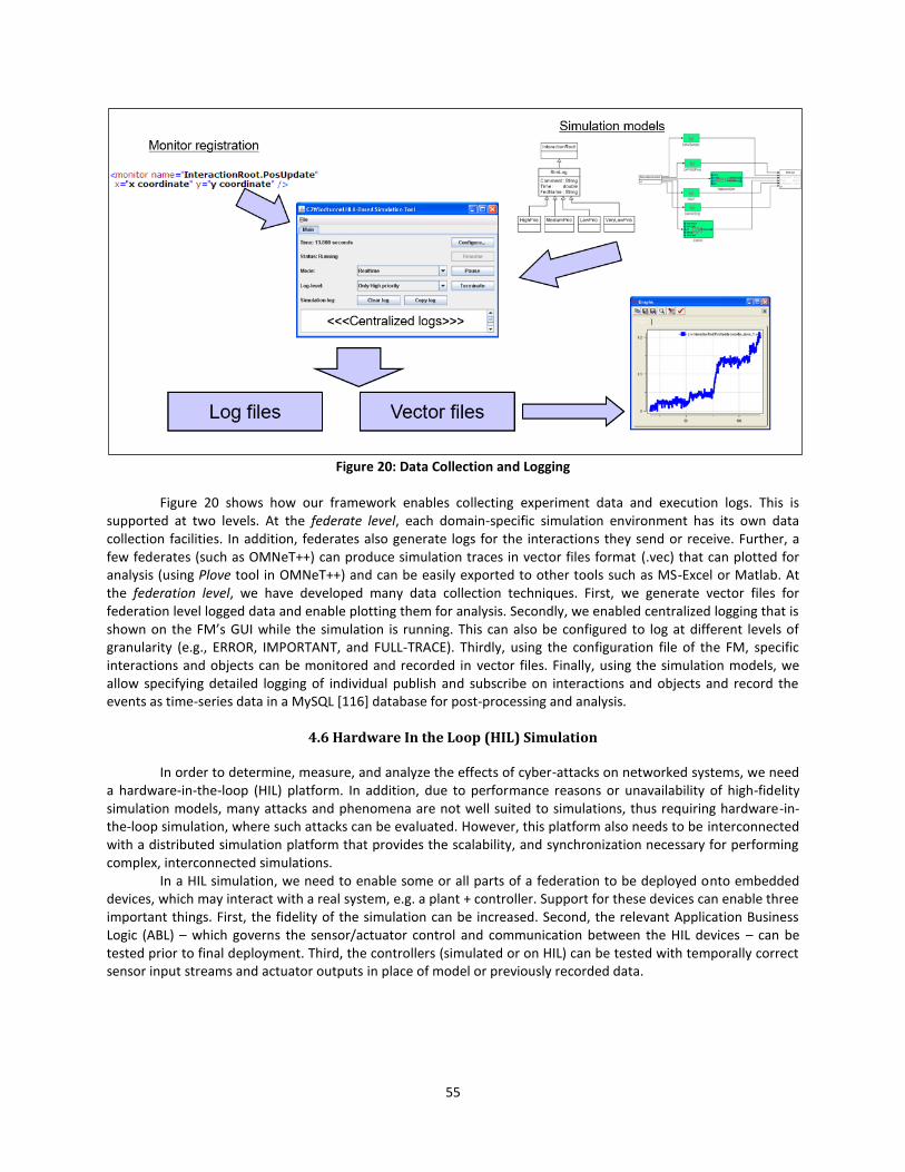
55

Figure 20: Data Collection and Logging

Figure 20 shows how our framework enables collecting experiment data and execution logs. This is

supported at two levels. At the federate level, each domain-specific simulation environment has its own data collection facilities. In addition, federates also generate logs for the interactions they send or receive. Further, a few federates (such as OMNeT++) can produce simulation traces in vector files format (.vec) that can plotted for analysis (using Plove tool in OMNeT++) and can be easily exported to other tools such as MS-Excel or Matlab. At the federation level, we have developed many data collection techniques. First, we generate vector files for federation level logged data and enable plotting them for analysis. Secondly, we enabled centralized logging that is shown on the FM’s GUI while the simulation is running. This can also be configured to log at different levels of granularity (e.g., ERROR, IMPORTANT, and FULL-TRACE). Thirdly, using the configuration file of the FM, specific interactions and objects can be monitored and recorded in vector files. Finally, using the simulation models, we allow specifying detailed logging of individual publish and subscribe on interactions and objects and record the events as time-series data in a MySQL [116] database for post-processing and analysis.

4.6 Hardware In the Loop (HIL) Simulation

In order to determine, measure, and analyze the effects of cyber-attacks on networked systems, we need a hardware-in-the-loop (HIL) platform. In addition, due to performance reasons or unavailability of high-fidelity simulation models, many attacks and phenomena are not well suited to simulations, thus requiring hardware-in-the-loop simulation, where such attacks can be evaluated. However, this platform also needs to be interconnected with a distributed simulation platform that provides the scalability, and synchronization necessary for performing complex, interconnected simulations.

In a HIL simulation, we need to enable some or all parts of a federation to be deployed onto embedded devices, which may interact with a real system, e.g. a plant + controller. Support for these devices can enable three important things. First, the fidelity of the simulation can be increased. Second, the relevant Application Business Logic (ABL) – which governs the sensor/actuator control and communication between the HIL devices – can be tested prior to final deployment. Third, the controllers (simulated or on HIL) can be tested with temporally correct sensor input streams and actuator outputs in place of model or previously recorded data.

56

4.6.1 Fundamental Issues with HIL

For integration of HIL, we need to resolve many fundamental problems, viz. timing issues, networking issues, hardware interactions issues, and software and infrastructure issues.

4.6.1.1 Timing Issues

HIL devices always run in real-time, meaning that their clocks all run asynchronously, and will have different offsets and drift characteristics from each other. These clocks cannot and should not be controlled through HLA, and synchronization of the clocks in the federation (including the clocks on the machines running simulation federates) should be handled by existing and mature clock synchronization service such as NTP. Implicit in the execution of real-time HIL federates according to their synchronized hardware clocks is that these federates are neither time regulating nor time constrained, meaning they are event-driven. Also implicit in the execution semantics is that the simulation federates in the federation must be capable of executing faster than real-time for the relevant input sets and configurations (since execution time of a step of a simulation is heavily input and configuration dependent). Finally, just as simulation federates must translate from federation logical time to local simulation time, so too must the HIL federates translate message timestamps from simulation logical time to an epoch time (i.e. a reference point from which time is measured). This translation of message timestamps must be done in accordance with hardware clock of the computer where the HIL federate runs. Similarly, a reverse translation is needed while generating interactions for the rest of the federation.

4.6.1.2 Networking Issues

Within the realm of the simulated federates communicating using HLA as the interface layer, the network purely serves to pass the interactions from federate to federate (see Figure 21). The timing and capacity properties of the network-links between federates has no effect on the logical execution of the distributed simulation, i.e. in no way does it affect the outcome of the simulation. The simulation is unaffected because federates evolve according to only the logical simulation time which is wholly decoupled from the wall-clock time of any of the interactions. Since the network can only affect the wall-clock timing characteristics of interactions, it cannot affect the data or time of the simulation.

Figure 21: Network Links between HLA Federates and HIL

In contrast, HIL evolves according to the hardware clock (which is directly coupled to the wall-clock). As

such, the timing characteristics, which the network can introduce on the packets, directly affect the HIL execution and evolution.

Figure 22: HIL to HIL Communication

Additionally, HIL may exist as multiple physical devices connected through a real or emulated network

(which itself may exist, for example, as ETH, Wi-Fi, CAN, and I2C). For messages passing between devices on this network (i.e. HIL to HIL), HLA is not used; instead the transport protocol and (de-)marshalling used is the

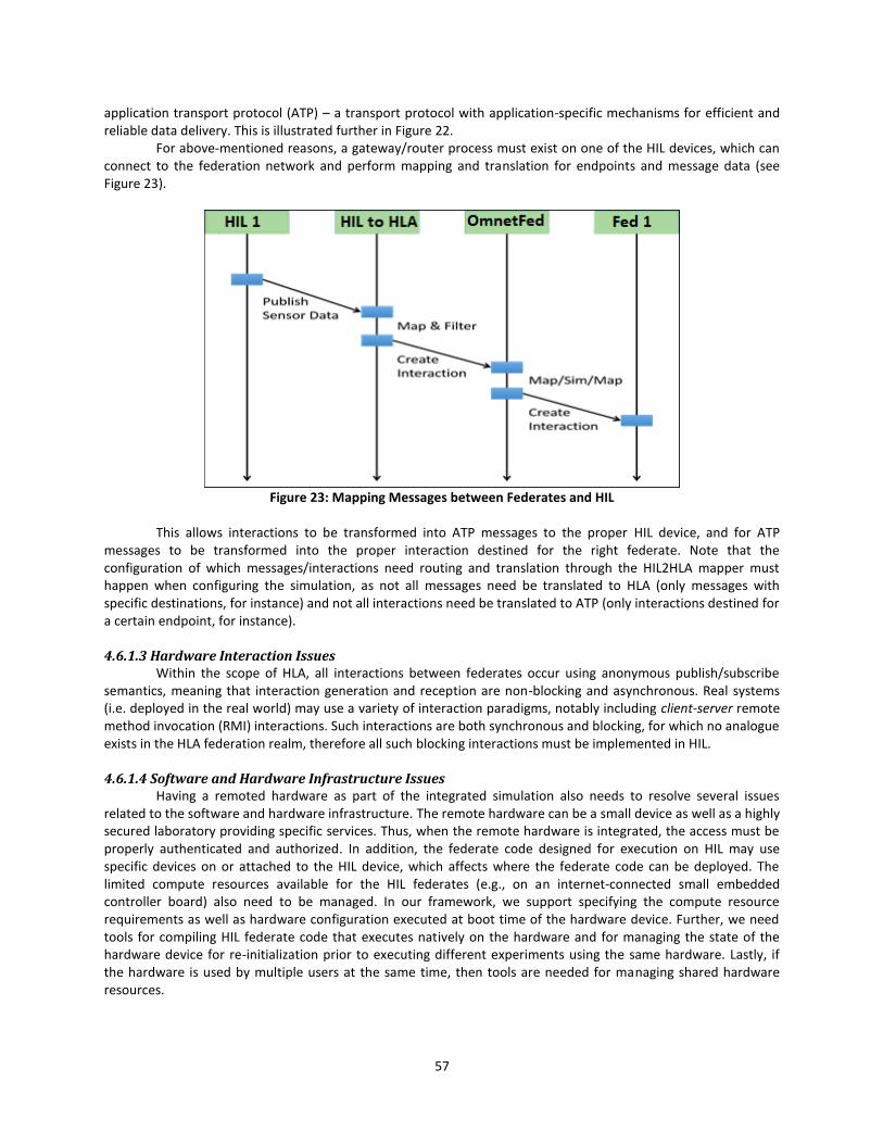
57

application transport protocol (ATP) – a transport protocol with application-specific mechanisms for efficient and reliable data delivery. This is illustrated further in Figure 22.

For above-mentioned reasons, a gateway/router process must exist on one of the HIL devices, which can connect to the federation network and perform mapping and translation for endpoints and message data (see Figure 23).

Figure 23: Mapping Messages between Federates and HIL

This allows interactions to be transformed into ATP messages to the proper HIL device, and for ATP

messages to be transformed into the proper interaction destined for the right federate. Note that the configuration of which messages/interactions need routing and translation through the HIL2HLA mapper must happen when configuring the simulation, as not all messages need be translated to HLA (only messages with specific destinations, for instance) and not all interactions need be translated to ATP (only interactions destined for a certain endpoint, for instance).

4.6.1.3 Hardware Interaction Issues

Within the scope of HLA, all interactions between federates occur using anonymous publish/subscribe semantics, meaning that interaction generation and reception are non-blocking and asynchronous. Real systems (i.e. deployed in the real world) may use a variety of interaction paradigms, notably including client-server remote method invocation (RMI) interactions. Such interactions are both synchronous and blocking, for which no analogue exists in the HLA federation realm, therefore all such blocking interactions must be implemented in HIL.

4.6.1.4 Software and Hardware Infrastructure Issues

Having a remoted hardware as part of the integrated simulation also needs to resolve several issues related to the software and hardware infrastructure. The remote hardware can be a small device as well as a highly secured laboratory providing specific services. Thus, when the remote hardware is integrated, the access must be properly authenticated and authorized. In addition, the federate code designed for execution on HIL may use specific devices on or attached to the HIL device, which affects where the federate code can be deployed. The limited compute resources available for the HIL federates (e.g., on an internet-connected small embedded controller board) also need to be managed. In our framework, we support specifying the compute resource requirements as well as hardware configuration executed at boot time of the hardware device. Further, we need tools for compiling HIL federate code that executes natively on the hardware and for managing the state of the hardware device for re-initialization prior to executing different experiments using the same hardware. Lastly, if the hardware is used by multiple users at the same time, then tools are needed for managing shared hardware resources.

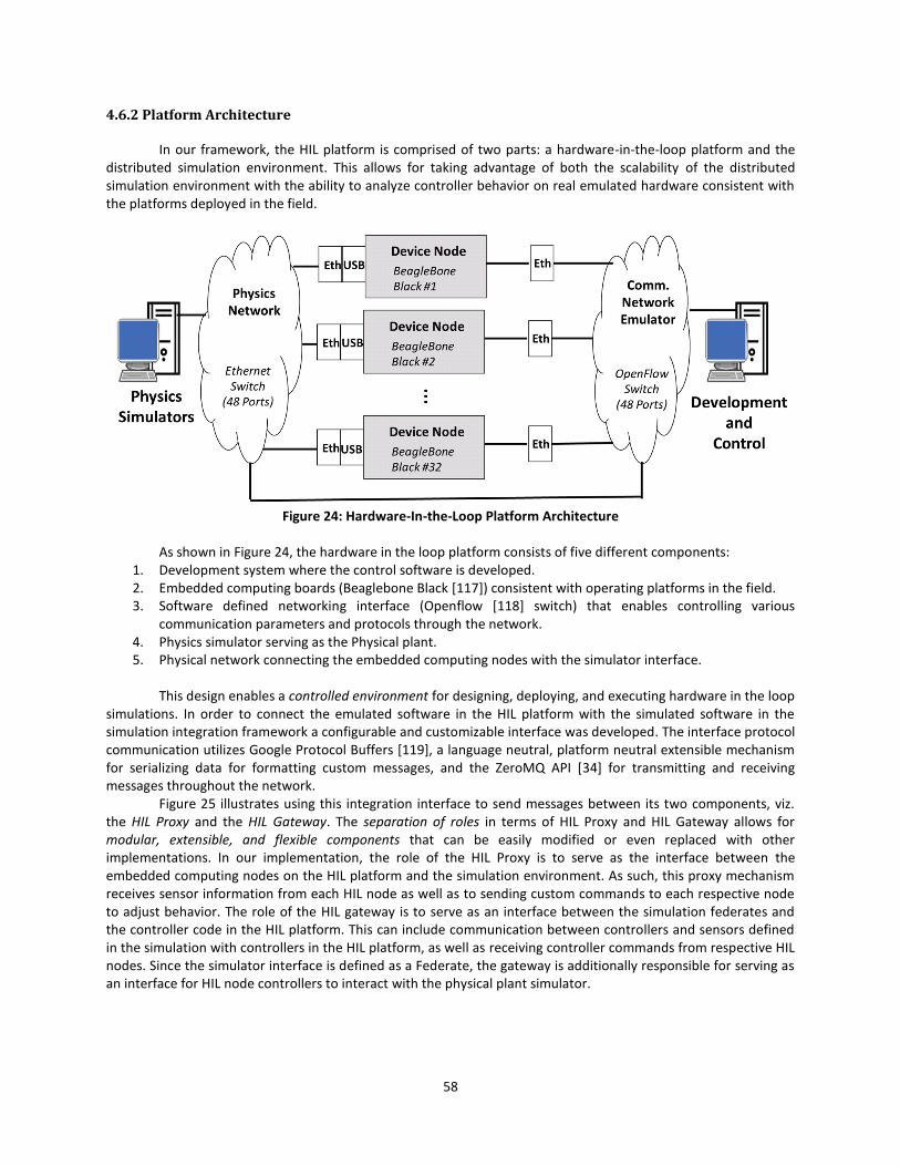
58

4.6.2 Platform Architecture

In our framework, the HIL platform is comprised of two parts: a hardware-in-the-loop platform and the distributed simulation environment. This allows for taking advantage of both the scalability of the distributed simulation environment with the ability to analyze controller behavior on real emulated hardware consistent with the platforms deployed in the field.

Figure 24: Hardware-In-the-Loop Platform Architecture

As shown in Figure 24, the hardware in the loop platform consists of five different components:

1. Development system where the control software is developed. 2. Embedded computing boards (Beaglebone Black [117]) consistent with operating platforms in the field. 3. Software defined networking interface (Openflow [118] switch) that enables controlling various

communication parameters and protocols through the network. 4. Physics simulator serving as the Physical plant. 5. Physical network connecting the embedded computing nodes with the simulator interface.

This design enables a controlled environment for designing, deploying, and executing hardware in the loop

simulations. In order to connect the emulated software in the HIL platform with the simulated software in the simulation integration framework a configurable and customizable interface was developed. The interface protocol communication utilizes Google Protocol Buffers [119], a language neutral, platform neutral extensible mechanism for serializing data for formatting custom messages, and the ZeroMQ API [34] for transmitting and receiving messages throughout the network.

Figure 25 illustrates using this integration interface to send messages between its two components, viz. the HIL Proxy and the HIL Gateway. The separation of roles in terms of HIL Proxy and HIL Gateway allows for modular, extensible, and flexible components that can be easily modified or even replaced with other implementations. In our implementation, the role of the HIL Proxy is to serve as the interface between the embedded computing nodes on the HIL platform and the simulation environment. As such, this proxy mechanism receives sensor information from each HIL node as well as to sending custom commands to each respective node to adjust behavior. The role of the HIL gateway is to serve as an interface between the simulation federates and the controller code in the HIL platform. This can include communication between controllers and sensors defined in the simulation with controllers in the HIL platform, as well as receiving controller commands from respective HIL nodes. Since the simulator interface is defined as a Federate, the gateway is additionally responsible for serving as an interface for HIL node controllers to interact with the physical plant simulator.

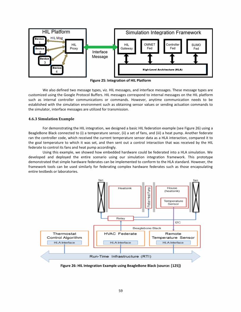
59

Figure 25: Integration of HIL Platform

We also defined two message types, viz. HIL messages, and interface messages. These message types are

customized using the Google Protocol Buffers. HIL messages correspond to internal messages on the HIL platform such as internal controller communications or commands. However, anytime communication needs to be established with the simulation environment such as obtaining sensor values or sending actuation commands to the simulator, interface messages are utilized for transmission.

4.6.3 Simulation Example

For demonstrating the HIL integration, we designed a basic HIL federation example (see Figure 26) using a BeagleBone Black connected to (i) a temperature sensor, (ii) a set of fans, and (iii) a heat pump. Another federate ran the controller code, which received the current temperature sensor data as a HLA interaction, compared it to the goal temperature to which it was set, and then sent out a control interaction that was received by the HIL federate to control its fans and heat pump accordingly.

Using this example, we showed how embedded hardware could be federated into a HLA simulation. We developed and deployed the entire scenario using our simulation integration framework. This prototype demonstrated that simple hardware federates can be implemented to conform to the HLA standard. However, the framework tools can be used similarly for federating complex hardware federates such as those encapsulating entire testbeds or laboratories.

Figure 26: HIL Integration Example using BeagleBone Black (source: [125])

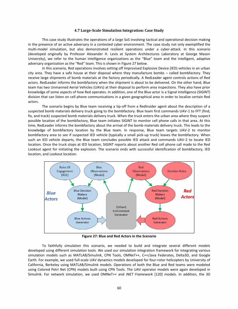
60

4.7 Large-Scale Simulation Integration: Case Study

This case study illustrates the operations of a large SoS involving tactical and operational decision making in the presence of an active adversary in a contested cyber environment. The case study not only exemplified the multi-model simulation, but also demonstrated resilient operations under a cyber-attack. In this scenario (developed originally by Professor Alexander H. Levis at System Architectures Laboratory at George Mason University), we refer to the human intelligence organizations as the “Blue” team and the intelligent, adaptive adversary organization as the “Red” team. This is shown in Figure 27 below.

In this scenario, Red operations involves setting off Improvised Explosive Device (IED) vehicles in an urban city area. They have a safe house at their disposal where they manufacture bombs – called bombfactory. They receive large shipments of bomb materials at the factory periodically. A RedLeader agent controls actions of Red actors. RedLeader informs the bombfactory when the shipment is about to be delivered. On the other hand, Blue team has two Unmanned Aerial Vehicles (UAVs) at their disposal to perform area inspections. They also have prior knowledge of some aspects of how Red operates. In addition, one of the Blue actor is a Signal Intelligence (SIGINT) division that can listen on cell phone communications in a given geographical area in order to localize certain Red actors.

The scenario begins by Blue team receiving a tip-off from a RedInsider agent about the description of a suspected bomb materials delivery truck going to the bombfactory. Blue team first commands UAV-1 to FFT (find, fix, and track) suspected bomb materials delivery truck. When the truck enters the urban area where they suspect possible location of the bombfactory, Blue team initiates SIGINT to monitor cell phone calls in that area. At this time, RedLeader informs the bombfactory about the arrival of the bomb materials delivery truck. This leads to the knowledge of bombfactory location by the Blue team. In response, Blue team targets UAV-2 to monitor bombfactory area to see if suspected IED vehicle (typically a small pick-up truck) leaves the bombfactory. When such an IED vehicle departs, the Blue team concludes possible IED attack and commands UAV-2 to locate IED location. Once the truck stops at IED location, SIGINT reports about another Red cell phone call made to the Red Lookout agent for initiating the explosion. The scenario ends with successful identification of bombfactory, IED location, and Lookout location.

Figure 27: Blue and Red Actors in the Scenario

To faithfully simulation this scenario, we needed to build and integrate several different models

developed using different simulation tools. We used our simulation integration framework for integrating various simulation models such as MATLAB/Simulink, CPN Tools, OMNeT++, C++/Java Federates, Delta3D, and Google Earth. For example, we used full-scale UAV dynamics models developed for four-rotor helicopters by University of California, Berkeley using MATLAB/Simulink models. Operations of both the Blue and Red teams were modeled using Colored Petri Net (CPN) models built using CPN Tools. The UAV operator models were again developed in Simulink. For network simulation, we used OMNeT++ and INET Framework [120] models. In addition, the 3D

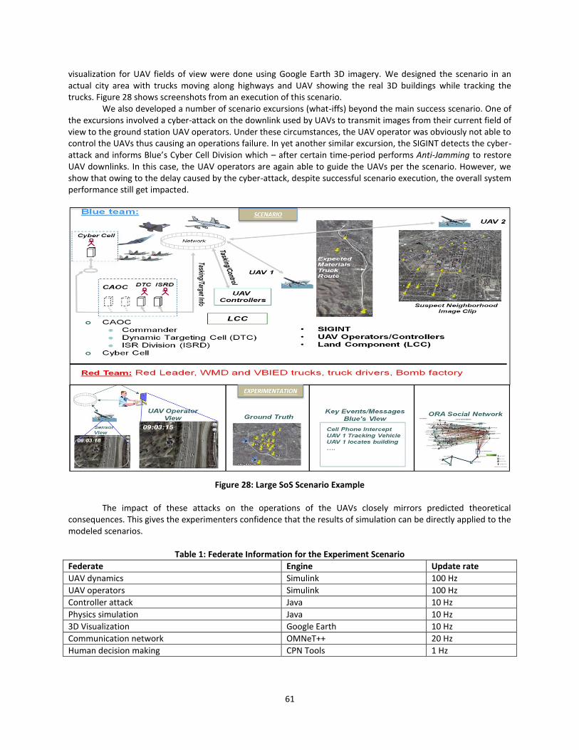
61

visualization for UAV fields of view were done using Google Earth 3D imagery. We designed the scenario in an actual city area with trucks moving along highways and UAV showing the real 3D buildings while tracking the trucks. Figure 28 shows screenshots from an execution of this scenario.

We also developed a number of scenario excursions (what-iffs) beyond the main success scenario. One of the excursions involved a cyber-attack on the downlink used by UAVs to transmit images from their current field of view to the ground station UAV operators. Under these circumstances, the UAV operator was obviously not able to control the UAVs thus causing an operations failure. In yet another similar excursion, the SIGINT detects the cyber-attack and informs Blue’s Cyber Cell Division which – after certain time-period performs Anti-Jamming to restore UAV downlinks. In this case, the UAV operators are again able to guide the UAVs per the scenario. However, we show that owing to the delay caused by the cyber-attack, despite successful scenario execution, the overall system performance still get impacted.

Figure 28: Large SoS Scenario Example

The impact of these attacks on the operations of the UAVs closely mirrors predicted theoretical

consequences. This gives the experimenters confidence that the results of simulation can be directly applied to the modeled scenarios.

Table 1: Federate Information for the Experiment Scenario

Federate Engine Update rate

UAV dynamics Simulink 100 Hz

UAV operators Simulink 100 Hz

Controller attack Java 10 Hz

Physics simulation Java 10 Hz

3D Visualization Google Earth 10 Hz

Communication network OMNeT++ 20 Hz

Human decision making CPN Tools 1 Hz

62

Table 1 captures the engine type and update rate for each of federates involved in our simulation. Our hardware configuration used during demonstrations consists of six dual-core 3.0 GHz-class machines networked via a dedicated 100 Mb/s switch all with nVidia GTX 280 graphics cards. In a typical deployment, each machine had between one and three federates running on it. Despite highly complex engine-specific models, we have not experienced any significant performance bottlenecks during simulations lasting an average of about 30 minutes. If our scenarios are deployed entirely onto one of our typical development machines (a clone of those in our demonstration cluster) performance is acceptable but noticeably slower – took about 90-150 minutes depending on how many visualization federates were used.

Using our framework, new scenarios can be created within a few weeks or even days. For example, it took us less than three weeks to create a new scenario as compared to anecdotal evidence that, prior to our framework, developing individual scenarios in practice could take between one and two years to develop. Notice, however, that our scenario did not require the integration of any new simulation engines as all the needed simulation engines were apriori supported by the framework.

4.8 Levels of Users of the Integration Framework

A distributed simulation framework is developed and used by three different levels of users (see Appendix D). At the top are the Experiment Designers and Analysts who perform studies and evaluations by designing experimental scenarios on a configured system and running experiments using those scenarios. The second level of users include the System Modelers and Integrators who have the knowledge of system-of-system architecture of the overall system that is being simulated in an integrated manner. These users can create models and artifacts needed for new studies. Lastly, the third level of users are the Infrastructure Developers and Maintainers who have deep technical knowledge to incorporate new simulation tools in the infrastructure, to build and enable parameters for the individual models and experiments, as well as to develop and maintain the build systems and necessary tooling in the infrastructure.

As the framework is developed and shared among these different levels of users, a well-defined approach must be used to develop, test, and make available the framework features and tools among its users. Our use of: (1) metamodeling, (2) model-based integration of distributed simulations, and (3) automated deployment of experiments, allowed us to create a framework that can be customized/extended by all of the three levels of users.

4.9 Summary

Integration of large SoS simulations composed of numerous heterogeneous engines is a challenging problem. These systems are complex, very large, highly heterogeneous, and very difficult to analyze comprehensively. Each simulation engine may have its own operational semantics and requires integration at not only the engine level, but also at the engine-specific model level. For effective evaluation of large SoSs, we need to perform integrated simulations of all its systems in a logically and temporally coherent manner.

Use of models throughout simulation engines, opens the door to the use of model-integrated methodologies for defining integration among these tools. In this chapter, we described a model-based simulation integration and experimentation framework that enables researchers to integrate and evaluate large SoS simulations, and assess, evaluate, and validate their algorithms in realistic scenarios. In this framework, it is possible to integrate domain-specific models rapidly from diverse simulation engines and to generate all of the needed configuration and integration code dynamically. The environment also provides automated facilities to manage the deployment and execution of the simulation itself. Together these tools greatly reduce the time required to design, modify, and test large SoS simulation scenarios.

63

CHAPTER 5. MAPPING METHODS FOR LEGACY COMPONENT INTEGRATION

5.1 Introduction

One of the core functionality of our framework is to support easier integration of a variety of simulation tools. The aim is to be able to support the tools without user having to write code for encoding/decoding message in formats that other simulation tools understand.

A key assumption we made so far is that all federates can agree to use a common data model for exchanging data among themselves. However, in some SoS simulations, this may not be possible for several reasons. First, in order to integrate a simulation tool, it must have open and documented APIs for interfacing with it for inputs and outputs and for controlling its execution for time synchronization with other simulation tools. In some cases (e.g., classified or proprietary simulation tools), this is not the case. Consequently, it is not possible to use an externally defined common data model. Therefore, this usually requires a translation between commonly agreed upon data model and the format of the messages that the simulation tool can understand and generate. Secondly, even if the simulation tool has an interface API (and even if the tool is completely open-source), a lot of tedious customization might be necessary for integrating the simulation tool in the distributed simulation. For example, the simulation tool may allow some level of configuration of its input and output ports, but may require substantial source code changes to write custom business logic of mapping (and aggregating/ disaggregating) messages in the common data model to its internal message- (or even file-) formats, and, possibly, to customize its defined APIs. Furthermore, modifying simulation tool’s sources/APIs not only requires recompiling them, but also requires source-code modification every time the integration model (containing the common data model) is updated. Thus, the cost of updating, testing, and debugging the modified simulation code could be substantial.

For these reasons, it is desirable to separate the translation logic (called mappings) from the core simulation source-code. In this case, we need automated mapping methods that can enable the use of its proprietary HLA FOM (Federation Object Model) [20] models and automated message encoding/decoding into FOM used by other simulator tools or a particular scenario/demo model. Therefore, we argue that:

“The translation logic should not be mixed in the core application logic in the simulation tools because it is more time-consuming to write and debug the modified main simulation code, the approach is inflexible for changes/reuse in different applications domains and models, it cannot support integration with multiple simulation tools used in the SoS, and it is an error-prone approach that is hard to maintain.”

The above observation is true for both when the translation code resides adjacent to the core simulation

code in each of the simulation tools or resides for some or all simulation tools in a separate intermediary federate (called a mapper). Note that this is closely related to the techniques for translating/matching database schema from one format to the other, which may include pattern-based matching at different hierarchical levels of schema concepts as well as language- and constraint-based matchers [94]. However, in a mapper, the translation could also depend on the content of the messages mapped. Further, database schema translation usually supports only one-to-one, one-to-many, and many-to-one translations, whereas in a mapper many-to-many translations may also be needed.

Figure 29XX illustrates how mappers can be used in order to support automated message translation among different simulation tools. As shown, two simulation engines, viz. ‘X’ and ‘Y’, are being used in a sample federation. The simulation engine ‘X’ uses FOM/SOM definition ‘A’ and the simulation engine ‘Y’ uses the FOM definition ‘B’. As such, the FOM definitions ‘A’ and ‘B’ contain quite different HLA-interactions (i.e. message types). In order for the two simulation engines to understand the interactions of one another, there must be a way to translate the interactions according to their own FOM/SOM definitions. It is important to note that the mapper translates messages, but does not translate among protocols (i.e., it only translates between published and subscribed messages – this fits well to the HLA philosophy).

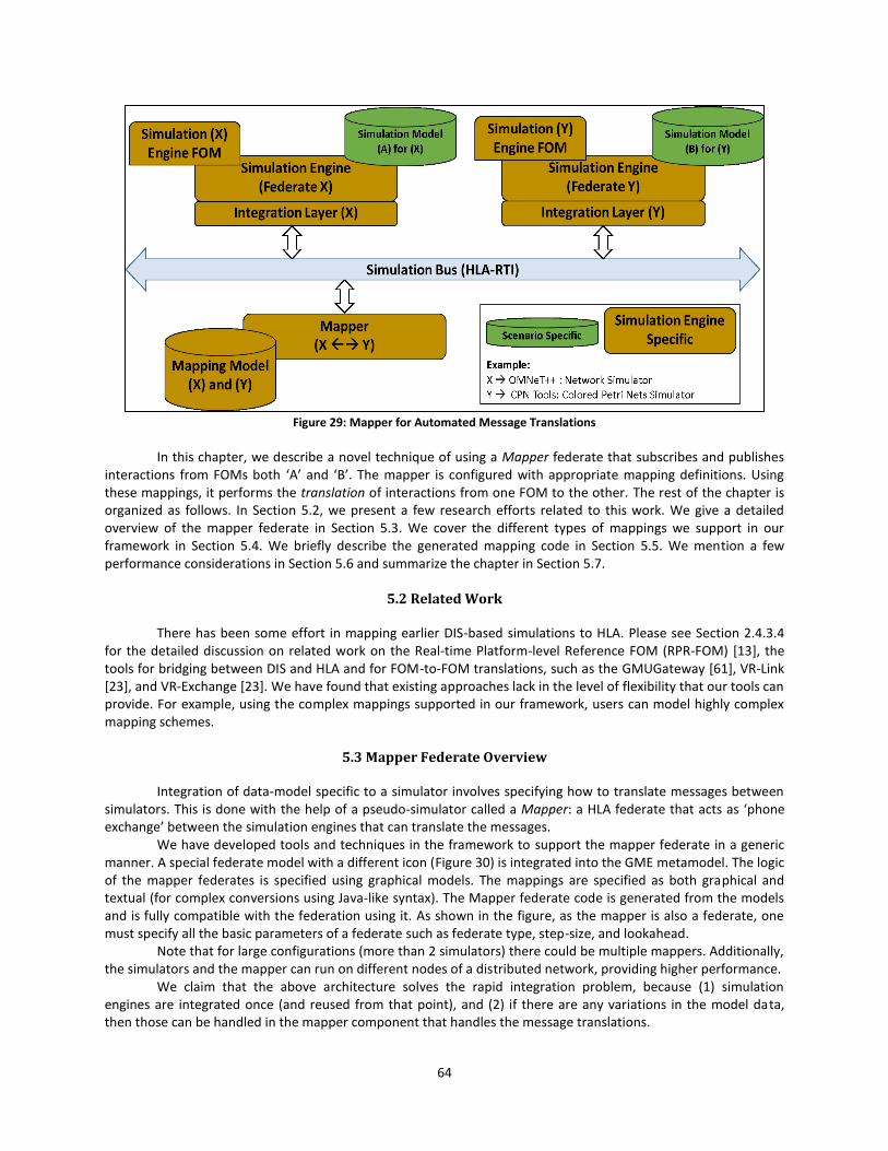
64

Figure 29: Mapper for Automated Message Translations

In this chapter, we describe a novel technique of using a Mapper federate that subscribes and publishes

interactions from FOMs both ‘A’ and ‘B’. The mapper is configured with appropriate mapping definitions. Using these mappings, it performs the translation of interactions from one FOM to the other. The rest of the chapter is organized as follows. In Section 5.2, we present a few research efforts related to this work. We give a detailed overview of the mapper federate in Section 5.3. We cover the different types of mappings we support in our framework in Section 5.4. We briefly describe the generated mapping code in Section 5.5. We mention a few performance considerations in Section 5.6 and summarize the chapter in Section 5.7.

5.2 Related Work

There has been some effort in mapping earlier DIS-based simulations to HLA. Please see Section 2.4.3.4 for the detailed discussion on related work on the Real-time Platform-level Reference FOM (RPR-FOM) [13], the tools for bridging between DIS and HLA and for FOM-to-FOM translations, such as the GMUGateway [61], VR-Link [23], and VR-Exchange [23]. We have found that existing approaches lack in the level of flexibility that our tools can provide. For example, using the complex mappings supported in our framework, users can model highly complex mapping schemes.

5.3 Mapper Federate Overview

Integration of data-model specific to a simulator involves specifying how to translate messages between simulators. This is done with the help of a pseudo-simulator called a Mapper: a HLA federate that acts as ‘phone exchange’ between the simulation engines that can translate the messages.

We have developed tools and techniques in the framework to support the mapper federate in a generic manner. A special federate model with a different icon (Figure 30) is integrated into the GME metamodel. The logic of the mapper federates is specified using graphical models. The mappings are specified as both graphical and textual (for complex conversions using Java-like syntax). The Mapper federate code is generated from the models and is fully compatible with the federation using it. As shown in the figure, as the mapper is also a federate, one must specify all the basic parameters of a federate such as federate type, step-size, and lookahead.

Note that for large configurations (more than 2 simulators) there could be multiple mappers. Additionally, the simulators and the mapper can run on different nodes of a distributed network, providing higher performance.

We claim that the above architecture solves the rapid integration problem, because (1) simulation engines are integrated once (and reused from that point), and (2) if there are any variations in the model data, then those can be handled in the mapper component that handles the message translations.

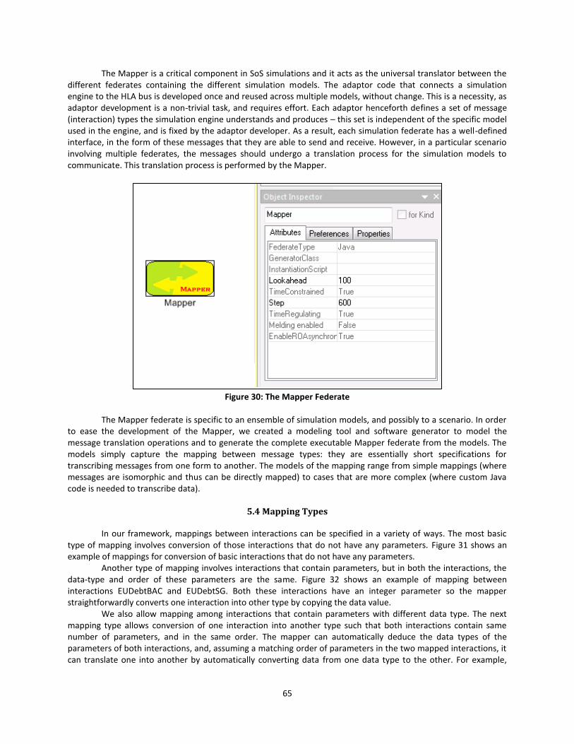
65

The Mapper is a critical component in SoS simulations and it acts as the universal translator between the different federates containing the different simulation models. The adaptor code that connects a simulation engine to the HLA bus is developed once and reused across multiple models, without change. This is a necessity, as adaptor development is a non-trivial task, and requires effort. Each adaptor henceforth defines a set of message (interaction) types the simulation engine understands and produces – this set is independent of the specific model used in the engine, and is fixed by the adaptor developer. As a result, each simulation federate has a well-defined interface, in the form of these messages that they are able to send and receive. However, in a particular scenario involving multiple federates, the messages should undergo a translation process for the simulation models to communicate. This translation process is performed by the Mapper.

Figure 30: The Mapper Federate

The Mapper federate is specific to an ensemble of simulation models, and possibly to a scenario. In order

to ease the development of the Mapper, we created a modeling tool and software generator to model the message translation operations and to generate the complete executable Mapper federate from the models. The models simply capture the mapping between message types: they are essentially short specifications for transcribing messages from one form to another. The models of the mapping range from simple mappings (where messages are isomorphic and thus can be directly mapped) to cases that are more complex (where custom Java code is needed to transcribe data).

5.4 Mapping Types

In our framework, mappings between interactions can be specified in a variety of ways. The most basic type of mapping involves conversion of those interactions that do not have any parameters. Figure 31 shows an example of mappings for conversion of basic interactions that do not have any parameters.

Another type of mapping involves interactions that contain parameters, but in both the interactions, the data-type and order of these parameters are the same. Figure 32 shows an example of mapping between interactions EUDebtBAC and EUDebtSG. Both these interactions have an integer parameter so the mapper straightforwardly converts one interaction into other type by copying the data value.

We also allow mapping among interactions that contain parameters with different data type. The next mapping type allows conversion of one interaction into another type such that both interactions contain same number of parameters, and in the same order. The mapper can automatically deduce the data types of the parameters of both interactions, and, assuming a matching order of parameters in the two mapped interactions, it can translate one into another by automatically converting data from one data type to the other. For example,

66

Figure 33 shows that when a FrenchTransferReceipt interaction is received by the mapper, which has a parameter ‘id’ of type ‘int’, it generates an equivalent interaction USTransferReceipt with no data conversion needed for the ‘id’ parameter, and an equivalent interaction IndianTransferReceipt with the value of ‘id’ converted to a ‘String’.

Figure 31: Mapping between Interactions with No Parameters

Figure 32: Mapping between Interactions with Parameters of Same Data Types

Figure 33: Mapping with Automatic Data Type Conversion

When a more complex set of interactions are involved that need a more complex translation logic than

the above three easier mechanisms, we allow user-defined Java-like code in the mapping models. The convention is used to denote the interactions mapped using a dollar sign followed by name of the modeling element representing the interaction in the mappings. Figure 34 shows an example of such complex mapping.

In this example user needs to translate interaction USMoneyGram into a NetworkPacket and vice versa. In the object models user has detailed parameter fields of these interactions. Creating a NetworkPacket interaction, for example, requires filling parameters such as senderHost, receiverHost, and packetType. The way to fill these parameter values are completely domain dependent and user is free to write any conversion code as shown in Figure 34. Note the use of dollar signs in the conversion code. This is a convention to refer to the participant

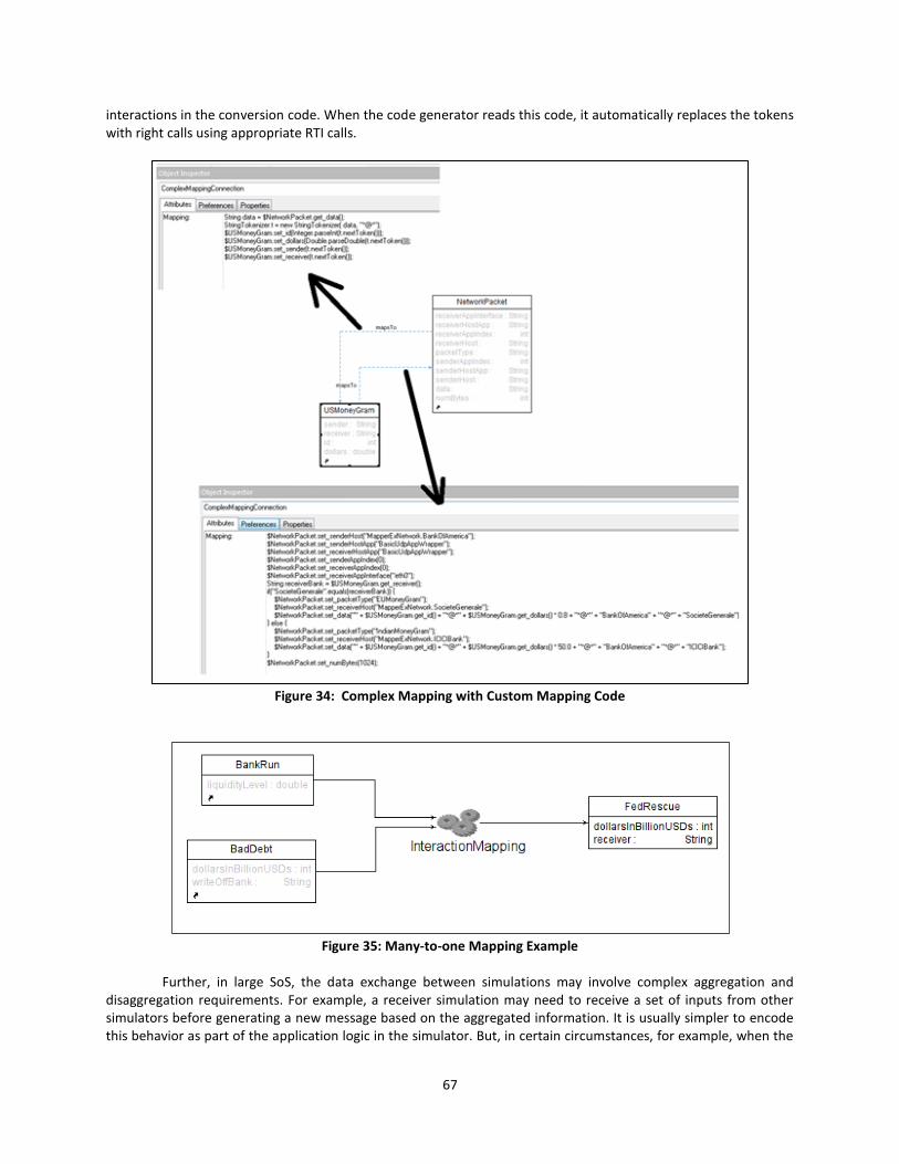
67

interactions in the conversion code. When the code generator reads this code, it automatically replaces the tokens with right calls using appropriate RTI calls.

Figure 34: Complex Mapping with Custom Mapping Code

Figure 35: Many-to-one Mapping Example

Further, in large SoS, the data exchange between simulations may involve complex aggregation and

disaggregation requirements. For example, a receiver simulation may need to receive a set of inputs from other simulators before generating a new message based on the aggregated information. It is usually simpler to encode this behavior as part of the application logic in the simulator. But, in certain circumstances, for example, when the

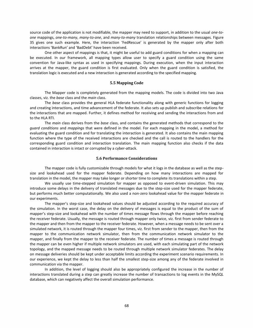
68

source code of the application is not modifiable, the mapper may need to support, in addition to the usual one-to-one mappings, one-to-many, many-to-one, and many-to-many translation relationships between messages. Figure 35 gives one such example. Here, the interaction ‘FedRescue’ is generated by the mapper only after both interactions ‘BankRun’ and ‘BadDebt’ have been received.

One other aspect of mappings is that, it might be useful to add guard conditions for when a mapping can be executed. In our framework, all mapping types allow user to specify a guard condition using the same convention for Java-like syntax as used in specifying mappings. During execution, when the input interaction arrives at the mapper, the guard condition is first evaluated. Only when the guard condition is satisfied, the translation logic is executed and a new interaction is generated according to the specified mapping.

5.5 Mapping Code

The Mapper code is completely generated from the mapping models. The code is divided into two Java classes, viz. the base class and the main class.

The base class provides the general HLA federate functionality along with generic functions for logging and creating interactions, and time advancement of the federate. It also sets up publish and subscribe relations for the interactions that are mapped. Further, it defines method for receiving and sending the interactions from and to the HLA RTI.

The main class derives from the base class, and contains the generated methods that correspond to the guard conditions and mappings that were defined in the model. For each mapping in the model, a method for evaluating the guard condition and for translating the interaction is generated. It also contains the main mapping function where the type of the received interactions are checked and the call is routed to the handlers for the corresponding guard condition and interaction translation. The main mapping function also checks if the data contained in interaction is intact or corrupted by a cyber-attack.

5.6 Performance Considerations

The mapper code is fully customizable through models for what it logs in the database as well as the step-size and lookahead used for the mapper federate. Depending on how many interactions are mapped for translation in the model, the mapper may take longer or shorter time to complete its translations within a step.

We usually use time-stepped simulation for mapper as opposed to event-driven simulation. This may introduce some delays in the delivery of translated messages due to the step-size used for the mapper federate, but performs much better computationally. We also used a non-zero lookahead value for the mapper federate in our experiments.

The mapper’s step-size and lookahead values should be adjusted according to the required accuracy of the simulation. In the worst case, the delay on the delivery of messages is equal to the product of the sum of mapper’s step-size and lookahead with the number of times message flows through the mapper before reaching the receiver federate. Usually, the message is routed through mapper only twice, viz. first from sender federate to the mapper and then from the mapper to the receiver federate. However, when a message needs to be sent over a simulated network, it is routed through the mapper four times, viz. first from sender to the mapper, then from the mapper to the communication network simulator, then from the communication network simulator to the mapper, and finally from the mapper to the receiver federate. The number of times a message is routed through the mapper can be even higher if multiple network simulators are used, with each simulating part of the network topology, and the mapped message needs to be routed through multiple network simulator federates. The delay on message deliveries should be kept under acceptable limits according the experiment scenario requirements. In our experience, we kept the delay to less than half the smallest step-size among any of the federate involved in communication via the mapper.

In addition, the level of logging should also be appropriately configured the increase in the number of interactions translated during a step can greatly increase the number of transactions to log events in the MySQL database, which can negatively affect the overall simulation performance.

69

5.7 Summary

In large SoS simulations, often some simulators need to use a pre-defined data model for their inputs and outputs. In such situations, it is not enough to use a commonly agreed data model among all simulators. Instead, we need to allow a simulator to interoperate with other simulators even if it uses its own data model. Whenever a curated simulation component (a simulator with fixed input and output data model for reusability) is used, mappings become essential for its interoperation with the other federates in the simulation. In this chapter, we described the tools and methods we developed for supporting legacy components through mapping methods. Essentially, these methods allow translation of messages between the commonly agreed data model and the one used by the legacy component.

The mapping methods we developed includes a custom modeling language to define mappings and a code generator to generate a mapper federate that executes synchronously with the rest of the simulation and translates messages as they are sent by other federates according to the specification provided in mapping models. The metamodel for this language is provided in Appendix A. The key features of this language are summarized as below:

1. Defining one or more mapper federates in a federation with their unique configuration of step-sizes and

lookahead values. 2. Defining the four types of mappings between interactions (see Section 5.4 for details):

a. Simple mapping between interactions with no parameters b. Simple mapping between interactions with parameters with same data types c. Simple mapping between interactions with different data types but with same number and order

of parameters d. Complex mapping between interactions that not only differ in the number and/or order of

parameters, but may also require user-defined logic for translating between them. 3. Defining guard condition on both simple and complex mappings to specify the conditions that must be

true for the mapping to take effect (i.e., translation of the mapped interaction). The guard condition is also defined using a Java-like syntax and can include the values of the parameters of the mapped interaction. The guard condition is executed every time a mapped interaction is received by the mapper federate and when it is satisfied (i.e., returns ‘true’), the translation logic is executed to translate the mapped interaction.

4. Defining InteractionMapping blocks for many-to-many mappings (see Section 5.4 for an example). The InteractionMapping block can include incoming connections from multiple interactions. Each of the connection from incoming interactions contains an ‘InputID’ field, which can be used in the translation logic defined using a Java-like syntax in the InteractionMapping block. This block can also have one or more outgoing connections to interactions that need to be generated because of the translation. Each of the outgoing connections contains an ‘OutputID’ field, which can be used in the translation logic to create the output interaction appropriately.

5. All input interactions for mappings are automatically subscribed by the mapper federate so that it can receive them from HLA-RTI at run-time. Similarly, all output interactions are automatically published by the mapper federate.

6. A code generator that takes the mapping specifications and generates the corresponding source code for a mapper federate. This needs to be compiled and executed as part of the federation for mappings to take effect. The techniques developed in this research have been used in almost all example experiments we

conducted and works with a reasonable performance. One of the shortcoming of this approach is that providing mapping logic in models is tedious and thus susceptible to human errors. In the future, we intend to extend our techniques with higher-level specification of rules to mitigate this issue.

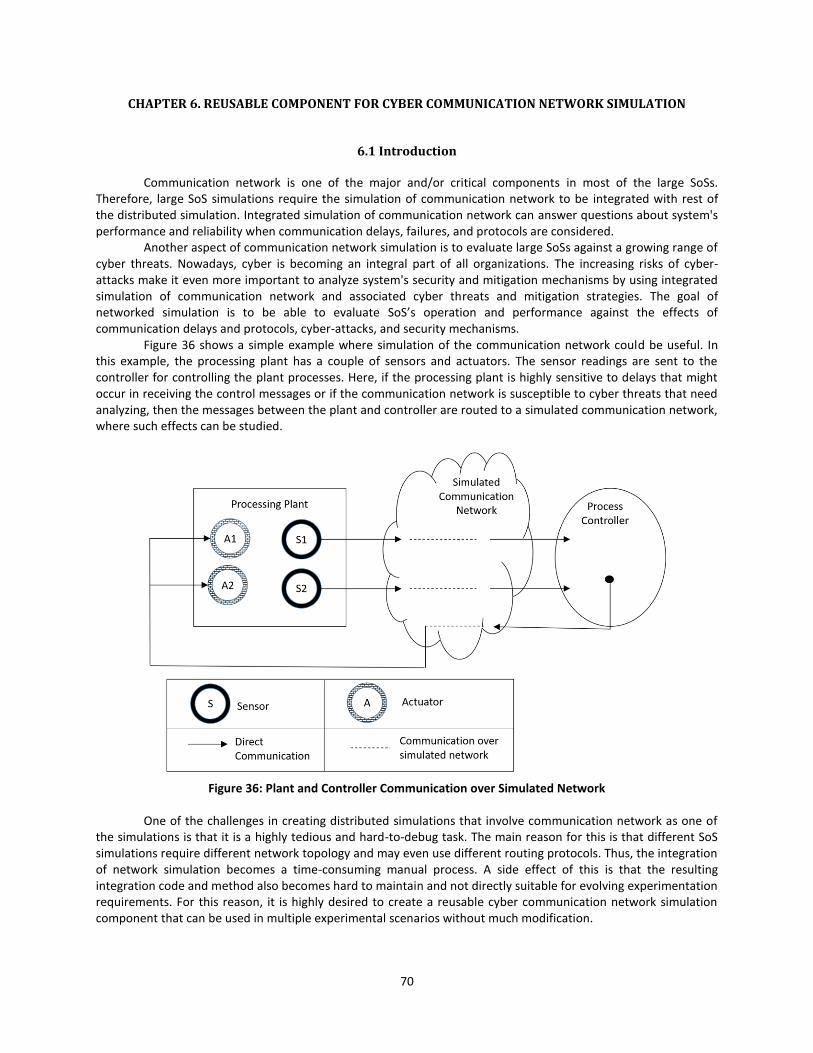
70

CHAPTER 6. REUSABLE COMPONENT FOR CYBER COMMUNICATION NETWORK SIMULATION

6.1 Introduction

Communication network is one of the major and/or critical components in most of the large SoSs. Therefore, large SoS simulations require the simulation of communication network to be integrated with rest of the distributed simulation. Integrated simulation of communication network can answer questions about system's performance and reliability when communication delays, failures, and protocols are considered.

Another aspect of communication network simulation is to evaluate large SoSs against a growing range of cyber threats. Nowadays, cyber is becoming an integral part of all organizations. The increasing risks of cyber-attacks make it even more important to analyze system's security and mitigation mechanisms by using integrated simulation of communication network and associated cyber threats and mitigation strategies. The goal of networked simulation is to be able to evaluate SoS’s operation and performance against the effects of communication delays and protocols, cyber-attacks, and security mechanisms.

Figure 36 shows a simple example where simulation of the communication network could be useful. In this example, the processing plant has a couple of sensors and actuators. The sensor readings are sent to the controller for controlling the plant processes. Here, if the processing plant is highly sensitive to delays that might occur in receiving the control messages or if the communication network is susceptible to cyber threats that need analyzing, then the messages between the plant and controller are routed to a simulated communication network, where such effects can be studied.

Figure 36: Plant and Controller Communication over Simulated Network

One of the challenges in creating distributed simulations that involve communication network as one of

the simulations is that it is a highly tedious and hard-to-debug task. The main reason for this is that different SoS simulations require different network topology and may even use different routing protocols. Thus, the integration of network simulation becomes a time-consuming manual process. A side effect of this is that the resulting integration code and method also becomes hard to maintain and not directly suitable for evolving experimentation requirements. For this reason, it is highly desired to create a reusable cyber communication network simulation component that can be used in multiple experimental scenarios without much modification.

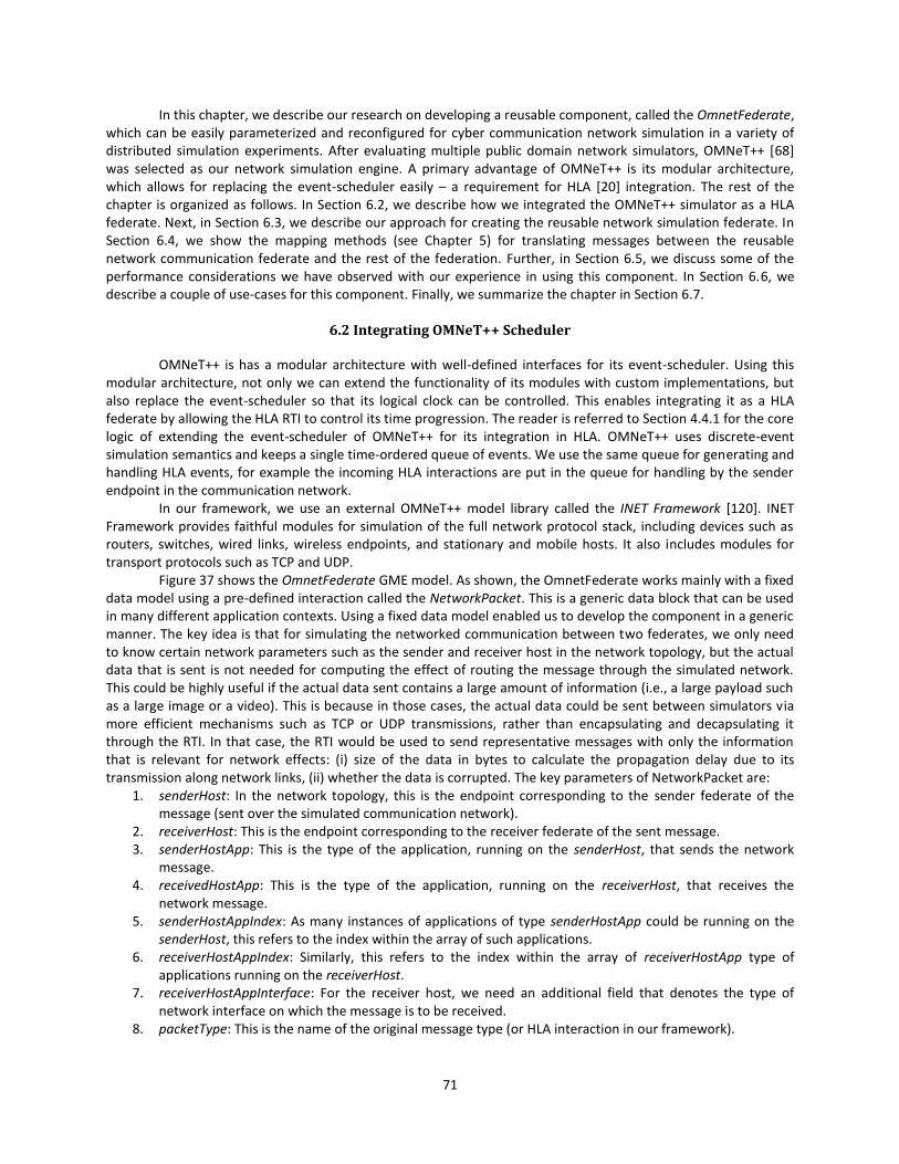
71

In this chapter, we describe our research on developing a reusable component, called the OmnetFederate, which can be easily parameterized and reconfigured for cyber communication network simulation in a variety of distributed simulation experiments. After evaluating multiple public domain network simulators, OMNeT++ [68] was selected as our network simulation engine. A primary advantage of OMNeT++ is its modular architecture, which allows for replacing the event-scheduler easily – a requirement for HLA [20] integration. The rest of the chapter is organized as follows. In Section 6.2, we describe how we integrated the OMNeT++ simulator as a HLA federate. Next, in Section 6.3, we describe our approach for creating the reusable network simulation federate. In Section 6.4, we show the mapping methods (see Chapter 5) for translating messages between the reusable network communication federate and the rest of the federation. Further, in Section 6.5, we discuss some of the performance considerations we have observed with our experience in using this component. In Section 6.6, we describe a couple of use-cases for this component. Finally, we summarize the chapter in Section 6.7.

6.2 Integrating OMNeT++ Scheduler

OMNeT++ is has a modular architecture with well-defined interfaces for its event-scheduler. Using this modular architecture, not only we can extend the functionality of its modules with custom implementations, but also replace the event-scheduler so that its logical clock can be controlled. This enables integrating it as a HLA federate by allowing the HLA RTI to control its time progression. The reader is referred to Section 4.4.1 for the core logic of extending the event-scheduler of OMNeT++ for its integration in HLA. OMNeT++ uses discrete-event simulation semantics and keeps a single time-ordered queue of events. We use the same queue for generating and handling HLA events, for example the incoming HLA interactions are put in the queue for handling by the sender endpoint in the communication network.

In our framework, we use an external OMNeT++ model library called the INET Framework [120]. INET Framework provides faithful modules for simulation of the full network protocol stack, including devices such as routers, switches, wired links, wireless endpoints, and stationary and mobile hosts. It also includes modules for transport protocols such as TCP and UDP.

Figure 37 shows the OmnetFederate GME model. As shown, the OmnetFederate works mainly with a fixed data model using a pre-defined interaction called the NetworkPacket. This is a generic data block that can be used in many different application contexts. Using a fixed data model enabled us to develop the component in a generic manner. The key idea is that for simulating the networked communication between two federates, we only need to know certain network parameters such as the sender and receiver host in the network topology, but the actual data that is sent is not needed for computing the effect of routing the message through the simulated network. This could be highly useful if the actual data sent contains a large amount of information (i.e., a large payload such as a large image or a video). This is because in those cases, the actual data could be sent between simulators via more efficient mechanisms such as TCP or UDP transmissions, rather than encapsulating and decapsulating it through the RTI. In that case, the RTI would be used to send representative messages with only the information that is relevant for network effects: (i) size of the data in bytes to calculate the propagation delay due to its transmission along network links, (ii) whether the data is corrupted. The key parameters of NetworkPacket are:

1. senderHost: In the network topology, this is the endpoint corresponding to the sender federate of the message (sent over the simulated communication network).

2. receiverHost: This is the endpoint corresponding to the receiver federate of the sent message. 3. senderHostApp: This is the type of the application, running on the senderHost, that sends the network

message. 4. receivedHostApp: This is the type of the application, running on the receiverHost, that receives the

network message. 5. senderHostAppIndex: As many instances of applications of type senderHostApp could be running on the

senderHost, this refers to the index within the array of such applications. 6. receiverHostAppIndex: Similarly, this refers to the index within the array of receiverHostApp type of

applications running on the receiverHost. 7. receiverHostAppInterface: For the receiver host, we need an additional field that denotes the type of

network interface on which the message is to be received. 8. packetType: This is the name of the original message type (or HLA interaction in our framework).

72

9. data: This is an encoding of the content of the original HLA interaction sent by the sender federate. The original interaction can be recreated using this information along with the knowledge of its corresponding packetType.

10. numBytes: This is used to calculate the propagation delay when the network message is relayed within the simulated network between senderHost and receiverHost.

Figure 37: Fixed Data Model for OmnetFederate

Scalability of network simulation is a key issue particularly when large number of network messages need

to be simulated. For example, in an experiment that simulates huge communication network traffic on a server node, one might need to generate a large set of such messages and simulate their transmission in the simulated network. In our framework, we keep the heavy message traffic as much as possible inside the OMNeT++ simulator. Only a high-level application layer interface is provided for HLA that results in a much lighter message traffic along the HLA communication path and thereby improved performance of the entire simulation.

6.3 Creating a Reusable Network Simulation Federate

In order to implement the reusable functionality of the OmnetFederate, we extended the INET Framework’s basic UDP application with functions to respond to relay the messages to configured destinations. We also created a new module called HLAInterface that sends and receives interactions from/to the RTI and routes them to network hosts corresponding to the sender and receiver federates that communicate through the simulated network. An OMNeT++ model consists of hierarchically nested modules – containing the model’s algorithms and/or other modules – that communicate via messages. Gates are a module’s input and output interfaces for receiving and sending messages. OMNeT++ supports directIn input gates for messages that do not incur a propagation delay. We used such a gate for messages sent between the HLAInterface and the applications running on sender and receiver hosts. To include this customization, we extended many commonly used modules of the INET Framework such as StandardHost, WirelessHost, Router, IP, NetworkLayer, DHCPRouter, DHCPClient, and DHCPServer. Note that this customization preserves all of the existing module parameters, but adds additional parameters for custom functionality of the extended modules.

The HLAInterface module contains the core OmnetFederate functionality and must be included in any network topology used in an experiment. The key parameters of the HLAInterface module include federate-step-size, federate-lookahead, federate-name, and federation-name. The C++ class implementing the HLAInterface is derived from both the HLA federate base class from the Portico RTI [21] and cSimpleModule class in OMNeT++. The class implements all the HLA federate functions such as for registering publish and subscribe relations with HLA interactions, receiving and sending HLA interactions, and logic for handling time synchronization with the RTI.

73

6.4 Mappings for NetworkPacket Encapsulation and Decapsulation

The reusability of the cyber communication network simulation component, called OmnetFederate, stems from its use of a pre-defined data model for data exchange on the HLA RTI. Specifically, the OmnetFederate register to publish and subscribe the interaction called NetworkPacket. This allows for implementing OmnetFederate in a generic manner so that it can be used without much modification in different experiment scenarios (with different scenario-specific network topology, network routes, and network routing protocols). However, different scenarios use domain-specific data models for describing the inputs and outputs among different simulators (i.e. HLA federates) it uses. Therefore, we must use the mapping methods described in Chapter 5 for automatically translating interactions between the scenario-specific data model and NetworkPacket. This is accomplished by specifying the complex mapping between the corresponding HLA interactions and the NetworkPacket interaction in scenario models. As was illustrated previously in Figure 34, the complex mapping requires the user to provide translation logic in the form of a Java-like syntax in the models. The translation logic converts the scenario HLA interactions into NetworkPacket and vice versa. For creating the NetworkPacket interaction, values of its parameters such as senderHost, receiverHost, and packetType, must be appropriately provided.

6.5 Performance Considerations

The OmnetFederate can be customized for the step-size and lookahead values it will use as a HLA federate. In addition, the level of logging in the MySQL database can be fully configured. We implemented the component to minimize the network traffic on the HLA bus by limiting maximum traffic inside OMNeT++. This helps with increasing the performance of the simulation. However, the step-size, lookahead, and the logging levels can still significantly affect its performance, especially if there are several HLA interactions that are to be sent over the simulated network. Another important consideration is that the time-stepped simulation may cause extra delays in the HLA interactions. Thus, the federate's step-size and lookahead values should be adjusted according to the required accuracy of the simulation. The delay incurred due to time-stepped simulation should be small enough such that the cyber effects desired through networked co-simulation are not affected significantly. In general, the increase in federate’s step-size and lookahead directly increases the delay encountered in delivering the message to the receiver federates, thereby decreasing the overall simulation accuracy.

OMNeT++ allows executing the simulator in various modes, viz. command-line (or non-GUI), slow, fast, and express. We have observed that the command-line mode is the fastest among all. In GUI mode, the various modes can be customized for updating display at different number of steps. Accordingly, the frequency of updates will change and can significantly affect the performance of the simulation. These modes in GUI mode can be changed and updated even when a simulation is still in progress.

It is important to note here that OMNeT++ is a highly sophisticated simulator with a very high fidelity of simulation that includes the full stack of network layers. The simulation internally uses nanosecond time-resolution accuracy. However, at the SoS level simulation, the impact of cyber threats and node failures is more interesting than the precise detail of delays. We utilize this by limiting the majority of HLA traffic to the main application-level data exchanges. However, when significant amount of low-level traffic is simulated inside OMNeT++, such as when simulating a large traffic-generation routine or the use of radio communications, the performance of the overall simulation can be impacted.

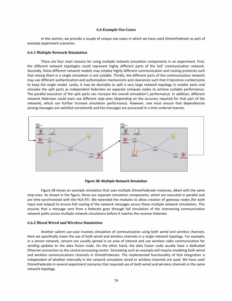
74

6.6 Example Use-Cases

In this section, we provide a couple of unique use-cases in which we have used OmnetFederate as part of example experiment scenarios.

6.6.1 Multiple Network Simulation

There are four main reasons for using multiple network simulation components in an experiment. First, the different network topologies could represent highly different parts of the SoS’ communication network. Secondly, these different network models may employ highly different communication and routing protocols such that mixing them in a single simulation is not suitable. Thirdly, the different parts of the communication network may use different authentication and authorization mechanisms and clearances such that it becomes cumbersome to keep the single model. Lastly, it may be desirable to split a very large network topology in smaller parts and simulate the split parts as independent federates on separate compute nodes to achieve scalable performance. The parallel execution of the split parts can increase the overall simulation’s performance. In addition, different network federates could even use different step-sizes (depending on the accuracy required for that part of the network), which can further increase simulation performance. However, one must ensure that dependencies among messages are satisfied consistently and the messages are processed in a time-ordered manner.

Figure 38: Multiple Network Simulation

Figure 38 shows an example simulation that uses multiple OmnetFederate instances, albeit with the same

step-sizes. As shown in the figure, these are separate simulation components, which are executed in parallel and are time-synchronized with the HLA RTI. We extended the modules to allow creation of gateway nodes (for both input and output) to ensure full routing of the network messages across these multiple network simulations. This ensures that a message sent from a federate goes through full simulation of the intervening communication network paths across multiple network simulations before it reaches the receiver federate.

6.6.2 Mixed Wired and Wireless Simulation

Another salient use-case involves simulation of communication using both wired and wireless channels. Here we specifically mean the use of both wired and wireless channels in a single network topology. For example, in a sensor network, sensors are usually spread in an area of interest and use wireless radio communication for sending updates to the data fusion node. On the other hand, the data fusion node usually have a dedicated Ethernet connection to the central processing center. Simulating such an example will require modeling both wired and wireless communications channels in OmnetFederate. The implemented functionality of HLA integration is independent of whether internally in the network simulation wired or wireless channels are used. We have used OmnetFederate in several experiment scenarios that required use of both wired and wireless channels in the same network topology.

75

6.7 Summary

Communication network is one of the major and/or critical components in most of the large SoSs as it spans across many independent systems. A SoS’ performance and reliability could be severely impacted due to communication delays, failures, and protocols used. Therefore, integrated simulation of the communication network is necessary for comprehensive evaluation of large SoSs. In this chapter, we described our research on developing a reusable cyber communication network simulation component called OmnetFederate. OmnetFederate has an extensible architecture that allows it to be used in many different experiment scenarios, and makes it easier to extend for additional networking behaviors and protocols.

OMNeT++ is a highly sophisticated and widely used communication network simulation tool. It supports simulation accuracy up to nanoseconds. It provides configurable and parametric modules for the full stack of network layers. The speed of network simulation depends on how large is the network topology and how many messages are sent across nodes in the simulated network. This is much slower than a real, physical transmission of network packets because the simulated network requires computation at all stages and layers through which a network packet flows. For example, in OMNeT++, computation is required to calculate and maintain the variables in associated OMNeT++ modules across the networking layers. Thus, OMNeT++, being a low-level network simulator, could become computationally expensive. However, in the context of large SoS simulations, it is typically sufficient to model only the impact of higher-level cyber effects such as packet flooding, network link drops, or node failures, which enables using the network simulator with an acceptable performance.

As suggested above, not all network characteristics can be simulated to a high degree of precision due to performance constraints. For example, a faithful DDoS simulation may require very large number of packet transmissions that it becomes computationally too expensive in a simulation. Use of physical hardware based network affects is also another example where network simulation is not applicable. In these situations, network emulation [69] can be used; where a physical hardware is used for transmitting network-packets physically (see Section 2.1.8 and Section 2.2.1.5 for more on network emulation).

76

CHAPTER 7. PARTITIONING DYNAMIC MODELS FOR EFFICIENT CO-SIMULATION

7.1 Introduction

Large dynamical models often have many sub-component models that exhibit different rate dynamics. This effectively means that some parts of the models could be executed much faster (i.e., take less computation time on average per step) than the other parts. The primary reason for this is the nature of equations that represent the model’s behavior. Many models use differential equations and differential algebraic equations to represent their behavior. These equations often use higher order derivatives of variables, which can cause large changes in dependent variables even when the independent variables are changed only slightly. Therefore, when these models are simulated, a rather small step-size must be used to prevent large discontinuities in the dependent variables that can lead the model into an unstable state. Consequently, when the entire model is executed as one simulation component, the entire model must be executed at the smallest step-size among the maximum step-sizes allowable (i.e., one that still keeps it stable) in any of its constituent sub-component models.

It can be easily seen that if such models could be partitioned into different sampling rate (i.e., step-size) groups, then different groups could be executed at different step-sizes, thereby relaxing the constraint that the entire model must be executed at the maximum step-size that keeps all sub-component models stable. However, this is challenging for three key reasons:

1. First, we need a method for partitioning the model into sub-component models across different sampling rate groups such that dependencies of variables are well captured and modeled. For example, consider a large dynamical model developed using Bond graphs [73]. If we split the model into four parts, we need to capture the flow of energy appropriately such that input-output relationship among the split models still maintain the balance of effort and flow across the bonds.

2. The second challenge is that once the model is split into sub-component models, their execution must happen in parallel. Their parallel execution can provide some computation benefit because some of them could potentially be executed at much larger step-size than the one requiring the smallest step-size. However, when these split models are executed in parallel the outputs from one must be relayed effectively and timely to the receiver models.

3. Lastly, the execution of the sub-component models must be coordinated such that they all execute in a time-synchronized manner. This is different from simply parallel execution and needed because these sub-component models are effectively parts of a single larger model and for maintaining consistent run-time behavior their execution must be synchronized. A small deviation in timing among any of the sub-component models could lead to large unintended behavioral discrepancies in the model execution.

7.1.1 Approach

We approach the problem by leveraging the Functional Mock-up Interface (FMI) [5] standard for splitting the models across sampling rate boundaries and executing the split sub-component models as Functional Mock-up Units (FMUs) in a co-simulation. First, we split the model that exhibits different rate dynamics in different parts of the model across sampling rate boundaries. Next, we export each split sub-component model as an FMU (i.e., a .zip file containing the corresponding model description XML file and binary files for executing its behavior). We then abstract each split sub-component model as a HLA-federate in the overall system-of-systems integrated simulation. Here, we also model the input and output relationships of the sub-component models using HLA-interactions and create appropriate publish and subscribe relations in the model. We call these types of HLA-federates as FMU-federates in our simulation integration framework.

Our solution uses the Modelica modeling and simulation tool called Dymola [27] and Modelica models as candidate for splitting and exporting as FMUs. However, the FMI-standard is implementation agnostic such that the binaries could be exported in many different ways (e.g., from a MATLAB/Simulink model or written manually using C/C++). Thus, our solution should be applicable in a similar way to other tools that can simulate Modelica models.

According to the naming conventions used while exporting the part of the model as an FMU file, the input and output variables will be named differently. For example, if a variable is an output from one part of the model

77

and serves as an input in the other part of the model, then when the model is split in those two parts, the names of input and output variables may be different in each FMU depending on the tool used for the export. Therefore, we use the mapping methods (described in Chapter 5) to map outputs of the sending split models to inputs of the receiving split models. Use of mapping methods does introduce artificial delays between the time a variable is outputted and the time it is updated in the receiver model. Consistent simulation can still be achieved, however, if these delays are kept small. Further, the benefits in simulation performance can outweigh the small errors introduced due to these delays. Note that an FMU-federate can be both a sender of a variable and a receiver of another variable (presumably the output of other HLA-federate). In most cases, we can use the SimpleMappingConnection for creating direct mapping from outputs to inputs. However, in some cases, when a variable’s value needs to be aggregated, divided, or multiplexed, a ComplexMappingConnection with detailed transformation logic can be used for creating the mappings.

7.1.2 Chapter Organization

In this chapter, we first present our research paper titled “Model-Based Integration Platform for FMI Co-Simulation and Heterogeneous Simulations of Cyber-Physical Systems”. Secondly, we describe the status of current software implementation for automating the development and execution of FMU-federates. Next, we present a systematic method to use the technique of splitting complex dynamical models across sampling rate boundaries effectively. Finally, we provide a summary of the work.

78

7.2 Research Paper on Integrating FMI Co-Simulations

Title: Model-Based Integration Platform for FMI Co-Simulation and Heterogeneous Simulations of Cyber-

Physical Systems Authors: Himanshu Neema, Jesse Gohl, Zsolt Lattmann, Janos Sztipanovits, Gabor Karsai, Sandeep Neema,

Ted Bapty, John Batteh, Hubertus Tummescheit Note: This paper was published in the 10th International Modelica Conference, March 10-12, 2014, Lund,

Sweden. In this section, we reproduce almost the literal copy of this paper, with only minor terminology changes to match those used in the rest of the dissertation.

Abstract: Virtual evaluation of complex Cyber-Physical Systems (CPS) with a number of tightly integrated

domains such as physical, mechanical, electrical, thermal, cyber, etc. demand the use of heterogeneous simulation environments. Our previous effort with C2 Wind Tunnel (C2WT) attempted to solve the challenges of evaluating these complex systems as-a-whole, by integrating multiple simulation platforms with varying semantics and integrating and managing different simulation models and their interactions. Recently, a great interest has developed to use Functional Mockup Interface (FMI) for a variety of dynamics simulation packages, particularly in Commercial Off-The-Shelf (COTS) tools. Leveraging the C2WT effort on effective integration of different simulation engines with different Models of Computation (MoCs), we propose, in this paper, to use the proven methods of High-Level Architecture (HLA)-based model and system integration. We identify the challenges of integrating Functional Mockup Unit for Co-Simulation (FMU-CS) in general and via HLA and present a novel model-based approach to rapidly synthesize an effective integration. The approach presented provides a unique opportunity to integrate readily available FMU-CS components with various specialized simulation packages to rapidly synthesize HLA-based integrated simulations for the overall composed Cyber-Physical Systems.

7.2.1 Introduction

Cyber-Physical Systems (CPS) [1] are composed of several collaborating physical and computing components that interact through embedded communication capabilities. These systems require advanced integration of abstractions and techniques that have been developed over the past years in disparate areas such as cyber systems that rely heavily on computation and networking and physical systems that employ various engineering methods in domains such as mechanical, thermal, electrical, electronic, hydraulic, thermal, biological, and acoustic.

Analysis of Cyber-Physical Systems poses unique challenges due to the heterogeneity of components and interactions [95]. The fundamental differences in the characteristics of these different physical and computation processes lead to a huge spectrum of modeling methods. For example, some components can be easily described by differential equations, while others like communication networks typically require Discrete-Event Simulation techniques. As such, several simulation tools and techniques are needed for CPS simulation and analysis. This further necessitates an over-arching CPS model and system integration platform that is model-based and supports rapid synthesis of distributed heterogeneous CPS simulations.

Co-Simulation (Co-operative Simulation) is a simulation method that permits simulating individual components using different simulation tools simultaneously and collaboratively. Individual simulation tools exchange information such as individual system variables and their values, time-steps for synchronization, and control signals for orchestrating the co-operative simulation. In this way, engineers can use different simulation tools together to create virtual prototypes of entire Cyber-Physical Systems. In practice, however, significant challenges remain with regard to the syntax and semantics of model and system integration.

In the Co-Simulation domain, a recent effort by the MODELISAR ITEA2 project that develops a tool independent standard called the Functional Mock-up Interface (FMI) [4] [5] [6] has gained significant influence, more prominently in the automotive industry. The FMI standard provides a well-defined set of function calls to specify simulation components. FMI-compliant simulations pack shared libraries that can be executed using the

79

standardized function calls and the model execution must adhere to the rules of the standard. These function calls span all stages of the model execution, viz. initialization, configuration, access, modification, and manipulation.

The strength of FMI lies in the fact that all simulation tools participating in the Co-Simulation follow the defined standard and as such provides for standardized access to model equations. This permits coupling of Continuous-Time and Discrete-Time systems that are part and parcel of Cyber-Physical Systems. In some ways, this is also a limitation because not all simulation tools are amenable to support all of the strictly specified FMI function calls.

Another key requirement for Co-Simulation via FMI is to also develop a master algorithm that orchestrates the steps of Co-Simulation. Master algorithms must control the data exchange between subsystems and synchronize their individual simulations according to the requirements of the integrated simulation of the overall Cyber-Physical System. Although the FMI standard does not describe or limit the implementation of the master algorithm, the algorithm requirements and features often limit its implementation as a centralized orchestrator that can communicate effectively with all participating subsystems. Centralized nature not only can become a performance bottleneck, it can also serve as a single point of failure in the distributed simulation’s computational infrastructure.

Furthermore, as Cyber-Physical Systems involve vastly different sub-domains and physical processes that vary greatly in the execution frequency at which they need to run. This leads to significantly different dynamic response characteristics in terms of frequencies. For example, mechanical components of a complex CPS often have much slow frequency responses compared to fast electronic components. Single standalone monolithic model of a CPS therefore suffers heavily with solver inefficiencies. These systems are generally highly complex and have a significant non-linearity and discontinuities, which further adds to inefficiencies of solvers. Taking subsystems apart and using different solver step-sizes offers a potential solution. However, multirate composition also introduces some inefficiencies due to clock management, composition restrictions, data exchange, and potential stability issues if the system is split at the wrong place.

Another effort developed by U.S. Modeling and Simulation Coordination Office (M&S CO) is the High Level Architecture (HLA) [20]. The HLA provides a specification of a common technical architecture for modeling and simulation with a primary goal to facilitate interoperability among simulations and to promote re-use of simulations and their components. The HLA comprises of three major components: HLA rules, HLA interface specification, and HLA object model template [6]. With these rules, the HLA standardizes run-time support for various tasks, such as coordinated time evolution, message passing and shared object management. The key difference from FMI is that HLA regards individual simulation components at the level of processes as opposed to libraries. This enables broader integration of different simulation tools with different Models of Computation. Even Functional Mock-up Units can be integrated as a participating simulation tool in the overall integrated simulation of the Cyber-Physical Systems.

Another key benefit of HLA is that its Distributed Discrete Event model of computation allows full flexibility to individual subsystems in using any internal solver and model of computation. Moreover, this flexibility permits multirate simulations by design.

However, the HLA standard also lacks some key facilities for developing integrated distributed heterogeneous simulations. For example, the HLA standard does not formalize methods for developing interactions and objects used by HLA federates and it does not provide facilities for easily moving simulations from one computational node to other. Consequently, HLA-based simulations also require a significant amount of tedious and error-prone hand-developed integration code.

Achieving the integrated simulation of Cyber-Physical Systems require effective integration of a huge spectrum of models of physical processes, communication systems, exchanged information, and control mechanisms. As detailed above, the approaches of FMI and HLA both have their advantages and some key limitations. The approach of using HLA as a master algorithm enables use of FMUs in a Co-Simulation environment while also providing flexibility of using other types of non-FMU simulations [96]. The resulting framework can provide a much broader scale of simulation tools that can be used in the integrated simulation of Cyber-Physical Systems. However, several gaps need to be filled in order to develop a platform that enables this integration in an efficient manner. A single efficient model-based platform is needed that:

Enables modeling of interactions and shared objects between simulation tools

Enables modeling of integration of systems with their data exchange mechanisms

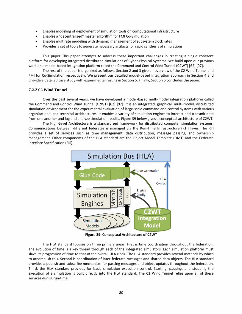
80

Enables modeling of deployment of simulation tools on computational infrastructure

Enables a "decentralized" master algorithm for FMI Co-Simulation

Enables multirate modeling with dynamic management of subsystem clock rates

Provides a set of tools to generate necessary artifacts for rapid synthesis of simulations This paper This paper attempts to address these important challenges in creating a single coherent

platform for developing integrated distributed simulations of Cyber-Physical Systems. We build upon our previous work on a model-based integration platform called the Command and Control Wind Tunnel (C2WT) [62] [97].

The rest of the paper is organized as follows. Section 2 and 3 give an overview of the C2 Wind Tunnel and FMI for Co-Simulation respectively. We present our detailed model-based integration approach in Section 4 and provide a detailed case study with experimental results in Section 5. Finally, Section 6 concludes the paper.

7.2.2 C2 Wind Tunnel

Over the past several years, we have developed a model-based multi-model integration platform called the Command and Control Wind Tunnel (C2WT) [62] [97]. It is an integrated, graphical, multi-model, distributed simulation environment for the experimental evaluation of large-scale command and control systems with various organizational and technical architectures. It enables a variety of simulation engines to interact and transmit data from one another and log and analyze simulation results. Figure 39 below gives a conceptual architecture of C2WT.

The High-Level Architecture is a standardized framework for distributed computer simulation systems. Communications between different federates is managed via the Run-Time Infrastructure (RTI) layer. The RTI provides a set of services such as time management, data distribution, message passing, and ownership management. Other components of the HLA standard are the Object Model Template (OMT) and the Federate Interface Specification (FIS).

Figure 39: Conceptual Architecture of C2WT

The HLA standard focuses on three primary areas. First is time coordination throughout the federation.

The evolution of time is a key thread through each of the integrated simulators. Each simulation platform must slave its progression of time to that of the overall HLA clock. The HLA standard provides several methods by which to accomplish this. Second is coordination of inter-federate messages and shared data objects. The HLA standard provides a publish-and-subscribe mechanism for passing messages and object updates throughout the federation. Third, the HLA standard provides for basic simulation execution control. Starting, pausing, and stopping the execution of a simulation is built directly into the HLA standard. The C2 Wind Tunnel relies upon all of these services during run-time.

81

As HLA is an accepted standard, a number of commercial, academic, and alternate RTI implementations are available. Currently, we use the Portico RTI [21] – which provides support for both C++ and Java clients and is compliant with version 1.3 of the HLA standard.

The HLA provides a standard for the RTI that supports the coordinated execution of distributed simulations. However, designing the model integration, coding the platform-to-RTI integration code, and testing and deploying all of the various run-time components across multiple platform-specific simulation tools is a highly challenging task. C2WT provides a solution to this simulation integration problem. It provides a holistic modeling and management environment built around a custom Domain-Specific Modeling Language (DSML) [98], implemented in Generic Modeling Environment (GME) [98], and a related suite of model interpreters to coordinate between the integration model and the platform-specific simulation tools involved in the overall environment. It facilitates the rapid development of integration models and use of these models throughout the lifecycle of the simulated environment. With simulation engine specific model configurations and experiment specific deployment modeling, it enables significant automation in the development of integrated distributed simulation. With integration modeling support and various sophisticated generation tools, C2WT provides a robust platform for users to rapidly model and synthesize complex, heterogeneous, command and control simulations.

7.2.3 FMI for Co-Simulation

Functional Mock-up Interface (FMI) [4] [5] [6] was initiated and organized by Daimler AG within the ITEA2 project MODELISAR [4]. The FMI standard consists of two main parts. The first part is FMI for Model Exchange, which standardizes the distribution of a dynamic system model in the form of generated C-Code as an input/output block to other simulation environments. The second part is FMI for Co-Simulation, which standardizes the mechanisms for coupling of two or more simulation tools in a co-simulation environment.

The key idea is to have a discrete set of communication points only, at which times the subsystems exchange any data. Outside of these points, the subsystems are executed independently. The data exchange is controlled by a master system that also manages time synchronization of subsystems.

The FMI Co-simulation master simulator couples the subsystem simulators through a zip-archive. This zip-archive contains shared library files (.DLL, .SO) that conform to the function call specifications given in the standard. Each zip-archive also contains a XML file that provides meta-data and further details of the model such as default start and stop times, variable types, units, tool specific data, parameter and variable names and attributes. The XML also contains specification for executing the model as a shared library during a simulation run (CoSimulation_Standalone) or by importing a slave tool wrapper and interfacing it with the external tool (CoSimulation_Tool).

7.2.4 Model-Based Integration

One of the primary contributions of our effort is our focus on developing a completely model-based integration approach. Our efforts leverage the Generic Modeling Environment (GME) [98] tool suite for designing the integration model DSML [98] and HLA [20] to provide run-time support as the “simulation bus”.

7.2.4.1 Needs and Challenges

Cyber-Physical Systems [1] [95] are highly complex and their simulation spans a multitude of computational domains and specializations. A large number of tools exist that have been developed for specific aspects of CPSs. A variety of tools exists even for a single aspect of CPSs. For example, many special purpose simulation tools exist to model and analyze vehicle dynamics or for switching mechanisms of hybrid drivetrains. As such, the integration platform must be open toward use of any tool that may be required for some component/aspect of the CPS simulation.

A subtle problem in using multiple simulation tools in an integrated simulation is that they tend to use many different Models of Computation (MoC). For example, Discrete-Event, Discrete-Time, Continuous-Time, Synchronous Dataflow, are among the many MoCs used. Each MoC has a specific mechanism for time progression and event handling. The integration platform must be able to handle tools that use different MoCs in highly flexible manner. The integrated system must respect time synchronization with other simulation tools as well as the causality of events must be preserved. In addition to system integration, the platform must also enable integration

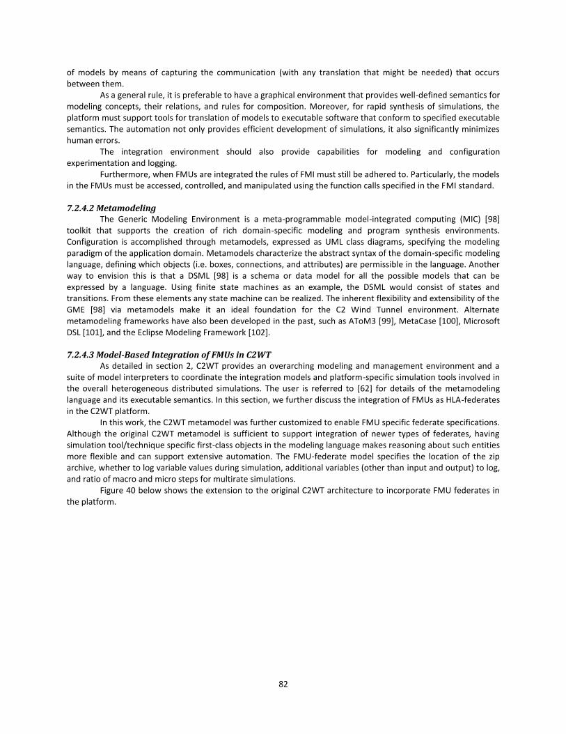
82

of models by means of capturing the communication (with any translation that might be needed) that occurs between them.

As a general rule, it is preferable to have a graphical environment that provides well-defined semantics for modeling concepts, their relations, and rules for composition. Moreover, for rapid synthesis of simulations, the platform must support tools for translation of models to executable software that conform to specified executable semantics. The automation not only provides efficient development of simulations, it also significantly minimizes human errors.

The integration environment should also provide capabilities for modeling and configuration experimentation and logging.

Furthermore, when FMUs are integrated the rules of FMI must still be adhered to. Particularly, the models in the FMUs must be accessed, controlled, and manipulated using the function calls specified in the FMI standard.

7.2.4.2 Metamodeling

The Generic Modeling Environment is a meta-programmable model-integrated computing (MIC) [98] toolkit that supports the creation of rich domain-specific modeling and program synthesis environments. Configuration is accomplished through metamodels, expressed as UML class diagrams, specifying the modeling paradigm of the application domain. Metamodels characterize the abstract syntax of the domain-specific modeling language, defining which objects (i.e. boxes, connections, and attributes) are permissible in the language. Another way to envision this is that a DSML [98] is a schema or data model for all the possible models that can be expressed by a language. Using finite state machines as an example, the DSML would consist of states and transitions. From these elements any state machine can be realized. The inherent flexibility and extensibility of the GME [98] via metamodels make it an ideal foundation for the C2 Wind Tunnel environment. Alternate metamodeling frameworks have also been developed in the past, such as AToM3 [99], MetaCase [100], Microsoft DSL [101], and the Eclipse Modeling Framework [102].

7.2.4.3 Model-Based Integration of FMUs in C2WT

As detailed in section 2, C2WT provides an overarching modeling and management environment and a suite of model interpreters to coordinate the integration models and platform-specific simulation tools involved in the overall heterogeneous distributed simulations. The user is referred to [62] for details of the metamodeling language and its executable semantics. In this section, we further discuss the integration of FMUs as HLA-federates in the C2WT platform.

In this work, the C2WT metamodel was further customized to enable FMU specific federate specifications. Although the original C2WT metamodel is sufficient to support integration of newer types of federates, having simulation tool/technique specific first-class objects in the modeling language makes reasoning about such entities more flexible and can support extensive automation. The FMU-federate model specifies the location of the zip archive, whether to log variable values during simulation, additional variables (other than input and output) to log, and ratio of macro and micro steps for multirate simulations.

Figure 40 below shows the extension to the original C2WT architecture to incorporate FMU federates in the platform.

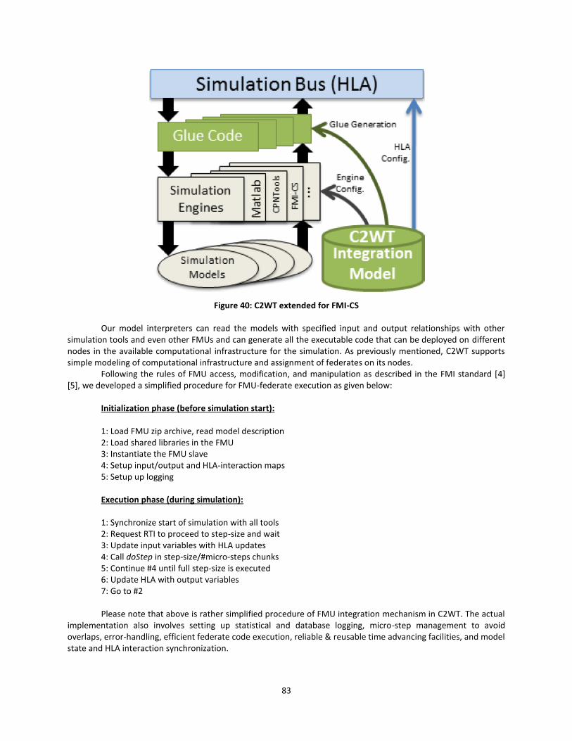
83

Figure 40: C2WT extended for FMI-CS

Our model interpreters can read the models with specified input and output relationships with other

simulation tools and even other FMUs and can generate all the executable code that can be deployed on different nodes in the available computational infrastructure for the simulation. As previously mentioned, C2WT supports simple modeling of computational infrastructure and assignment of federates on its nodes.

Following the rules of FMU access, modification, and manipulation as described in the FMI standard [4] [5], we developed a simplified procedure for FMU-federate execution as given below:

Initialization phase (before simulation start): 1: Load FMU zip archive, read model description 2: Load shared libraries in the FMU 3: Instantiate the FMU slave 4: Setup input/output and HLA-interaction maps 5: Setup up logging Execution phase (during simulation): 1: Synchronize start of simulation with all tools 2: Request RTI to proceed to step-size and wait 3: Update input variables with HLA updates 4: Call doStep in step-size/#micro-steps chunks 5: Continue #4 until full step-size is executed 6: Update HLA with output variables 7: Go to #2 Please note that above is rather simplified procedure of FMU integration mechanism in C2WT. The actual

implementation also involves setting up statistical and database logging, micro-step management to avoid overlaps, error-handling, efficient federate code execution, reliable & reusable time advancing facilities, and model state and HLA interaction synchronization.

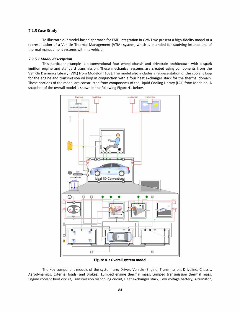
84

7.2.5 Case Study

To illustrate our model-based approach for FMU integration in C2WT we present a high-fidelity model of a representation of a Vehicle Thermal Management (VTM) system, which is intended for studying interactions of thermal management systems within a vehicle.

7.2.5.1 Model description

This particular example is a conventional four wheel chassis and drivetrain architecture with a spark ignition engine and standard transmission. These mechanical systems are created using components from the Vehicle Dynamics Library (VDL) from Modelon [103]. The model also includes a representation of the coolant loop for the engine and transmission oil loop in conjunction with a four heat exchanger stack for the thermal domain. These portions of the model are constructed from components of the Liquid Cooling Library (LCL) from Modelon. A snapshot of the overall model is shown in the following Figure 41 below.

Figure 41: Overall system model

The key component models of the system are: Driver, Vehicle (Engine, Transmission, Driveline, Chassis,

Aerodynamics, External loads, and Brakes), Lumped engine thermal mass, Lumped transmission thermal mass, Engine coolant fluid circuit, Transmission oil cooling circuit, Heat exchanger stack, Low voltage battery, Alternator,

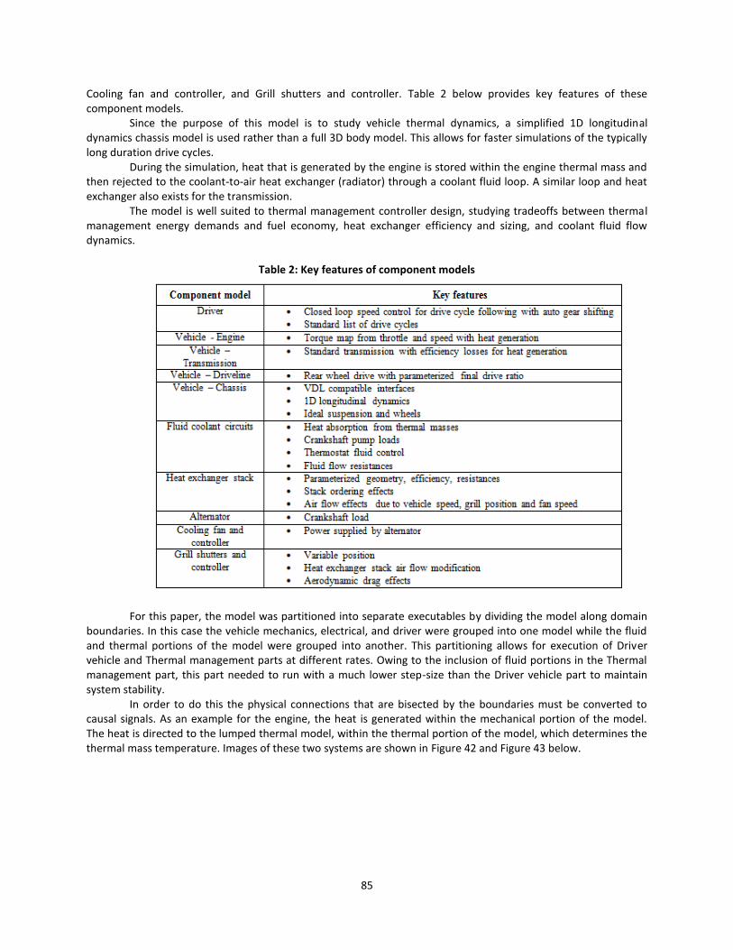
85

Cooling fan and controller, and Grill shutters and controller. Table 2 below provides key features of these component models.

Since the purpose of this model is to study vehicle thermal dynamics, a simplified 1D longitudinal dynamics chassis model is used rather than a full 3D body model. This allows for faster simulations of the typically long duration drive cycles.

During the simulation, heat that is generated by the engine is stored within the engine thermal mass and then rejected to the coolant-to-air heat exchanger (radiator) through a coolant fluid loop. A similar loop and heat exchanger also exists for the transmission.

The model is well suited to thermal management controller design, studying tradeoffs between thermal management energy demands and fuel economy, heat exchanger efficiency and sizing, and coolant fluid flow dynamics.

Table 2: Key features of component models

For this paper, the model was partitioned into separate executables by dividing the model along domain

boundaries. In this case the vehicle mechanics, electrical, and driver were grouped into one model while the fluid and thermal portions of the model were grouped into another. This partitioning allows for execution of Driver vehicle and Thermal management parts at different rates. Owing to the inclusion of fluid portions in the Thermal management part, this part needed to run with a much lower step-size than the Driver vehicle part to maintain system stability.

In order to do this the physical connections that are bisected by the boundaries must be converted to causal signals. As an example for the engine, the heat is generated within the mechanical portion of the model. The heat is directed to the lumped thermal model, within the thermal portion of the model, which determines the thermal mass temperature. Images of these two systems are shown in Figure 42 and Figure 43 below.

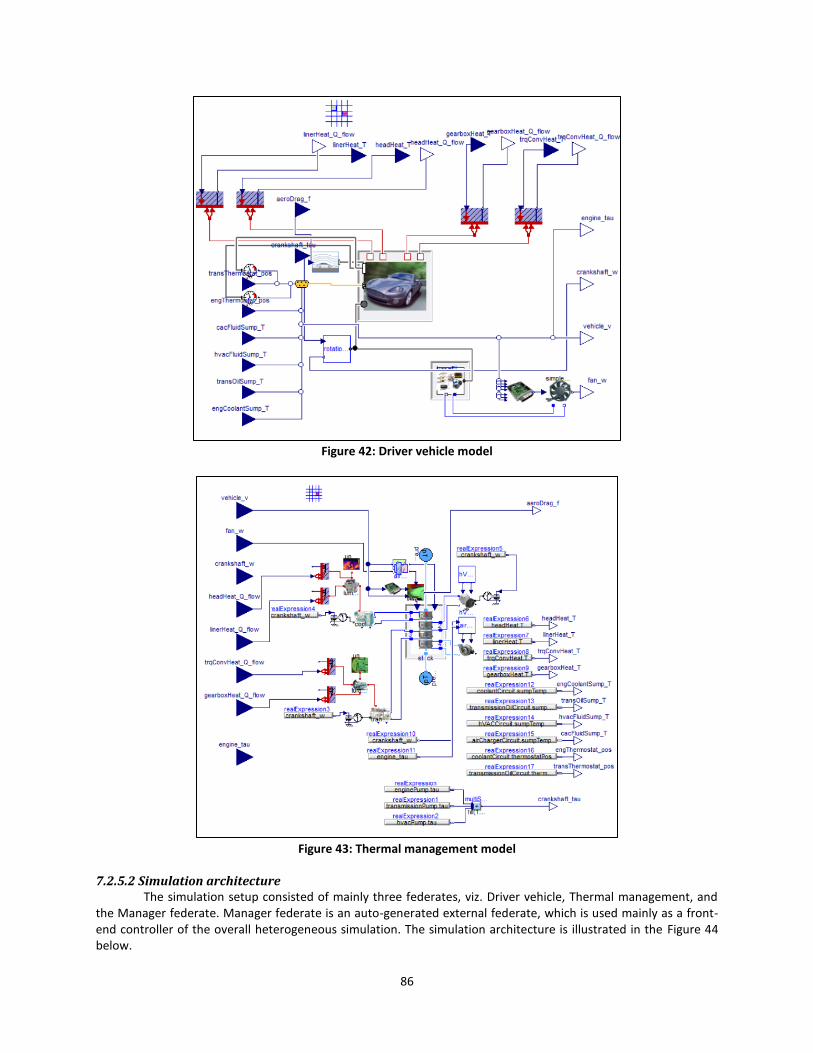
86

Figure 42: Driver vehicle model

Figure 43: Thermal management model

7.2.5.2 Simulation architecture

The simulation setup consisted of mainly three federates, viz. Driver vehicle, Thermal management, and the Manager federate. Manager federate is an auto-generated external federate, which is used mainly as a front-end controller of the overall heterogeneous simulation. The simulation architecture is illustrated in the Figure 44 below.

87

Figure 44: Simulation architecture

7.2.5.3 Data and Integration model

The actual data and integration model are given in the Figure 45 and Figure 46. These show the input and variables from the Driver vehicle and Thermal management federates. These two models are executed as FMUs in the C2WT.

88

Figure 45: Data model

Figure 46: Integration model

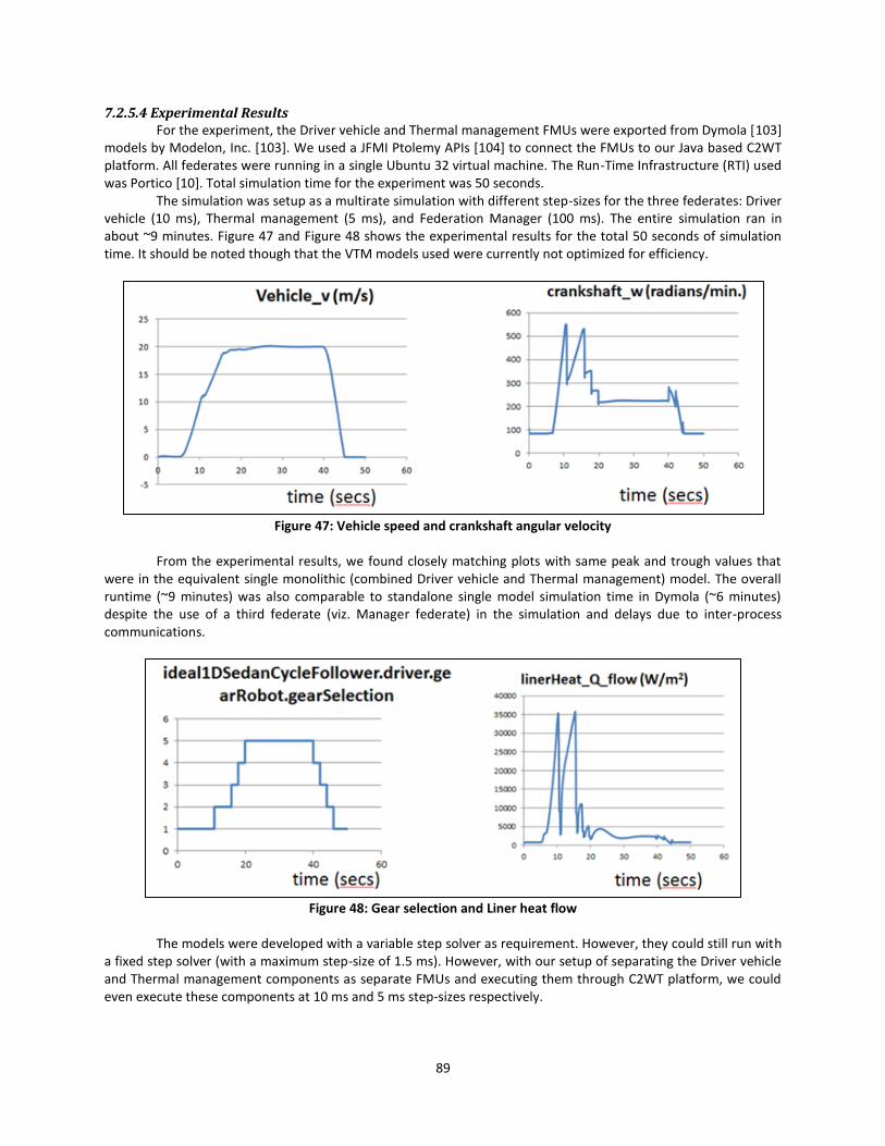
89

7.2.5.4 Experimental Results For the experiment, the Driver vehicle and Thermal management FMUs were exported from Dymola [103]

models by Modelon, Inc. [103]. We used a JFMI Ptolemy APIs [104] to connect the FMUs to our Java based C2WT platform. All federates were running in a single Ubuntu 32 virtual machine. The Run-Time Infrastructure (RTI) used was Portico [10]. Total simulation time for the experiment was 50 seconds.

The simulation was setup as a multirate simulation with different step-sizes for the three federates: Driver vehicle (10 ms), Thermal management (5 ms), and Federation Manager (100 ms). The entire simulation ran in about ~9 minutes. Figure 47 and Figure 48 shows the experimental results for the total 50 seconds of simulation time. It should be noted though that the VTM models used were currently not optimized for efficiency.

Figure 47: Vehicle speed and crankshaft angular velocity

From the experimental results, we found closely matching plots with same peak and trough values that

were in the equivalent single monolithic (combined Driver vehicle and Thermal management) model. The overall runtime (~9 minutes) was also comparable to standalone single model simulation time in Dymola (~6 minutes) despite the use of a third federate (viz. Manager federate) in the simulation and delays due to inter-process communications.

Figure 48: Gear selection and Liner heat flow

The models were developed with a variable step solver as requirement. However, they could still run with

a fixed step solver (with a maximum step-size of 1.5 ms). However, with our setup of separating the Driver vehicle and Thermal management components as separate FMUs and executing them through C2WT platform, we could even execute these components at 10 ms and 5 ms step-sizes respectively.

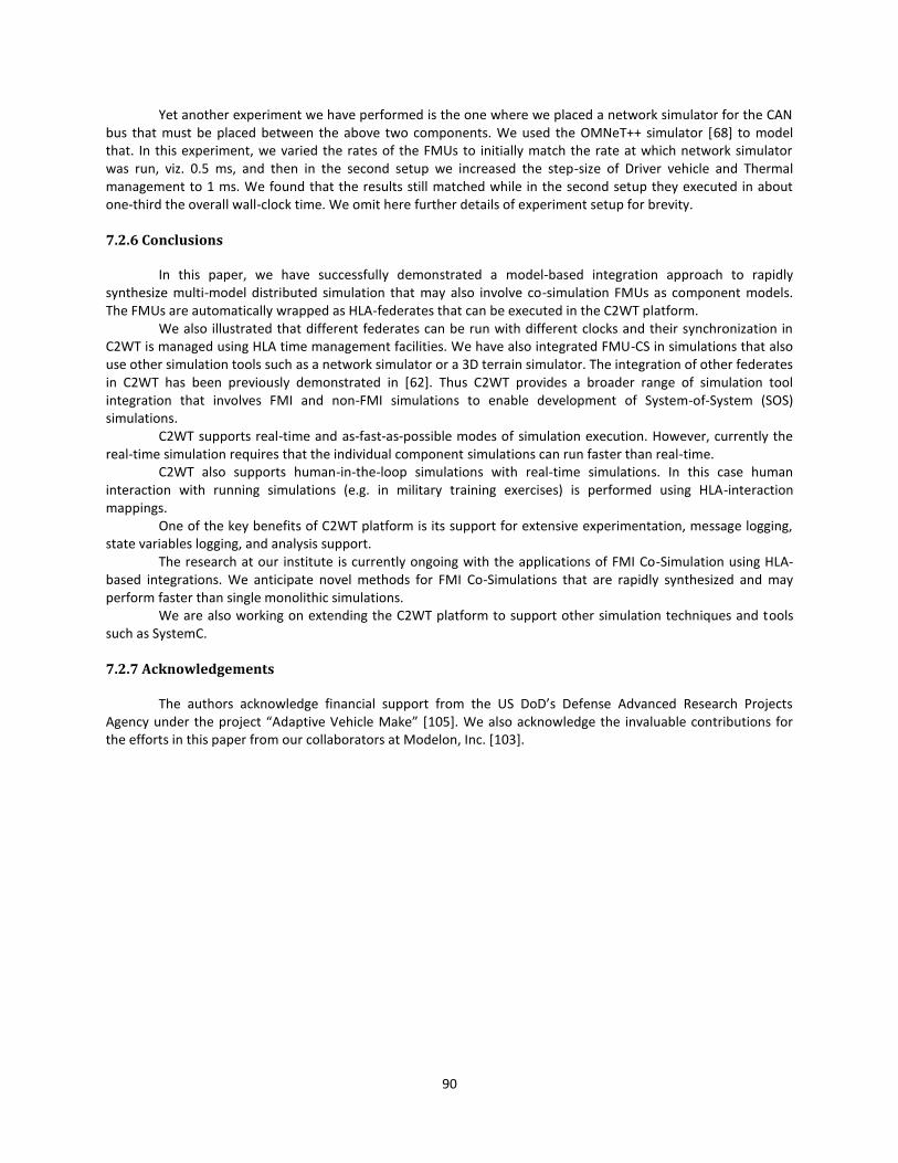
90

Yet another experiment we have performed is the one where we placed a network simulator for the CAN bus that must be placed between the above two components. We used the OMNeT++ simulator [68] to model that. In this experiment, we varied the rates of the FMUs to initially match the rate at which network simulator was run, viz. 0.5 ms, and then in the second setup we increased the step-size of Driver vehicle and Thermal management to 1 ms. We found that the results still matched while in the second setup they executed in about one-third the overall wall-clock time. We omit here further details of experiment setup for brevity.

7.2.6 Conclusions

In this paper, we have successfully demonstrated a model-based integration approach to rapidly synthesize multi-model distributed simulation that may also involve co-simulation FMUs as component models. The FMUs are automatically wrapped as HLA-federates that can be executed in the C2WT platform.

We also illustrated that different federates can be run with different clocks and their synchronization in C2WT is managed using HLA time management facilities. We have also integrated FMU-CS in simulations that also use other simulation tools such as a network simulator or a 3D terrain simulator. The integration of other federates in C2WT has been previously demonstrated in [62]. Thus C2WT provides a broader range of simulation tool integration that involves FMI and non-FMI simulations to enable development of System-of-System (SOS) simulations.

C2WT supports real-time and as-fast-as-possible modes of simulation execution. However, currently the real-time simulation requires that the individual component simulations can run faster than real-time.

C2WT also supports human-in-the-loop simulations with real-time simulations. In this case human interaction with running simulations (e.g. in military training exercises) is performed using HLA-interaction mappings.

One of the key benefits of C2WT platform is its support for extensive experimentation, message logging, state variables logging, and analysis support.

The research at our institute is currently ongoing with the applications of FMI Co-Simulation using HLA-based integrations. We anticipate novel methods for FMI Co-Simulations that are rapidly synthesized and may perform faster than single monolithic simulations.

We are also working on extending the C2WT platform to support other simulation techniques and tools such as SystemC.

7.2.7 Acknowledgements

The authors acknowledge financial support from the US DoD’s Defense Advanced Research Projects Agency under the project “Adaptive Vehicle Make” [105]. We also acknowledge the invaluable contributions for the efforts in this paper from our collaborators at Modelon, Inc. [103].

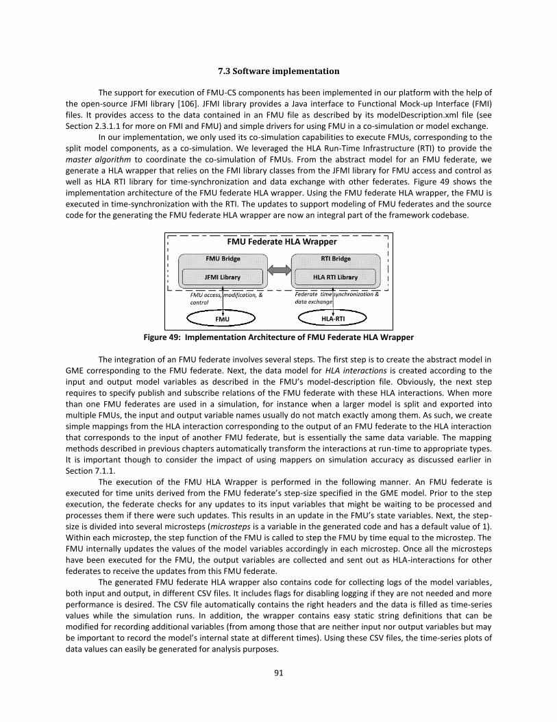
91

7.3 Software implementation

The support for execution of FMU-CS components has been implemented in our platform with the help of the open-source JFMI library [106]. JFMI library provides a Java interface to Functional Mock-up Interface (FMI) files. It provides access to the data contained in an FMU file as described by its modelDescription.xml file (see Section 2.3.1.1 for more on FMI and FMU) and simple drivers for using FMU in a co-simulation or model exchange.

In our implementation, we only used its co-simulation capabilities to execute FMUs, corresponding to the split model components, as a co-simulation. We leveraged the HLA Run-Time Infrastructure (RTI) to provide the master algorithm to coordinate the co-simulation of FMUs. From the abstract model for an FMU federate, we generate a HLA wrapper that relies on the FMI library classes from the JFMI library for FMU access and control as well as HLA RTI library for time-synchronization and data exchange with other federates. Figure 49 shows the implementation architecture of the FMU federate HLA wrapper. Using the FMU federate HLA wrapper, the FMU is executed in time-synchronization with the RTI. The updates to support modeling of FMU federates and the source code for the generating the FMU federate HLA wrapper are now an integral part of the framework codebase.

Figure 49: Implementation Architecture of FMU Federate HLA Wrapper

The integration of an FMU federate involves several steps. The first step is to create the abstract model in

GME corresponding to the FMU federate. Next, the data model for HLA interactions is created according to the input and output model variables as described in the FMU’s model-description file. Obviously, the next step requires to specify publish and subscribe relations of the FMU federate with these HLA interactions. When more than one FMU federates are used in a simulation, for instance when a larger model is split and exported into multiple FMUs, the input and output variable names usually do not match exactly among them. As such, we create simple mappings from the HLA interaction corresponding to the output of an FMU federate to the HLA interaction that corresponds to the input of another FMU federate, but is essentially the same data variable. The mapping methods described in previous chapters automatically transform the interactions at run-time to appropriate types. It is important though to consider the impact of using mappers on simulation accuracy as discussed earlier in Section 7.1.1.

The execution of the FMU HLA Wrapper is performed in the following manner. An FMU federate is executed for time units derived from the FMU federate’s step-size specified in the GME model. Prior to the step execution, the federate checks for any updates to its input variables that might be waiting to be processed and processes them if there were such updates. This results in an update in the FMU’s state variables. Next, the step-size is divided into several microsteps (microsteps is a variable in the generated code and has a default value of 1). Within each microstep, the step function of the FMU is called to step the FMU by time equal to the microstep. The FMU internally updates the values of the model variables accordingly in each microstep. Once all the microsteps have been executed for the FMU, the output variables are collected and sent out as HLA-interactions for other federates to receive the updates from this FMU federate.

The generated FMU federate HLA wrapper also contains code for collecting logs of the model variables, both input and output, in different CSV files. It includes flags for disabling logging if they are not needed and more performance is desired. The CSV file automatically contains the right headers and the data is filled as time-series values while the simulation runs. In addition, the wrapper contains easy static string definitions that can be modified for recording additional variables (from among those that are neither input nor output variables but may be important to record the model’s internal state at different times). Using these CSV files, the time-series plots of data values can easily be generated for analysis purposes.

92

7.4 Guidelines for systematic partitioning and tuning of models

Partitioning a model into sub-component models is useful in three distinct use-cases: 1. When there are external simulation federates that depend, for inputs and outputs, on only a few sub-

components of the overall model. For example, an external federate that needs to record high frequency data on engine speed in order to evaluate the operator’s driving habits. In this case, it is sub-optimal to pause the entire model of the engine/car at every few microseconds in order to output the current engine speed to the external federate. As such, it is performance-wise beneficial to split the model such that only the component outputting the engine speed is scaled down to few microseconds step-size and the rest of the model could be executed faster at much larger step-size.

2. The second use-case is when the model is so large that it is prohibitively expensive to execute on a single compute node. In this case, it is desirable to split the model into sub-component models and execute them as separate FMU federates on different compute nodes.

3. The third use-case is the one in which there are parts in a large model that are known to require a much smaller step-size in order to be executed in a stable manner (as illustrated in section 7.2). In this case, the parts that require a small step-size in order to remain stable become a bottleneck on the performance of the entire model because when the entire model is executed as a whole, that step-size becomes the maximum allowable. Thus, to increase overall performance the model can be split such that the parts that require much small step-sizes are separated as different FMU federates than the rest of the model. Once the model split is determined according to one of the use-cases above, one needs careful evaluation

of the split models for stability and performance. The goal is to maximize the step-sizes that can be achieved while still keeping the model execution stable. Below we describe a simple procedure for arriving at the maximal step-sizes of the split models. This is the method we also used in tuning the use-case described in the paper in section 7.2. For the procedure below, let the part exhibiting fast dynamics (thus requiring a smaller step-size) be P_f, and the part exhibiting relatively slow dynamics (thus executes in a stable manner even with a comparatively much large step-size) be P_s. Let the maximum step-size at which the single overall model executes in a stable manner be SS_combined. It is assumed that the original model, before being partitioned, was already optimized to run as efficiently as possible, which resulted in executing it with the maximum step-size possible, viz. SS_combined.

1. Set the step-size of P_f and P_s to SS_combined. For the most cases, as the original model could run stable with step-size as much as SS_combined (i.e., decreasing the step-size from SS_combined will not be needed), this will still lead to a stable execution across split sub-component models. In this step and the ones below, we check the stability of the model execution by comparing the values of model variables through time between the original single model and the split sub-component models.

2. Next, we increase the step-size of P_f in small increments while still making sure that execution of split sub-component models is still stable.

3. Next, we increase the step-size of P_s in small increments, while still making sure that execution of split sub-component models is still stable.

4. We repeat steps 2 and 3 successively to arrive at the maximum step-sizes that still keep the model execution stable and, at the same time, the values of the model variables are within the acceptable limits as compared to the values obtained when the entire model was executed as a whole. We stop when step-size could not be increased in any of the above two steps.

7.5 Summary

Large dynamical models often have many sub-component models that exhibit different rate dynamics. This effectively means that some parts of the models could be executed much faster (i.e., take less computation time on average per step) than the others. These models could be more efficiently executed if they are split across sampling rate boundaries. In this chapter, we provided our solution to enable such partitioning of the model using the FMI standard for packaging the split models and executing them together as HLA federates. We also described a fully automated framework for modeling and execution of the split models. Further, we provided guidelines for systematically partitioning the models and tuning their step-sizes to achieve the maximum performance. For more than two partitions, similar tuning can be done by going from partitions with fastest to slowest rate dynamics.

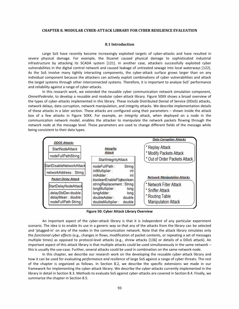
93

CHAPTER 8. MODULAR CYBER-ATTACK LIBRARY FOR CYBER RESILIENCE EVALUATION

8.1 Introduction

Large SoS have recently become increasingly exploited targets of cyber-attacks and have resulted in severe physical damage. For example, the Stuxnet caused physical damage to sophisticated industrial infrastructure by attacking its SCADA system [121]. In another case, attackers successfully exploited cyber vulnerabilities in the digital control network and caused leakage of untreated sewage into local waterways [122]. As the SoS involve many tightly interacting components, the cyber-attack surface grows larger than on any individual component because the attackers can actively exploit combinations of cyber vulnerabilities and attack the target systems through other interconnected systems. Therefore, it is important to analyze SoS’ performance and reliability against a range of cyber-attacks.

In this research work, we extended the reusable cyber communication network simulation component, OmnetFederate, to develop a reusable and modular cyber-attack library. Figure 50XX shows a broad overview of the types of cyber-attacks implemented in this library. These include Distributed Denial of Service (DDoS) attacks, network delays, data corruption, network manipulation, and integrity attacks. We describe implementation details of these attacks in a later section. These attacks are configured using their parameters – shown inside the attack box of a few attacks in Figure 50XX. For example, an integrity attack, when deployed on a node in the communication network model, enables the attacker to manipulate the network packets flowing through the network node at the message level. These parameters are used to change different fields of the message while being consistent to their data types.

Figure 50: Cyber Attack Library Overview

An important aspect of the cyber-attack library is that it is independent of any particular experiment

scenario. The idea is to enable its use in a generic way so that any of the attacks from the library can be selected and ‘plugged-in’ on any of the nodes in the communication network. Note that the attack library simulates only the functional cyber effects (e.g., changes in flows, modification of packet contents, or repeating a set of messages multiple times) as opposed to protocol-level attacks (e.g., shrew attacks [136] or details of a DDoS attack). An important aspect of this attack library is that multiple attacks could be used simultaneously in the same network – this is usually the use-case. Further, several attacks could be used in combination on the same network node.

In this chapter, we describe our research work on the developing the reusable cyber-attack library and how it can be used for evaluating performance and resilience of large SoS against a range of cyber threats. The rest of the chapter is organized as follows. In Section 8.2, we describe the specific extensions we made in our framework for implementing the cyber-attack library. We describe the cyber-attacks currently implemented in the library in detail in Section 8.3. Methods to evaluate SoS against cyber-attacks are covered in Section 8.4. Finally, we summarize the chapter in Section 8.5.

94

8.2 Framework Extensions for Implementing the Cyber-Attack Library

Previously, in Section 6.3, we described how OMNeT++ modules could be customized to create a reusable OmnetFederate that can be repurposed for different network topologies used in different experiment scenarios. In this section, we describe additional extensions we made to create the reusable cyber-attack library.

First, we heavily customized the UDP basic module to add parameters specific to all of the cyber-attacks that needed to be handled in the application layer. For example, to support an integrity attack, we added parameters to capture the modifications on different data types supported for variations in a message. For example, for ‘integer’ fields of a message, we added two parameters, viz. ‘intMultipler’ and ‘intAdder’. The outgoing message after the integrity attack will have the integer fields modified by first multiplying it by the value of ‘intMultiplier’ and then adding the value of ‘intAdder’ to it. Similarly, message fields with other data types such as long, double, Boolean, and string, required additional parameters to allow tweaking the value of those fields in a configurable manner.

The integrity attack modifies the incoming HLA interactions using the parameters of the attack. It is configured for modifying network interactions, which pass through the simulated network, according to the values of parameters specified while configuring the attack. The receiver federate of the HLA interaction receives a slightly modified version of parameter values as compared to the ones in the interaction that was originally sent by the sender federate. It is important to note that the integrity attack is a special attack that works on domain-specific HLA interactions that are not known in advance. Therefore, to implement configuration and handling of this attack in a generic manner in the reusable cyber-attack library, we use static code segments that include definitions of scenario-specific interactions. The static code segments are loaded before the main program executes, thus ensuring that all static initialization in the C++ classes corresponding to these scenario-specific interactions are performed prior to running the main program. In addition, we use the generated classes to figure out the maps of interaction parameters and their data types so that we could manipulate them at run-time and package the updated values as a new modified HLA interaction. This is needed because OmnetFederate communicates using only a pre-defined interaction type, viz. NetworkPacket, and the actual content of the message must be inferenced from the interaction’s string formatted field called ‘data’. The value of the data field is modified according to the attack configuration, and then repackaged into a new interaction.

Secondly, several attacks, such as sniffer and packet delay attacks, in the library required manipulating the packet transmission at the IP layer within the stack of network layers. Another example of an attack implemented in the IP layer is the network filter attack. To implement it, we need to ensure that all network traffic between two given subnets must be filtered out (i.e., dropped), while letting through the rest of the network communications. In order to implement the network filter attack, we extended the IP module of the INET Framework in OMNeT++ in the same way to parameterize it for the configuration of attack and to handle the attack at run-time. When a network packet flows through the network stack, it eventually crosses the IP layer. Here, if the host has the network filter attack configured, before letting the transmission of the packet through regular channels, it is matched against the source and destination subnets specified in the network filter attack. If both the source and destination subnet addresses match, the packet is dropped, and a log is generated for the dropped packet.

Thirdly, we created message definitions for all the cyber-attacks in the library. These definitions include the parameters to configure the attacks. These message definitions are automatically translated to C++ classes by OMNeT++ at compile time. These messages are used to configure the attacks on the network nodes at run-time. The reader is referred to Appendix B for sample code listings that show how the above cyber-attacks were implemented in C++.

Finally, we defined HLA interactions in the data-model of OmnetFederate and implemented handlers in the HLAInterface module to handle turning the cyber-attacks ON and OFF at run-time depending on which interactions are received (corresponding to the starting or stopping the cyber-attack). These handlers use the parameter values of the attacks to configure their behavior accordingly. Using these handlers one can ‘plug-in’ many different cyber-attacks from the library at many different network nodes dynamically during the run-time.

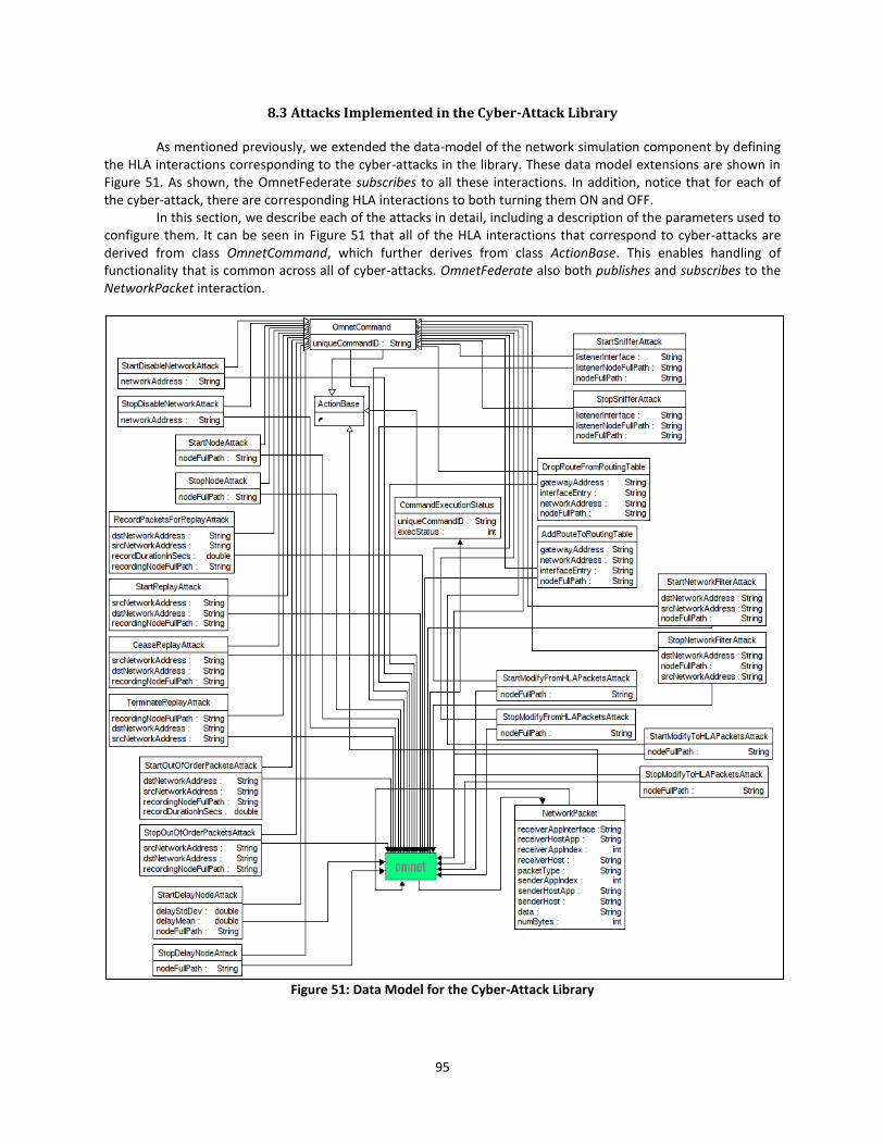
95

8.3 Attacks Implemented in the Cyber-Attack Library

As mentioned previously, we extended the data-model of the network simulation component by defining the HLA interactions corresponding to the cyber-attacks in the library. These data model extensions are shown in Figure 51. As shown, the OmnetFederate subscribes to all these interactions. In addition, notice that for each of the cyber-attack, there are corresponding HLA interactions to both turning them ON and OFF.

In this section, we describe each of the attacks in detail, including a description of the parameters used to configure them. It can be seen in Figure 51 that all of the HLA interactions that correspond to cyber-attacks are derived from class OmnetCommand, which further derives from class ActionBase. This enables handling of functionality that is common across all of cyber-attacks. OmnetFederate also both publishes and subscribes to the NetworkPacket interaction.

Figure 51: Data Model for the Cyber-Attack Library

96

Next, we list the various cyber-attacks in the cyber-attack library and discuss how each of them work and affect the network simulation.

For describing the cyber-attacks, we will use the following terms in the descriptions: 1. node: A node can be a host computer, a switch, or a router. 2. link: A link is a direct connection between two nodes. Thus, a link can be a specific connection between a

router and a switch. 3. network: A network is a graph of interconnected network elements such as hosts, switches, and routers.

It may be the entire network in the simulation, or any part of it. Following are the cyber-attacks in the cyber-attack library (see Appendix E for a detailed discussion of

these cyber-attacks, their behavior, parameters used to configure them, and their current implementation status): 1. DOS Attack: Completely disable a specific node on the network. This essentially means that the node

stops functioning for the duration of simulation causing all packets routed to it or going to be generated by it to be dropped.

2. Disable and Degrade Network Attack: Changes the behavior of the network such that the network packets that go through the network are either dropped, or delayed, or congested, or they incur losses.

3. Network Filter Attack: Filter (i.e. drop) transmission of packets flowing between a given network address to another network address via a given node.

4. Disrupt Link Attack: Changes the behavior of a specific network link. 5. Replay Attack: A malicious node (usually a router) intercepts and buffers packets for a given duration and

when activated, it ‘replays’ them in order until the attack is ceased or terminated. 6. Packet Modification Attack: The attacker intercepts, inspects, modifies, and then sends out the modified

network packets. 7. Data Injection Attack: Injects a new network packet into a specific link in the network. 8. Out-of-order Packets Attack: A malicious node in the network buffers and re-sequences network packets.

This means that sending order will be different from the receiving order. When the attack is launched, the node records the packets for the given duration periodically (period = record duration) and replays them in a random order.

9. Sniffer Attack: A node relays all messages going through it to another listener host. 10. Masquerading Attack: A malicious host masquerades as another, legal host. All packets are intercepted

by the malicious host and are responded. The legal host does not see anything from the intercepted traffic.

11. DNS Poisoning Attack: An entry in the Domain Name Service (DNS) host is modified, such that lookups of ‘affected’ host results in the address of the ‘attacker’ host, causing all subsequent traffic meant for the affected host to be relayed to the attacker host.

12. Routing Table Modification Attack: Change an entry in the routing tables of a node (usually a router), causing network packets to be misrouted.

13. Delay Node Attack: Delay packets that flow along the malicious node in the network. This can be used to slowdown certain routers, switches, or hosts, in the network such that all communications along a specific network path is delayed.

14. Delay Path Attack: Delay flow of packets along a path in the network. This can be used for communication delay along a specific path in the network.

8.4 Evaluating SoS Against Cyber-Attacks

In order to evaluate large SoS against cyber threats, we need to run several experiments with different combinations of cyber-attacks. In our framework, we use the Federation Manager component to inject HLA interactions that turn the cyber-attacks ON or OFF. The reader is referred to Section 4.5.2, where we described the features of the Federation Manager, including how it can be configured to send interactions into the running simulation at run-time. Essentially, this requires one to change the configuration XML file for the Federation Manager to include the interactions to be injected at run-time, along with the time of the injection and values of all the parameters of the interaction.

97

The capability to conduct distributed simulation experiments of large SoSs along with the use different combinations of cyber-attacks from the cyber-attack library allows the evaluation of the resilience of the entire SoS. In other words, it allows studying the reaction of the entire SoS (with all its simulated applications and components) when under various cyber-attacks. Note that this is beyond evaluating low-level cybersecurity measures (which may or may not be effective).

The defense against cyber threats is usually achievable through several security mechanisms. For example, unauthorized users can be prevented from network access through encryption techniques or IP firewalls on network entry points. In our framework, we developed methods to automatically compose combinations of cyber-attacks and defense mechanisms and execute corresponding experiments in batch mode (i.e., sequentially without manual intervention). The main idea is to be able to configure such permutations of evaluation scenarios rapidly so that, when they are executed in an automated manner, a full set of analysis results can be generated. We accomplish this by allowing configuration of injected interactions in experiment models. For a particular evaluation scenario of a SoS, many experiment models with different combination of injected interactions can be created and all combinations can be evaluated in a batch mode automatically. The results of all different execution runs of the experiments are recorded in log files and in a central MySQL database. The results can then be post-processed for further analysis after all experiments have finished execution.

8.5 Summary

Owing to their interconnected and interdependent nature, large SoS have become increasingly a target of cyber-attacks, requiring their thorough evaluations against such cyber threats. The communication network is central to all systems in the SoS and enables cyber-attacks to affect the target system in indirect ways.

In this chapter, we described our work on developing a reusable and modular cyber-attack library that allows experimenters to 'plug-in' many different cyber-attacks at different time-points and network nodes in the SoS simulations. In this library, we developed models for a number of cyber-attacks that are useful for evaluating SoS's performance and reliability such as Distributed Denial of Service (DDoS) attacks, network delays, data corruption, network manipulation, and integrity attacks. It is important to note that, at the SoS level, similar impacts on the network performance can be achieved through variety of cyber-attacks. For example, a timeout in the receiving messages can be achieved by attacking the receiver node, disabling part of the network where the receiver node lies, delaying the packets, and using a network filter attack along the path to the receiver node. The cyber-attack library is domain-independent and it is up to the experimenters to choose the set of cyber-attacks to deploy as test conditions in their experiments. In addition, experimenters often need to evaluate SoS against several what-if scenarios that need a detailed workflow to be programmed for evaluations (we defined this previously as scenario-based experimentation in Section 2.2.2.3). We will describe the methods and tools we developed for scenario-based experimentation in detail in Chapter 9.

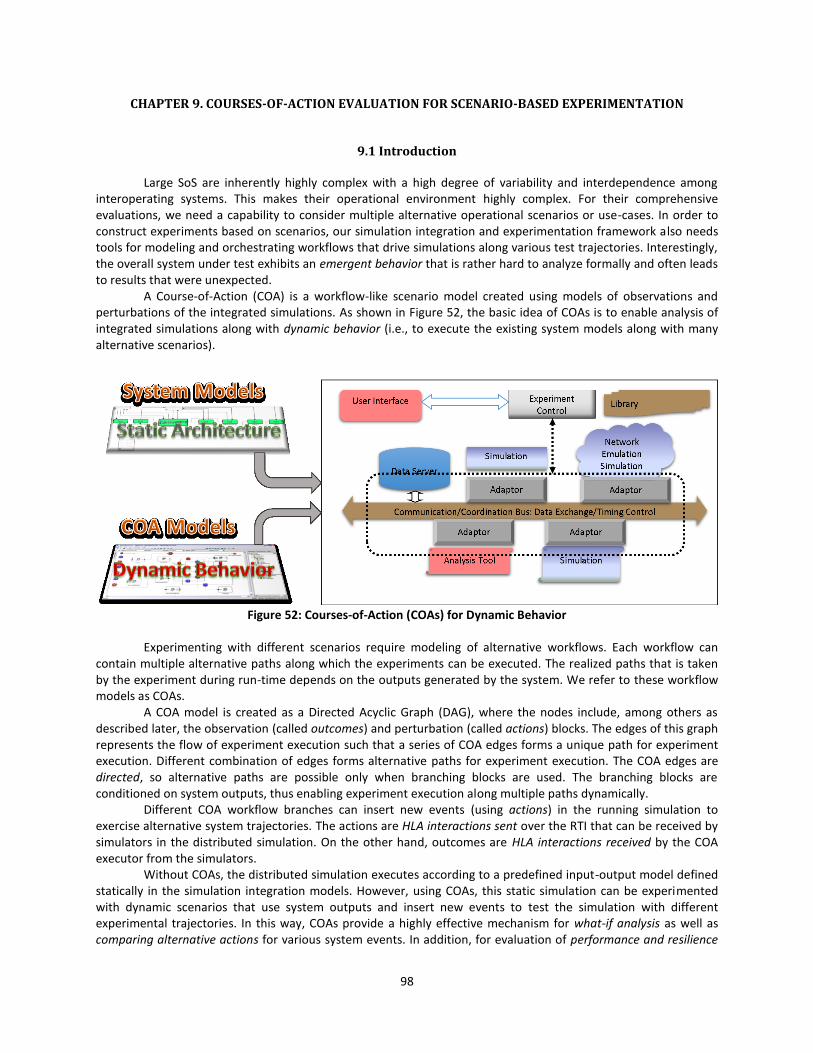
98

CHAPTER 9. COURSES-OF-ACTION EVALUATION FOR SCENARIO-BASED EXPERIMENTATION

9.1 Introduction

Large SoS are inherently highly complex with a high degree of variability and interdependence among interoperating systems. This makes their operational environment highly complex. For their comprehensive evaluations, we need a capability to consider multiple alternative operational scenarios or use-cases. In order to construct experiments based on scenarios, our simulation integration and experimentation framework also needs tools for modeling and orchestrating workflows that drive simulations along various test trajectories. Interestingly, the overall system under test exhibits an emergent behavior that is rather hard to analyze formally and often leads to results that were unexpected.

A Course-of-Action (COA) is a workflow-like scenario model created using models of observations and perturbations of the integrated simulations. As shown in Figure 52, the basic idea of COAs is to enable analysis of integrated simulations along with dynamic behavior (i.e., to execute the existing system models along with many alternative scenarios).

Figure 52: Courses-of-Action (COAs) for Dynamic Behavior

Experimenting with different scenarios require modeling of alternative workflows. Each workflow can

contain multiple alternative paths along which the experiments can be executed. The realized paths that is taken by the experiment during run-time depends on the outputs generated by the system. We refer to these workflow models as COAs.

A COA model is created as a Directed Acyclic Graph (DAG), where the nodes include, among others as described later, the observation (called outcomes) and perturbation (called actions) blocks. The edges of this graph represents the flow of experiment execution such that a series of COA edges forms a unique path for experiment execution. Different combination of edges forms alternative paths for experiment execution. The COA edges are directed, so alternative paths are possible only when branching blocks are used. The branching blocks are conditioned on system outputs, thus enabling experiment execution along multiple paths dynamically.

Different COA workflow branches can insert new events (using actions) in the running simulation to exercise alternative system trajectories. The actions are HLA interactions sent over the RTI that can be received by simulators in the distributed simulation. On the other hand, outcomes are HLA interactions received by the COA executor from the simulators.

Without COAs, the distributed simulation executes according to a predefined input-output model defined statically in the simulation integration models. However, using COAs, this static simulation can be experimented with dynamic scenarios that use system outputs and insert new events to test the simulation with different experimental trajectories. In this way, COAs provide a highly effective mechanism for what-if analysis as well as comparing alternative actions for various system events. In addition, for evaluation of performance and resilience

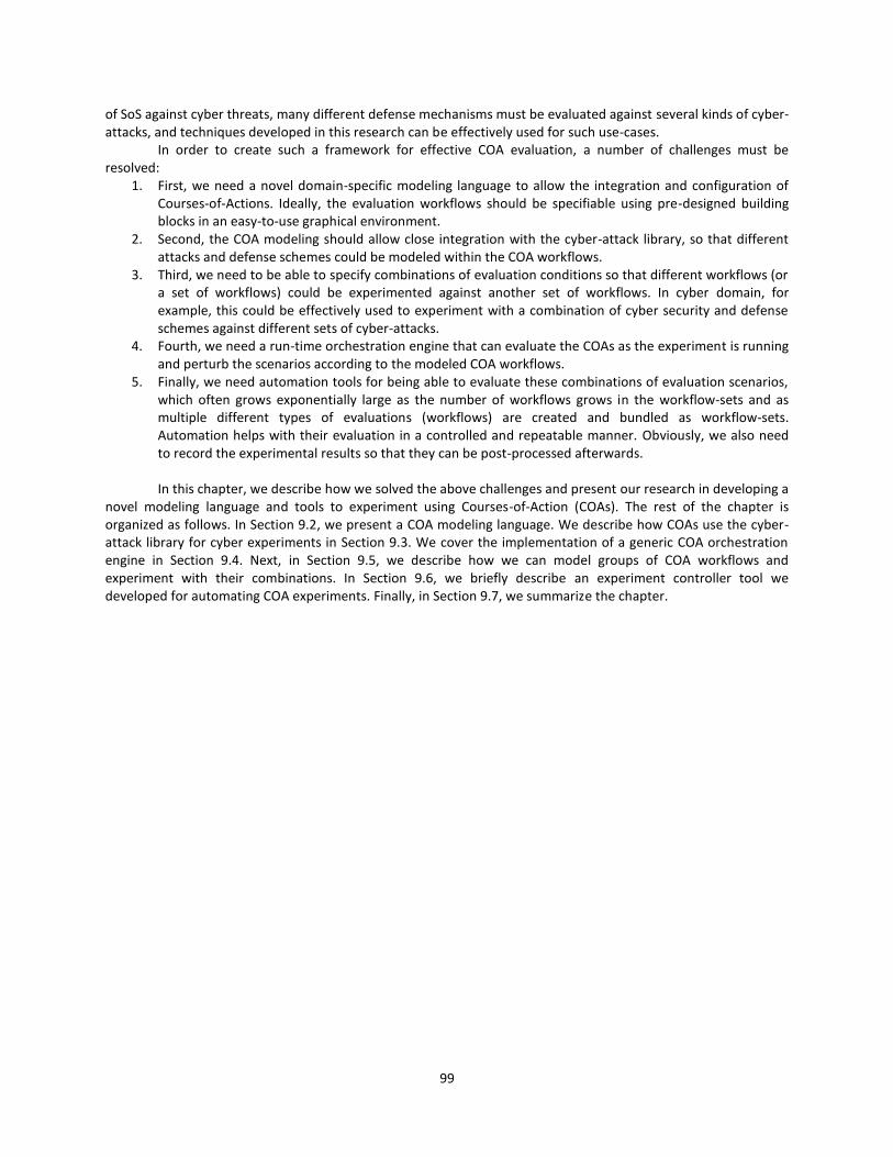
99

of SoS against cyber threats, many different defense mechanisms must be evaluated against several kinds of cyber-attacks, and techniques developed in this research can be effectively used for such use-cases.

In order to create such a framework for effective COA evaluation, a number of challenges must be resolved:

1. First, we need a novel domain-specific modeling language to allow the integration and configuration of Courses-of-Actions. Ideally, the evaluation workflows should be specifiable using pre-designed building blocks in an easy-to-use graphical environment.

2. Second, the COA modeling should allow close integration with the cyber-attack library, so that different attacks and defense schemes could be modeled within the COA workflows.

3. Third, we need to be able to specify combinations of evaluation conditions so that different workflows (or a set of workflows) could be experimented against another set of workflows. In cyber domain, for example, this could be effectively used to experiment with a combination of cyber security and defense schemes against different sets of cyber-attacks.

4. Fourth, we need a run-time orchestration engine that can evaluate the COAs as the experiment is running and perturb the scenarios according to the modeled COA workflows.

5. Finally, we need automation tools for being able to evaluate these combinations of evaluation scenarios, which often grows exponentially large as the number of workflows grows in the workflow-sets and as multiple different types of evaluations (workflows) are created and bundled as workflow-sets. Automation helps with their evaluation in a controlled and repeatable manner. Obviously, we also need to record the experimental results so that they can be post-processed afterwards. In this chapter, we describe how we solved the above challenges and present our research in developing a

novel modeling language and tools to experiment using Courses-of-Action (COAs). The rest of the chapter is organized as follows. In Section 9.2, we present a COA modeling language. We describe how COAs use the cyber-attack library for cyber experiments in Section 9.3. We cover the implementation of a generic COA orchestration engine in Section 9.4. Next, in Section 9.5, we describe how we can model groups of COA workflows and experiment with their combinations. In Section 9.6, we briefly describe an experiment controller tool we developed for automating COA experiments. Finally, in Section 9.7, we summarize the chapter.

100

9.2 COA Modeling Language

In our framework, we extended the core metamodel to support modeling of COAs. The key additions are: (1) the atomic building blocks that can be composed together to create COAs and (2) COA groups that can be used to package multiple COAs as workflow-sets and experimented with their combinations. Figure 53 shows a simplified version of the part of metamodel we developed for COA modeling. As shown, we defined a number of individual atomic blocks that are used to create COAs. We call these atomic blocks as ‘COA elements’ and these include synchronization point, action, outcome, fork, probabilistic choice, awaitN, duration, random duration, outcome filter, and terminate COA. We describe the semantics of each of these COA elements next.

An important point to note is that the COA elements action and outcome have been created as References and they refer to a HLA interaction. This allows using actions and outcomes to specify the injection and observation of the referred HLA interactions. Table 3 lists all of the above-mentioned COA elements along with a detailed description of their semantics. Note that these COA elements are similar to those used in a workflow model in the Business Process Modeling Notation (BPMN) [123] and even uses similar icons. BPMN uses elements like events, activities, and gateways (with several variations of each) and flows to connect them into creating business workflows. In BPMN, events denote something that happens in the workflow, activities denote a task or work that is done, and gateways denote forking and merging points in the workflow. In our COA language, BPMN events are analogous to outcomes, which represent HLA interactions generated by simulators and received by the COA executor; BPMN activities are analogous to actions, which represent HLA interactions injected (sent) by the COA executor; and BPMN gateways have corresponding variations such forks, awaitN, and probabilisticChoice. Elements in our COA language are designed for HLA-based simulations and include many other types for fully supporting SoS COA models as described in Table 3.

Figure 53: COA Modeling Language

101

Table 3: Semantics of COA Elements

COA Element Icon Description

Synchronization Point (and

Exceptions/ timeouts)

This represents the absolute time-point from the beginning of the simulation. The semantics is that all incoming branches must wait until the time-point represented by the synchronization point has been reached. If all incoming branches have been finished, the succeeding success branch is taken. In addition, depending on the number of incoming branches that have finished until the synchronization point, the exception branches can be taken according to the model. For example, in Figure 54 at synchronization point (t=2hrs), if both the branches have succeeded, then the branch with synchronization point (t=3hrs) is activated, otherwise Exception1 branch is triggered.

Action

An action node specifies an interaction that must be sent out by the COA Sequence Executor as soon as the action point is reached in the COA sequence execution. The parameters of the interactions can be specified.

Outcome

An outcome represents the type of an interaction that the COA sequence executor must wait for to arrive before it can proceed. For example, this can represent a planned or expected activity in a scenario that when occurs, an interaction of this type is sent to HLA.

Fork

A Fork element is a branching element. Its semantics are that all branches following a fork element are executed in parallel as soon as the fork element is reached.

Probabilistic Choice

A Probabilistic Choice element chooses only a single succeeding branch. Different branches have a probability specified for their selection. The probabilities of all branches are normalized to 1 if they already do not add to 1. At run-time, a random value between 0 and 1 is chosen and, depending on that value, the appropriate branch is selected for execution.

AwaitN

A simple node that specifies a given number of incoming branches to wait on completing their execution, before letting the COA execution to proceed.

Duration

A duration specifier that represents the time the COA sequence executor delays the execution once the duration element is reached. This time-period is relative to the time when the duration element is reached.

Random Duration

A duration specifier that represents a duration that is randomly distributed using a uniform distribution. For uniform distribution, a range is provided and the orchestrator automatically chooses a value according to a seed value. The seed value can be configured for an experiment for ensuring repeatability of experiments. If no seed is provided, a default value of ‘0’ is used as the seed. Once a value for the random duration is selected, the execution semantics is the same as a regular ‘Duration’ node.

OutcomeFilter

This is an advanced concept and can be used to filter based on the values of the parameters of the received interaction (as an Outcome). Different outgoing branches can be executed based on different values of parameters.

Terminate COA

When reached the COA execution is terminated.

9.3 COA Integration with Cyber-Attack Library

As shown in Chapter 8, in Figure 51, different cyber-attacks are configured through HLA interactions. As the COA element action and outcome are references to HLA interactions, the interactions that turn the cyber-attacks ON or OFF can be used as action and outcome blocks in COA sequence models. Thus, the complex COA workflows can strategically time and place cyber-attacks in them.

Using COAs for deploying cyber-attacks in an experiment is much general and easier to use than the previously described mechanism of using injected interactions directly in Federation Manager (see Section 8.4).

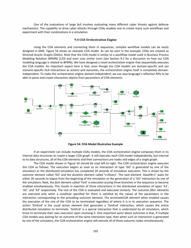
102

One of the evaluations of large SoS involves evaluating many different cyber threats against defense mechanisms. The capability to drive cyber-attacks through COAs enables one to create many such workflows and experiment with their combinations in a simulation.

9.4 COA Orchestration Engine

Using the COA elements and connecting them in sequences, complex workflow models can be easily designed in GME. Figure 54 shows an example COA model. As can be seen in the example, COAs are created as Directed Acyclic Graphs (DAGs). Note that the COA model is similar to a workflow model used in Business Process Modeling Notation (BPMN) [123] and even uses similar icons (see Section 9.2 for a discussion on how our COA modeling language is related to BPMN). We have designed a novel orchestration engine that sequentially executes the COA models. An important aspect here is that, even though the COA models are domain-specific and use scenario-specific HLA interactions as actions and outcomes, the orchestration engine itself is completely domain-independent. To make the orchestration engine domain-independent, we use Java language’s reflection APIs to be able to parse and create interaction objects from parameters of COA elements.

Figure 54: COA Model Illustrative Example

If an experiment can include multiple COAs models, the COA orchestration engine composes them in its

internal data structures to create a larger COA graph. It still executes each COA model independently, but internal to its data structures, all of the COA elements and their connections are nodes and edges of a single graph.

The COA model shown in Figure 54 should be read left-to-right. The COA orchestration engine executes this COA as follows. The execution begins as soon as an interaction of type ‘GO’ is generated by one of the simulators or the distributed simulation has completed 20 seconds of simulation execution. This is shown by the outcome element called ‘GO’ and the duration element called ‘t=20secs’. The next element ‘AwaitN=1’ waits for either 20 seconds to elapse from the beginning of the simulation or the generation of a ‘GO’ interaction by one of the simulators. Next, the fork element called ‘Fork’ is executed causing three branches in the sequence to become enabled simultaneously. This results in injection of three interactions in the distributed simulation of types ‘A1’, ‘A2’, and ‘A3’ respectively. The rest of the COA is evaluated and executed similarly. The outcome filter elements are executed only when a condition specified for them is satisfied by the values of the parameters in the interaction corresponding to the preceding outcome element. The terminateCOA element when enabled causes the execution of the rest of the COA to be terminated regardless of where it is in its execution sequence. The action ‘SimEnd’ is the usual action element that generates a ‘SimEnd’ interaction, which causes the entire distributed simulation to terminate. ‘SimEnd’ is a special interaction that is understood by all simulators, which know to terminate their own execution upon receiving it. One important point about outcomes is that, if multiple COA models was waiting for an outcome of the same interaction type, then when such an interaction is generated by one of the simulators, the COA orchestration engine will execute all of those outcome nodes simultaneously.

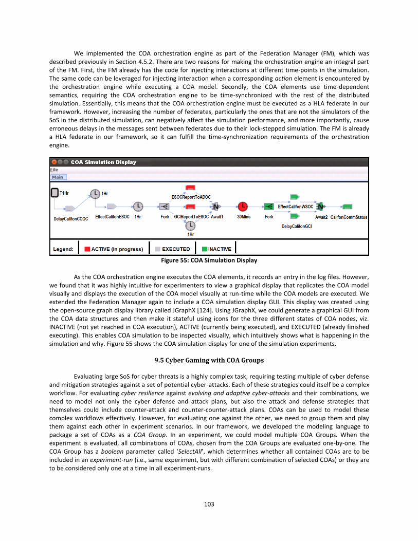
103

We implemented the COA orchestration engine as part of the Federation Manager (FM), which was described previously in Section 4.5.2. There are two reasons for making the orchestration engine an integral part of the FM. First, the FM already has the code for injecting interactions at different time-points in the simulation. The same code can be leveraged for injecting interaction when a corresponding action element is encountered by the orchestration engine while executing a COA model. Secondly, the COA elements use time-dependent semantics, requiring the COA orchestration engine to be time-synchronized with the rest of the distributed simulation. Essentially, this means that the COA orchestration engine must be executed as a HLA federate in our framework. However, increasing the number of federates, particularly the ones that are not the simulators of the SoS in the distributed simulation, can negatively affect the simulation performance, and more importantly, cause erroneous delays in the messages sent between federates due to their lock-stepped simulation. The FM is already a HLA federate in our framework, so it can fulfill the time-synchronization requirements of the orchestration engine.

Figure 55: COA Simulation Display

As the COA orchestration engine executes the COA elements, it records an entry in the log files. However,

we found that it was highly intuitive for experimenters to view a graphical display that replicates the COA model visually and displays the execution of the COA model visually at run-time while the COA models are executed. We extended the Federation Manager again to include a COA simulation display GUI. This display was created using the open-source graph display library called JGraphX [124]. Using JGraphX, we could generate a graphical GUI from the COA data structures and then make it stateful using icons for the three different states of COA nodes, viz. INACTIVE (not yet reached in COA execution), ACTIVE (currently being executed), and EXECUTED (already finished executing). This enables COA simulation to be inspected visually, which intuitively shows what is happening in the simulation and why. Figure 55 shows the COA simulation display for one of the simulation experiments.

9.5 Cyber Gaming with COA Groups

Evaluating large SoS for cyber threats is a highly complex task, requiring testing multiple of cyber defense and mitigation strategies against a set of potential cyber-attacks. Each of these strategies could itself be a complex workflow. For evaluating cyber resilience against evolving and adaptive cyber-attacks and their combinations, we need to model not only the cyber defense and attack plans, but also the attack and defense strategies that themselves could include counter-attack and counter-counter-attack plans. COAs can be used to model these complex workflows effectively. However, for evaluating one against the other, we need to group them and play them against each other in experiment scenarios. In our framework, we developed the modeling language to package a set of COAs as a COA Group. In an experiment, we could model multiple COA Groups. When the experiment is evaluated, all combinations of COAs, chosen from the COA Groups are evaluated one-by-one. The COA Group has a boolean parameter called ‘SelectAll’, which determines whether all contained COAs are to be included in an experiment-run (i.e., same experiment, but with different combination of selected COAs) or they are to be considered only one at a time in all experiment-runs.

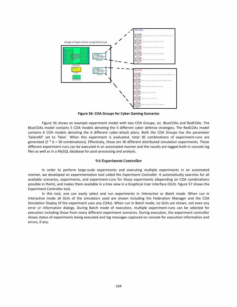
104

Figure 56: COA Groups for Cyber Gaming Scenarios

Figure 56 shows an example experiment model with two COA Groups, viz. BlueCOAs and RedCOAs. The

BlueCOAs model contains 5 COA models denoting the 5 different cyber defense strategies. The RedCOAs model contains 6 COA models denoting the 6 different cyber-attack plans. Both the COA Groups has the parameter ‘SelectAll’ set to ‘false’. When this experiment is evaluated, total 30 combinations of experiment-runs are generated (5 * 6 = 30 combinations). Effectively, these are 30 different distributed simulation experiments. These different experiment-runs can be executed in an automated manner and the results are logged both in console log files as well as in a MySQL database for post-processing and analysis.

9.6 Experiment Controller

In order to perform large-scale experiments and executing multiple experiments in an automated manner, we developed an experimentation tool called the Experiment Controller. It automatically searches for all available scenarios, experiments, and experiment-runs for those experiments (depending on COA combinations possible in them), and makes them available in a tree view in a Graphical User Interface (GUI). Figure 57 shows the Experiment Controller tool.

In this tool, one can easily select and run experiments in Interactive or Batch mode. When run in Interactive mode all GUIs of the simulators used are shown including the Federation Manager and the COA Simulation Display (if the experiment uses any COAs). When run in Batch mode, no GUIs are shown, not even any error or information dialogs. During Batch mode of execution, multiple experiment-runs can be selected for execution including those from many different experiment scenarios. During execution, the experiment controller shows status of experiments being executed and log messages captured on console for execution information and errors, if any.

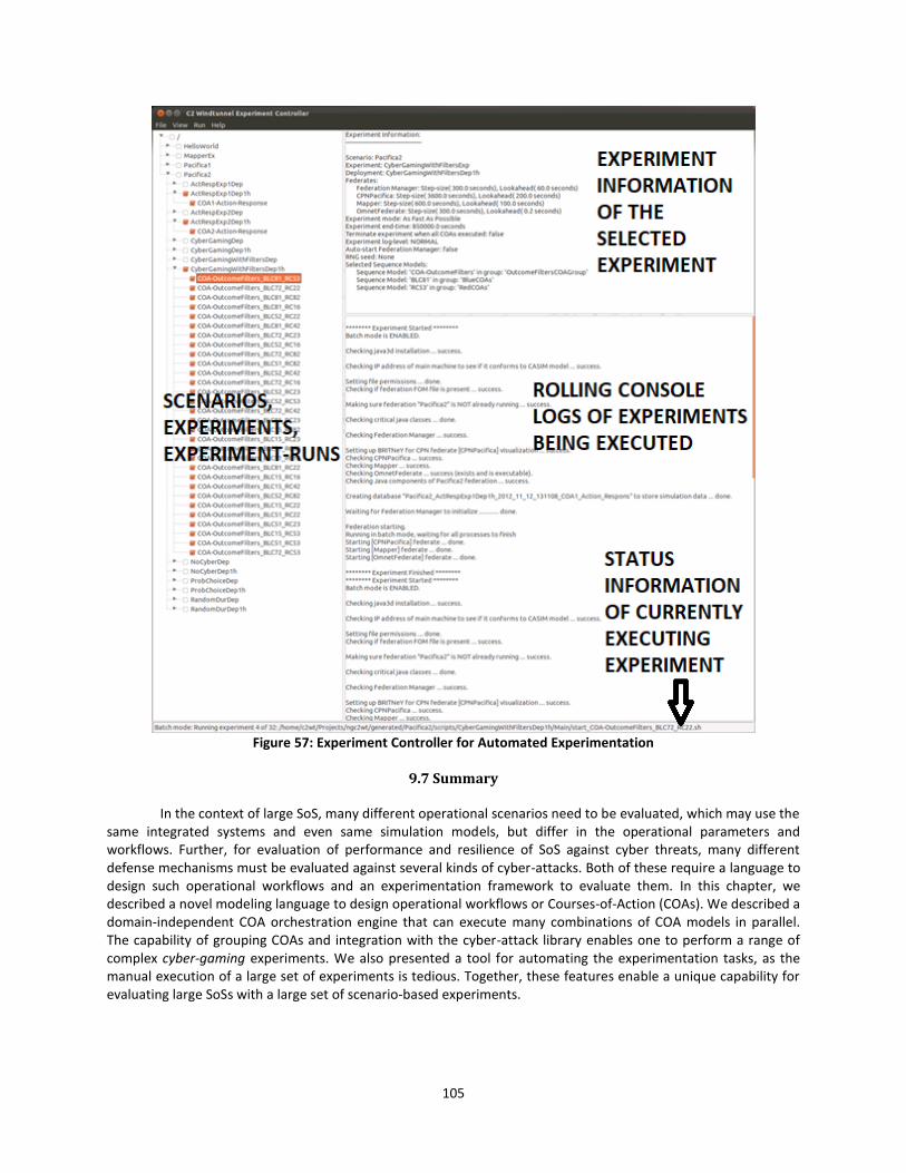
105

Figure 57: Experiment Controller for Automated Experimentation

9.7 Summary

In the context of large SoS, many different operational scenarios need to be evaluated, which may use the same integrated systems and even same simulation models, but differ in the operational parameters and workflows. Further, for evaluation of performance and resilience of SoS against cyber threats, many different defense mechanisms must be evaluated against several kinds of cyber-attacks. Both of these require a language to design such operational workflows and an experimentation framework to evaluate them. In this chapter, we described a novel modeling language to design operational workflows or Courses-of-Action (COAs). We described a domain-independent COA orchestration engine that can execute many combinations of COA models in parallel. The capability of grouping COAs and integration with the cyber-attack library enables one to perform a range of complex cyber-gaming experiments. We also presented a tool for automating the experimentation tasks, as the manual execution of a large set of experiments is tedious. Together, these features enable a unique capability for evaluating large SoSs with a large set of scenario-based experiments.

106

10. ONTOLOGY-BASED MODEL COMPOSITION

10.1 Introduction

Ontologies are well suited to capture knowledge base of a simulation tool’s input-output interfaces, particularly in the context of large SoSs. Large SoSs are complex to evaluate, but also present unique opportunity to integrate simulation tools using only those inputs and outputs that are relevant for the integrated simulations. The number of inputs and outputs that need to be considered for integration is usually much smaller than all the interfaces that a simulation tool may have. In this context, ontologies can effectively model the simulator’s input and output interfaces and the information flowing through them.

The reader is referred to Section 2.4.2 for a background on ontologies. In addition, we previously described the related work in using ontologies for simulation composition in Section 2.4.3. One of the fundamental issues in distributed simulations is that often it is not possible to use a common data model for some of the simulations. This can happen if either the source code of the simulator is not available, or it is highly tedious to modify it to perform translation of messages in the common data model to that used internally by the simulator, or it is not desirable to recompile the simulation source code for handling different scenario-specific data elements. Therefore, a mapper engine is needed that can translate messages between the two formats. Previously, in Chapter 5, we described the mapping methods developed in our research and how a mapper could be generated using the mapping specifications provided in the models. However, as the data model used in the scenarios grows and the number of messages that need to be translated increases, the number of mappings required also grows rapidly. In addition, the specification of mappings in a Java-like syntax becomes highly tedious when faced with specifying a large number of mappings in the model. Furthermore, as the models are developed in an iterative manner with gradual changes, it is often required to rework the previously specified mappings. Consequently, the solutions developed thus far can become hard to use and maintain.

The key idea described in this chapter is to leverage the power of ontological specification of simulation tool interfaces and use that specification to drive automated integration of these simulations. The framework language and tools need to be extended to allow specifying ontologies on simulations and their inputs and outputs. In addition, a new modeling language is needed to specify the rules of mapping inputs and outputs of one simulation tool to the other. The language should allow specifying detailed mapping rules as well as guard conditions. Together, this set of concepts can create reusable framework extensions for specifying ontology-based mapping rules. Finally, an automated mapping engine is needed that can use the specified mapping rules and generate mappings that enables the simulation tools to interoperate.

Ontological mapping specifications and automation in deriving specific mappings using ontological mapping rules can provide a significant benefit in rapid composition of simulation models, thus enabling even rapid experiment generation and evaluation even when the scenarios change significantly. In this chapter, we describe our research on using ontologies and ontological mapping rules for composing simulation models. The rest of the chapter is organized as follows. In Section 10.2, we present an Ontology Modeling Language (OML) for modeling domain-specific ontologies and Ontological Mapping Rules (OMRs). Next, in Section 10.3, we describe how to create the ontology and mapping rule models in GME. A detailed case study is presented in Section 10.4. Finally, in Section 10.5, we summarize the chapter.

107

10.2 Ontology Modeling Language

The basic elements of an ontology include the core concepts in the ontology, features associated with those concepts, and relations among those concepts. Figure 58 shows the metamodel of our Ontology Modeling Language (OML).

Figure 58: Ontology Modeling Language (OML)

As shown in Figure 58, the central element of an ontology is SPConcept. All ontological concepts must be

mapped to SPConcept in scenario models. The SPConcept can be hierarchically composed by allowing SPConcept models to contain other models of type SPConcept. SPConcept contains a SPIdentity model that identifies the model in the large collection of concepts in the scenario ontology. SPConcept can also contain a set of features of type SPFeature. SPFeature are mainly of these four types:

1. SPFixedValueFeature: These are the concept properties with a pre-defined data type and a value. 2. SPRangeValueFeature: This is used to specify a range of data values that the feature can take. The field

SPFeatureDataType denotes the data types for the values specified in the SPRangeExpression field. 3. SPEnumeratedValueFeature: This is used to specify a set of pre-defined enumerations, which are defined

using a SPFeatureDataType for the data type of the enumerated value, and a SPFeatureValue to capture the actual value of the enumerated item.

4. SPInstanceValueFeatures: This includes feature values that are themselves features.

108

In addition, SPConcept is also a member of an equivalence relation denoted by SPConceptEquivalence. The main idea of an equivalence relation is to specify the same physical concepts in the real world being denoted by different SPConcepts in different domain-specific ontologies.

Figure 59 shows the metamodel for OMRs. Different domain-specific ontologies are created for the different models. For example, when a remote operator function is simulated along with a simulation of the communication network, two different ontologies could be defined, viz. operations ontology and the communication network ontology. For the message sent between two nodes inside the operations ontology, a message is translated to go through the simulated network prior to delivering it to the destination element node.

The idea is to enable specification of mapping rules between a sender and receiver ontological concept in one ontological domain (called the source ontology) to the corresponding sender and receiver concept pair in another ontological domain (called the destination ontology). For example, if a message from the remote operator to a remotely controlled instrument is to be sent over a simulated network, then this message must be translated into the communication network ontology and must be sent from network node corresponding to the operator to the network node corresponding to the remotely controlled instrument.

Mappings are needed not just for the messages sent over the simulated network, but also for messages translated between any pair of ontological domains. For example, consider a simulation of physical dynamics of a system that sends signal updates to a receiving node. This message may need to be mapped to a corresponding message in an interconnected simulation of sensor fusion algorithms. Here, the message is not routed through a simulated network, but the two ontological domains, viz. physics simulation and sensor fusion, are interdependent and need to map messages sent in their respective domain to the other.

An Ontological Mapping Rule (OMR) always has an associated ‘sender’ concept from the source ontology. The initiation of a message sent in the source ontology by the sender concept triggers the mapping rule. Depending on the requirements (and restrictions) of the mappings, the mapping rule may include the associated ‘receiver’ concept from the source ontology as well as the corresponding ‘sender’ and ‘receiver’ concepts from the destination ontology.

As shown in Figure 59, the sender and receiver concepts refer to the associated HLA interaction, which is the message type in that ontological domain. In our implementation, there are always two such interactions in a mapping rule, one from both the source and destination ontologies.

When the general ontological concepts are used to create mapping rules, they apply to all of the ontological concepts that are derived from those concepts in that ontological domain. This is how the OMRs are supposed to work. However, in some applications, this can result in the rule being applied to some undesired combinations. We provide detailed examples in the case study in Section 10.5. However, for now, consider a sensor network domain with sensor nodes and senor fusion nodes. Assuming that these sensors are spread across an area and there are different fusion nodes in different areas. Here the message sent from sensors in one area should go to the fusion node only in that area. A general mapping rule specification will allow sending to all derivatives of the fusion node concept. For this reason, as shown in Figure 59, we extended the modeling language to allow specification of exclusions and restrictions in mapping rules. A sender-receiver exclusion in the rule allows the rule to be applied for all pairs of derivatives of the sender and receiver concepts, except for those explicitly specified. On the other hand, a sender-receiver restriction in the rule disables the rules application for all pairs of derivatives of the sender and receiver concepts, while permitting only those explicitly specified.

109

Figure 59: Meta-Model for Ontological Mapping Rules

110

10.3 Creating Ontologies and Mapping Rules

In this section, we describe how to create ontologies and OMRs using the modeling language in our framework.

“An important point to note is that when a domain-specific ontology is created, we do not need to model all of the concepts in that domain. This is significantly different from existing approaches (see Section 2.4.3) where focus is more on creating expansive ontologies that cover most of the concepts in the ontological domain.” In our framework, we require definitions of only those concepts that are pertinent to any of the OMRs

that are included in experiments. This significantly alleviates the burden of creating all-encompassing ontologies. Secondly, this makes our ontologies highly specific to the application domain of the SoS where these concepts are used directly. This makes it easier for domain experts to create such ontologies. Thirdly, the level of detail captured for the ontological concepts is also required to contain only that amount of information that is relevant for the current SoS application domain. Finally, it is still permissible to include as many concepts as desired with as much detail in them in our ontologies. The extra information is not used, but may have performance impact only at the time of code-generation, but negligible during run-time.

10.3.1 Ontology Modeling

Ontology for a new ontological domain is created by first creating a model of type ‘SPOntology’. Table 4 shows the icons and descriptions for elements of ontological models in our OML. Inside a SPOntology model, the designer starts by first creating a root/parent SPConcept model that is reflective of the overall ontological domain (e.g. SensorNetwork, CommunicationNetwork). Next, the top-level concepts are created as models of type ‘SPConcept’ and a containment relation is created from these top-level concepts to the root/parent concept. Table 4 shows the default icon for a SPConcept model, which is usually overridden by a more domain-specific icon. SPConcept contains a child model of type ‘SPIdentity’ and a set of features that can be any of the four types, viz. SPFixedValueFeature, SPRangeValueFeature, SPEnumeratedValueFeature, or SPInstanceValueFeature (these were described previously in Section 10.2).

After creating the top-level concepts, these concepts can be refined to create derivative concepts. This is done by creating them as ‘SubType’ of parent SPConcept models in GME. The parent and derivative concepts can be used to create ‘Instance’ models in GME in the OMRs.

Figure 60 shows an example SPConcept model for the concept of a network ‘Host’ in a communication network ontology. As shown, the concept is defined by first creating its SPIdentity model. A SPIdentity model can contain models of type SPId and SPName. In this example, it contains only a SPId called ‘NetworkElementId’ with data type ‘String’ and a default value ‘NEx’. The default value is overridden in derivative concepts, e.g. ‘WirelessHost’. Next, two features are defined of type ‘SPEnumeratedValuesFeature’ called ‘NetworkInterfaces’ and ‘TransportProtocols’. The figure shows the enumerated values inside those features.

We provide detailed examples of ontologies in the case study in Section 10.5.

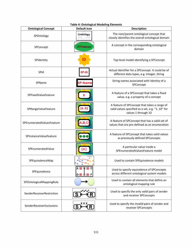
111

Table 4: Ontological Modeling Elements

Ontological Concept Default Icon Description

SPOntology

The root/parent ontological concept that closely identifies the overall ontological domain

SPConcept

A concept in the corresponding ontological domain

SPIdentity

Top-level model identifying a SPConcept

SPId

Actual identifier for a SPConcept. It could be of different data types, e.g. Integer, String

SPName

String names associated with identity of a SPConcept

SPFixedValueFeature

A feature of a SPConcept that takes a fixed value, e.g. a property of a concept

SPRangeValueFeature

A feature of SPConcept that takes a range of valid values specified as a set, e.g. “1..10” for

values 1 through 10

SPEnumeratedValuesFeature

A feature of SPConcept that has a valid set of values that are pre-defined as an enumeration

SPInstanceValueFeature

A feature of SPConcept that takes valid values as previously defined SPConcepts

SPEnumeratedValue

A particular value inside a SPEnumeratedValuesFeature model

SPEquivalenceMap

Used to contain SPEquivalence models

SPEquivalence

Used to specify equivalence of SPConcepts across different ontological system models

SPOntologicalMappingRule

Used to contain all elements that define an ontological mapping rule

SenderReceiverRestriction

Used to specify the only valid pairs of sender and receiver SPConcepts

SenderReceiverExclusions

Used to specify the invalid pairs of sender and receiver SPConcepts

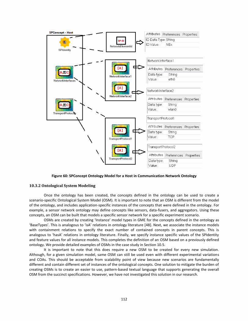
112

Figure 60: SPConcept Ontology Model for a Host in Communication Network Ontology

10.3.2 Ontological System Modeling

Once the ontology has been created, the concepts defined in the ontology can be used to create a scenario-specific Ontological System Model (OSM). It is important to note that an OSM is different from the model of the ontology, and includes application-specific instances of the concepts that were defined in the ontology. For example, a sensor network ontology may define concepts like sensors, data-fusers, and aggregators. Using these concepts, an OSM can be built that models a specific sensor network for a specific experiment scenario.

OSMs are created by creating ‘Instance’ model types in GME for the concepts defined in the ontology as ‘BaseTypes’. This is analogous to ‘isA’ relations in ontology literature [48]. Next, we associate the instance models with containment relations to specify the exact number of contained concepts in parent concepts. This is analogous to ‘hasA’ relations in ontology literature. Finally, we specify instance specific values of the SPIdentity and feature values for all instance models. This completes the definition of an OSM based on a previously defined ontology. We provide detailed examples of OSMs in the case study in Section 10.5.

It is important to note that this does require a new OSM to be created for every new simulation. Although, for a given simulation model, same OSM can still be used even with different experimental variations and COAs. This should be acceptable from scalability point of view because new scenarios are fundamentally different and contain different set of instances of the ontological concepts. One solution to mitigate the burden of creating OSMs is to create an easier to use, pattern-based textual language that supports generating the overall OSM from the succinct specifications. However, we have not investigated this solution in our research.

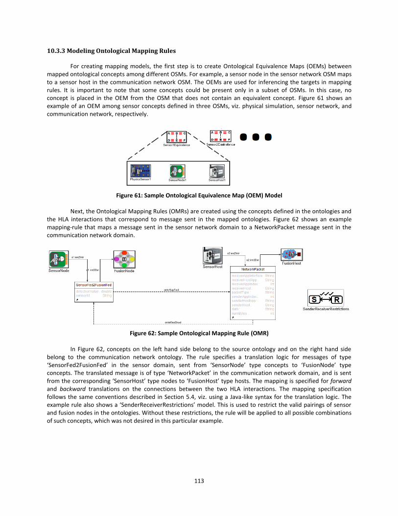
113

10.3.3 Modeling Ontological Mapping Rules

For creating mapping models, the first step is to create Ontological Equivalence Maps (OEMs) between mapped ontological concepts among different OSMs. For example, a sensor node in the sensor network OSM maps to a sensor host in the communication network OSM. The OEMs are used for inferencing the targets in mapping rules. It is important to note that some concepts could be present only in a subset of OSMs. In this case, no concept is placed in the OEM from the OSM that does not contain an equivalent concept. Figure 61 shows an example of an OEM among sensor concepts defined in three OSMs, viz. physical simulation, sensor network, and communication network, respectively.

Figure 61: Sample Ontological Equivalence Map (OEM) Model

Next, the Ontological Mapping Rules (OMRs) are created using the concepts defined in the ontologies and

the HLA interactions that correspond to message sent in the mapped ontologies. Figure 62 shows an example mapping-rule that maps a message sent in the sensor network domain to a NetworkPacket message sent in the communication network domain.

Figure 62: Sample Ontological Mapping Rule (OMR)

In Figure 62, concepts on the left hand side belong to the source ontology and on the right hand side

belong to the communication network ontology. The rule specifies a translation logic for messages of type ‘SensorFed2FusionFed’ in the sensor domain, sent from ‘SensorNode’ type concepts to ‘FusionNode’ type concepts. The translated message is of type ‘NetworkPacket’ in the communication network domain, and is sent from the corresponding ‘SensorHost’ type nodes to ‘FusionHost’ type hosts. The mapping is specified for forward and backward translations on the connections between the two HLA interactions. The mapping specification follows the same conventions described in Section 5.4, viz. using a Java-like syntax for the translation logic. The example rule also shows a ‘SenderReceiverRestrictions’ model. This is used to restrict the valid pairings of sensor and fusion nodes in the ontologies. Without these restrictions, the rule will be applied to all possible combinations of such concepts, which was not desired in this particular example.

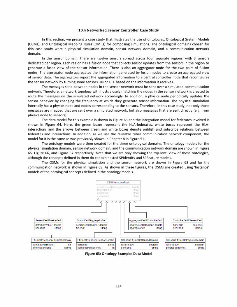
114

10.4 Networked Sensor Controller Case Study

In this section, we present a case study that illustrates the use of ontologies, Ontological System Models (OSMs), and Ontological Mapping Rules (OMRs) for composing simulations. The ontological domains chosen for this case study were a physical simulation domain, sensor network domain, and a communication network domain.

In the sensor domain, there are twelve sensors spread across four separate regions, with 3 sensors dedicated per region. Each region has a fusion node that collects sensor updates from the sensors in the region to generate a fused view of the sensor information. There is also an aggregator node for the two pairs of fusion nodes. The aggregator node aggregates the information generated by fusion nodes to create an aggregated view of sensor data. The aggregators report the aggregated information to a central controller node that reconfigures the sensor network by turning some sensors ON or OFF based on the information it receives.

The messages send between nodes in the sensor network must be sent over a simulated communication network. Therefore, a network topology with hosts closely matching the nodes in the sensor network is created to route the messages on the simulated network accordingly. In addition, a physics node periodically updates the sensor behavior by changing the frequency at which they generate sensor information. The physical simulation internally has a physics node and nodes corresponding to the sensors. Therefore, in this case study, not only those messages are mapped that are sent over a simulated network, but also messages that are sent directly (e.g. from physics node to sensors).

The data model for this example is shown in Figure 63 and the integration model for federates involved is shown in Figure 64. Here, the green boxes represent the HLA-federates, white boxes represent the HLA-interactions and the arrows between green and white boxes denote publish and subscribe relations between federates and interactions. In addition, as we use the reusable cyber communication network component, the model for it is the same as was previously shown in Chapter 8 in Figure 51.

The ontology models were then created for the three ontological domains. The ontology models for the physical simulation domain, sensor network domain, and the communication network domain are shown in Figure 65, Figure 66, and Figure 67 respectively. Note that we are only showing the top-level view of these ontologies, although the concepts defined in them do contain nested SPIdentity and SPFeature models.

The OSMs for the physical simulation and the sensor network are shown in Figure 68 and for the communication network is shown in Figure 69. As shown in these figures, the OSMs are created using ‘Instance’ models of the ontological concepts defined in the ontology models.

Figure 63: Ontology Example: Data Model

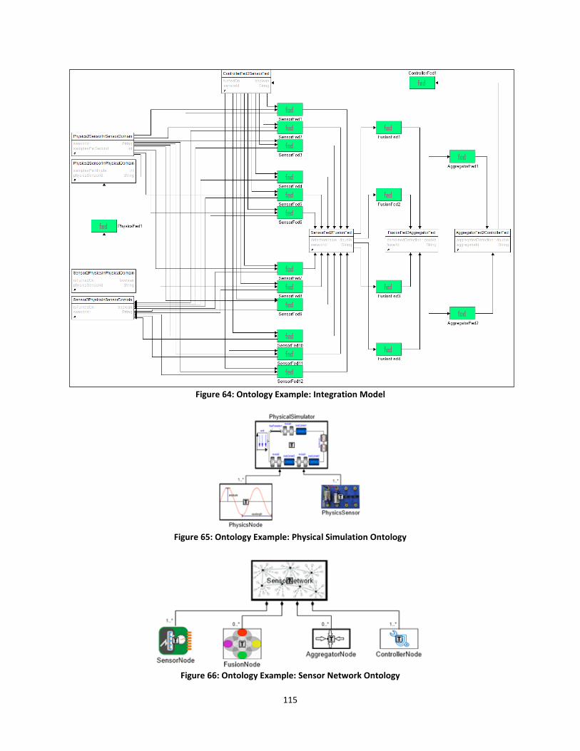
115

Figure 64: Ontology Example: Integration Model

Figure 65: Ontology Example: Physical Simulation Ontology

Figure 66: Ontology Example: Sensor Network Ontology

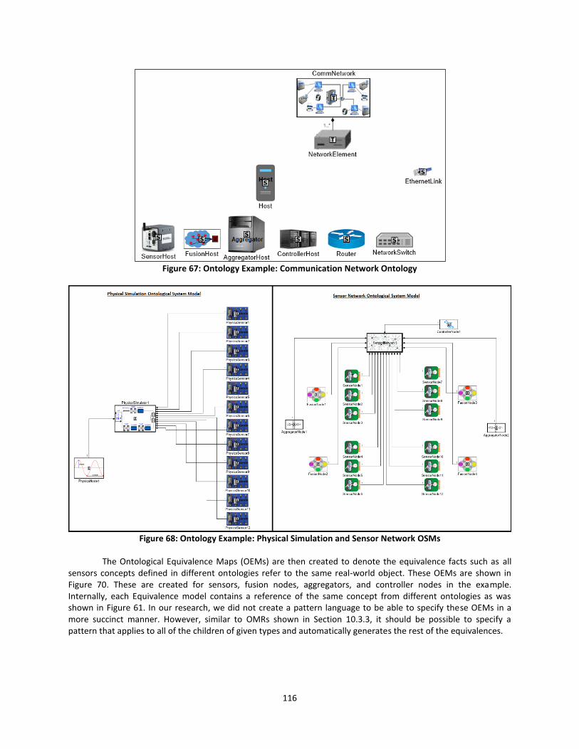
116

Figure 67: Ontology Example: Communication Network Ontology

Figure 68: Ontology Example: Physical Simulation and Sensor Network OSMs

The Ontological Equivalence Maps (OEMs) are then created to denote the equivalence facts such as all

sensors concepts defined in different ontologies refer to the same real-world object. These OEMs are shown in Figure 70. These are created for sensors, fusion nodes, aggregators, and controller nodes in the example. Internally, each Equivalence model contains a reference of the same concept from different ontologies as was shown in Figure 61. In our research, we did not create a pattern language to be able to specify these OEMs in a more succinct manner. However, similar to OMRs shown in Section 10.3.3, it should be possible to specify a pattern that applies to all of the children of given types and automatically generates the rest of the equivalences.

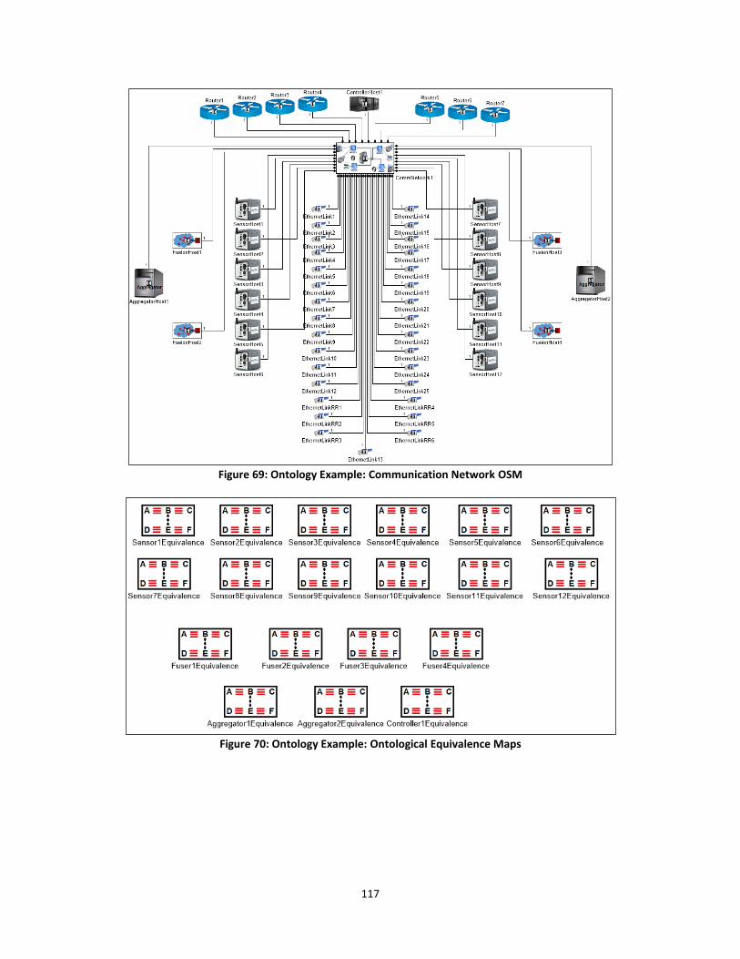
117

Figure 69: Ontology Example: Communication Network OSM

Figure 70: Ontology Example: Ontological Equivalence Maps

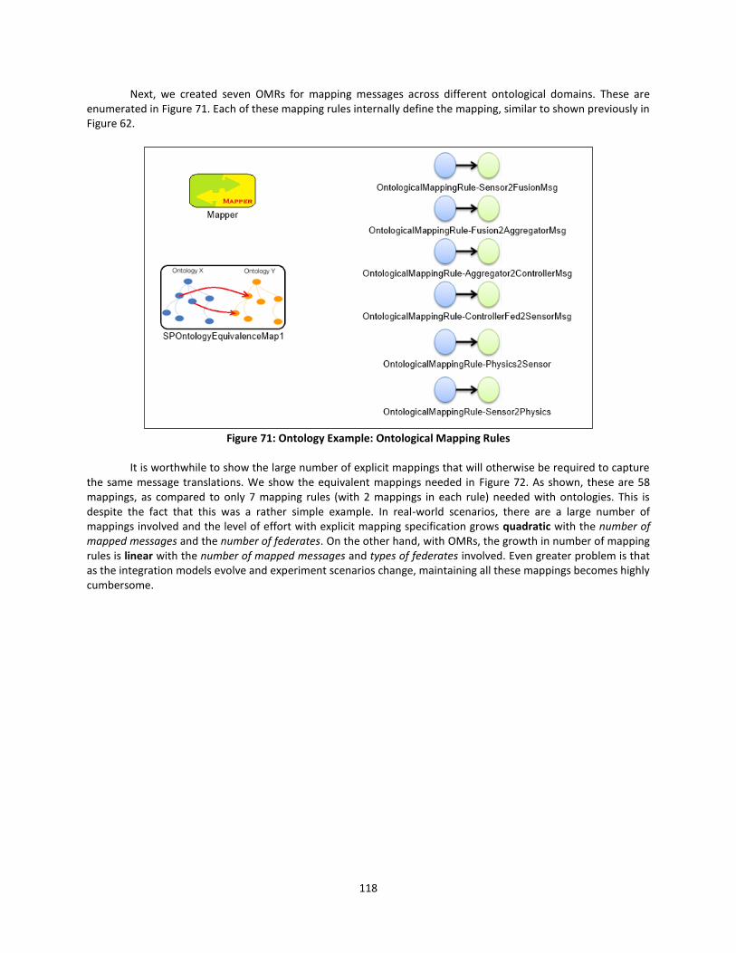
118

Next, we created seven OMRs for mapping messages across different ontological domains. These are enumerated in Figure 71. Each of these mapping rules internally define the mapping, similar to shown previously in Figure 62.

Figure 71: Ontology Example: Ontological Mapping Rules

It is worthwhile to show the large number of explicit mappings that will otherwise be required to capture

the same message translations. We show the equivalent mappings needed in Figure 72. As shown, these are 58 mappings, as compared to only 7 mapping rules (with 2 mappings in each rule) needed with ontologies. This is despite the fact that this was a rather simple example. In real-world scenarios, there are a large number of mappings involved and the level of effort with explicit mapping specification grows quadratic with the number of mapped messages and the number of federates. On the other hand, with OMRs, the growth in number of mapping rules is linear with the number of mapped messages and types of federates involved. Even greater problem is that as the integration models evolve and experiment scenarios change, maintaining all these mappings becomes highly cumbersome.

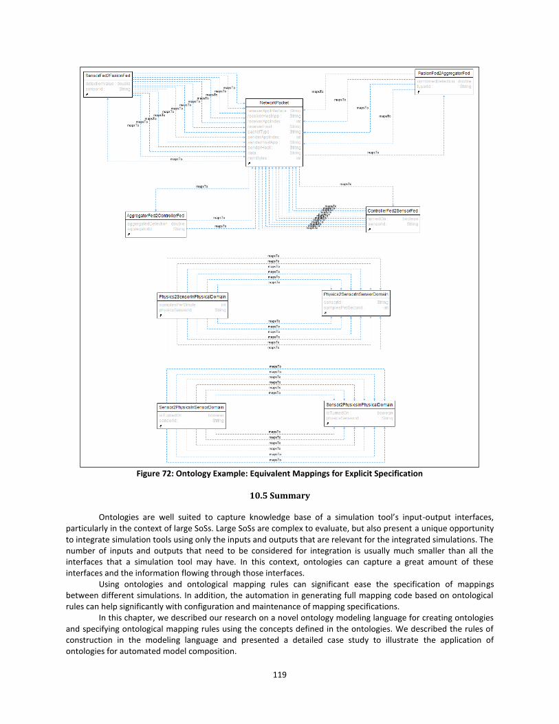
119

Figure 72: Ontology Example: Equivalent Mappings for Explicit Specification

10.5 Summary

Ontologies are well suited to capture knowledge base of a simulation tool’s input-output interfaces, particularly in the context of large SoSs. Large SoSs are complex to evaluate, but also present a unique opportunity to integrate simulation tools using only the inputs and outputs that are relevant for the integrated simulations. The number of inputs and outputs that need to be considered for integration is usually much smaller than all the interfaces that a simulation tool may have. In this context, ontologies can capture a great amount of these interfaces and the information flowing through those interfaces.

Using ontologies and ontological mapping rules can significant ease the specification of mappings between different simulations. In addition, the automation in generating full mapping code based on ontological rules can help significantly with configuration and maintenance of mapping specifications.

In this chapter, we described our research on a novel ontology modeling language for creating ontologies and specifying ontological mapping rules using the concepts defined in the ontologies. We described the rules of construction in the modeling language and presented a detailed case study to illustrate the application of ontologies for automated model composition.

120

11. RESULTS, CONCLUSIONS, FUTURE WORK, AND BROADER IMPACT

11.1 Results

In this section, we evaluate the methods, tools, and approaches developed in this research against the challenge problems identified in Chapter 3. The evaluation should validate the research hypothesis or reflect the reasons for its invalidity.

11.1.1 Challenge Problems Addressed

First, we go the challenge problems identified for this research work and describe how they were addressed.

11.1.1.1 Challenge Problem 1

Problem statement: How can we create an integrative framework that supports model-based distributed simulation and its fundamental requirements for modeling, configuring, and experimentation? The framework must provide a modeling language to create system integration models, generators to synthesize artifacts programmatically from the integration models to implement and configure the distributed simulation, a controller to control the distributed simulation, and tools and techniques for automated deployment of simulations on computers as well as executing them. Solutions developed: In this research work, we developed a model-based simulation integration and experimentation framework that enables researchers to integrate and evaluate large SoS simulations, and assess, evaluate, and validate their algorithms in realistic scenarios. In this framework, it is possible to integrate domain-specific models rapidly from diverse simulation engines and to generate all of the needed configuration and integration code dynamically. The environment also provides automated facilities to manage the deployment and execution of the simulation itself. Together these tools greatly reduce the time required to design, modify, and test large SoS simulation scenarios. These solutions are described in Chapter 4 of this dissertation.

11.1.1.2 Challenge Problem 2 Problem statement: How can we support legacy simulation tools that have fixed data models for which they work? Automatic mapping techniques are needed for translating messages between the fixed data model format used by the legacy simulation tools and the common data model used by the rest of the distributed simulation. Solutions developed: In this research work, we developed the tools and methods for supporting legacy components through mapping methods. Essentially, these methods allow translation of messages between the commonly agreed data model and the one used by the legacy component. We developed a custom modeling language to define mappings and code generator to generate a mapper federate that executes synchronously with the rest of the simulation and translates messages as they are sent by other federates according to the specification provided in mapping models. These solutions are described in Chapter 5 of this dissertation.

11.1.1.3 Challenge Problem 3 Problem statement: How can we create a reusable component for communication network simulation that can be easily configured and reused for many different network topologies that may be needed in different distributed simulation scenarios? Solutions developed: In this research work, we developed a reusable cyber communication network simulation component called OmnetFederate. OmnetFederate has an extensible architecture that allows it to be used in many different experiment scenarios, and makes it easier to extend for additional networking behaviors and protocols. These solutions are described in Chapter 6 of this dissertation.

121

11.1.1.4 Challenge Problem 4 Problem statement: How can we support dynamic models partitioned into separate FMUs across sampling rate boundaries? The framework should support FMUs as one of the simulation components and it should support executing different FMUs at different step-sizes. Solutions developed: In this research work, we developed a solution to enable such partitioning of the model using the FMI standard for packaging the split models and executing them together as HLA federates. We also described a fully automated framework for modeling and execution of the split models. In addition, we provided guidelines for systematically partitioning the models and tuning their step-sizes to improve the simulation performance. These solutions are described in Chapter 7 of this dissertation.

11.1.1.5 Challenge Problem 5 Problem statement: How can we create a reusable cyber-attack library for evaluating how cyber-attacks can affect system behavior and how resilient its security mechanisms are to mitigate these effects? The library should allow selecting, configuring, and applying a variety of reusable cyber-attacks at various network elements. Solutions developed: In this research work, we developed a reusable and modular cyber-attack library that allows experimenters to 'plug-in' many different cyber-attacks at different time-points and network nodes in the SoS simulations. In this library, we developed models for a number of cyber-attacks that are useful for evaluating SoS's performance and reliability such as Distributed Denial of Service (DDoS) attacks, network delays, data corruption, network manipulation, and integrity attacks. The cyber-attack library is domain-independent and it is up to the experimenters to pick the set of cyber-attacks to deploy as test conditions in their experiments. These solutions are described in Chapter 8 of this dissertation.

11.1.1.6 Challenge Problem 6 Problem statement: How can we support scenario-driven experimentation to study the emergent behavior of the distributed simulation under several what-if scenarios? The required capabilities include modeling, configuring, executing, and monitoring of multiple, parallel courses-of-action. Solutions developed: In this research work, we developed a novel modeling language to design operational workflows, called Courses-of-Action (COAs). We described a domain-independent COA orchestration engine that can execute many combinations of COA models in parallel. The capability of grouping COAs and integration with the cyber-attack library enables one to perform a range of complex cyber-gaming experiments. We also presented a tool for automating the experimentation tasks, as the manual execution of a large set of experiments is tedious. Together, these features enable a unique capability for evaluating large SoSs with a large set of scenario-based experiments. These solutions are described in Chapter 9 of this dissertation.

11.1.1.7 Challenge Problem 7 Problem statement: How can we use ontologies for automatically compose models in different domains? For example, a road traffic simulation understands traffic flows and associated variables, but a communication network only works with network packets. In order to study the integrated system behavior, these two models must be composed together. Ontology-based tools and techniques are needed to automate this composition. Solutions developed: In this research work, we developed a novel ontology modeling language for creating ontologies and specifying ontological system models and ontological mapping rules using the concepts defined in the ontologies. We described the rules of construction in the modeling language and presented a detailed case study to illustrate the application of ontologies for automated model composition. These solutions are described in Chapter 10 of this dissertation.

122

11.1.2 Evaluation of Research Hypothesis with Research Results

Research Hypothesis:

“Model-based rapid synthesis of distributed HLA-based simulations is implementable as a reusable and integrative distributed simulation framework and can support mapping methods for legacy component interfaces, reusable component for communication network simulation, multi-rate model partitioning using FMU-CS, modeling and integration of cyber-attacks, scenario-driven experimentation using courses of action evaluation, and ontology-based model composition. Such an integrative framework should help system integrators with rapidly synthesizing distributed simulations while handling multiple of above problems; as well as provide intelligent composition of models.”

Evaluation of Research Hypothesis: Distributed simulation based on HLA is a highly tedious task because not only different tools need to be

made conformant with HLA, but also evolving them with changing requirements. Our hypothesis claimed that a model-based distributed HLA-based simulations could be synthesized using a reusable and integrative framework. This is validated with the fact that our framework developed tools for HLA-adapter code generation, simulation deployment, simulation control, and automated experimentation, and that it can be directly used for synthesizing HLA-based distributed simulations and experimentation with those simulations. We described these results in Chapter 4.

In our research hypothesis, we also claimed that this framework could support mapping methods for legacy component interfaces. Our research demonstrated that, with mapping methods, legacy components could indeed be interfaced with and integrated into the distributed simulation. We described these results in Chapter 5.

Another research hypothesis claim was that we could develop a reusable component in this integration framework to support communication network simulation. As described in Chapter 6, the reusable component we developed can be used in different application domains without modifications.

We also hypothesized that multi-rate partitioning of complex models could be supported using FMI Co-Simulation Units. In Chapter 7, we showed how a complex Modelica model can be partitioned across sampling rate boundaries and different partitions could be executed using different step-sizes. We also provided a detailed case study to validate this claim further.

The next hypothesis we claimed was that in this framework, one could support modeling and integration of cyber-attacks. In our research, as described in Chapter 8, we not only showed that this is possible, but we went further by developing a reusable cyber-attack library, that is integrated into the framework and is accessed using appropriate modeling constructs, thus validating the hypothesis claim.

Our research hypothesis also claimed that the framework could support scenario-driven experimentation using courses-of-action evaluation. We showed in Chapter 9, a novel modeling language for creating COA models and described the techniques we developed in orchestrating the COAs automatically. The COA modeling language and tools for orchestrating COA models validate this hypothesis claim.

Finally, in our research hypothesis, we claimed that ontologies could be used for composing simulation models. In Chapter 10, we described a novel modeling language to create ontologies, ontological system models, and ontological mapping rules. We also demonstrated how a mapper based on the ontology models could translate messages among distinct ontological domains, thus validating the hypothesis claim.

123

11.2 Conclusions

Large system-of-systems are highly complex and composed of several interdependent systems. This makes their evaluation rather challenging. Physical validation and formal analysis are not manageable for their evaluations, as these are either uneconomical, unsafe, or highly complex. Integrated simulations are preferred means for evaluating these systems. However, this requires both integrating the heterogeneous models in different system domains (physical, computational, or human), and integrating the heterogeneous simulators in different domains. This is challenging because heterogeneous models may have highly different semantics and the heterogeneous simulators may use different methods for handling simulation time and events. Addressing these challenges of heterogeneity requires integrating simulations in a logically and temporally consistent manner.

The IEEE HLA standard provides a well-defined API for creating and experimenting with distributed simulations. However, adapting simulations to comply with the HLA standard is complex and manual processes are rather tedious and unmaintainable due to evolving requirements and models. In this research, we developed a model-based integration framework to rapidly synthesize HLA-based distributed simulations. The framework also developed tools and methods to meet several real-world simulation-based experimentation requirements. Using this framework, complex integrated simulations could be developed and experimented with within minutes, which, when developed though manual processes could take several days to create.

In our research, we also developed mapping methods and techniques to support legacy component interfaces. This is a highly useful result because many of the existing simulators do not permit source code modifications and use a pre-defined input and output model. One interesting results was that the mapping methods developed was directly used in creating a reusable network simulation component that needed to fix its input and output model to be used in a generic manner. Another result we derived from our work on partitioning dynamic models across rate boundaries was that such partitioning is not only doable, but is useful in gaining simulation performance, particularly when the dynamical models are large, complex, and exhibit different rate dynamics in different parts of the model. The reusable cyber-attack library developed in this research is highly useful tool for evaluating complex SoS against cyber threats. In addition, the techniques to support evaluation of alternative courses-of-actions enabled cyber-gaming evaluations when COAs are coupled with the reusable cyber-attack library. Further, we developed a novel ontology modeling language to create ontologies and ontological mapping rules, which facilitate the burden of explicitly specifying a large number of mappings between composed models. The systematic approach to mapping creation makes it amenable to automatic specification using template based and artificial intelligence based techniques.

In this way, this research developed many generalizable integration techniques for general-purpose and standards-based large-scale simulation integration. The developed framework enables researchers to integrate and evaluate large SoS simulations, and assess, evaluate, and validate their algorithms in realistic scenarios.

11.3 Future Work

Large-scale integration of heterogeneous simulations is a highly complex topic. In this research, we have solved several of its core challenges. Further research can build upon the results of this research work. We identify several such opportunities for future work as follows:

1. The communication network is a central component that cuts across all interoperating systems. There is a potential for large overhead on simulation performance if a large number of networked messages are used between simulations or a large number of low-level network packets must be simulated. This is because the network simulator must simulate all network packet transmission faithfully for determining the network behavior. An open research problem is to be able to vary the fidelity of network simulation during run-time so that, when low-level packet simulation are not significant for the overall evaluation of the SoS, a lower fidelity model could significantly improve performance. However, first these two challenges must be solved: (i) techniques for dynamically switching between different fidelity levels must be devised, and (ii) consistency of internal network variables must be ensured across these transitions.

2. In Chapter 5, we developed mapping techniques for translating messages between simulators. We also described modeling of many-to-one type of mappings and that in real-world simulations, other mapping types are also needed such as one-to-many and many-to-many. However, these must be addressed in a way that preserves domain-specific semantics of translations. For example, when multiple sensor

124

messages are to be collected and mapped as a single block update, this update may have an associated frequency requirement with it. Secondly, it might be allowable to discard some input samples. Such issues can be addressed on a case-by-case basis; however, a precise analytical framework can be developed that addresses the need of specifying such requirements and handling them systematically.

3. Step-sizes of individual simulations have a significant impact on performance of the integrated simulation. In Chapter 7, we described a method to partition complex dynamical models into parts across different sampling rate boundaries using FMI for Co-Simulations (FMU-CS). This provides a performance benefit by allowing larger step-size for partitions that exhibit slower dynamics. However, simulations are known to exhibit varying rates of dynamics at different points in simulation. To take advantage of this, a technique can be devised to allow variation of step-sizes dynamically depending on current rate of dynamics exhibited by different simulation components.

4. Another interesting method could be to allow multiple ways of partitioning a complex dynamical model. In Chapter 7, we described a method to partition across sampling rate boundaries. It is possible, however, that this partitioning scheme is sub-optimal for some models. A general framework could be developed that allows partitioning across other dimensions such as physical domains (e.g. electrical, thermal), component architectures, and hierarchical granularity levels. Different partitioning schemes could be experimentally evaluated for domain-specific models for optimal performance.

5. Computation resource availability also plays a key role in simulation performance. A novel research direction is to develop techniques to monitor the run-time performance of participating simulators and change their allocations of computational resources dynamically depending on how much computational overhead they are currently experiencing at that time-point in the simulation.

6. The HLA standard allows for saving and restoring a partially completed distributed simulation. Many Run-Time Infrastructure implementations (such as Portico) also provide APIs for enabling this functionality. However, it is a challenging task for individual simulators to save their partial simulation states and then restore later from that point onwards. Secondly, after restoring the distributed simulation, all restored individual simulators must have their internal states consistent with each other. These needs addressing challenges of both saving and restoring individual simulators, as well as managing the overall integrated simulation states before and after the restore.

7. The emerging cloud computation platforms and web-based modeling tools make it possible to create a highly user-friendly, browser-based modeling and experimentation environment. However, in distributed simulations, the simulation models and software is created by the users of the simulations, which in a cloud environment require methods to version, manage, and compile them in a consistent manner. Having such capabilities can enable distributed simulations as online service platforms – a significant advantage for researchers that use integrated simulations for research in different application domains.

8. In Chapter 8, we described our research on creating a reusable cyber-attack library, containing several attack models that can be directly used for evaluating SoS against cyber threats. For cyber-attacks that do not directly map to the attacks in this library, it could be highly useful to develop a technique to take a trace file as an input to the network simulator for replicating the needed cyber-attack behavior. However, challenge arises in applying the trace file to exact network hosts, routes, and routing protocols.

9. In Chapter 10, we described our research on using ontologies and ontological mapping rules for automatic much of the mapping specifications among mapped messages across simulators. One interesting challenge problem is to develop Artificial Intelligence (AI) techniques to allow a natural language specification of ontological mapping rules. Alternatively, or in addition, higher-level templates could be devised to make rule specification much simpler. This allows user to specify the translation logic using, as opposed to programming constructs, a natural language specification.

10. Large SoS are highly complex and have many interdependencies among each other. Small variations of models and parameters can cause large changes in simulation results. Therefore, usually a large number of simulations are needed to arrive at meaningful results with a good degree of confidence. A system based on Artificial Intelligence (AI) could generate scenarios and parameter variations of these experiments, generate large data sets of experimental results, observe the simulation results against the scenario and parameter variations, and generate correlations between desired outcomes and alternative simulation trajectories. These could provide much greater insights for real-world mission situations that require simulation-based analysis for generating alternative mission plans.

125

11.4 Broader Impact

The framework developed in this research has already been applied for studies in several different application domains and transitioned to real-world simulation-based analysis platforms. This is a significant positive result. In addition, this research can also be extended toward addressing many research challenges (see Section 11.3 on future work). Furthermore, these research results can be effectively applied in many other application domains. We briefly describe below some of the areas where this research has been applied.

11.4.1 Simulation-based studies

The framework developed in this research has been successfully applied for several simulation-based studies. We describe four such studies below.

In Section 4.7, we presented a case study covering the operations of a large SoS involving tactical and operational decision making in the presence of an active adversary in a contested cyber environment.

Secondly, the framework was also used to demonstrate its application for supporting experimentation on resilient command and control to support mission assurance in a cyber-environment. The study focused on experimentation to understand a human-centric approach (humans responding to cyber-attacks based on detection and identification including countermeasures) to provide resilience in the presence of cyber-attacks.

Another application of the framework was for demonstrating its capability to support the evaluation of operational sequences that are prepared by and derived from Courses-of-Action by human experts. The case study was developed using a variety of scenarios unfolding in the world of Pacifica – an island of three nations – from the open-source Pacifica Crisis Scenario [128].

Another example of the application of this framework was for the design and analysis of complex Cyber-Physical Systems. Our institute previously developed the OpenMETA toolchain [129] for designing CPSs. It used simulations for analyzing different physics models of the CPSs such as thermal, electrical, and mechanical. As described earlier in Section 7.2.5, the large Dymola model was partitioned into two parts and were executed in an integrated manner using our framework’s support for HLA-based FMU Co-Simulations.

11.4.2 Research communities for web-based collaborative modeling and simulation

As the power-grid is evolving to include more green power generation technologies and more power consumers are becoming producers at the same time, it has become challenging to meet the continually changing power demand and supply. Transactive energy systems attempts to use variable power pricing based on demand and supply in order to manage the power-grid operations in a stable manner. This is a typical large SoS use-case. One interesting aspect in this use-case is that there are a large number of stakeholders needing to evaluate their own business models. This needs a large-scale distributed simulation of many such models, as they are interdependent. Therefore, these distributed simulations must be scalable. We leveraged our framework’s distributed simulation capabilities to create cloud-deployed and web- and model-based integration platform for transactive energy simulations [130] [131].

11.4.3 Transition to external lab as open-source tools

The US National Institute of Standards and Technology (NIST), in partnership our institute, developed a collaborative experiment development environment for integrating a variety of simulation tools with support for hardware-in-the-loop simulation and remote simulation components. This environment is called a Universal CPS Environment for Federation (UCEF) This has been made available in the public domain as an open-source project on GitHub [132]. A high-level workshop was conducted by NIST on July 27, 2017 to disseminate the information on UCEF into the larger co-simulation community in the power-grid application domain. UCEF uses the capabilities developed in our research for integrating the different simulation tools. This work is currently ongoing.

126

11.4.4 Web-based platform for CPS security and resilience researchers

The SecURE and REslient Cyber-Physical Systems (SURE) platform [133] is a web-based platform for evaluation of cybersecurity and performance impact and assessment of resilient monitoring and control algorithms. The platform uses smart transportation systems as the CPS application domain. For these evaluations, SURE uses realistic models of cyber and physical components and their interactions, realistic cyber-attack models, and operational test scenarios. Many case studies have been developed and demonstrated at different venues using the SURE platform, such as at [134]. Our framework is at the core of the SURE platform to support the distributed simulations executed in the cloud.

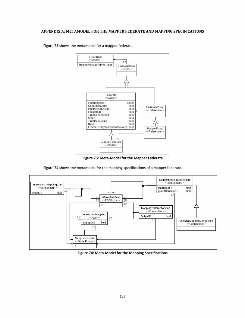
127

APPENDIX A: METAMODEL FOR THE MAPPER FEDERATE AND MAPPING SPECIFICATIONS

Figure 73 shows the metamodel for a mapper federate.

Figure 73: Meta-Model for the Mapper Federate

Figure 74 shows the metamodel for the mapping specifications of a mapper federate.

Figure 74: Meta-Model for the Mapping Specifications

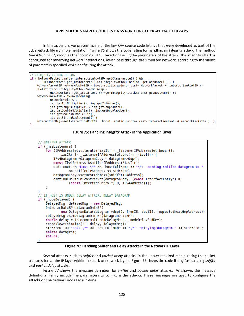
128

APPENDIX B: SAMPLE CODE LISTINGS FOR THE CYBER-ATTACK LIBRARY

In this appendix, we present some of the key C++ source code listings that were developed as part of the

cyber-attack library implementation. Figure 75 shows the code listing for handling an integrity attack. The method tweakIncoming() modifies the incoming HLA interactions using the parameters of the attack. The integrity attack is configured for modifying network interactions, which pass through the simulated network, according to the values of parameters specified while configuring the attack.

Figure 75: Handling Integrity Attack in the Application Layer

Figure 76: Handling Sniffer and Delay Attacks in the Network IP Layer

Several attacks, such as sniffer and packet delay attacks, in the library required manipulating the packet

transmission at the IP layer within the stack of network layers. Figure 76 shows the code listing for handling sniffer and packet delay attacks.

Figure 77 shows the message definition for sniffer and packet delay attacks. As shown, the message definitions mainly include the parameters to configure the attacks. These messages are used to configure the attacks on the network nodes at run-time.

129

Figure 77: Message Definitions for Sniffer and Packet Delay Attacks

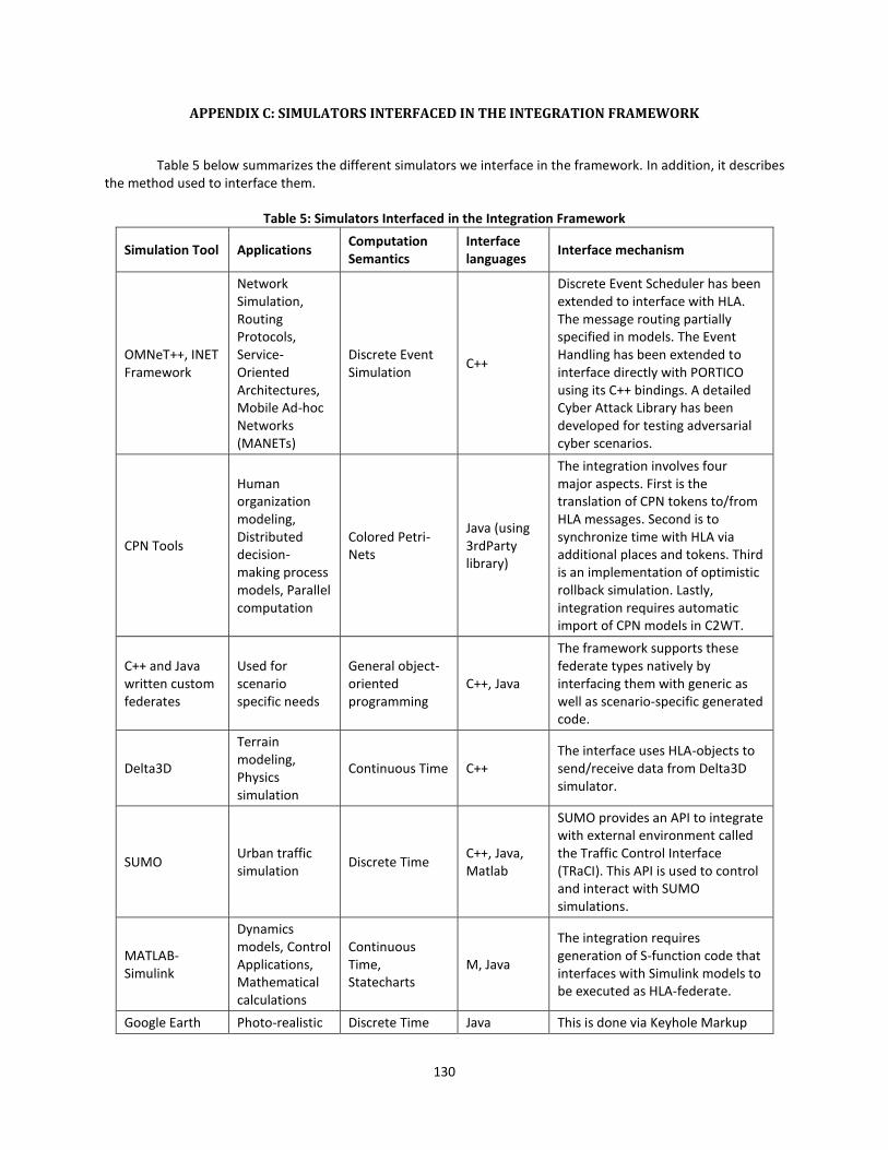
130

APPENDIX C: SIMULATORS INTERFACED IN THE INTEGRATION FRAMEWORK

Table 5 below summarizes the different simulators we interface in the framework. In addition, it describes

the method used to interface them.

Table 5: Simulators Interfaced in the Integration Framework

Simulation Tool Applications Computation Semantics

Interface languages

Interface mechanism

OMNeT++, INET Framework

Network Simulation, Routing Protocols, Service-Oriented Architectures, Mobile Ad-hoc Networks (MANETs)

Discrete Event Simulation

C++

Discrete Event Scheduler has been extended to interface with HLA. The message routing partially specified in models. The Event Handling has been extended to interface directly with PORTICO using its C++ bindings. A detailed Cyber Attack Library has been developed for testing adversarial cyber scenarios.

CPN Tools

Human organization modeling, Distributed decision-making process models, Parallel computation

Colored Petri-Nets

Java (using 3rdParty library)

The integration involves four major aspects. First is the translation of CPN tokens to/from HLA messages. Second is to synchronize time with HLA via additional places and tokens. Third is an implementation of optimistic rollback simulation. Lastly, integration requires automatic import of CPN models in C2WT.

C++ and Java written custom federates

Used for scenario specific needs

General object-oriented programming

C++, Java

The framework supports these federate types natively by interfacing them with generic as well as scenario-specific generated code.

Delta3D

Terrain modeling, Physics simulation

Continuous Time C++ The interface uses HLA-objects to send/receive data from Delta3D simulator.

SUMO Urban traffic simulation

Discrete Time C++, Java, Matlab

SUMO provides an API to integrate with external environment called the Traffic Control Interface (TRaCI). This API is used to control and interact with SUMO simulations.

MATLAB-Simulink

Dynamics models, Control Applications, Mathematical calculations

Continuous Time, Statecharts

M, Java

The integration requires generation of S-function code that interfaces with Simulink models to be executed as HLA-federate.

Google Earth Photo-realistic Discrete Time Java This is done via Keyhole Markup

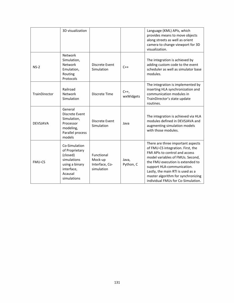
131

3D visualization Language (KML) APIs, which provides means to move objects along streets as well as orient camera to change viewport for 3D visualization.

NS-2

Network Simulation, Network Emulation, Routing Protocols

Discrete Event Simulation

C++

The integration is achieved by adding custom code to the event scheduler as well as simulator base modules.

TrainDirector Railroad Network Simulation

Discrete Time C++, wxWidgets

The integration is implemented by inserting HLA synchronization and communication modules in TrainDirector’s state update routines.

DEVSJAVA

General Discrete Event Simulation, Processor modeling, Parallel process models

Discrete Event Simulation

Java

The integration is achieved via HLA modules defined in DEVSJAVA and augmenting simulation models with those modules.

FMU-CS

Co-Simulation of Proprietary (closed) simulations using a binary interface, Acausal simulations

Functional Mock-up Interface, Co-simulation

Java, Python, C

There are three important aspects of FMU-CS integration. First, the FMI APIs to control and access model variables of FMUs. Second, the FMU execution is extended to support HLA-communication. Lastly, the main RTI is used as a master algorithm for synchronizing individual FMUs for Co-Simulation.

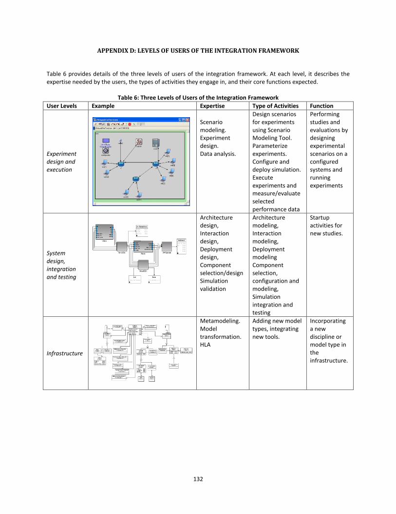
132

APPENDIX D: LEVELS OF USERS OF THE INTEGRATION FRAMEWORK

Table 6 provides details of the three levels of users of the integration framework. At each level, it describes the expertise needed by the users, the types of activities they engage in, and their core functions expected.

Table 6: Three Levels of Users of the Integration Framework

User Levels Example Expertise Type of Activities Function

Experiment design and execution

Scenario modeling. Experiment design. Data analysis.

Design scenarios for experiments using Scenario Modeling Tool. Parameterize experiments. Configure and deploy simulation. Execute experiments and measure/evaluate selected performance data

Performing studies and evaluations by designing experimental scenarios on a configured systems and running experiments

System design, integration and testing

Architecture design, Interaction design, Deployment design, Component selection/design Simulation validation

Architecture modeling, Interaction modeling, Deployment modeling Component selection, configuration and modeling, Simulation integration and testing

Startup activities for new studies.

Infrastructure

Metamodeling. Model transformation. HLA

Adding new model types, integrating new tools.

Incorporating a new discipline or model type in the infrastructure.

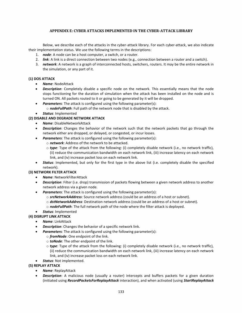
133

APPENDIX E: CYBER ATTACKS IMPLEMENTED IN THE CYBER-ATTACK LIBRARY

Below, we describe each of the attacks in the cyber-attack library. For each cyber-attack, we also indicate

their implementation status. We use the following terms in the descriptions: 1. node: A node can be a host computer, a switch, or a router. 2. link: A link is a direct connection between two nodes (e.g., connection between a router and a switch). 3. network: A network is a graph of interconnected hosts, switchers, routers. It may be the entire network in

the simulation, or any part of it. (1) DOS ATTACK

Name: NodeAttack

Description: Completely disable a specific node on the network. This essentially means that the node stops functioning for the duration of simulation when the attack has been installed on the node and is turned ON. All packets routed to it or going to be generated by it will be dropped.

Parameters: The attack is configured using the following parameter(s): o nodeFullPath: Full path of the network node that is disabled by the attack.

Status: Implemented (2) DISABLE AND DEGRADE NETWORK ATTACK

Name: DisableNetworkAttack

Description: Changes the behavior of the network such that the network packets that go through the network either are dropped, or delayed, or congested, or incur losses.

Parameters: The attack is configured using the following parameter(s): o network: Address of the network to be attacked. o type: Type of the attack from the following: (i) completely disable network (i.e., no network traffic),

(ii) reduce the communication bandwidth on each network link, (iii) increase latency on each network link, and (iv) increase packet loss on each network link.

Status: Implemented, but only for the first type in the above list (i.e. completely disable the specified network).

(3) NETWORK FILTER ATTACK

Name: NetworkFilterAttack

Description: Filter (i.e. drop) transmission of packets flowing between a given network address to another network address via a given node.

Parameters: The attack is configured using the following parameter(s): o srcNetworkAddress: Source network address (could be an address of a host or subnet). o dstNetworkAddress: Destination network address (could be an address of a host or subnet). o nodeFullPath: The full network path of the node where the filter attack is deployed.

Status: Implemented (4) DISRUPT LINK ATTACK

Name: LinkAttack

Description: Changes the behavior of a specific network link.

Parameters: The attack is configured using the following parameter(s): o fromNode: One endpoint of the link. o toNode: The other endpoint of the link. o type: Type of the attack from the following: (i) completely disable network (i.e., no network traffic),

(ii) reduce the communication bandwidth on each network link, (iii) increase latency on each network link, and (iv) increase packet loss on each network link.

Status: Not implemented. (5) REPLAY ATTACK

Name: ReplayAttack

Description: A malicious node (usually a router) intercepts and buffers packets for a given duration (initiated using RecordPacketsForReplayAttack interaction), and when activated (using StartReplayAttack

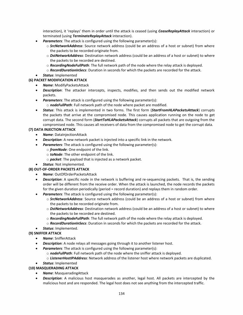
134

interaction), it ‘replays’ them in order until the attack is ceased (using CeaseReplayAttack interaction) or terminated (using TerminateReplayAttack interaction).

Parameters: The attack is configured using the following parameter(s): o SrcNetworkAddress: Source network address (could be an address of a host or subnet) from where

the packets to be recorded originate from. o DstNetworkAddress: Destination network address (could be an address of a host or subnet) to where

the packets to be recorded are destined. o RecordingNodeFullPath: The full network path of the node where the relay attack is deployed. o RecordDurationInSecs: Duration in seconds for which the packets are recorded for the attack.

Status: Implemented (6) PACKET MODIFICATION ATTACK

Name: ModifyPacketsAttack

Description: The attacker intercepts, inspects, modifies, and then sends out the modified network packets.

Parameters: The attack is configured using the following parameter(s): o nodeFullPath: Full network path of the node where packet are modified.

Status: This attack is implemented in two forms. The first form (StartFromHLAPacketsAttack) corrupts the packets that arrive at the compromised node. This causes application running on the node to get corrupt data. The second form (StartToHLAPacketsAttack) corrupts all packets that are outgoing from the compromised node. This causes all receivers of data from the compromised node to get the corrupt data.

(7) DATA INJECTION ATTACK

Name: DataInjectionAttack

Description: A new network packet is injected into a specific link in the network.

Parameters: The attack is configured using the following parameter(s): o fromNode: One endpoint of the link. o toNode: The other endpoint of the link. o packet: The payload that is injected as a network packet.

Status: Not implemented. (8) OUT-OF-ORDER PACKETS ATTACK

Name: OutOfOrderPacketsAttack

Description: A specific node in the network is buffering and re-sequencing packets. That is, the sending order will be different from the receive order. When the attack is launched, the node records the packets for the given duration periodically (period = record duration) and replays them in random order.

Parameters: The attack is configured using the following parameter(s): o SrcNetworkAddress: Source network address (could be an address of a host or subnet) from where

the packets to be recorded originate from. o DstNetworkAddress: Destination network address (could be an address of a host or subnet) to where

the packets to be recorded are destined. o RecordingNodeFullPath: The full network path of the node where the relay attack is deployed. o RecordDurationInSecs: Duration in seconds for which the packets are recorded for the attack.

Status: Implemented. (9) SNIFFER ATTACK

Name: SnifferAttack

Description: A node relays all messages going through it to another listener host.

Parameters: The attack is configured using the following parameter(s): o nodeFullPath: Full network path of the node where the sniffer attack is deployed. o ListenerHostIPAddress: Network address of the listener host where network packets are duplicated.

Status: Implemented (10) MASQUERADING ATTACK

Name: MasqueradingAttack

Description: A malicious host masquerades as another, legal host. All packets are intercepted by the malicious host and are responded. The legal host does not see anything from the intercepted traffic.

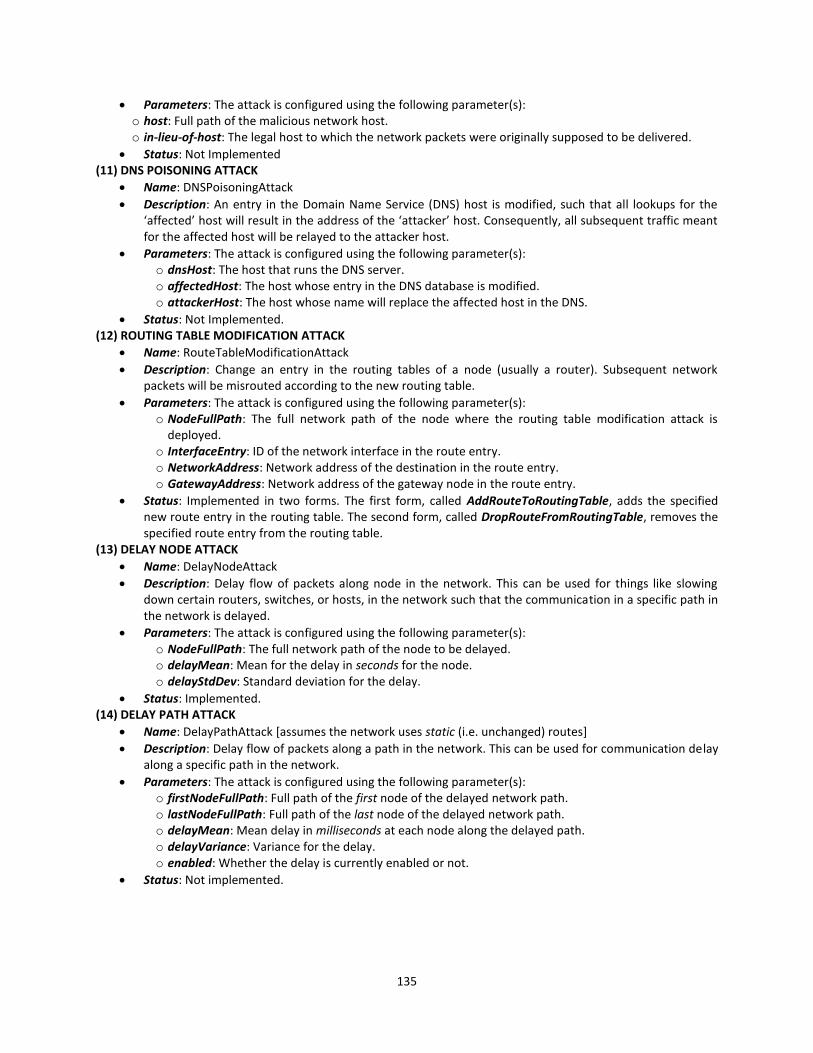
135

Parameters: The attack is configured using the following parameter(s): o host: Full path of the malicious network host. o in-lieu-of-host: The legal host to which the network packets were originally supposed to be delivered.

Status: Not Implemented (11) DNS POISONING ATTACK

Name: DNSPoisoningAttack

Description: An entry in the Domain Name Service (DNS) host is modified, such that all lookups for the ‘affected’ host will result in the address of the ‘attacker’ host. Consequently, all subsequent traffic meant for the affected host will be relayed to the attacker host.

Parameters: The attack is configured using the following parameter(s): o dnsHost: The host that runs the DNS server. o affectedHost: The host whose entry in the DNS database is modified. o attackerHost: The host whose name will replace the affected host in the DNS.

Status: Not Implemented. (12) ROUTING TABLE MODIFICATION ATTACK

Name: RouteTableModificationAttack

Description: Change an entry in the routing tables of a node (usually a router). Subsequent network packets will be misrouted according to the new routing table.

Parameters: The attack is configured using the following parameter(s): o NodeFullPath: The full network path of the node where the routing table modification attack is

deployed. o InterfaceEntry: ID of the network interface in the route entry. o NetworkAddress: Network address of the destination in the route entry. o GatewayAddress: Network address of the gateway node in the route entry.

Status: Implemented in two forms. The first form, called AddRouteToRoutingTable, adds the specified new route entry in the routing table. The second form, called DropRouteFromRoutingTable, removes the specified route entry from the routing table.

(13) DELAY NODE ATTACK

Name: DelayNodeAttack

Description: Delay flow of packets along node in the network. This can be used for things like slowing down certain routers, switches, or hosts, in the network such that the communication in a specific path in the network is delayed.

Parameters: The attack is configured using the following parameter(s): o NodeFullPath: The full network path of the node to be delayed. o delayMean: Mean for the delay in seconds for the node. o delayStdDev: Standard deviation for the delay.

Status: Implemented. (14) DELAY PATH ATTACK

Name: DelayPathAttack [assumes the network uses static (i.e. unchanged) routes]

Description: Delay flow of packets along a path in the network. This can be used for communication delay along a specific path in the network.

Parameters: The attack is configured using the following parameter(s): o firstNodeFullPath: Full path of the first node of the delayed network path. o lastNodeFullPath: Full path of the last node of the delayed network path. o delayMean: Mean delay in milliseconds at each node along the delayed path. o delayVariance: Variance for the delay. o enabled: Whether the delay is currently enabled or not.

Status: Not implemented.

136

REFERENCES

1. J. Sztipanovits, Composition of cyber-physical systems, in Proc. of the 14th Annual IEEE Int’l. Conference and Workshops on the Engineering of Computer-Based Systems (ECBS ’07). Washington, DC, USA: IEEE Computer Society, 2007, pp. 3–6.

2. F. Hassel, P. L. Marrec, C. Valderrama, M. Romdhani, and A. A. Jerraya, MCI: Multilanguage Distributed Cosimulation Tool, in F. J. Ramming (ed.), Distributed and Parallel Embedded Systems, Kluwer Academic Publishers, 1999, (Proceedings of DIPES 98).

3. K. Kim, Y. Kim, Y. Shin, and K. Choi, An Integrated Hardware-Software Cosimulation Environment with Automated Interface Generation, in 7th International Workshop on Rapid Systems Prototyping, June 1996.

4. Functional Mock-up Interface – www.fmi-standard.org 5. T. Blochwitz, M. Otter, M. Arnold, C. Bausch, C. Clauß, H.Elmqvist, A. Junghanns, J. Mauss, M. Monteiro, T.

Neidhold, D. Neumerkel, H. Olsson, J. V. Peetz, S. Wolf, The Functional Mockup Interface for Tool Independent Exchange of Simulation Models, in 8th International Modelica Conference, Dresden, 2011, pp. 20-22.

6. Modelica Association: Modelica – A Unified Object-Oriented Language for Physical Systems Modeling. Language Specification, Version 3.2, March 24, 2010: www.modelica.org/documentas/ModelicaSpec32.pdf

7. Gerardo Pardo-Castellote, OMG Data Distribution Service: Architectural overview, IEEE International Conference on Distributed Computing Systems, 2003.

8. OMG: Data Distribution Service for Real-Time Systems RFP, Document orbos/2003-03-15, http://www.omg.org, March 2003.

9. R. Joshi and G. Castellote, A comparison and mapping of data distribution service and high-level architecture, Real-Time Innovations, Research Program, Washington, DC, 2004.

10. N. Wang, D. Schmidt, H. Hag, and A. Corsaro, Toward an adaptive data distribution service for dynamic large-scale network-centric operation and warfare (NCOW) systems, in Proc. IEEE Military Communications Conference MILCOM, 2008, pp. 1-7.

11. D. Kim, O. Paek, T. Lee, S. Park and H. Bae, A DDS-based distributed simulation approach for engineering-level models, Proceedings of the Winter Simulation Conference 2014, Savanah, GA, 2014, pp. 2919-2930. doi: 10.1109/WSC.2014.7020132.

12. SIMNET – Simulation Network Protocol, https://en.wikipedia.org/wiki/SIMNET 13. RPR-FOM 2.0 – SISO-STD-001.1-2015: Standard for Real-time Platform Reference Federation Object Model

(RPR FOM), Version 2.0 (10 Aug 2015). 14. IEEE 1278.1-2012 - Standard for Distributed Interactive Simulation - Application protocols. 15. TENA – Test and Training Enabling Architecture, www.tena-sda.org 16. CORBA Component Model (CCM) - http://www.omg.org/spec/CCM/ 17. The ACE Orb (TAO) – http://www.cs.wustl.edu/~schmidt/ACE-overview.html 18. SISO-STD-004-2004: Standard for Dynamic Link Compatible HLA API Standard for the HLA Interface

Specification (v1.3) (reaffirmed 8 Dec 2014). 19. US Department of Defense, DMSO, High Level Architecture Interface Specification, v1.3, April 2, 1998. 20. IEEE Std 1516TM-2010. IEEE standard for modeling and simulation (M&S) high-level architecture (HLA) —

Framework and rules. 2010. 21. Portico RTI – http://portico.openlvc.org 22. Pitch RTI – http://www.pitchtechnologies.com/products/prti/ 23. Mak RTI – http://www.mak.com/products/link/mak-rti 24. The JGroups Project - http://jgroups.org/ 25. WebLVC – SISO-REF-051-2014: WebLVC Study Group Final Report. 26. Peter Fritzson, Peter Aronsson, Håkan Lundvall, Kaj Nyström, Adrian Pop, Levon Saldamli, and David Broman.

The OpenModelica Modeling, Simulation, and Software Development Environment, Simulation News Europe, 44(45), December 2005.

27. Dymola – Dynamic Modeling Laboratory, http://www.3ds.com/products-services/catia/products/dymola/ 28. MATLAB/Simulink – http://www.mathworks.com

137

29. Schütte, Steffen, Stefan Scherfke, and Michael Sonnenschein. "Mosaik-smart grid simulation api." Proceedings of SMARTGREENS (2012): 14-24.

30. SimPy – Discrete Event Simulation in Python, http://simpy.readthedocs.org/ 31. The Ptolemy Project – http://ptolemy.eecs.berkeley.edu/ 32. G. Lasnier, J. Cardoso, P. Siron, C. Pagetti, and P. Derler, Distributed simulation of heterogeneous and real-time

systems, in Distributed Simulation and Real Time Applications (DS-RT), 2013 IEEE/ACM 17th International Symposium on, Oct 2013, pp. 55-62.

33. Selim Ciraci, Jeff Daily, Jason Fuller, Andrew Fisher, Laurentiu Marinovici, and Khushbu Agarwal. 2014. FNCS: a framework for power system and communication networks co-simulation. In Proceedings of the Symposium on Theory of Modeling & Simulation - DEVS Integrative (DEVS '14). Society for Computer Simulation International, San Diego, CA, USA, Article 36, 8 pages.

34. ZeroMQ – Decentralized messaging framework, http://zeromq.org/ 35. GridLAB-D – Power distribution simulator, http://www.gridlabd.org/ 36. EnergyPlus – Building energy simulator, http://apps1.eere.energy.gov/buildings/energyplus/ 37. ns-3 – Discrete event network simulator, https://www.nsnam.org/ 38. Karsai, G., Lang, A., Neema, S., Tool Integration Patterns, Workshop on Tool Integration in System

Development. In: ESEC/FSE, Helsinki, Finland, September 2003, pp. 33–38 (2003). 39. B. P. Zeigler and H. S. Sarjoughian, Introduction to DEVS Modeling and Simulation with JAVA: Developing

Component-based Simulation Models, Technical report, 2003. 40. C. Siaterlis, B. Genge, and M. Hohenadel, Epic: A testbed for scientifically rigorous cyber-physical security

experimentation, Emerging Topics in Computing, IEEE Transactions on, vol. 1, pp. 319–330, Dec 2013. 41. B. White, An integrated experimental environment for distributed systems and networks, Proc. 5th Symp.

Operating Syst. Design Implement, pp. 255-270, 2002. 42. Oberle, D., Guarino, N., & Staab, S., What is an ontology? In: "Handbook on Ontologies". Springer, 2nd edition,

2009. 43. Gangemi A., Presutti V., Ontology Design Patterns. In Staab S. et al. (eds.): Handbook on Ontologies (2nd

edition), Springer, 2009. 44. Movshovitz-Attias, Dana and Cohen, William W. Bootstrapping Biomedical Ontologies for Scientific Text using

NELL, BioNLP in NAACL, Association for Computational Linguistics, 2012. 45. A. Marchetti et al., Formalizing Knowledge by Ontologies: OWL and KIF, IIT, CNR, 2008. 46. W3C Semantic Web - http://www.w3.org/standards/semanticweb/ 47. Resource Description Framework - https://www.w3.org/RDF/ 48. Web Ontology Language (OWL) - https://www.w3.org/OWL/ 49. DARPA Agent Markup Language (DAML) – http://www.csl.sri.com/projects/daml/ 50. Protégé open-source ontology editor and framework - http://protege.stanford.edu/ 51. The OWL Guide - http://www.w3.org/TR/owl-guide/ 52. JENA Ontology API - https://jena.apache.org/documentation/ontology/ 53. A Semantic Web Rule Language for combining OWL and RuleML - http://www.w3.org/Submission/SWRL/ 54. Gio Wiederhold, An algebra for ontology composition, In Proceedings of 1994 Monterey Workshop on Formal

Methods, pages 56–61, U.S. Naval Postgraduate School, Monterey CA, Sep. 1994. 55. Vei-Chung Liang and Chris Paredis, A Port Ontology for Automated Model Composition, Winter Simulation

Conference, New Orleans, LA, 2003. 56. Miller, J.A., G. T. Baramidze, P.A. Fishwick, and A.P. Sheth, Investigating Ontologies for Simulation Modeling,

Proceedings of the 37th Annual Simulation Symposium, Arlington, VA, April 2004, pp. 55-71. 57. Lacy, Lee, Interchanging Discrete Event Simulation: Process Interaction Models using The Web Ontology

Language - OWL. Electronic Theses and Dissertations. Paper 1017. http://stars.library.ucf.edu/etd/1017. 58. Benjamin, P., K. Akella, and A. Verma. 2007, Using ontologies for simulation integration, In Proceedings of the

Winter Simulation Conference, 1081–1089. Washington, DC: IEEE Computer Society. 59. Rahman, M. A., Pakstas, A., and Wang, F. Z., CNMO: Towards the Construction of a Communication Network

Modelling Ontology, In Springer book, Intelligent Engineering Systems and Computational Cybernetics, 2009, pp. 143-159, ISBN 978-1-4020-8678-6, doi=10.1007/978-1-4020-8678-6_13.

60. Pahl, Claus, Ontology-Based Composition and Transformation for Model-Driven Service Architecture, In Springer book, Model Driven Architecture -- Foundations and Applications: Second European Conference,

138

ECMDA-FA 2006, Bilbao, Spain, July 10-13, 2006. Proceedings, pp. 198--212, ISBN 978-3-540-35910-4, doi=10.1007/11787044_16.

61. J. Mark Pullen and Vincent P. Laviano, A Selectively Reliable Transport Protocol For Distributed Interactive Simulation, 13th DIS Workshop on Standards for the Interoperability of Distributed Simulations, September 1995, paper 95-13-10.

62. Hemingway G, Neema H, Nine H, Sztipanovits J and Karsai G., Rapid synthesis of high-level architecture-based heterogeneous simulation: a model-based integration approach, Simulation 2012; 88(2): 217–232.

63. Neema, H., Lattmann, Z., Bapty, T., Sztipanovits, J., Karsai, G., Neema, S., Gohl, J., Batteh, J., Tummescheit, H., Sureshkumar, C., Model-based integration platform for FMI co-simulation and heterogeneous simulations of cyber-physical systems, In proceedings of the 10th International Modelica Conference, pp. 235-245 (2014).

64. Kreutzer, W., Systems Simulation: Programming Styles and Languages, Wokingham, England: Addison-Wesley, 1986.

65. Simple Object Access Protocol (SOA) - https://en.wikipedia.org/wiki/SOAP 66. K. Jensen, L. M. Kristensen, and L. Wells, Coloured Petri Nets and CPN Tools for modelling and validation of

concurrent systems, International Journal on Software Tools for Technology Transfer 9.3-4 (2007): 213-254. 67. Matlab/Simulink: Multi-domain dynamics simulation tool. http://www.mathworks.com/products/simulink. 68. A. Varga, The OMNeT++ discrete event simulation system, Proceedings of the European simulation

multiconference (ESM’ 2001). Vol. 9. No. S 185. sn, 2001. 69. B. White, J. Lepreau, L. Stoller, R. Ricci, S. Guruprasad, M. Newbold, M. Hibler, C. Barb, and A. Joglekar. An

Integrated Experimental Environment for Distributed Systems and Networks, In Proc. of the Fifth Symposium on Operating Systems Design and Implementation, pages 255–270, Boston, MA, Dec. 2002.

70. Bruno G., Model Based Software Engineering, Chapman & Hall, 1995. 71. The Model-Driven Architecture: http://www.omg.org/mda/, OMG, Needham, MA, 2002. 72. Kalyan S. Perumalla, Parallel and distributed simulation: traditional techniques and recent advances,

Proceedings of the 38th conference on Winter simulation, December 03-06, 2006, Monterey, California. 73. D. C. Karnopp, D. Margolis, and R. Rosenberg, System Dynamics: Modeling and Simulation of Mechatronic

Systems, 4th ed. New Jersey: John Wiley & Sons Inc., 2006. 74. Lee, E., Sabgiovanni-Vincentelli, A. Comparing models of computation. In International Conference on

Computer-Aided Design (ICCAD) (San Jose, California, USA, 1996), ACM/IEEE Computer Society, pp. 234–241. 75. Lee, E., Messerschmitt, D., Synchronous data flow. Proceedings of the IEEE 75, 9 (September 1987), 1235–

1245. 76. Lee, E., Parks, T., Dataflow process networks. Proceedings of the IEEE 83, 5 (May 1995), 773–801. 77. OPNET Network Simulator: https://www.riverbed.com/products/steelcentral/opnet.html 78. Bob Lantz, Brandon Heller, and Nick McKeown. A Network in a Laptop: Rapid Prototyping for Software-Defined

Networks, 9th ACM Workshop on Hot Topics in Networks, October 20-21, 2010, Monterey, CA. 79. D. Harel, Statecharts: A Visual Formalism for Complex Systems, Science of Computer Programming, 1987. 80. IBM Rational Rhapsody: http://www-03.ibm.com/software/products/en/ratirhapfami 81. Network Time Protocol: https://en.wikipedia.org/wiki/Network_Time_Protocol 82. MATLAB Simscape Library: https://www.mathworks.com/help/physmod/simscape/index.html 83. R. M. Fujimoto, Time management in the high-level architecture, Simulation, Dec. 1998. 84. Elias Weingärtner, Florian Schmidt, Hendrik Vom Lehn, Tobias Heer, Klaus Wehrle, SliceTime: a platform for

scalable and accurate network emulation, Proceedings of the 8th USENIX conference on Networked systems design and implementation, March 30-April 01, 2011, Boston, MA.

85. G. S. Ladde and M. Sambandham, Stochastic Versus Deterministic Systems of Differential Equations, Marcel Dekker, New York, 2003.

86. Lamport, L., Time, clocks, and the ordering of events in a distributed system, in Communications of the ACM 21 (7): 558–565. doi:10.1145/359545.359563.

87. ALSP: https://en.wikipedia.org/wiki/Aggregate_Level_Simulation_Protocol 88. R. Bednar and R. E. Crosbie, Stability of multi-rate simulation algorithms, In Proceedings of the 2007 Summer

Computer Simulation Conference (SCSC'07). Society for Computer Simulation International, San Diego, CA, USA, 189-194.

139

89. S.D. Pekarek, O. Wasynczuk, E.A. Walters, J.V. Jatskevich, C.E. Lucas, Ning Wu, P.T. Lamm, An efficient multi-rate simulation technique for power-electronic-based systems, IEEE Trans. Power Syst., vol. 19, no. 1, pp. 399–409, Feb. 2004.

90. S. Narayan, Y. Shi, TCP/UDP network performance analysis of windows operating systems with IPv4 and IPv6, Proceedings of the 2nd IEEE International Conference on Signal Processing Systems (ICSPS), vol. 2, pp. 219-222, 2010, July.

91. Guri, Mordechai, Yosef Solewicz, Andrey Daidakulov, and Yuval Elovici, DiskFiltration: Data Exfiltration from Speakerless Air-Gapped Computers via Covert Hard Drive Noise, arXiv preprint arXiv:1608.03431 (2016).

92. Sturton, Cynthia, Matthew Hicks, David Wagner, and Samuel T. King, Defeating UCI: Building stealthy and malicious hardware, In 2011 IEEE Symposium on Security and Privacy, pp. 64-77. IEEE, 2011.

93. Pierluigi Paganini, Hardware attacks, backdoors and electronic component qualification, Hacking, Oct. 11, 2013 - http://resources.infosecinstitute.com/hardware-attacks-backdoors-and-electronic-component-qualification

94. Rahm, Erhard, and Philip A. Bernstein, A survey of approaches to automatic schema matching, the VLDB Journal 10, no. 4 (2001): 334-350.

95. E. Lee, Cyber physical systems: Design challenges, in Proc. of the 11th IEEE Int’l. Symposium on Object Oriented Real-Time Distributed Computing (ISORC’08), May 2008, pp. 363–369.

96. Awais, M.U., Palensky, P., Elsheikh, A., Widl, E., Matthias, S., The high level architecture RTI as a master to the functional mock-up interface components, Computing, Networking and Communications (ICNC), 2013 International Conference on , vol., no., pp.315,320, 28-31 Jan. 2013. doi: 10.1109/ICCNC.2013.6504102.

97. C2WT community wiki – http://wiki.isis.vanderbilt.edu/OpenC2WT. 98. Sztipanovits, J., and Karsai, G. 1997, Model-Integrated Computing, IEEE Computer, 30(110-112). 99. de Laura, J., and Vangheluwe, H., 2002, AToM3: A Tool for Multi-formalism and Meta-Modeling, Lecture Notes

in Computer Science, 2306 (174-188). 100. Tolvanen, J.P., and Lyytinen, K. 1993, Flexible Method Adaptation in CASE. The Metamodeling Approach,

Scandinavian Journal of Information Science, v5 n1 (71-77). 101. Cook, S., Jones, G., Kent, S., and Wills, A. 2007, Domain-specific Development with Visual Studio DSL Tools,

Addison-Wesley Professional. 102. The Eclipse Foundation – www.eclipse.org 103. Modelon, Inc. – www.modelon.com. 104. JFMI: A Java wrapper for the Functional Mockup Interface – www.ptolemy.eecs.berkeley.edu/java/jfmi. 105. DARPA Adaptive Vehicle Make Program –

www.darpa.mil/Our_Work/TTO/Programs/Adaptive_Vehicle_Make__(AVM).aspx. 106. C. Brooks, E. A. Lee, M. Wetter, T. S. Nouidui, D. Broman, and S. Tripakis. (2012). JFMI - A Java Wrapper for the

Functional Mock-up Interface. Available: http://ptolemy.eecs.berkeley.edu/java/jfmi/ 107. F. Kuhl, R. Weatherly, and J. Dahmann, Creating computer simulation systems: an introduction to the high level

architecture. Prentice Hall PTR Upper Saddle River, NJ, USA, 1999. 108. DEVSJAVA: DEVS Simulator in Java - https://acims.asu.edu/software/devsjava/. 109. D. Krajzewicz, J. Erdmann, M. Behrisch, and L. Bieker, Recent development and applications of SUMO -

Simulation of Urban MObility, International Journal On Advances in Systems and Measurements, vol. 5, no. 3&4, pp. 128–138, December 2012.

110. Delta3D: open-source gaming engine - https://github.com/delta3d/delta3d. 111. TrainDirector: railway traffic control simulation - http://www.backerstreet.com/traindir/en/trdireng.php. 112. HLA Toolbox: https://www.mathworks.com/products/connections/product_detail/product_35843.html. 113. UML – Unified Modeling Language, The Object Management Group - http://www.uml.org. 114. Google Earth – http://www.google.com/earth. 115. Westergaard M., The BRITNeY Suite: A Platform for Experiments, In: Proceedings of 7th Workshop on Practical

Use of Coloured Petri Nets and the CPN Tools, 2006. 116. MySQL Open-Source Database - http://www.mysql.com/. 117. BeagleBone Black Embedded Board - https://beagleboard.org/black. 118. OpenFlow Networking Foundation - https://www.opennetworking.org/. 119. Google Protocol Buffers - http://developers.google.com/protocol-buffers. 120. INET Framework - https://inet.omnetpp.org/. 121. R. Langner, Stuxnet: Dissecting a cyberwarfare weapon, IEEE Security & Privacy, vol. 9, no. 3, pp. 49–51, 2011.

140

122. J. Slay and M. Miller, Lessons learned from the Maroochy water breach, Critical Infrastructure Protection, pp. 73–82, 2007.

123. Business Process Modeling Notation (BPMN) – http://www.bpmn.org/ 124. JGraphX: Java Swing Diagramming Library - https://github.com/jgraph/jgraphx/. 125. Thomas P. Roth, Yuyin Song, Martin J. Burns, Himanshu Neema, William Emfinger, Janos Sztipanovits, Cyber-

physical system development environment for energy applications, 2017 Proceedings of the ASME 2017 11th International Conference on Energy Sustainability (ES2017), Charlotte, NC, June 2017.

126. Mote Carlo Simulation, https://en.wikipedia.org/wiki/Monte_Carlo_method. 127. Role-based access control, https://en.wikipedia.org/wiki/Role-based_access_control. 128. Pacifica Crisis Scenario, January 2002, www.globalsecurity.org/military/library/report/1998/ex2/index.html. 129. Wrenn R., Nagel A., Owens R., Yao D., Neema H., Shi F., Smyth K., van Buskirk C., Porter J., Bapty T., Neema S.,

Sztipanovits J., Ceisel J., Mavris D., Towards Automated Exploration and Assembly of Vehicle Design Models. In ASME 2012 International Design Engineering Technical Conferences and Computers and Information in Engineering Conference (IDETC '2012), Chicago, Illinois, USA, August 12-15, 2012. Volume 2: 32nd Computers and Information in Engineering Conference, Parts A and B, pp. 1143-1152. doi:10.1115/DETC2012-71464.

130. H. Neema, J. Sztipanovits, M. Burns, and E. Griffor, C2WT-TE: A Model-Based Open Platform for Integrated Simulations of Transactive Smart Grids, 2016 Workshop on Modeling and Simulation of Cyber-Physical Energy Systems, Vienna, Austria, 04/2016.

131. C2WT-TE Web-based Integrated Simulation Platform on CPS-VO, http://cps-vo.org/group/C2WTTE. 132. Universal CPS Environment for Federation (UCEF), https://github.com/usnistgov/ucef. 133. Koutsoukos, X., Karsai, G., Laszka, A., Neema, H., Potteiger, P., Volgyesi, P., Vorobeychik, Y., and Sztipanovits,

J., SURE: A Modeling and Simulation Integration Platform for Evaluation of SecUre and REsilient Cyber-Physical Systems, Proceedings of IEEE: IEEE, 2017.

134. H. Neema, P. Volgyesi, B. Potteiger, W. Emfinger, X. Koutsoukos, G. Karsai, Y. Vorobeychik, and J. Sztipanovits, SURE: An experimentation and evaluation testbed for CPS security and resilience: Demo abstract, in Proceedings of the 7th ACM/IEEE International Conference on Cyber-Physical Systems (ICCPS 2016), 2016.

135. Lee, K. H., Hong, J. H. and Kim, T. G. (2015), System of Systems Approach to Formal Modeling of CPS for Simulation-Based Analysis. ETRI Journal, 37: 175–185. doi:10.4218/etrij.15.0114.0863.

136. Distributed Denial of Service (DDoS) attack: https://en.wikipedia.org/wiki/Denial-of-service_attack.