Latin Hyper-Rectangle Sampling for Computer Experiments

David MeaseDepartment of Marketing and Decision Sciences

San Jose State UniversitySan Jose, CA 95192-0069

mease d@cob.sjsu.edu

Derek BinghamDepartment of Statistics and Actuarial Science

Simon Fraser UniversityBurnaby, BC, CANADA V5A 1S6

dbingham@cs.sfu.ca

Abstract

Latin hypercube sampling is a popular method for evaluating the expectation of func-

tions in computer experiments. However, when the expectation of interest is taken with

respect to a non-uniform distribution, the usual transformation to the probability space can

cause relatively smooth functions to become extremely variable in areas of low probability.

Consequently, the equal probability cells inherent in hypercube methods often tend to sam-

ple an insufficient proportion of the total points in these areas. In this paper we introduce

Latin hyper-rectangle sampling to address this problem. Latin hyper-rectangle sampling is

a generalization of Latin hypercube sampling which allows for non-equal cell probabilities.

A number of examples are given illustrating the improvement of the proposed methodology

over Latin hypercube sampling with respect to the variance of the resulting estimators. Ex-

tensions to orthogonal-array based Latin hypercube sampling, stratified Latin hypercube

sampling and scrambled nets are also described.

KEY WORDS: Computer integration; Latin hypercube; Random field.

1 Introduction

The design and analysis of experiments is an important tool used in scientific investigation.

The rapid growth in computer power has made the simulation of complex physical systems

1

more feasible, thereby avoiding costly physical experimentation. Applications range from the

study of prosthetic devices for joint replacement (Chang et. al. 2001) to helicopter rotor design

(Booker et. al. 1997) to the study of hydrocarbon reservoirs in the oil industry (Craig et. al.

1997).

Recent work on the design and analysis of computer experiments includes experiments in

which the goal is to fit a response surface or to optimize a process (e.g., see Santner, Williams

and Notz 2003, for an overview). In these cases, the experiment plans are frequently based

on some variation of Latin hypercube designs (McKay, Conover and Beckman 1979) which

attempt to uniformly fill the input space. Furthermore, it is common to model the outputs

using a spatial process (Sacks et. al. 1989). Under such a model, the output of the simulator

is viewed as a realization of a stochastic process allowing for estimates of uncertainty in a

deterministic computer simulation.

In this article we consider the related problem of estimating the mean of a process. That is,

we are interested in finding the expectation of an unknown function with respect to a known

distribution, where the unknown function is the output of a computer code. This problem

arises in a broad variety of fields such as finance (Caflisch, Morokoff and Owen 1997) and semi-

conductor manufacturing (Kersch, Morokoff and Schuster 1994). In Section 6 we consider

an example dealing with estimating the mean flow of water through a borehole with respect

to randomly distributed borehole dynamics in which water flow is the output of a computer

simulation.

Computing the mean of a process amounts to the evaluation of the integral

µ = E[g(X)] =∫

g(x)f(x)dx, (1)

where f is the known density of the d-dimensional random input vector X = (X1, ..., Xd) and

g(x) is the output from the computer code. Depending on the complexity of the computer code,

a single evaluation of the function g may take seconds, minutes, hours or even days (Currin

et. al. 1991). Consequently, there is a need for methods of evaluating the mean in (1) that

can provide precise results using few function calls of g. When the number of function calls,

n, that can be used is large relative to the dimensionality, d, quadrature methods of numeric

integration are often effective (Davis and Rabinowitz 1984). However, when n is small relative

to d, Monte Carlo based methods such as Latin hypercube sampling (LHS) are preferred (e.g.,

Owen 1997). Indeed, considerable attention has been given to the subject of experiment design

and Monte Carlo in recent years (e.g., Hickernell and Hong 1999 and Loh 2003).

LHS was first described in computer experiment methodology by McKay, Conover and

2

Beckman (1979). The three main features of LHS in this setting are (i) if the n sample

inputs are projected onto any one of the d-dimensions, then exactly one observation falls in

each of the n strata (cells); (ii) each of the cells contain equal probability with respect to

the joint density of the input variables; and (iii) the inputs are obtained by stratified random

sampling, maintaining properties (i) and (ii). In this situation it is generally assumed that the

d components of X are independent.

As a result of the LHS approach, the design space (the input space) is partitioned into equal

probability cells, which may have unintended consequences. Equal probability partitioning for

non-uniform distributions has the effect of creating relatively small cells near the mode(s) of

the distribution of X and larger cells in the tails. Therefore, the resulting sample will tend

to place more points near the mode(s) and relatively few in the tails of the distribution. We

shall see that the potentially large variability of the unknown function in these large cells out

in tails can severely negatively impact the efficiency of the estimator of (1).

In this article we introduce a generalization of Latin hypercube sampling that allows for

non-equal cell probabilities with the aim of estimating (1) more efficiently. (If one were also

interested in variance estimation, then g could be replaced by g2 in (1) and combined with the

estimate of the mean to achieve this goal.) To this end, we propose using a random field as a

surrogate for the unknown function to help partition the input space. We begin by motivating

the problem through two examples in the next section. Next, we introduce the methodology

for one-dimensional integration. In Section 4, we adapt the methodology to integration in

more than one dimension, and in Section 5 we show how one can combine the methodology

with other sampling approaches. Section 6 describes a practical application.

2 Motivation

LHS and variations thereof are frequently used as experiment designs to estimate (1). These

approaches begin by partitioning the space into equal probability cells with respect to the

known density. This equal probability partitioning has important consequences on how the

design points are laid out in the design space. When the density, f , is non-uniform, LHS

employs relatively large cells in areas of low probability. For instance, Figure 1 shows a LHS

design with the corresponding cells when X1 and X2 are independent standard normal variables

truncated to [−3, 3]2. Looking at the figure, the cells far from the center are substantially larger

than the cells near the center.

At first this characteristic may not seem problematic since one would, intuitively, like

3

to sample more thoroughly in regions of high probability. However, the potentially large

variability of g in the large outer regions (i.e., large cells) of low probability in the input space

may be transmitted to the variability of the estimator of (1). That is, the size of the cells in

the tails are larger and thus one might, in the absence of prior knowledge about g, expect that

the variability of g would be larger within the larger cells. (Note that when we write of the

variability of g we are referring to the behavior of the function g itself which should not be

confused with the variance of the random variable g(X).)

−3 −2 −1 0 1 2 3

−3

−2

−1

01

23

x1

x 2

Figure 1: A Sample of n = 50 Points Using LHS

This issue has traditionally been overlooked in the literature. A possible reason for this

is that in (1), the density f can be taken to be uniform by the appropriate inverse CDF

transformation, changing the problem of integration with respect to a known density into

the more generic problem of evaluation of the integral∫[0,1]d g∗(u)du, where g∗ = g(F−1).

While this equivalence is mathematically valid, it obscures the statistical problem and hides

information about the known density f and also the behavior of g in the original space.

As a further illustration, consider the simple function of one variable, g(x), in the left

panel of Figure 2. The same function is plotted in the right panel, except the x-axis has

been transformed to F (x) where F is the standard normal CDF truncated to [−3, 3]. In the

4

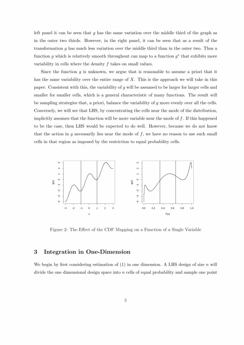
left panel it can be seen that g has the same variation over the middle third of the graph as

in the outer two thirds. However, in the right panel, it can be seen that as a result of the

transformation g has much less variation over the middle third than in the outer two. Thus a

function g which is relatively smooth throughout can map to a function g∗ that exhibits more

variability in cells where the density f takes on small values.

Since the function g is unknown, we argue that is reasonable to assume a priori that it

has the same variability over the entire range of X. This is the approach we will take in this

paper. Consistent with this, the variability of g will be assumed to be larger for larger cells and

smaller for smaller cells, which is a general characteristic of many functions. The result will

be sampling strategies that, a priori, balance the variability of g more evenly over all the cells.

Conversely, we will see that LHS, by concentrating the cells near the mode of the distribution,

implicitly assumes that the function will be more variable near the mode of f . If this happened

to be the case, then LHS would be expected to do well. However, because we do not know

that the action in g necessarily lies near the mode of f , we have no reason to use such small

cells in that region as imposed by the restriction to equal probability cells.

−3 −2 −1 0 1 2 3

−4

−3

−2

−1

01

23

x

g(x)

0.0 0.2 0.4 0.6 0.8 1.0

−4

−3

−2

−1

01

23

F(x)

g(x)

Figure 2: The Effect of the CDF Mapping on a Function of a Single Variable

3 Integration in One-Dimension

We begin by first considering estimation of (1) in one dimension. A LHS design of size n will

divide the one dimensional design space into n cells of equal probability and sample one point

5

in each cell. The estimate of µ is given by

µ̂LHS =n∑

i=1

g(X[i])/n, (2)

where the X[i] are independent random variables for which the distribution is that of X

conditioned on the event that X is in the ith cell.

If instead we wish to allow for non-equal cell probabilities, we can generalize by appropri-

ately re-weighing the terms so that

µ̂ =n∑

i=1

g(X[i])pi, (3)

where pi is the probability of X falling in the ith cell. That is, pi =∫ aiai−1

f(x)dx where the ith

cell (i.e. the ith interval in one dimension) is given by (ai−1, ai] for 1 ≤ i ≤ n, and a0 and an

are taken to be the lower and upper limits of the support of f respectively.

The variance of µ̂ can be written as

Var[µ̂] =n∑

i=1

Var[g(X[i])]p2i . (4)

In order to minimize (4), the conditional variances, Var[g(X[i])], need to be known. Of course,

this cannot be done in practice since the function g is not available to us. Instead, Var[g(X[i])]

is replaced by a model that represents our belief about the general behavior of g. We would

like this model to capture the intuition discussed earlier. That is, because we do not know

where g is most variable, we shall assume that g exhibits the same variability throughout the

support of f , and thus larger cells (i.e. wider intervals) may tend to transmit more variance to

the estimator of (1) than smaller cells. As a result we would expect Var[g(X[i])] to be larger

in larger cells. Further, the more variable the X distribution is within the cell, the larger

Var[g(X[i])] is expected to be.

3.1 Using a Random Field to Determine Non-Equal Probability Cells

In computer experiments, it is common to model g by Gaussian random fields because of the

wide variety of functions they approximate (e.g., Currin et. al. 1991; Welch et. al. 1992). We

will use a random field to make explicit our belief that the variability of g is larger for larger

cells. While the random field model makes the quantity Var[g(X[i])] random, we can use this

property to our advantage.

Here, we make use of the fact that we can compute the expectation of the quantity

Var[g(X[i])] with respect to the random field. Denote the expected variance by Eg(VarX[i][g(X[i])]).

6

For instance, let g be a random field with constant mean. Further assume Var(g(x)− g(y)) is

a function of x− y which we will denote by V (x− y). As a consequence, it can be seen that

Eg(VarX[i](g(X[i]))) =12EX[i],Y [i]V (X[i]− Y [i])

where Y [i] is a second, independent draw from the same distribution as X[i]. Taking V (x, y) =

(x− y)2 gives us

Eg(VarX[i][g(X[i])]) = Var(X[i]).

Since the value of Var(X[i]) is a measure of the dispersion of the random variable X[i],

this formulation directly quantifies the relationship discussed earlier between cell size and

Var[g(X[i])]. That is, Var[g(X[i])] in this formulation is expected to be larger in larger cells.

Furthermore, this approach also quantifies the impact of the variability due to the specific

distribution of X within a cell on the expected value of Var[g(X[i])].

Using this known expectation Eg(Var[g(X[i])]) for each cell now allows us to compute the

expected value of the variance of our estimator µ̂ in (3) over this random field,

n∑

i=1

Var(X[i])p2i . (5)

Ideally, the sampling procedure employed would minimize the variance of our estimator. In

this setting, minimization of (5) is equivalent to minimizing the expected variance of µ̂ with

respect to the specified random field model for g.

The expression in (5) only depends on the cell boundaries ai. Therefore the ai can be

chosen to minimize this expression. To do so, we first rewrite (5) as

n∑

i=1

[si − µ2i ]p

2i , (6)

where the µi are the conditional means of the X[i] (i.e., µi = 1pi

∫ aiai−1

xf(x)dx) and si =

E(X2[i]). Next, we differentiate (6) with respect each ai and set the derivatives equal to zero

to obtain the equations

ai =piµi − pi+1µi+1 +

√(piµi − pi+1µi+1)2 − (pi − pi+1)(pisi − pi+1si+1)

pi − pi+1, (7)

for i ≤ 1 ≤ n− 1.

Since the pi, µi and si are functions of ai−1 and ai, (7) does not give a closed form expression

for the ai. However, (7) suggests the following iterative algorithm.

(1) Initialize a01 < ... < a0

n−1.

7

(2) Using these partitions compute the p0i , µ0

i and s0i for 1 ≤ i ≤ n.

(3) For i ≤ 1 ≤ n− 1 let

a1i =

p0i µ

0i − p0

i+1µ0i+1 +

√(p0

i µ0i − p0

i+1µ0i+1)2 − (p0

i − p0i+1)(p

0i s

0i − p0

i+1s0i+1)

p0i − p0

i+1

(4) Go back to Step 2 using (a11, a

12, ..., a

1n−1) in place of (a0

1, a02, ..., a

0n−1) and iterate until

convergence.

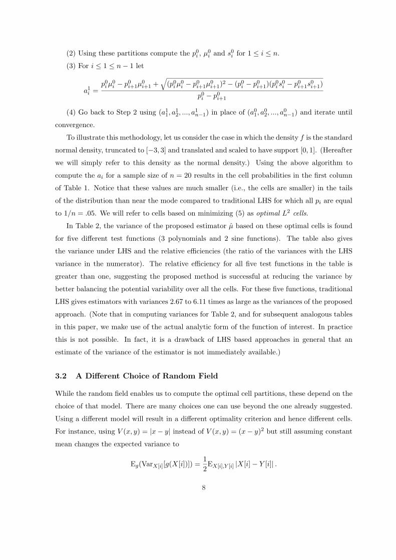
To illustrate this methodology, let us consider the case in which the density f is the standard

normal density, truncated to [−3, 3] and translated and scaled to have support [0, 1]. (Hereafter

we will simply refer to this density as the normal density.) Using the above algorithm to

compute the ai for a sample size of n = 20 results in the cell probabilities in the first column

of Table 1. Notice that these values are much smaller (i.e., the cells are smaller) in the tails

of the distribution than near the mode compared to traditional LHS for which all pi are equal

to 1/n = .05. We will refer to cells based on minimizing (5) as optimal L2 cells.

In Table 2, the variance of the proposed estimator µ̂ based on these optimal cells is found

for five different test functions (3 polynomials and 2 sine functions). The table also gives

the variance under LHS and the relative efficiencies (the ratio of the variances with the LHS

variance in the numerator). The relative efficiency for all five test functions in the table is

greater than one, suggesting the proposed method is successful at reducing the variance by

better balancing the potential variability over all the cells. For these five functions, traditional

LHS gives estimators with variances 2.67 to 6.11 times as large as the variances of the proposed

approach. (Note that in computing variances for Table 2, and for subsequent analogous tables

in this paper, we make use of the actual analytic form of the function of interest. In practice

this is not possible. In fact, it is a drawback of LHS based approaches in general that an

estimate of the variance of the estimator is not immediately available.)

3.2 A Different Choice of Random Field

While the random field enables us to compute the optimal cell partitions, these depend on the

choice of that model. There are many choices one can use beyond the one already suggested.

Using a different model will result in a different optimality criterion and hence different cells.

For instance, using V (x, y) = |x− y| instead of V (x, y) = (x− y)2 but still assuming constant

mean changes the expected variance to

Eg(VarX[i][g(X[i])]) =12EX[i],Y [i] |X[i]− Y [i]| .

8

Normal Exponential Weibull

.015 .097 .278

.028 .092 .151

.038 .087 .110

.046 .082 .086

.053 .077 .070

.058 .072 .058

.062 .067 .048

.065 .062 .040

.067 .057 .033

.068 .052 .028

.068 .048 .023

.067 .043 .019

.065 .038 .015

.062 .033 .012

.058 .028 .009

.053 .023 .007

.046 .018 .005

.038 .013 .003

.028 .008 .002

.015 .003 <.001

Table 1: Optimal L2 Cell Probabilities for Three Distributions

Function Equal Probability Optimal L2 Relative Efficiency

(g(x)) Cells Cells

x 1.76× 10−5 6.31× 10−6 2.80x2 2.54× 10−5 7.46× 10−6 3.40x3 3.84× 10−5 7.71× 10−6 4.99

sin (x) 1.26× 10−5 4.71× 10−6 2.67sin (3x) 1.03× 10−4 1.69× 10−5 6.11

Table 2: L2 Variance Comparison for Five Test Functions for the Normal Distribution

9

The expected variance of g(X[i]) now depends on the L1 measure of dispersion, ∆i ≡EX[i],Y [i]|X[i]−Y [i]|, as opposed to the L2 measure of dispersion, Var(X[i]), from before. The

criterion for choosing the cells now requires minimization of

n∑

i=1

∆ip2i . (8)

Note that if g is Brownian motion, we have V (x, y) ∝ |x − y|. Thus, minimization of (8) is

equivalent to minimizing the expected variance of µ̂ with respect to a Brownian motion model

for g with no drift. As before, we can use this model for g to develop a more efficient estimator

of (1).

Again, we wish to determine the ai to minimize the variance of our estimator. To do this

we differentiate (8) with respect each ai and set the derivatives equal to zero to get

ai =uipi + ui+1pi+1

pi + pi+1; for i ≤ 1 ≤ n− 1. (9)

Since the pi and µi are functions of ai−1 and ai, (9) does not give a closed form expression

for the ai. However, one can use the previous iterative algorithm with (9) replacing (7) in the

third step. We will refer to the resulting cells as the optimal L1 cells.

Using the above algorithm to compute the ai for a sample size of n = 20 for the normal

distribution results in the cell probabilities

(p1, p2, ..., p10) = (p20, p19, ..., p11) = (.026, .037, .044, .049, .053, .055, .057, .059, .060, .060).

Notice that as before these values are smaller in the tails of the distribution than near the

mode compared to traditional LHS. Comparison of the optimal L1 cell probabilities to the

optimal L2 cell probabilities reveals that the L2 solution yields even smaller cells in the tails

of the distribution than the L1 solution.

Table 3 gives the variance of the estimator of (1) based on these optimal L1 cells for the

same five test functions as in Table 2. The results indicate that for these five test functions

the improvement over equal probability cells (LHS) is slightly less substantial. The optimal L1

solution is similar to the optimal L2 solution in that it reduces variance through the reallocation

of sample points to the tails.

3.3 Choice of g

It is important to stress at this time that any reasonable surrogate for g that effectively cap-

tures the notion that g is expected to exhibit more variability over larger, more variable cells

10

Function Equal Probability Optimal L1 Relative Efficiency

(g(x)) Cells Cells

x 1.76× 10−5 7.37× 10−6 2.39x2 2.54× 10−5 9.59× 10−6 2.65x3 3.84× 10−5 1.23× 10−5 3.13

sin (x) 1.26× 10−5 5.39× 10−6 2.33sin (3x) 1.03× 10−4 3.02× 10−5 3.43

Table 3: L1 Variance Comparison for Five Test Functions for the Normal Distribution

will in turn similarly result in smaller cells in the tails of f than LHS. We have illustrated

this for two specific surrogates for g. However, it is possible to entertain a variety of differ-

ent choices for g. Examples of many such models can be found in the computer experiment

literature (Santner, Williams and Notz 2003, Koehler and Owen 1996). Most of the popular

models assume a stationary g and model the covariance between g(x) and g(y) as a function

of |x− y|. The important point is not the specific model that is used, but rather that the par-

titioning is motivated by a model for g which captures the intuition one has and is constructed

independently of the density f . In this paper we are considering the situation in which we

expect g to vary more in larger cells, although in the most extreme case one may even choose a

diffuse surrogate which takes v(x, y) equal to a constant for x 6= y. This reflects a belief that g

varies the same amount over larger cells as it does over smaller cells and reduces the criterion

to minimization of∑n

i=1 p2i for which the equal pi of LHS are optimal. We take the position

that this is too restrictive when one does not have prior knowledge about the behavior of g.

Of course, for any given function g, the improvement in the variance of the estimator over

LHS depends on how well the choice of surrogate reflects the general behavior of the unknown

function. Lastly, we also stress here that regardless of the model for g that is chosen, the

estimator remains unbiased for all g by construction.

These points being made, for the remainder of this paper we will use the L2 cells resulting

from minimization of (5) which correspond to v(x, y) = (x − y)2. This criterion is attractive

for a number of reasons beyond the motivation already presented. First, the criterion can be

motivated without any discussion of a random field model for g by simply supposing that g

satisfies a Lipschitz condition with constant M , i.e.,

|g(x)− g(y)| ≤ M |x− y|

11

for all x and y. In this case the variance of µ̂ is bounded by

M2n∑

i=1

Var(X[i])p2i . (10)

Minimization of this bound corresponds to minimizing (5) and is thus our optimal L2 solution.

Secondly, the criterion given by (5) is equivalent to minimizing the variance for the function

g(x) = x. This makes the criterion simple to compute. Additionally, if we were to approach

the problem by simply choosing a guess for the function g for which to minimize the variance,

the solution would depend on our guess for g only locally through the relationship between the

distribution of X[i] and Var(g(X[i])). This solution assumes that the relationship is equivalent

to that for a function exhibiting predominately linear behavior, which is a reasonable guess

since g is not known. Finally, the L2 criterion is unaffected by the addition of linear drift to

our random field model for g.

Before extending this methodology to the multidimensional case, we will investigate the L2

algorithm through application to two asymmetric distributions: the exponential with a scale

parameter of one and the Weibull with a scale parameter of one and a shape parameter of

1/2. Here we truncate both of these distributions at 100 and again scale so that the support is

[0, 1]. The resulting optimal L2 cell probabilities are displayed in the second and third columns

of Table 1, respectively. The heavy tail behavior of these two distributions results in an even

greater concentration of sampling in the tails, with the Weibull being more extreme than the

exponential.

Tables 4 and 5 compare the variances using the optimal L2 cells to equal probability cells

for the five test functions. The gains in efficiency are more dramatic for these two distributions,

especially for the Weibull. The relative efficiency for the test functions for the Weibull ranges

from 73.76 to 348.26. That is, for g(x) = x2, the variance of the LHS estimator is more than

348 times the variance of the estimator using the proposed approach. Again this is attributable

to the fact that more sampling is done in the long heavy tail of the density f(x), which creates

smaller cells in this part of the distribution than with LHS.

12

Function Equal Probability Optimal L2 Relative Efficiency(g(x)) Cells Cells

x 2.69× 10−7 1.64× 10−8 16.41x2 2.63× 10−9 5.13× 10−11 51.34x3 1.97× 10−11 4.39× 10−13 44.92

sin (x) 2.68× 10−7 1.64× 10−8 16.38sin (3x) 2.37× 10−6 1.47× 10−7 16.15

Table 4: Variance Comparison for the Exponential Distribution for Five Test Functions

Function Equal Probability Optimal L2 Relative Efficiency(g(x)) Cells Cells

x 2.37× 10−5 1.55× 10−7 152.83x2 9.80× 10−6 2.81× 10−8 348.26x3 4.62× 10−6 2.15× 10−8 214.91

sin (x) 2.11× 10−5 1.49× 10−7 141.99sin (3x) 8.52× 10−5 1.16× 10−6 73.76

Table 5: Variance Comparison for the Weibull Distribution for Five Test Functions

3.4 Convergence Issues

At this time, some discussion of the convergence of the algorithms to find the ai is warranted.

In all examples we have studied thus far, the algorithms have always converged, although it

is possible there exist densities for which they may not. In such cases one may need to resort

to other methods for finding the ai to minimize the appropriate expressions, such as a simple

numeric search over a range of values for the ai. Furthermore, even if the algorithm converges,

there is no guarantee that the solution that is found yields the global minimum, unless one

can establish the uniqueness of the solution for the density f of interest. For the L1 solution,

the uniqueness can be established when the density is log-concave. A proof of this uniqueness

result for any log-concave density f is given in the Appendix.

Unlike the L1 solution, the question of whether the concavity of log f(x) (or any condition)

guarantees the uniqueness of a solution to (7) remains open. The problem is closely related

to an optimal partitioning/stratification problem discussed by Eubank (1988) in which the

goal is minimization of∑n

i=1 Var(X[i])pi with respect to the ai. For this problem it is known

that the log-concavity of the density is in fact sufficient for uniqueness (Trushkin 1984). This

differs from our L2 criterion only in that the pi are not squared. Eubank (1988) discusses a

13

number of interesting applications for this related optimal partitioning problem and provides

a slightly weaker sufficient condition for uniqueness than log concavity of the density, although

this condition was later shown to be incorrect by Mease and Nair (2006).

3.5 Relationship with Stratified and Importance Sampling

In this section we discuss some similarities and differences between our sampling/estimation

scheme and standard results in importance sampling and stratified sampling. These two tech-

niques are closely related to our methodology in that they both involve efforts at reduction in

the variance of the basic Monte Carlo estimator by sampling from different input distributions

and reweighting to achieve unbiasedness. There are some key differences, however, as we will

point out.

First consider importance sampling. With this technique, one samples the inputs X[1], ..., X[n]

iid from some distribution with density h and retains unbiasedness in the estimation of µ by

taking the estimator to be

µ̂IS =n∑

i=1

g(X[i])f(X[i])h(X[i])

.

For any given function g the variance of this estimator is minimized by choosing the density h(x)

to be proportional to |g(x)|f(x). This of course is not practical since g is unknown; however,

in practice variance reduction is achieved by using some prior or approximate knowledge of g.

Importance sampling is similar in spirit to our methodology since the estimator is unbiased

for all functions g and is designed to have small variance when the approximate knowledge of

the behavior of g is close to that of the true g. The main difference centers around the way

in which the knowledge is incorporated. While our estimation scheme attempts to balance

variability over all the cells, the importance sampling estimator seeks to sample more heavily

where |g(x)| is expected to be large. Consequently, the optimal importance sampling strategy

is heavily influenced by any knowledge of the actual values of g(x). Conversely, our estimation

scheme does not depend on knowledge of the specific value of g at any point in its domain, but

instead depends on how the variance of g(X) within a cell changes as the cell size is changed.

As an example to contrast the two, let us assume g is Brownian motion with g(0) = ε > 0

and no drift and that f is the uniform density over [−1/2, 1/2]. For this model we noted earlier

that our L1 solution is optimal, which degenerates here to equal probability partitioning since

f is uniform. On the other hand, the optimal importance sampling density which minimizes

the expected variance of the estimator is the density which is proportional to√|x + ε|. Note

that this density relies heavily on the knowledge that g(0) = ε and actually can put arbitrarily

14

small mass at x = 0 if ε is small. In contrast our estimation scheme does not use this knowledge

and is thus invariant with regard to the assumed value of ε. While more elaborate importance

sampling schemes combining the use of control variates may behave differently, this example

serves to illustrate some fundamental differences.

Next we turn to stratified sampling. With stratified sampling one samples ni observations

within the ith stratum such that∑k

i=i ni = n where k is the total number of strata. The ni

observations are sampled iid from the conditional density of f within the ith stratum and we

denote them by X[i, 1], ..., X[i, ni]. The estimator of µ is given by

µ̂Strat =k∑

i=1

ni∑

j=1

g(X[i, j])pi/ni

which has variancek∑

i=1

Var[g(X[i])]p2i /ni (11)

where X[i] refers to a random variable which has a density proportional to the restriction of

f to the ith stratum as before. For any given k ≤ n fixed strata, the variance is minimized

by taking ni ∝ pi

√Var[g(X[i])] which results in a variance of

∑ki=1

√Var[g(X[i])]pi. One can

then choose strata to minimize this quantity. Alternatively, proportional allocation, which

takes ni ∝ pi, is often used. In this case the variance reduces to∑k

i=1 Var[g(X[i])]pi. Choosing

strata to minimize this quantity is the optimal stratification problem mentioned in Section 3.4.

For the one-dimensional case we are currently considering, it is possible to think of our

sampling scheme as a special case of stratified sampling by taking k = n strata and conse-

quently exactly ni = 1 point within each stratum. Note that this is not the standard case in

stratified sampling, as usually the number of strata is fixed to be some value much less than

n. Conversely, in computer experiments one is able to choose the number of cells (strata),

so n cells are used because it is the largest number possible and therefore optimal. It is this

difference that causes the optimal selection of the cell probabilities to differ from both of the

standard optimal stratification problems mentioned above. Specifically, the fact that ni = 1

for all i causes the substitution of ni ∝ pi

√Var[g(X[i])] or ni ∝ pi to not be valid. (Note

these are always just approximate due to the discreetness of the ni, but can be relatively good

approximations when k is much less than n as usually is the case in stratified sampling.) In

our approach, we are instead able to work with an exact expression for the variance by using

the fact that ni = 1 for all i, which caused (11) to reduce to our criterion (4). In the multi-

dimensional case which we will consider next there are additional dissimilarities as a result of

the fact that LHS has a different sampling scheme from standard stratified sampling.

15

4 Integration in More Than One Dimension

In this section we adapt our methodology to more than one dimension (i.e., d > 1). We restrict

attention to independent and identically distributed Xj , j = 1, . . . , d. This assumption allows

for symmetric treatment of the problem in the different dimensions so that the same partitions

are used for each marginal distribution.

To begin, let us first introduce some notation to describe traditional (i.e. equal probability)

LHS. As in one dimension we will let a0, ..., an denote the cell boundaries for each Xj . Since

LHS has equal probability cells, for the time being these are simply the n quantiles for the

common univariate distribution of each Xj . Further let Xj [i] denote the random variable Xj

conditioned on the event that Xj is in (ai−1, ai]. Since the Xj [i] have the same distribution for

all j we can simply use X[i] for the Xj [i]. Finally let D be a n×d (random) matrix formed by

making each column an independent random permutation of the integers 1, ..., n. In this way

the d values in the ith row of the matrix D will give the d univariate cell locations for the ith

point sampled in LHS. Using this notation we can write the estimator from LHS as

µ̂LHS =1n

n∑

i=1

g(X1[D{i, 1}], ..., Xd[D{i, d}]). (12)

Generalizing this to allow for non-equal probability cells is done by simply choosing the

ai to give a non-equal probability partitioning of the marginal distributions. Unbiasedness

can be retained by weighting the points according to the product of the marginal partition

probabilities. Specifically, let the pi be the univariate partition probabilities corresponding to

the ai. That is, pi =∫ aiai−1

f(x)dx where f is the density of the common univariate distribution

of each Xj . Then the estimator is given by

µ̂LHRS =1n

n∑

i=1

g(X1[D{i, 1}], ..., Xd[D{i, d}])ndd∏

j=1

pD{i,j}. (13)

Because the cell probabilities are not necessarily all equal, we call this generalization Latin

hyper-rectangle sampling (LHRS). The rationale is as follows. When viewed in the probability

space, the equal probability partitioning of LHS results in squares in two dimensions, cubes

in three dimensions, and hypercubes in higher dimensions. Conversely, in this space our

non-equal probability partitioning results more generally in rectangles in two dimensions and

hyper-rectangles in higher dimensions.

As in one dimension, in order to find the ai’s that give the partitioning that minimizes the

variance of (13), it is necessary to know the function g. Again, since this is unknown, we will

consider an analog to our treatment of this problem from before.

16

For one dimension, a criterion was motivated that was shown to be equivalent to minimizing

the variance for g(x) = x. For d > 1 a similar LHRS criterion can be motivated by assuming

that g is additive so that g(x) =∑d

i=1 gi(xi). Two analogues of the one-dimensional criterion

then are to minimize the variance for g(x) =∑d

i=1 xi if we believe all dimensions contribute

approximately the same amount to the variability, or to minimize the variance for g(x) = xj

for any xj if we believe one dimension is likely to dominate the others. We will proceed by

using the latter criterion; however, in the examples we examined, the difference in the cells

resulting from the two different criteria is small.

Assuming g(x) = xj for any j (consider j = 1 without loss of generality) we can compute

the variance of (13) as

Var[µ̂LHRS] =1K

K∑

k=1

E(µ̂2LHRS|D = dk)− E2(µ̂LHRS) =

n2d

Kn2

K∑

k=1

n∑

i=1

sip2i

d∏

j=2

pdk{i,j}

2

+ 2n∑

i=1

n∑

m=i+1

µipiµmpm

d∏

j=2

pdk{i,j}d∏

j=2

pdk{m,j}

−E2(µ̂LHRS)

where the dk are the K = n!(d−1) possible D matrices with the rows ordered so that the first

column is the identity permutation. Since E2(µ̂LHRS) does not depend on the ai, it is sufficient

to find the ai to minimize

K∑

k=1

n∑

i=1

sip2i

d∏

j=2

pdk{i,j}

2

+ 2n∑

i=1

n∑

m=i+1

µipiµmpm

d∏

j=2

pdk{i,j}d∏

j=2

pdk{m,j}

∝ E

d∏

j=2

pD{1,j}

2n∑

i=1

sip2i + E

d∏

j=2

pD{1,j}d∏

j=2

pD{2,j}

2

n∑

i=1

n∑

m=i+1

µipiµmpm. (14)

For example, in the simplest nontrivial case n = 2 and d = 2 we see that (14) is given by

s1p21(p

21 + p2

2) + s2p22(p

21 + p2

2) + 4µ1µ2p21p

22. (15)

As in the one dimensional case, in order to choose the ai to minimize (15) we could differentiate

with respect to each ai and solve for the derivative equal to zero. For the present example

we would have only to differentiate with respect to a1 since n = 2 and a0 and an are fixed.

The derivative of (15) with respect to a1 can be written as f(a1)[Aa21 + Ba1 + C] where

A = p31 − p3

2 + p1p22 − p2

1p2, B = 4p1p22µ2 − 4p2

1p2µ1 and C = 3p31s1 + 4µ1µ2p1p

22 − 4µ1µ2p

21p2 −

3s2p32+s1p1p

22−2p2p

21s1+2p1p

22s2−p2

1p2s2. This is set equal to zero by taking the positive root

17

from the quadratic equation. As in the one-dimensional case this does not yield a closed-form

expression for the a1, but an analogous iterative algorithm can be used. For instance, in the

case that X1 and X2 have the standard (non-truncated) exponential distribution, this gives

that the optimal value is a1 = 1.2311, giving p1 = .71 as opposed to p1 = .5 for traditional

LHS. For the function g(x) = x1, the LHRS approach reduces the variance of the estimator

from 0.26 to 0.18, which yields a relative efficiency of 1.4 versus LHS.

While in general this technique of differentiating (14) can be used to obtain quadratic

equations for the partitions that can be solved recursively, for larger n and d these equations

become quite complex and awkward to deal with. The alternative we chose to dealing with

these complex equations was to perform the minimization by simply carrying out a numeric

search over different values of the ai, or equivalently, the pi. Moreover, to compute the value of

the objective variance (14) at each stage of this search we found it more efficient to approximate

the variance of (13) for the function g(x) = x1 through Monte Carlo as opposed to using (14)

directly. This is due to the fact that (14) becomes expensive to compute due to all the possible

combinations for the pi in the products when d > 3.

Our strategy for carrying out this search was as follows. We began by searching over the

values for the pi in the outermost cells equal to the values 0.1/n, 0.2/n, ..., 0.9/n while the other

pi were fixed to be equal and such that∑n

i=1 pi = 1. If one of these values yielded improvement

over the equal probability case, then we searched again over the values 0.1/n, 0.2/n, ..., 0.9/n

for the second partitions from either end, and so on. In this way, we exploited our empirical

observation that the largest differences from equal probability generally occur in the tails of

the distributions.

For the normal distribution in d = 2 dimensions with n = 20 the optimal LHRS partitions

were found to be such that p1 = p20 = 0.9/n with the other pi all equal. The truncated

and scaled exponential distribution from before, not surprisingly, yielded optimal partitions

that differed more from equal probability. These partitions were found to be p20 = 0.5/n,

p19 = 0.8/n and p18 = 0.9/n with the other pi all being equal. The relative efficiencies of

LHRS over LHS for various test functions for these two distributions are given in the second

and third columns of Table 6 respectively (again, with LHS variance in the numerator).

We also searched for optimal pi for the (truncated and scaled) exponential distribution for

d = 3 and d = 8. For d = 3 the optimal pi were found to be p20 = 0.6/n and p19 = 0.9/n

with the other pi all equal. For d = 8 these are closer to equal probability showing the

optimal solution to be p20 = 0.9/n with the other pi equal. This general trend that for a given

18

Function Normal (d = 2) Exponential (d = 2) Exponential (d = 8) Weibull (d = 8)

x1 1.1 1.9 1.1 1.7x2

1 1.1 2.7 1.2 2.5x3

1 1.2 2.5 1.2 2.4sin (x1) 1.2 1.9 1.1 1.6sin (3x1) 1.2 1.8 1.1 1.1∑d

i=1 xi 1.1 1.6 1.1 1.8∑di=1 x2

i 1.1 2.5 1.2 2.4(∑d

i=1 xi)2 1.1 3.1 1.4 3.1x1 × x2 1.1 2.5 1.2 3.0

sin (∑d

i=1 xi) 1.1 1.6 1.1 1.6cos(2

∑di=1 xi) 0.9 3.1 1.4 2.9

exp(−∑di=1 |xi − 1|) 1.1 1.7 1.1 2.4

exp(−∑di=1 |xi − 0|) 1.1 1.5 1.0 1.3

exp(−∑di=1 |xi − 1

2 |) 1.0 1.7 1.1 2.3exp(−∑d

i=1(xi − 1)2) 1.0 1.8 1.2 2.9exp(−∑d

i=1(xi − 0)2) 1.0 2.5 1.2 2.4exp(−∑d

i=1(xi − 12)2) 1.2 1.6 1.1 1.3

Table 6: Relative Efficiencies of LHRS compared to Traditional LHS for 17 Test Functions

19

distribution and fixed n the optimal pi move closer to equal probability as d gets larger was

noticed for other examples as well. However, even for d = 8 the heavy tails of the truncated

and scaled Weibull distribution (defined earlier) yielded optimal pi substantially different from

equal probability, showing p20 = 0.4/n and p19 = 0.9/n. This general trend observed was

that, for a fixed n and d, heavier tails lead to more extreme differences from LHS. Relative

efficiencies of LHRS over LHS for the exponential and Weibull distributions with d = 8 are

given in the fourth and fifth columns of Table 6 respectively.

Of course this simple search algorithm only approximates the optimal solution. One could

derive more accurate, efficient and elegant minimization techniques. However, the technique

used proved to be effective at finding solutions to reduce the variance substantially. More

importantly, the technique can be easily implemented by a practitioner to find the optimal

pi for any given n and d without any special programming except Monte Carlo draws of

the estimator itself. Further, it is practical improvement over equal probability partitioning

that is of interest and not necessarily the location of the global minimum. A more elaborate

search aimed at finding the global minimum may produce diminishing returns depending on

the complexity of the algorithm and the additional variance reduction in the criterion function

that is achieved.

Finally, it is important to point out that unlike in one dimension, with d > 1 the cell prob-

abilities used to weight the points in any single realization of the estimator do not necessarily

sum to one. A consequence of this is that addition or subtraction of a constant term to any

function g(x) will affect the variance of the proposed scheme. In fact, addition or subtraction

of a sufficiently large constant can lead to the proposed scheme having substantially greater

variance than LHS. We have discovered that an extremely effective method of dealing with this

problem is simply to initially subtract off the value of g(x) at the mode of the X distribution

and then add this value back on after the weighing by the cell probabilities is performed. Ac-

cordingly, the same adjustment is made when evaluating the variance for the criterion function

g(x) = x1 to determine the optimal partitions. This was implemented for the test functions

displayed in Table 6 and when determining the optimal partitions given in this section. This

leads to the variance of the LHRS estimator being unaffected by addition or subtraction of

constants and results in the overall general improvement over LHS displayed in Table 6.

20

5 Uniformity in Higher Dimensions

There has been a large amount of research in recent years concerning construction of Latin

hypercube designs that exhibit greater uniformity in two or more dimensions. These are

designs that retain the one-dimensional projection property of LHS, while at the same time

additionally achieve uniformity in more than one dimension. In our notation such designs are

equivalent to placing restrictions on the matrix D in (12). These include orthogonal-array

based Latin hypercubes (Tang 1993; Ye 1998), methods of reducing correlations (Owen 1994),

stratified Latin hypercubes (Lee 1999), and scrambled net designs (Owen 1997).

Adaptation of the methodology presented in this paper is straightforward for such tech-

niques, which, like LHS, are restricted to equal probability cells. The main idea here is to

extend these methods to allow non-equal probability cells and apply the appropriate weighting

to retain the unbiasedness. The criterion used in the previous section can still be applied.

However, the additional uniformity imposed by these techniques will not necessarily lead to

the same optimal cells for a given sample size, dimension, and density function.

As an illustration, we consider an example involving a scrambled net with n = 27 and

d = 3. Specifically this is a (0, 3, 3) scrambled net in base 3. We will take the Xj to be

iid according to the truncated and scaled exponential distribution considered in the previous

section. For LHRS, the optimal cell probabilities using the criterion and search methodology

proposed in the previous section were determined to be p27 = 0.6/n and p26 = 0.9/n with the

other pi all equal. Using this same criterion function, the optimal cell probabilities for the

scrambled net are p27 = 0.6/n and p26 = 0.8/n with the other pi all equal. Figure 3 displays

the two dimensional projections on the probability scale for a realization of a scrambled net

using these values for the pi. The difference from equal probability in the tails can be observed

by noticing that the last two univariate cells on any axis are smaller than the other 25.

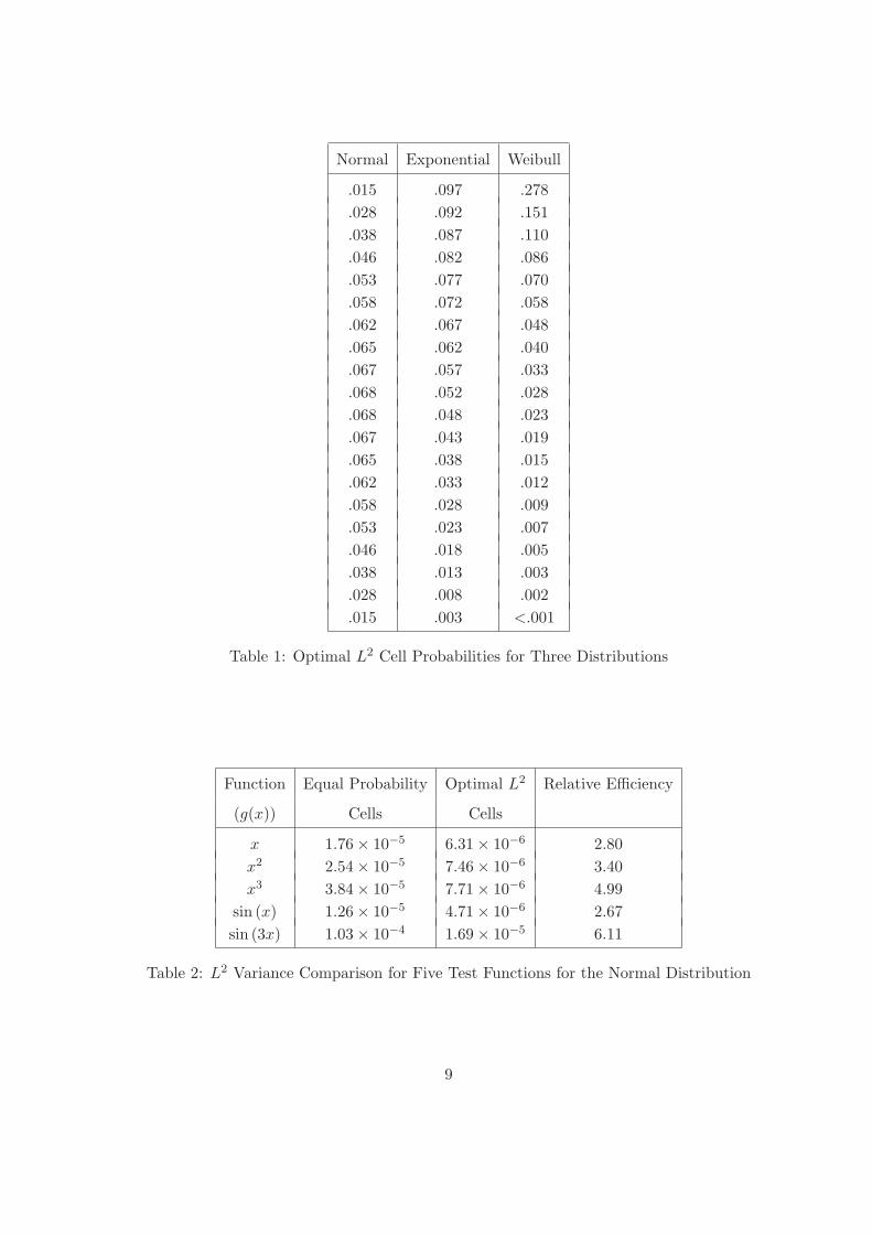
The second column of Table 7 lists the variances for traditional LHS for the various test

functions in the first column. The third column gives the relative efficiency for LHRS using

the optimal cells. The fourth column gives the relative efficiency for the traditional (i.e.

equal probability cell) scrambled net over traditional LHS. The final column gives the relative

efficiency of the LHRS scrambled nets over the variances for the traditional scrambled nets.

From the fourth column of the table it can be seen that scrambled net provides substantial

reduction in variance over the traditional LHS for two of the functions. Columns three and

five show that for both the scrambled net and LHS, the proposed LHRS approach provides

substantial variance reduction over equal probability cells for all of the functions considered.

21

0.0 0.2 0.4 0.6 0.8 1.0

0.0

0.2

0.4

0.6

0.8

1.0

F(x1)

F(x

2)

0.0 0.2 0.4 0.6 0.8 1.0

0.0

0.2

0.4

0.6

0.8

1.0

F(x2)

F(x

3)

0.0 0.2 0.4 0.6 0.8 1.0

0.0

0.2

0.4

0.6

0.8

1.0

F(x1)

F(x

3)

Figure 3: Two Dimensional Projections of a Scrambled Net Using Optimal Partitioning

Note that for all these test functions the improvement resulting from the non-equal probability

cells for scrambled nets is larger or at least as large as for the standard Latin hypercube

approach, as the values in column five are all at least as large as the values in the third column.

This suggests that the proposed methodology benefits even more from the higher dimensional

uniformity imposed by the scrambled net design than do equal probability methods.

6 Example

In this section we apply the LHRS methodology developed in this paper to a particular func-

tion that models a physical phenomenon. The function describes the flow of water through a

22

LHS LHRS Relative Scrambled Net RelativeFunction Variance Efficiency Efficiency Efficiency

x1 1.5× 10−7 1.4 1.0 1.6x2

1 1.6× 10−9 2.0 1.0 2.0x3

1 1.3× 10−11 1.9 1.0 1.9sin (x1) 1.5× 10−7 1.4 1.0 1.6sin (3x1) 1.3× 10−6 1.4 1.0 1.6∑d

i=1 xi 4.4× 10−7 1.3 1.0 1.6∑di=1 x2

i 4.9× 10−9 2.0 1.0 2.0(∑d

i=1 xi)2 1.4× 10−8 2.3 1.3 2.4x1 × x2 4.1× 10−10 1.7 2.6 3.7

sin (∑d

i=1 xi) 4.4× 10−7 1.3 1.0 1.6cos(2

∑di=1 xi) 5.5× 10−8 2.3 1.0 2.4

exp(−∑di=1 |xi − 1|) 1.3× 10−9 1.4 1.0 1.6

exp(−∑di=1 |xi − 0|) 3.9× 10−7 1.2 1.0 1.5

exp(−∑di=1 |xi − 1

2 |) 2.6× 10−8 1.4 1.0 1.6exp(−∑d

i=1(xi − 1)2) 5.3× 10−9 1.5 1.0 1.6exp(−∑d

i=1(xi − 0)2) 4.8× 10−9 2.0 1.0 2.0exp(−∑d

i=1(xi − 12)2) 9.2× 10−8 1.4 1.0 1.5

Table 7: LHS, LHRS and Scrambled Net Variance Comparisons

borehole between two underground aquifers. It was taken from a paper on computer experi-

ments by Morris, Mitchell and Ylvisaker (1993) where the aim was to estimate the response

surface rather than integration. It is important to note that this function differs from the types

of functions typical in computer experiments in the sense that it can be expressed in closed

form and evaluated instantly. However, these qualities are useful for a simulation to evaluate

the effectiveness of our methodology.

The function has d = 8 inputs and is given by

g(x) =2πx3(x4 − x6)

log(x2x1

)[1 + 2x7x3

log(x2/x1)x21x8

+ x3x5

].

The eight inputs x = (x1, ..., x8) are the radius of borehole, the radius of influence, the trans-

missivity of the upper aquifer, the potentiometric head of upper aquifer, the transmissivity of

lower aquifer, the potentiometric head of lower aquifer, the length of borehole and the hydraulic

conductivity of borehole respectively as described by Morris et. al. (1993).

For sake of example, let us suppose that the eight inputs are independent and distributed

according to our truncated and scaled Weibull distribution discussed earlier over their respec-

23

tive ranges. If we estimate (1) with respect to this distribution using a sample size of n = 20

we observe that the LHRS approach yields a relative efficiency of 2.1 over traditional LHS.

7 Concluding Remarks

In this paper we have introduced Latin hyper-rectangle sampling for an important problem in

the design of computer experiments. This technique generalizes traditional LHS to allow for

non-equal probability cells. We have shown that by constructing this partitioning to sample

more points in the tails when the given distribution is non-uniform, practical variance reduction

can be achieved. The benefits of doing this have not previously been realized largely because

the problem is usually considered in the probability space. When combined with variations

on LHS such as scrambled nets, which are aimed at higher dimensional uniformity, additional

gains may be achieved. Indeed, we feel that LHRS is generally preferable to LHS.

We have focused only on the case in which inputs are iid, and it would also be of practical

importance to extend the methodology to treat non-identically distributed inputs as well as

cases in which there exists dependence among the inputs. Further, future work is needed to

consider adapting the methodology to incorporate any specific knowledge about the function

g that might be available. Such information may come from sampling the points sequentially

or from some prior knowledge.

References

Booker, A. J., Dennis, J. E., Frank, P. D., Serafini, D. B. and Torczon, V. (1998), “Optimiza-

tion Using Surrogate Objectives on a Helicopter Test Example,” in Computational Methods in

Optimal Design and Control, 49–58.

Caflisch, R. E., Morokoff, W. J. and Owen, A. B. (1997), “Valuation of Mortgage Backed

Securities using Brownian Bridges to Reduce Effective Dimension,” Journal of Computational

Finance, 1, 27–46.

Chang, P. B., Williams, B. J., Notz, W. I., Santner, T. J. and Bartel, D. L. (1999), “Robust

Optimization of Total Joint Replacements Incorporating Environmental Variables,” Journal

of Biochemical Engineering, 121, 304-310.

24

Craig, P. S., Goldstein, M., Seheult, A. H. and Smith, A. J. (1997), “Pressure Matching for

Hydrocarbon Reservoirs: A Case Study in the use of Bayes Linear Strategies for Large Com-

puter Experiments (with discussion),” in Case studies in Bayesian Statistics, Vol. 3, 36–93,

Oxford University Press.

Currin, C., Mitchell, T. J., Morris, M. D. and Ylvisaker, D. (1991), “Bayesian Prediction of

Deterministic Functions, With Applications to the Design and Analysis of Computer Experi-

ments,” Journal of American Statistical Association, 86, 953-963.

Davis, P. J. and Rabinowitz, P. (1984), Methods of Numerical Integration, New York: Acad-

emic Press.

Eubank, R. L. (1988), “Optimal Grouping, Spacing, Stratification, and Piecewise Constant

Approximation,” SIAM Review, 30, 404-420.

Hickernell, J., and Hong, H. S. (1999), “The Asymptotic Efficiency of Randomized Nets for

Quadrature,” Mathematics of Computation, 68, 767-791.

Kersch, A., Morokoff, W. and Schuster, A. (1994), “Radiative Heat Transfer with Quasi-Monte

Carlo Methods,” Transport Theory and Statistical Physics, 7, 1001-1021.

Koehler, J. and Owen, A. (1996), “Computer experiments,” in Ghosh, S. and Rao, C. R.,

editors, Handbook of Statistics, 13, 261-308, Elsevier Science, New York.

Lee, J. (1999), “Asymptotic Comparison of Latin Hypercube Sampling and its Stratified Ver-

sion,” Journal of the Korean Statistical Society, 28, 135-150.

Loh, W.L. (2003), “On the Asymptotic Distribution of Scrambled Net Quadrature”, Annals

of Statistics, 31, 1282-1324.

McKay, M. D., Conover, W. J. and Beckman, R. J. (1979), “A Comparison of Three Methods

for Selecting Values of Input Variables in the Analysis of Output from a Computer Code,”

Technometrics, 21, 239-245.

25

Mease, D. and Nair, V.N. (2006), “Unique Optimal Partitions of Distributions and Connec-

tions to Hazard Rates and Stochastic Ordering,” Statistica Sinica (to appear).

Morris, M. D., Mitchell, T. J. and Ylvisaker, D. (1993), “Bayesian Design and Analysis of

Computer Experiments: Use of Derivatives in Surface Prediction,” Technometrics, 35, 243-255.

Owen, A. (1994), “Controlling Correlations in Latin Hypercube Samples,” Journal of the

American Statistical Association, 89, 1517-1522.

Owen, A. (1997), “Scrambled Net Variance for Integrals of Smooth Functions,” Annals of Sta-

tistics, 25, 1541-1562.

Sacks, J., Welch, W. J., Mitchell, T. J. and Wynn, H. P. (1989), “Scrambled Net Variance for

Integrals of Smooth Functions,” Annals of Statistics, 25, 1541-1562.

Santner, J. S., Williams, B. J. and Notz, W. I. (2003), The Design and Analysis of Computer

Experiments, Springer, New York.

Shaked, M. and Shanthikumar, J. G. (1994), Stochastic Orders and Their Applications, Boston,

Massachusetts: Academic Press.

Tang, B. (1993), “Orthogonal-Array Based Latin Hypercubes,” Journal of the American Sta-

tistical Association, 88, 1392-1397.

Trushkin, A. (1984), “Monotony of Lloyd’s Method II for Log-Concave Density and Convex

Error Weighting Function,” IEEE Transactions on Information Theory, 30, 380-383.

Welch, W. J., Buck, R. J., Sacks, J., Wynn, H. P., Mitchell, T. J. and Morris, M. D. (1992),

“Screening, Predicting and Computer Experiments,” Technometrics, 34, 15-25.

Ye, K. Q. (1998), “Orthogonal Column Latin Hypercubes and their Applications in Computer

Experiments,” Journal of the American Statistical Association, 93, 1430-1439.

26

Appendix

Proposition: Suppose the density f is equal to a strongly unimodal density f∗ restricted

to an interval (A,B). That is, f(x) = f∗(x) × I[x ∈ (A,B)]/∫ BA f∗(x)dx where log(f∗(x)) is

concave. Then, there exists at most one solution to (9).

Proof: We begin by defining the conditional mean function

u(t, t + h) =∫ t+ht xf∗(x)dx∫ t+ht f∗(x)dx

. (16)

The proof makes repeated use of three results concerning this function.

(I) u(t, t + x) is increasing in x for all t.

(II) u(t− x, t) is decreasing in x for all t.

(III) u(t, t + h)− t is non-increasing in t for all 0 < h ≤ ∞.

Results (I) and (II) follow immediately from the definition of u(·, ·) and the fact that the

density f∗ is strictly positive on (−∞,∞) (because it is log-concave). Result (III) can be found

in the first chapter of Shaked and Shanthikumar (1994).

Now suppose there exist two solutions to (9) given by (aP1 , aP

2 , ..., aPn−1) and (aQ

1 , aQ2 , ..., aQ

n−1).

Let i∗ be the largest i such that aPi 6= aQ

i . Without loss of generality we will take aPi∗ < aQ

i∗ .

Then (II) and (9) with i = i∗ imply aPi∗−1 < aQ

i∗−1. Furthermore, (I) and (III) imply aQi∗−aQ

i∗−1 <

aPi∗ − aP

i∗−1. Using this, (II), (III), and (9) with i = i∗ − 1 give aQi∗ − aQ

i∗−2 < aPi∗ − aP

i∗−2.

From this follows that aPi∗−2 < aQ

i∗−2 and then (I) and (III) with (9) for i = i∗ − 1 give

aQi∗−1−aQ

i∗−2 < aPi∗−1−aP

i∗−2. Continuing inductively in this manner gives for all 1 ≤ i ≤ i∗−1

that aPi < aQ

i and aQi+1 − aQ

i < aPi+1 − aP

i . However, we will eventually have aP2 < aQ

2 along

with aQ2 − aQ

1 < aP2 − aP

1 which is a contradiction of (I),(III) and (9) with i = 1.

Acknowledgments

David Mease’s research was supported by a University of Michigan Rackham Predoctoral Fel-

lowship and an NSF-DMS Postdoctoral Fellowship. Derek Bingham’s research was supported

by a grant from the Natural Sciences and Engineering Council of Canada. We would like to

thank Vijay Nair and the referees for their helpful comments.

27