lattice boltzmann method for simulating impulsive water

Scientia Iranica A (2014) 21(2), 318{328

Sharif University of TechnologyScientia Iranica

Transactions A: Civil Engineeringwww.scientiairanica.com

Lattice Boltzmann method for simulating impulsivewater waves generated by landslides

A. Pak� and M. Sarfaraz

Department of Civil Engineering, Sharif University of Technology, Tehran, P.O. Box 11155-9313, Iran.

Received 6 April 2013; received in revised form 6 July 2013; accepted 27 July 2013

KEYWORDSLattice Boltzmannmethod;Impulsive waterwaves;Landslides;Free surface ow;Numerical modeling.

Abstract. Impulsive water waves generated by landslides impose severe damage oncoastal areas. Very large mass ows in the ocean can generate catastrophic tsunamis.Preventing damage to dams and coastal structures, and saving the lives of local peopleagainst landslide-generated waves, has become an increasingly important issue in recentyears. Numerical modeling of landslide-generated waves is a challenging subject in CFD.The reason lies in the di�culty of determining the interaction between the moving solidsand sea water, which causes complicated turbulent regimes around the moving mass andat the water surface. Submarine or aerial types of landslide can further complicate theproblem. Up to now, a number of numerical approaches have been proposed for predictingthe behavior of ow during and after mass movement. In this study, a Lattice BoltzmannMethod (LBM) based-code is employed for analyzing and simulating the impulsive waterwaves generated by landslides. Four experimental cases of submerged and aerial landslideshave been modeled to investigate the e�ciency and accuracy of the LBM code, and theobtained results are veri�ed against experimental observations. The results indicate thecapability of LBM in simulating complicated ow �elds and demonstrate its superiorityover numerical methods used so far, such as SPH and RANS.c 2014 Sharif University of Technology. All rights reserved.

1. Introduction

Impulsive water waves generated by aerial or sub-merged landslides can exert considerable damage oncoastal areas. These landslides frequently occur indam reservoirs, lakes, and oceans. Saving the livesof local people and reinforcing the structures in theseareas, because of the detrimental e�ects of impulsivewaves, has turned into a major issue for coastalauthorities.

A number of laboratory tests have been conductedto study aerial and submerged landslides, e.g. Hein-rich [1], Walder et al. [2], Fritz et al. [3], Grilli andWatts [4], Panizzo et al. [5], and Ataie and Naja� [6].

*. Corresponding author. Tel.: +98 21 6616 4225E-mail addresses: [email protected] (A. Pak);[email protected] (M. Sarfaraz)

Studies show that a complex nonlinear interactionoccurs between the surface waves and the motion ofthe sliding body.

Until now, two major numerical schemes havebeen utilized to model impulsive waves generated bylandslides. The �rst class contains the conventionalCFD method, founded on solving Navier-Stokes andVOF equations, which is an Eulerian and macroscopicapproach. Rzadkiewicz et al. [7], Titov [8], Imran etal. [9], and Pak and Sarfaraz [10] are some examples ofapplying this method.

This method has some drawbacks when it is usedto simulate the severe interaction between water andsliding material. The VOF scheme adds an additionaltransport equation and an arti�cial di�usion to theinterface pro�le [11]. Coupling uid ow with themoving boundaries of the sliding block is challengingand di�cult using the Eulerian method [12]. Also,

A. Pak and M. Sarfaraz/Scientia Iranica, Transactions A: Civil Engineering 21 (2014) 318{328 319

this method su�ers from instability, extensive compu-tational time and poor scalability [13].

In the second approach, SPH, a macroscopicscheme, is employed to model the motion of thelandslides in water. Due to its Lagrangian scheme,it has been used vastly by researchers in studyinglandslides, e.g. Monaghan and Kos [14], Gotoh etal. [15], Lo and Shao [16], Shao and Lo [17], Shaoand Gotoh [18], Ataie and Shobeyri [19], and Mansour-Rezaei and Ataie [20].

The stability, accuracy, and speed of SPH dependon its smoothing kernel, which should be chosen care-fully for each speci�c problem [13,21]. In particular,a unique kernel function has not been proposed assuitable for all landslide problems, including di�erentgeometrical and physical parameters [19]. Incompress-ibility cannot be strictly assured in commonly usedSPH codes, because, in these codes, a relation betweenpressure and density is assumed [13]. Boundaries arenot modeled well in SPH. The particles at the edgeof the objects have no neighbors outside, so, theirdensities are less than those of internal particles [22].In most of the developed codes, e.g. [19,20,23], SPHwas not used to model the landslide motion through afully-coupled interaction with water, i.e. a prescribedrelation obtained by physical tests was implemented forthe velocity of the solid. Yim et al. [23] reported thatthe accuracy of SPH was less than that of the Eulerianapproach.

Apart from the Eulerian and SPH approaches,the Lattice Boltzmann Method (LBM) has becomepro�cient in solving a variety of complex and di�cult uid dynamic problems over the last 15 years. Thefundamental idea of the LBM is to construct sim-pli�ed kinetic models that incorporate the essentialphysics of microscopic or mesoscopic processes, so thatthe microscopic averaged properties obey the desiredmacroscopic equations [24].

In LBM, the spatial space is discretized in sucha way that it is consistent with the kinetic equa-tion. LBM is a mesoscopic model simulating owphenomenon through tracking uid particle packs thatmove and collide in space under the rules in whichcollision does not result in mass and momentumchanges [25]. Space is divided into regular lattices and,at each lattice site, a particle distribution function, f�,is de�ned, which is equal to the expected number ofparticles of uid in the direction of �. During eachdiscrete time step of the simulation (�t), uid particlesmove to the nearest lattice site along their directionof motion, with di�erent velocities of e�, where they\collide" with other uid particles that arrive at thesame site. The outcome of the collision is determinedby solving the kinetic (Boltzmann) equation for thenew particle distribution function at that site, and theparticle distribution function is updated [24].

LBM has been employed to model complicated ow, such as turbulent and free surface ows, ac-curately [26,27]. The parallelism of the algorithm,simplicity of programming and possibility of modelingcomplex geometrical ow problems are remarkableadvantages of LBM [27]. A single LB time-step issigni�cantly faster than a single step of an Euleriansolver [13]. Hence, time dependent ow modeling isstraightforward, especially in 3D, whereas it is costlyin the Eulerian approach [25]. Also, LBM exhibits goodstability for unsteady problems [27].

This paper aims to simulate impulsive wavesgenerated by aerial and submarine landslides, usingLBM to exhibit its accuracy and e�ciency in modelingthis complicated free-surface problems. According tothe authors' knowledge, this is the �rst research thatuses LBM to simulate the impulsive waves generatedby landslides.

2. Numerical formulation

In this paper, the Single Relaxation Time (SRT) ap-proximation with the Bhantager-Gross-Krook (BGK)collusion rule is adopted to discretize the Boltzmannequation. For the D2Q9 model (Figure 1), it is givenby [28]:

f�(~xi + ~e��t; t+ �t)� f�(~xi; t) =

� f�(~xi; t)� f eq� (~xi; t)

�+ F�; (1)

where xi, e�, �t, f�, f eq� and F� are the position of

the point in the discretized space, the discrete particlevelocity, the time step, the distribution function, thecorresponding equilibrium distribution function andthe body force (e.g. gravity) function, respectively.

Figure 1. D2Q9 lattice scheme.

320 A. Pak and M. Sarfaraz/Scientia Iranica, Transactions A: Civil Engineering 21 (2014) 318{328

To satisfy the incompressible ow limit, according tothe Navier-Stokes equation, by adopting the Chapman-Enskog expansion, the relaxation time (�) is related tothe uid viscosity (�), as [29]:

� =13�� 1

2��t: (2)

The equilibrium distribution is of the form [29]:

f eq� = �!�

�1 + 3 ~e�:~u+ 4:5( ~e�:~u)2 � 1:5~u:~u

�; (3)

where u is the uid velocity, and !� is de�ned as:

!� =

8><>:16=36 � = 04=36 � = 1; 3; 5; 71=36 � = 2; 4; 6; 8

(4)

Gravity vector (g) for free surface modeling is consid-ered as [30]:

F� = 3!��[( ~e� � ~u) + ( ~e�:~u) ~e�]:~g: (5)

Density (�) and momentum uxes (�u) are evaluatedby:

� =8X

�=0

f� =8X

�=0

f eq� ; (6)

�~u =8X

�=0

~e�f� =8X

�=0

~e�f eq� : (7)

For three-dimensional problems in this study, theD3Q19 model was implemented. The reader is referredto [11] for related formulation.

Due to the highly turbulent nature of the ow�eld generated by landslides, it is necessary to use aturbulence model. The role of this procedure is toparameterize the turbulent energy dissipation, wherelarger eddies extract energy from the mean ow andtransfer some of it to smaller eddies [31]. In this paper,the Wall-Adapting Local Eddy-viscosity (WALE), anLES category, is adopted. This model has goodproperties both near to and far from the wall, withlaminar and turbulent ows. This model recovers theasymptotic behavior of the turbulent boundary layerwhen this layer can be directly solved, and it does notadd arti�cial turbulent viscosity in the shear regionsout of the wake. The WALE model is formulatedas [32]:

� = 3�� + C2

t �2��

+0:5; (8)

where Ct is equal to 0:5 and � denotes the �lter

width, which is set to lattice spacing (resolution). �is described as:

� =(gi;jgi;j)1:5

(Si;jSi;j)2:5(gi;jgi;j)1:25 ; (9)

gi;j = Si;kSk;j + i;kSk;j � 13�i;j(S2 � 2): (10)

The shear stress tensor (S) and rotational stress tensor() are described as:

Si;j = ��@ui@xj + @uj

@xi

�; (11)

i;j = ��@ui@xj � @uj

@xi

�; (12)

where u is the spatially-�ltered velocity calculatedby [33]:

u(x) =Zu(x)G(x; x0)dx0; (13)

G(x; x0) =

(��1; jx� x0j � 0:5�0; otherwise

(14)

In this work, a central di�erence scheme is implementedto compute S and , as proposed by Weickert etal. [32].

There are di�erent proposed ways to model freesurface ows in LBM [34-36]. In this study, the modelpresented by K�orner et al. [36] is used, in which, themovement of the uid interface is tracked by calculationof the mass contained in each lattice. This requires twoadditional values to be stored for each lattice: mass,m, and uid fraction, ". The uid fraction is computedwith lattice mass and density:

" = m=�: (15)

As the particle distribution functions correspond toa certain number of particles, the change of mass isdirectly computed from the values that are streamedbetween two adjacent lattices for each of the directionsin the model. For an interface lattice (partially �lled)and a uid lattice at (x+ �t e�), this is given by:

�m�(~x; t+ �t) = ~f�(~x+ �t ~e�; t)� f�(~x; t): (16)

The �rst particle distribution function is the amount of uid entering this lattice in the current time step, andthe second one is the amount leaving the lattice.

The mass exchange for two interface lattices hasto take into account the area of the uid interfacebetween the two lattices. It is approximated byaveraging the uid fraction values of the two lattices.


Thus, Eq. (16) becomes:

�m�(~x; t+ �t) =f ~f�(x+ �t ~e�; t)� f�(~x; t)g"(~x+ �t ~e�; t) + "(~x; t)

2: (17)

For interface lattices with neighboring uid lattices, themass change has to conform to the particle distributionfunctions exchanged during streaming, as uid latticesdo not require additional computation. Their uidfraction is always equal to one, and their mass equalstheir current density. The mass change values for alldirections are added to the current mass for interfacelattices, resulting in the mass for the next time step:

m(~x; t+ �t) = m(~x; t) +X�

�m�(~x; t+ �t): (18)

For more details, see [36,37].For all cases in this work, the no-slip boundary

condition (so-called the bounce-back rule) is used. Thebasic idea is that the incoming distribution functionsat a wall node are re ected back, and rotated by� radians. The improvement suggested by Ziegler [38]was employed, considering the wall- uid interface tobe located halfway between the wall and uid nodes,which has second-order accuracy for straight walls [29].

By using this rule, during the streaming step,the distribution functions are re ected at the obstaclesurface. The stream step can be written as Eq. (19) forlattices where the neighbor at x + e� is located as anobstacle:

f�(~x; t+ �t)0 = f~�(~x; t); (19)

where f~� denotes the distribution function along theinverse velocity vector of f�, therefore e~� = �e�.

For moving obstacles (landslide blocks), the mo-mentum of the movement should be transferred to the uid. For this purpose, an additional forcing term isadded to Eq. (19) during streaming:

f�(~x; t+ �t)0 = f~�(~x; t) + 6!�� ~e�: ~u0; (20)

where u0 is the obstacle velocity at the obstacleboundary.

The momentum exchange method was utilized tocompute the exerted uid-forces to the landslide block.The total force is computed by [29]:

~F =X

all xb

X�=1

~e��

�~f�( ~xb; t) + ~f��( ~xb + ~e��t; t)

�� (1�W b

f )�x=�t; (21)

where xb denotes lattice nodes on the solid side ande�� is the bounce-back particle velocity. ~f� stands for

post-collision distribution function. W bf is an indicator,

which is 0 at lattice nodes on the uid side next to thesolid boundary and is 1 at xb.

By using Eq. (20), uid to obstacle coupling iscomputed, while its combination with Eq. (21) enablesfull two-way coupled uid simulations that can beapplied to study the landslide movement inside water.It is noted that the applied force to the obstacle, byapplying Eq. (21), is used in Newton's second law tocompute the obstacle velocity (u0) in Eq. (20).

The aforementioned formulae are coded in thesoftware, XFlow [39], that is used in this study.

3. Validation test cases

In this part, four physical tests are simulated by theLBM code. The experimental work includes bothaerial and submerged rigid landslides. The tests werealso numerically modeled using the Eulerian or SPHmethods by other researchers, and are compared withthe results of LBM.

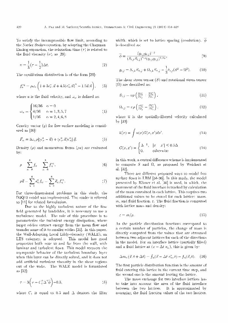
3.1. 2D Submerged landslide (Heinrich [1])The work was done in a ume of 20 m long and0:5 m wide. A triangular rigid wedge with a density of2036:4 kg/m3 and a cross section area equal to 0:125 m2

was allowed to slide freely on an inclined frictionlessshoreline of 45� to horizontal. Water depth was 1:0 mand the wedge was initially 1:0 cm below the watersurface. Figure 2 demonstrates the initial physicalmodel con�guration. The computational domain wasthe same as the physical model and a resolution (latticedimension) of 0:03 m was used.

Pak and Sarfaraz [10] numerically modeled thiscase using FLOW-3D software. They applied threeturbulence models of standard k � ", RNG k � ",and LES, and reported that LES results were moreaccurate.

In Figure 3, experimental surface wave pro�lesare demonstrated and compared with LBM results.Also, the numerical results of this problem, usingthe Eulerian approach by Pak and Sarfaraz [10], andapplying the LES turbulence model, are included andcompared. The �gure shows that the LBM-based code

Figure 2. Initial con�guration of the experimental work,case 1 (in meters).


Figure 3. Experimental and numerical wave pro�les at di�erent times, case 1.

is successful and capable of tracking wave generation,due to the movement of the solid wedge, and is moreaccurate than the Eulerian results, according to itslower RMSE (Root Mean Square Error) values. Also,LBM proves its accuracy in capturing the con�gurationof highly turbulent ow near the beach.

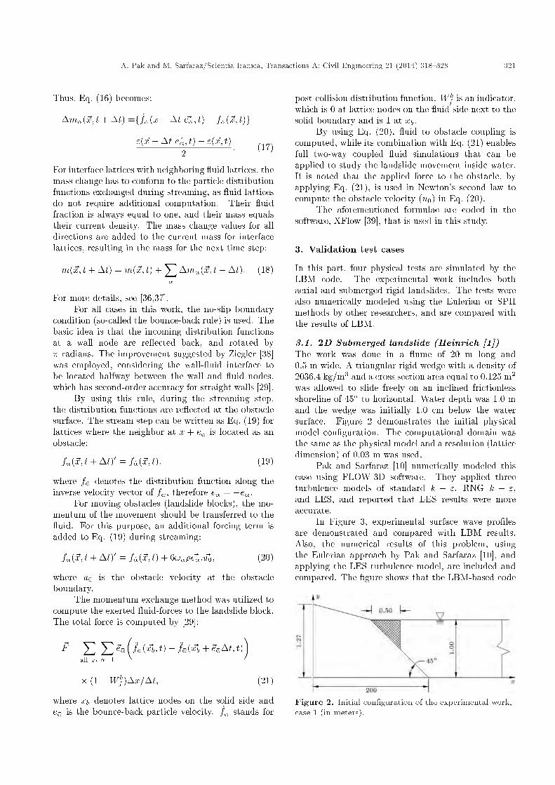
Figure 4 displays and compares experimental andnumerical wave amplitudes at x = 4, 8, 12 m overtime. It is understood that LBM is well capable ofpredicting wave propagation due to the movement ofthe solid wedge in water. RMSE values indicate thatthe LBM-based code is more accurate than the Eulerianapproach for computing the time history of free surfaceelevation due to wave propagation.

As indicated in the introduction section, equa-tions within the Eulerian approach are complex andconsist of high-order derivation terms, whose dis-cretization will generate numerical errors. LBM canovercome these issues, as it contains a simple formu-lation and is straightforward in coupling the ow �eldwith moving obstacles. Furthermore, LBM does notsu�er from numerical issues such as instability. So,in this validation case, LBM provides more accurateresults than the Eulerian technique.

In Figure 5, the velocity �eld and assigned vectorsare presented at di�erent times, showing the stabilityof the model in simulating the problem after the timeat which the wedge has reached the bottom. As thewave propagates towards the right, a clockwise vortexis generated above the wedge, which resists comingdown the run-up water. Also, the maximum velocitymagnitude of these vortexes decreases over time.

3.2. 2D Partially submerged landslide (Yim etal. [23])

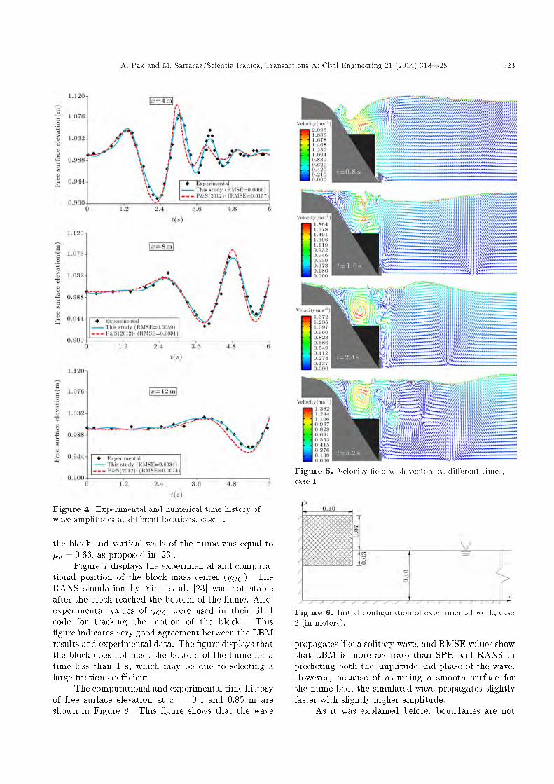
In this section, a solitary wave generated by the verticalfalling of a partially submerged block into water (so-called Scott Russell's wave generator) is considered,and was carried out both physically and numerically(RANS and SPH) by Yim et al. [23]. The experi-ment was performed in a 12 m long ume, with arectangular rigid block weighted 13:3 kg per width,having dimensions of 0:1 m. The ume contained0:1 m depth of water and the bottom of the block wasinitially 3 cm below the still water level (Figure 6). Thecomputational domain was the same as the physicalmodel and a resolution of 4 mm was selected forlattices. The dynamic coe�cient of friction between


Figure 4. Experimental and numerical time history ofwave amplitudes at di�erent locations, case 1.

the block and vertical walls of the ume was equal to�d = 0:66, as proposed in [23].

Figure 7 displays the experimental and computa-tional position of the block mass center (yCG). TheRANS simulation by Yim et al. [23] was not stableafter the block reached the bottom of the ume. Also,experimental values of yCG were used in their SPHcode for tracking the motion of the block. This�gure indicates very good agreement between the LBMresults and experimental data. The �gure displays thatthe block does not meet the bottom of the ume for atime less than 1 s, which may be due to selecting alarge friction coe�cient.

The computational and experimental time historyof free surface elevation at x = 0:4 and 0:85 m areshown in Figure 8. This �gure shows that the wave

Figure 5. Velocity �eld with vectors at di�erent times,case 1.

Figure 6. Initial con�guration of experimental work, case2 (in meters).

propagates like a solitary wave, and RMSE values showthat LBM is more accurate than SPH and RANS inpredicting both the amplitude and phase of the wave.However, because of assuming a smooth surface forthe ume bed, the simulated wave propagates slightlyfaster with slightly higher amplitude.

As it was explained before, boundaries are not


Figure 7. Experimental and computational time historyof mass center position of block, case 2.

Figure 8. Experimental and computational time historyof free surface elevation, case 2.

usually modeled well in SPH. Also, in common SPHcodes, ow incompressibility cannot be guaranteed.Selecting an appropriate smoothing kernel is essentialfor the accuracy and stability of this method and isnot unique for all landslide problems. Unlike theSPH method, boundaries are modeled in a logical wayin LBM. Moreover, it does not need user-dependentparameters, e.g. smoothing kernel functions, and,therefore, LBM provides more accurate results incomparison with SPH.

The location of the falling block, with the velocity


�eld and vectors, are presented in Figure 9 for di�erenttimes. While the block is falling, a counterclockwisevortex develops near the right face of the block andis advected downstream with a slower speed than thephase speed of the generated wave. When the blockreaches the bottom, the velocity magnitude tends todecrease and some small vortexes appear, caused byinteraction between the propagated wave and run-upwater near the block.

3.3. 2D Aerial landslide (Yim et al. [23])The same materials and method as in the previous caseare used in this case, except that the block was kept3 cm initially above the still water with a depth of0:18 m in the ume. Figure 10 shows the experimentaland computed mass center position of the block, whichexhibits good agreement between LBM results andexperimental data. Before the block meets water, nofriction was assumed in the code; hence, it compensatesthe large �d selected in the previous case.

The amplitudes and phase of the generated waveare well computed by LBM at x = 0:4 and 0:85 m


Figure 10. Experimental and computational time historyof mass center position of block, case 3.


(see Figure 11). It is worth noting that since thestill water depth is more than in the previous case,bed friction has less e�ect on the propagated wave;the phase di�erence between LBM and experimentaldata is negligible. There exists noticeable disagreementbetween the experimental and computed results byRANS and SPH after t = 1:5 s.

Figure 12 depicts the block location at di�erenttimes, together with the velocity �eld and vectors. Inview of the fact that the still water depth is more thanthe block height, water overtops the block, and thenre ects back towards the ume. Since the block accel-


erates before going through the water, ow separationis observed near the right end of the block at t = 0:2 s.Similar to the previous case, a counterclockwise vortexappears and is advected with wave propagation, but ismore stretched along the ume direction.

3.4. 3D Submerged landslide (Ataie andNaja� [6])

This part discusses the applicability and e�ciency ofthe LBM method for modeling 3D landslide problems.A rigid rectangular block, with a weight of 14:82 kg,0:3 m in length, 0:2 m in width and 0:13 m in height,was submerged initially on a 30� sloping beach with


a 0:5 m depth of still water (see Figure 13). Allsurfaces were lubricated to eliminate friction and thetest was repeated two times. The ume width was2:5 m; therefore, it simulates a 3D landslide, as happensin the real world. In this experimental work, waterelevation towards the centerline of the ume (along thex axis) was measured at di�erent positions [6].

The computational domain was the same as thephysical model, and a resolution of 8 mm was selected.Mansour-Rezaei and Ataie [20] simulated the sameproblem using SPH in the 3D space using di�erentkernel functions. Experimental and computationalvalues of free surface elevation at x = 1:13 and 2:03 mare shown in Figure 14. It is proved that LBM success-

Figure 13. Initial con�guration of experimental work,case 4 (in meters).


fully overcomes the problems encountered to model thepropagated wave in both amplitude and speed.

The predicted wave by LBM has slightly morespeed, which may be due to existing friction betweenthe block and surface of the beach. The amplitude ofthe �rst trailing is a little under-predicted, which ispossibly caused by using a coarse resolution of lattices.The �gure points out that the calculated wave by SPHhas a considerable phase lag and smaller amplitudes,exhibiting a dissipative manner.

Velocity �elds with vectors along the x-axis atdi�erent times are shown in Figure 15. While theblock slides down, water overtops and pushes the blockto the right side. Also a counterclockwise vortex isobserved on top of the block, which moves upwardsand dissipates during the course of sliding.

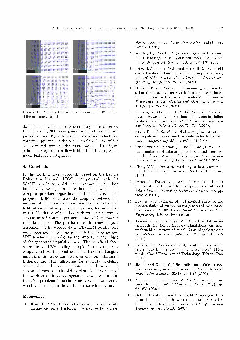
Figure 16 presents the velocity �eld and vectorsover a plane cutting the y-axis at y = 0:43 m. Half the

Figure 15. Velocity �eld with vectors along x-axis atdi�erent times, case 4.


Figure 16. Velocity �eld with vectors at y = 0:43 m fordi�erent times, case 4.

domain is shown due to its symmetry. It is observedthat a strong 3D wave generation and propagationpattern exists. By sliding the block, counterclockwisevortexes appear near the top side of the block, whichare advected towards the ume walls. The �gureexhibits a very complex ow �eld in the 3D case, whichneeds further investigations.

4. Conclusion

In this work, a novel approach, based on the LatticeBoltzmann Method (LBM), incorporated with theWALE turbulence model, was introduced to simulateimpulsive waves generated by landslides, which is acomplex problem regarding the free surface. Theproposed LBM code takes the coupling between themotion of the landslide and variation of the ow�eld into account to predict the propagated impulsivewaves. Validation of the LBM code was carried out bysimulating a 2D submerged aerial, and a 3D submergedrigid landslide. The predicted results showed goodagreement with recorded data. The LBM results weremore accurate, in comparison with the Eulerian andSPH schemes, in predicting the amplitude and phaseof the generated impulsive wave. The bene�cial char-acteristics of LBM coding (simple formulation, easycoupling interaction, and stable and non-challengingnumerical discretization) can overcome and eliminateEulerian and SPH di�culties for accurate modelingof complex and non-linear interaction between thegenerated wave and the sliding obstacle. Extension ofthis work would be advantageous to wave-structure in-teraction problems in o�shore and coastal frameworkswhich is currently in the authors' research program.

References

1. Heinrich, P. \Nonlinear water waves generated by sub-marine and aerial landslides", Journal of Waterways,

Ports, Coastal and Ocean Engineering, 118(3), pp.249-266 (1992).

2. Walder, J.S., Watts, P., Sorensen, O.E. and Janssen,K. \Tsunami generated by subaerial mass ows", Jour-nal of Geophysical Research, 28, pp. 397-400 (2001).

3. Fritz, H.M., Hager, W.H. and Minor H.E. \Near �eldcharacteristics of landslide generated impulse waves",Journal of Waterways, Ports, Coastal and Ocean En-gineering, 130(6), pp. 287-302 (2004).

4. Grilli, S.T. and Watts, P. \Tsunami generation bysubmarine mass failure; Part I: Modeling, experimen-tal validation and sensitivity analysis", Journal ofWaterways, Ports, Coastal and Ocean Engineering,131(6), pp. 283-297 (2005).

5. Panizzo, A., Girolamo, P.D., Di Risio, M., Maistria,A. and Petaccia, A. \Great landslide events in Italianarti�cial reservoirs", Journal of Natural Hazards andEarth System Sciences, 5, pp. 733-740 (2005).

6. Ataie, B. and Naja�, A. \Laboratory investigationson impulsive waves caused by underwater landslide",Coastal Engineering, 55, pp. 989-1004 (2008).

7. Rzadkiewicz, S., Mariotti, C. and Heinrich, P. \Numer-ical simulation of submarine landslides and their hy-draulic e�ects", Journal of Waterways, Ports, Coastaland Ocean Engineering, 123(4), pp. 149-157 (1997).

8. Titov, V.V. \Numerical modeling of long wave run-up", Ph.D. Thesis, University of Southern California,(1997).

9. Imran, J., Parker, G., Lacat, J. and Lee, H. \1Dnumerical model of muddy sub-aqueous and subaerialdebris ows", Journal of Hydraulic Engineering, pp.959-968 (2001).

10. Pak, A. and Sarfaraz, M. \Numerical study of thecharacteristics of surface waves generated by subma-rine landslides", 9th International Congress on CivilEngineering, Isfahan, Iran (2012).

11. Janssen, C. and Krafczyk, M. \A Lattice Boltzmannapproach for free-surface- ow simulations on non-uniform block-structured grids", Journal of Computersand Mathematics with Applications, 59, pp. 2215-2235(2010).

12. Sarfaraz, M. \Numerical analysis of concrete armorlayers' stability in rubble-mound breakwaters", M.Sc.thesis, Sharif University of Technology, Tehran, Iran(2012).

13. Jie, T. and Xubo, Y. \Physically-based uid anima-tion: a survey", Journal of Science in China Series F:Information Sciences, 52(1), pp. 1-17 (2009).

14. Monaghan, J.J. and Kos, A. \Scott Russell's wavegenerator", Journal of Physics of Fluids, 12(3), pp.622-630 (2000).

15. Gotoh, H., Sakai, T. and Hayashi, M. \Lagrangian two-phase ow model for the wave generation process dueto large-scale landslides", Asian and Paci�c CoastalEngineering, pp. 176-185 (2001).


16. Lo, E.Y.M. and Shao, S. \Simulation of near-shoresolitary wave mechanics by an incompressible SPHmethod", Journal of Applied Ocean Research, 24, pp.275-286 (2002).

17. Shao, S.D. and Lo, E.Y.M. \Incompressible SPHmethod for simulating Newtonian and non-Newtonian ows with a free surface", Journal of Advances inWater Resources, 26(7), pp. 787-800 (2003).

18. Shao, S.D. and Gotho, H. \Turbulence particle modelsfor tracking free surfaces", Journal of Hydraulic Re-search, 43(3), pp. 276-289 (2005).

19. Ataie, B. and Shobeyri, G. \Numerical simulation oflandslide impulsive waves by incompressible smoothedparticle hydrodynamics", International Journal of Nu-merical Methods in Fluids, 56, pp. 209-232 (2008).

20. Mansour-Rezaei, S. and Ataie, B. \Compressiblesmoothed particle hydrodynamics for numerical simu-lation of impulsive waves", (in Farsi), Iranian Journalof Hydraulics, 4(1), pp. 63-73 (2009).

21. M�uller, M., Charypar, D. and Gross, M. \Particle-based uid simulation for interactive applications",Proceeding of the ACM SIGGRAPH/EurographicsSymposium on Computer Animation, Switzerland, pp.154-159 (2003).

22. Crespo, A.J.C. \Application of the smoothed particlehydrodynamics model SPHysics to free-surface hydro-dynamics", Ph.D. Thesis, University of De Vigo, Italy(2008).

23. Yim., S.C., Yuk, D., Panizzo, A., Di Risio, M. andLiu, P.L.F. \Numerical simulation of wave generationby a vertical plunger using RANS and SPH models",Journal of Waterways, Ports, Coastal, and OceanEngineering, 134(3), pp. 1-17 (2008).

24. Ghassemi, A. and Pak, A. \Numerical study of factorsin uencing relative permeabilities of two immiscible uids owing through porous media using latticeBoltzmann method", Journal of Petroleum Scienceand Engineering, 72, pp. 135-145 (2013).

25. Chen, C. and Doolen, G.D. \Lattice Boltzmannmethod for uid ows", Journal of Annual Review ofFluid Mechanics, 30, pp. 329-364 (1998).

26. Strumolo, G. and Viswanathan, B. \New directions incomputational aerodynamics", Journal of Physics andWorld, 10, pp. 45-49 (1997).

27. Liao, Q. and Jen, T.C. \Application of lattice Boltz-mann method in uid ow and heat transfer", Com-putational Fluid Dynamics Technologies and Appli-cations, Edited by Minin, I.V. and Minin, O.V.,Published by Intech, pp. 29-68 (2011).

28. Succi, S., The lattice Boltzmann Equation for FluidDynamics and Beyond, Clarendon Press, Oxford(2001).

29. Dazhi, Y., Mei, R., Luo, L.S. and Shyy, W. \Viscous ow computations with the method of lattice Boltz-mann equation", Journal of Progress in AerospaceSciences, 39, pp. 329-367 (2003).

30. Lou, L.S. \Theory of the lattice Boltzmann method:Lattice Boltzmann models for non-ideal gases", Jour-nal of Physical Review, E62, pp. 4982-4996 (2000).

31. Garnier, E., Adams, N. and Sagaut, P., Large EddySimulation for Compressible Flows, Springer (2009).

32. Weickert, M., Teike, G., Schmidt, O. and Sommerfeld,M. \Investigation of the LES WALE turbulence modelwithin the lattice Boltzmann framework", Journal ofComputes and Mathematics with Applications, 59, pp.2200-2214 (2010).

33. Hou, S., Sterling, J., Chen, S. and Doolen, G.D. \Alattice Boltzmann subgrid model for high Reynoldsnumber ows", Fields Institute Communications, 6,pp. 151-165 (1996).

34. Gunstensen, A.K., Rothman, D.H., Zaleski, S. andZanetti, G. \Lattice Boltzmann model of immiscible uids", Journal of Physical Review, 43(8), pp. 4320-4327 (1991).

35. Ginzburg, I. and Steiner, K. \A free-surface lat-tice Boltzmann method for modelling the �lling ofexpanding cavities by Bingham uids", Journal ofPhilosophical Transactions: Mathematical, Physicaland Engineering Sciences, 360, pp. 453-466 (2002).

36. K�orner, C., Thies, M., Hofmann, T., Th�urey, N. andR�ude, U. \Lattice Boltzmann model for free surface ow for modeling foaming", Journal of StatisticalPhysics, 121, pp. 179-196 (2005).

37. Th�urey, N. \Physically based animation of free surface ows with the lattice Boltzmann method", Ph.D.Thesis, University of Erlangen-N�urnberg, Bavaira,Germany (2007).

38. Ziegler, D.P. \Boundary conditions for lattice Boltz-mann simulations", Journal of Statistical Physics, 71,pp. 1171-1177 (1993).

39. Next Limit Inc. \XFlow user's manual", Madrid, Spain(2012).

Biographies

Ali Pak is Professor of Civil Engineering at SharifUniversity of Technology, Tehran, Iran. He has exten-sive publications in various �elds of engineering, suchas numerical modeling of soil structures, petroleumgeomechanics, environmental geotechnics, liquefactionmodeling, and hydraulic fracturing.

Mohammad Sarfaraz obtained a BS degree in CivilEngineering from the Power and Water Universityof Technology, Iran, in 2010, and an MS degree inGeotechnical Engineering from Sharif University ofTechnology, Tehran, Iran, in 2012. He ranked �rstamong all students both in BS and MS programs.His main research interests include: wave-structureinteraction, coastal and o�shore structures, geotechni-cal earthquake engineering, lattice Boltzmann Method,and impulsive water waves generated by landslides.

lattice boltzmann method for simulating impulsive water

Documents