lattice dynamics studies of negative thermal expansion due
TRANSCRIPT

University of ConnecticutOpenCommons@UConn
Doctoral Dissertations University of Connecticut Graduate School
11-27-2018
Lattice Dynamics Studies of Negative ThermalExpansion Due to Two Low-temperature LatticeInstabilities.SAHAN UDDIKA HANDUNKANDAUniversity of Connecticut - Storrs, [email protected]
Follow this and additional works at: https://opencommons.uconn.edu/dissertations
Recommended CitationHANDUNKANDA, SAHAN UDDIKA, "Lattice Dynamics Studies of Negative Thermal Expansion Due to Two Low-temperatureLattice Instabilities." (2018). Doctoral Dissertations. 2021.https://opencommons.uconn.edu/dissertations/2021
Lattice Dynamics Studies of NegativeThermal Expansion Due to Two
Low-temperature Lattice Instabilities
Sahan Handunkanda, Ph.D.University of Connecticut, 2018
ABSTRACT
Here I present a complete study of lattice dynamics of negative thermal ex-
pansion (NTE) material Scandium trifluoride (ScF3) and discovery of NTE in
mercurous iodide (Hg2I2). An inelastic x-ray scattering (IXS) study of ScF3
reveals copious evidence of an incipient soft-mode instability indicating that
the T=0 state of ScF3 is very close to a structural quantum phase transition
(SQPT). Is the anomalously strong and thermally persistent NTE behavior of
ScF3 a consequence of the SQPT? In order to address that, we have explored
the coefficient of thermal expansion (CTE) and soft mode behavior of a sec-
ond stoichiometric compound, situated near a SQPT. A detailed side-by-side
comparison of the metal trifluorides and mercurous halides suggest strong
similarities and a generic connection between the fluctuating ground state
of incipient ferroelastic materials and SNTE. We find experimental evidences

Sahan Handunkanda - University of Connecticut - 2018
for two- dimensional nanoscale correlations exist at momentum-space regions
associated with possibly rigid rotations of the perovskite octahedra of ScF3.
The discussion is extended by addressing the extent to which rigid octahedral
motion describes the dynamical fluctuations behind NTE by generalizing a
simple model supporting a single floppy mode that is often used to heuris-
tically describe instances of NTE. Temperature-dependent infrared reflection
measurement on single crystal ScF3 is performed to understand the zone cen-
ter lattice dynamics of ScF3. In addition, I also carried out an instrumentation
development project in the laboratory at the Department of Physics which will
be briefly discussed in the last chapter.

Lattice Dynamics Studies of NegativeThermal Expansion Due to Two
Low-temperature Lattice Instabilities
Sahan Handunkanda
M.S. Physics, University of Connecticut, Storrs, CT, 2014B.S. Physics, University of Colombo, Sri Lanka, 2009
A DissertationSubmitted in Partial Fulfillment of the
Requirements for the Degree ofDoctor of Philosophy
at theUniversity of Connecticut
2018

Copyright by
Sahan Handunkanda
2018
ii

APPROVAL PAGE
Doctor of Philosophy Dissertation
Lattice Dynamics Studies of NegativeThermal Expansion Due to Two
Low-temperature Lattice Instabilities
Presented bySahan Handunkanda, M.S. Physics, B.S. Physics
Major AdvisorJason Hancock
Associate AdvisorBarrett Wells
Associate AdvisorDouglas Hamilton
University of Connecticut2018
iii

ACKNOWLEDGEMENTS
This thesis would not have been possible without collective effort and co-operation of many people. First of all, I would like to express my deepestappreciation to my PhD advisor Dr. Jason Hancock. I am greatly thankful forthe faith that my advisor had on me from the day we first met, especially bywelcoming me as his first graduate student. Throughout my PhD, I enjoyedand learnt from his knowledge and expertise in condensed matter research.He has given enormous encouragement and assistance while being patiencewith me over the past six and half years, something I truly appreciate. Hischaracteristic traits eventually helped me to develop as a skilled physicist.
I also offer my sincere gratitude to Dr. Barrett Wells and Dr. Douglas Hamiltonwho served me as associate advisors. Apart from Dr. Wells’s proficiency andvaluable discussion on my research I am also thankful to Dr. Wells for recom-mending me to talk with at the time new faculty member, Dr. Hancock aboutprospective research opportunities. I would like to thank Dr. Hamilton forhis advise and encouraging words on writing which is the key to a successfulscientific career.
I would like to express my gratitude to the beamline scientist Dr. AymanSaid at sector 30, Advanced Photon Source, Argonne National Laboratory forsupporting us while we were taking our data on Scandium trifluoride samples.He provided a great amount of technical support during multiple beamtimes,which I never forget and greatly appreciate.
Successful experimentation is never possible without having quality samples.My special thanks goes to Dr. Vladimir Voronov in Kirensky Institute of Physicsin Russia for proving us isotopically pure, single-crystalline Scandium triflu-oride samples and Dr. Sudhir Trivedi in Brimrose Technology Corporation,Sparks, Maryland for proving us single crystalline Mercurous Halide samples.
Theoretical collaborates are a vital part of a research study. The discussionwe had and their insight on interpreting the experimentation results helped usto communicate and efficiently present the research findings and I would takethis opportunity to thank the team led by Dr. Peter Littlewood then director ofArgonne National Laboratory, Dr. Gian Guzman-Verri, and Dr.Richard Brier-ley in Yale University.
My sincere thanks goes to Dr. Joseph Budnick, Dr. William Hines, Dr. Boris
iv

Sinkovic, Dr. Gerald Dunne and Dr. Gayanath Fernando for the valuable con-versations that we had on our experimentation results. I appreciate Dr. IlyaSochnikov and Dr. Diego Valente for accepting the invitation to take a part inmy dissertation committee on such short notice. I would also like to thank toDr. Dave Perry, someone who is always willing to help, especially when I needto figure out mechanical part necessary for my research work. Special thanksgoes to Alan Chasse, the machine shop engineer for making all the necessarymechanical parts used in instrumentation development. I would also like tothank the former office staff Dawn, Kim and Babara as well as the current officestaff in Physics, Micki, Anna, Caroline and Alessandra for their support inadministrative works.
I would like to thank all my group members Erin Curry, Donal Sheets andConnor Occhialini whom I had a great time working with and had a lot of funduring my PhD in and out of the laboratory. The support and encouragementprovided by Sri Lankan community at UConn, my batch mates Niraj, Zhiwei,Udaya, Susini, Katya and Dale at the difficult time during my stay at Storrs arehugely appreciated.
Last but not least I thank my dear parents, sister and my beloved wife Awanthifor their endless support and love provided me during the past few years.
v

TABLE OF CONTENTS
Ch. 1 : Introduction . . . . . . . . . . . . . . . . . . . . . . . . . . . . . . . . . . . . . . . . . . . . . . . . . 11.1. Thermal expansion . . . . . . . . . . . . . . . . . . . . . . . . . . . . . . . . . . . . . . . . . . . . . 11.2. Lattice Dynamics . . . . . . . . . . . . . . . . . . . . . . . . . . . . . . . . . . . . . . . . . . . . . . . 21.3. Negative thermal expansion . . . . . . . . . . . . . . . . . . . . . . . . . . . . . . . . . . . . . 91.3.1. Negative thermal expansion from phase competition . . . . . . . . . . . . . 101.3.2. Negative thermal expansion from framework dynamics . . . . . . . . . . 131.4. Theoretical consideration of negative thermal expansion . . . . . . . . . . . 161.4.1. Grneisen theory and thermal expansion . . . . . . . . . . . . . . . . . . . . . . . . . 161.4.2. Rigid unit mode picture . . . . . . . . . . . . . . . . . . . . . . . . . . . . . . . . . . . . . . . 171.4.3. Tension effect and NTE . . . . . . . . . . . . . . . . . . . . . . . . . . . . . . . . . . . . . . . . 211.4.4. Thermodynamics of NTE materials . . . . . . . . . . . . . . . . . . . . . . . . . . . . . 211.5. Perovskites . . . . . . . . . . . . . . . . . . . . . . . . . . . . . . . . . . . . . . . . . . . . . . . . . . . . 221.6. Trifluorides and their structures . . . . . . . . . . . . . . . . . . . . . . . . . . . . . . . . . . 231.7. Scandium trifluoride(ScF3) . . . . . . . . . . . . . . . . . . . . . . . . . . . . . . . . . . . . . . 251.7.1. Negative thermal expansion in ScF3 . . . . . . . . . . . . . . . . . . . . . . . . . . . . 251.7.2. Pressure induced phase transition in ScF3 . . . . . . . . . . . . . . . . . . . . . . . 261.7.3. Electronic structure of ScF3 . . . . . . . . . . . . . . . . . . . . . . . . . . . . . . . . . . . . 271.8. Motivation . . . . . . . . . . . . . . . . . . . . . . . . . . . . . . . . . . . . . . . . . . . . . . . . . . . . . 29
Ch. 2 : Lattice dynamics study of ScF3 using inelastic x-ray scattering . . . 312.1. Introduction to Inelastic X-ray Scattering . . . . . . . . . . . . . . . . . . . . . . . . . . 312.1.1. IXS advantages over other spectroscopic techniques . . . . . . . . . . . . . . 322.2. Scattering theory . . . . . . . . . . . . . . . . . . . . . . . . . . . . . . . . . . . . . . . . . . . . . . . 342.2.1. Dynamic structure factor (S(
−→Q, ω)) . . . . . . . . . . . . . . . . . . . . . . . . . . . . . 39
2.2.2. Quantum mechanical perspective . . . . . . . . . . . . . . . . . . . . . . . . . . . . . . 412.2.3. Scattering cross section . . . . . . . . . . . . . . . . . . . . . . . . . . . . . . . . . . . . . . . . 482.2.4. IXS for phonons . . . . . . . . . . . . . . . . . . . . . . . . . . . . . . . . . . . . . . . . . . . . . . 492.2.5. Scattering from phonons in theoretical perspective . . . . . . . . . . . . . . 512.3. Inelastic X-ray Scattering on ScF3 . . . . . . . . . . . . . . . . . . . . . . . . . . . . . . . . . 552.3.1. The Experiment . . . . . . . . . . . . . . . . . . . . . . . . . . . . . . . . . . . . . . . . . . . . . . 562.3.2. Single crystal ScF3 . . . . . . . . . . . . . . . . . . . . . . . . . . . . . . . . . . . . . . . . . . . . 562.3.3. Lattice parameter measurement . . . . . . . . . . . . . . . . . . . . . . . . . . . . . . . . 612.3.4. Phonon dispersion relation . . . . . . . . . . . . . . . . . . . . . . . . . . . . . . . . . . . . 622.3.5. M-R branch and NTE . . . . . . . . . . . . . . . . . . . . . . . . . . . . . . . . . . . . . . . . . 632.3.6. M-R branch and phase transition . . . . . . . . . . . . . . . . . . . . . . . . . . . . . . . 642.3.7. Central peak of ScF3 . . . . . . . . . . . . . . . . . . . . . . . . . . . . . . . . . . . . . . . . . . 672.3.8. What causes central peak? . . . . . . . . . . . . . . . . . . . . . . . . . . . . . . . . . . . . . 682.3.9. Central peak of ScF3 and mode softening . . . . . . . . . . . . . . . . . . . . . . . . 72
vi

2.3.10. Quantum phase transition in ScF3 and phase transitions in othertransition metal trifluorides . . . . . . . . . . . . . . . . . . . . . . . . . . . . 76
2.3.11. ScF3 systems and disorder . . . . . . . . . . . . . . . . . . . . . . . . . . . . . . . . . . . . . 782.3.12. Transverse motion of F atoms . . . . . . . . . . . . . . . . . . . . . . . . . . . . . . . . . . 812.3.13. Elastic parameters of ScF3 . . . . . . . . . . . . . . . . . . . . . . . . . . . . . . . . . . . . . 822.3.14. Modeling IXS data using Damped Harmonic Oscillator(DHO) . . . . 86
Ch. 3 : Comparative study of two incipient ferroelastics, ScF3 and Hg2I2 923.1. Introduction . . . . . . . . . . . . . . . . . . . . . . . . . . . . . . . . . . . . . . . . . . . . . . . . . . . 923.2. Low-T structure and scattering evidence for the IFE behavior of
Hg2I2 and ScF3 . . . . . . . . . . . . . . . . . . . . . . . . . . . . . . . . . . . . . . . . . . . . . . 943.3. Discussion and SNTE material design principles . . . . . . . . . . . . . . . . . . . 98
Ch. 4 : Thermal Diffuse Scattering on ScF3 . . . . . . . . . . . . . . . . . . . . . . . . . . . 1064.1. Introduction to diffuse scattering . . . . . . . . . . . . . . . . . . . . . . . . . . . . . . . . . 1064.2. Diffuse Scattering study of single-crystalline compound ScF3 . . . . . . . 1074.2.1. Experiment . . . . . . . . . . . . . . . . . . . . . . . . . . . . . . . . . . . . . . . . . . . . . . . . . . 1074.2.2. Negative thermal expansion of ScF3 and diffuce scattering . . . . . . . 1084.2.3. Results and discussion . . . . . . . . . . . . . . . . . . . . . . . . . . . . . . . . . . . . . . . . 110
Ch. 5 : Two dimensional constrained lattice model to study ScF3 lattice . 1145.1. Introduction . . . . . . . . . . . . . . . . . . . . . . . . . . . . . . . . . . . . . . . . . . . . . . . . . . . 1145.2. Two-dimensional constrained lattice model . . . . . . . . . . . . . . . . . . . . . . . 1155.3. Application of model to experimental results . . . . . . . . . . . . . . . . . . . . . . 121
Ch. 6 : Infrared study of ScF3 . . . . . . . . . . . . . . . . . . . . . . . . . . . . . . . . . . . . . . . . 1256.1. Introduction . . . . . . . . . . . . . . . . . . . . . . . . . . . . . . . . . . . . . . . . . . . . . . . . . . . 1256.2. Measurements . . . . . . . . . . . . . . . . . . . . . . . . . . . . . . . . . . . . . . . . . . . . . . . . . 1266.3. Lorentzian model fitting . . . . . . . . . . . . . . . . . . . . . . . . . . . . . . . . . . . . . . . . 1276.4. Factorized model fitting . . . . . . . . . . . . . . . . . . . . . . . . . . . . . . . . . . . . . . . . . 1286.5. Zone center modes . . . . . . . . . . . . . . . . . . . . . . . . . . . . . . . . . . . . . . . . . . . . . 1326.6. Infrared measurement results . . . . . . . . . . . . . . . . . . . . . . . . . . . . . . . . . . . 1346.6.1. Discussion . . . . . . . . . . . . . . . . . . . . . . . . . . . . . . . . . . . . . . . . . . . . . . . . . . . 137
Ch. 7 : Resonant Ultrasound Spectroscopy . . . . . . . . . . . . . . . . . . . . . . . . . . . . 1477.1. Introduction . . . . . . . . . . . . . . . . . . . . . . . . . . . . . . . . . . . . . . . . . . . . . . . . . . . 1477.2. Elastic properties and constitute equations . . . . . . . . . . . . . . . . . . . . . . . . 1487.2.1. Symmetries in cubic systems and other important properties . . . . . . 1517.3. Resonant ultrasound spectroscopy fundamentals . . . . . . . . . . . . . . . . . . 1547.4. ScF3 sample and RUS setup used . . . . . . . . . . . . . . . . . . . . . . . . . . . . . . . . . 1567.5. RUS measurement on ScF3 . . . . . . . . . . . . . . . . . . . . . . . . . . . . . . . . . . . . . . 158
Ch. 8 : Instrumentation Development . . . . . . . . . . . . . . . . . . . . . . . . . . . . . . . . 1648.1. Introduction . . . . . . . . . . . . . . . . . . . . . . . . . . . . . . . . . . . . . . . . . . . . . . . . . . . 164
vii

8.2. Fourier Transformed Infrared Spectrometer . . . . . . . . . . . . . . . . . . . . . . . 1668.2.1. Mirror design . . . . . . . . . . . . . . . . . . . . . . . . . . . . . . . . . . . . . . . . . . . . . . . . 1678.2.2. Vibration-free, cryogen-free optical cryocooler . . . . . . . . . . . . . . . . . . . 1728.3. Time-Domain Terahertz(TD- THz) spectrometer . . . . . . . . . . . . . . . . . . . 1738.3.1. Introductory to TD-THz spectrometer . . . . . . . . . . . . . . . . . . . . . . . . . . 1758.3.2. Our TD-THz spectrometer . . . . . . . . . . . . . . . . . . . . . . . . . . . . . . . . . . . . . 1788.3.3. THz signal . . . . . . . . . . . . . . . . . . . . . . . . . . . . . . . . . . . . . . . . . . . . . . . . . . . 185
App. A : Construction of an optical system . . . . . . . . . . . . . . . . . . . . . . . . . . . 186
Bibliography . . . . . . . . . . . . . . . . . . . . . . . . . . . . . . . . . . . . . . . . . . . . . . . . . . . . . . .
viii

LIST OF FIGURES
1.1.1 (a) The anharmonic potential is shown. The potential is asym-metric, so that increases in temperature (i.e. the amplitude ofoscillation of atoms) leads to an increase in the mean interatomicseparation, and hence to thermal expansion. (b) The harmonicpotential is symmetric and as the temperature is increased themean separation remains the same hence no thermal expansion . 3
1.2.1 A linear chain of identical atoms. . . . . . . . . . . . . . . . . . . . . . . . . . . . . . . . 41.2.2 Dispersion relation of the 1D chain of atoms. . . . . . . . . . . . . . . . . . . . . 61.2.3 A linear chain of two atomic species . . . . . . . . . . . . . . . . . . . . . . . . . . . . 71.2.4 Dispersion relation of the 1D chain of two different atoms. . . . . . . . . 91.3.1 NTE in ferroelectrics. (a) Unit cell volume of 0.5PbTiO3-0.5(Bi1−xLax)FeO3
(x = 0.0, 0.1, and 0.2) as function of temperature. FE and PE meanferroelectric and paraelectric, respectively. Taken from [1]. (b)Thermal expansion coefficient of volume in PbTiO3.Taken from[2]. . . . . . . . . . . . . . . . . . . . . . . . . . . . . . . . . . . . . . . . . . . . . . . . . . . . . . . . . 11
1.3.2 NTE due to valance transitions. (a)Temperature dependence ofthe unit cell volume of BiNiO3. Low pressure-temperature andhigh pressure-temperature data are drawn as open and closedcircles, and crosses show the weighted average volume in thetransition region. From [3]. (b)The dilatometric linear thermalexpansion of Bi0.95La0.05NiO3 on heating and cooling showing a20 K hysteresis. From [3]. (c)Temperature evolution of structureparameter unit cell volume of Sm2.75C60.From[4] . . . . . . . . . . . . . . . 12
1.3.3 NTE in magnetic materials. (a) Temperature dependence of theunit-cell volume of MnF3 . The Neel temperature, TN is shown.From [5]. (b) Relative length changes ∆L/L0 of ferromagnetGdAgMg for various magnetic fields. From [6] . . . . . . . . . . . . . . . . 14
1.3.4 Negative thermal expansion in ZWO. Filled circles represent neu-tron diffraction data while open circle represent dilatometrydata. Taken from [7]. . . . . . . . . . . . . . . . . . . . . . . . . . . . . . . . . . . . . . . . . 15
1.4.1 Rotation of 2D perovskite leads to an area reduction. . . . . . . . . . . . . . 201.4.2 Representation of the tension effect. A linear linkage of three atoms
is shown in left. This can distort such a way that the central atomdisplaces transverse direction or the two end atoms displace inopposite ways. In both cases the bonds stay in rigid and the twoend atoms move inwards in the vertical direction. Taken from [8] 22
1.6.1 Global structural phase diagram of MF3 type perovskites. . . . . . . . . . 24
ix

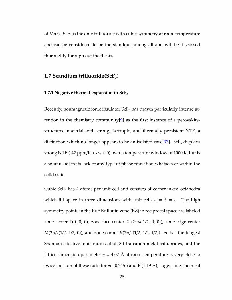
1.7.1 Pressure-temperature phase diagram for ScF3. The dashed line isa guide to the eye. Two layers of octahedra in both the cubicand the rhombohedral ReO3 structures (viewed along [111]) areshown. Upon pressurization, octahedral tilts fold the structureso that it is more compact and reduce the symmetry from cubicto rhombohedral. Taken form [9] . . . . . . . . . . . . . . . . . . . . . . . . . . . . . . 28
2.1.1 Excitations that may probe using IXS, From [10] . . . . . . . . . . . . . . . . . . 31
2.2.1 X-ray scattering from an arbitrary atoms . . . . . . . . . . . . . . . . . . . . . . . . . 34
2.2.2 Radiation from source (S) to detector (D) via the sample . . . . . . . . . . . 37
2.2.3 Reflection geometry where the blue solid circle represents the jth
atom where −→r j and −→r initiate at the unit cell origin . . . . . . . . . . . . . . 38
2.2.4 Typical features appear on high energy resolution inelastic scatter-ing spectrum . . . . . . . . . . . . . . . . . . . . . . . . . . . . . . . . . . . . . . . . . . . . . . . . 50
2.2.5 Phonon creation is shown on left and phonon annihilate processon right . . . . . . . . . . . . . . . . . . . . . . . . . . . . . . . . . . . . . . . . . . . . . . . . . . . . 51
2.3.1 Simple cubic structure of ScF3 lattice where pink spheres are Scatoms and orange spheres represent F atoms. From [11] . . . . . . . . . 57
2.3.2 Schematic of IXS spectrometer layout (a) and photograph (b) of the9 m arm of the spectrometer at sector 30 of APS. The schematicis not to scale. The main components, the direction of incidentbeam and scattered beam are shown. Sample is mounted ona four circle rotational mount and the detector array is kept asmuch as close to the sample. Analyzer array is mounted at farend of the arm which is capable of rotate about 32 degrees whichis corresponding to maximum of 75 nm−1 momentum transfer. . . . 57
2.3.3 (a) Single crystal ScF3 received from Vladimir Voronov. We namedthem for identification purpose in future usage. (b) Simple cubicstructure formation of ScF3 lattice drawn in to scale where purplespheres are Sc atoms and red spheres represent F atoms. . . . . . . . . 58
2.3.4 (a) Crystal mount used in sector 30 experiment. (b) Dimensionsof the crystal Gamma. Crystal sits on wax in order to carry outX-ray diffraction measurement. . . . . . . . . . . . . . . . . . . . . . . . . . . . . . . . 59
2.3.5 Diffraction spots appeared on 2D area detector. Crystal plane isz=o and sample Gamma is used. Lattice planes are shown indotted lines . . . . . . . . . . . . . . . . . . . . . . . . . . . . . . . . . . . . . . . . . . . . . . . . . 60
2.3.6 X -ray diffraction data on powder ScF3 sample . . . . . . . . . . . . . . . . . . . 60
x

2.3.7 (a) Mosaic width ∼ 0.0020, as measured on the strong (H,K,L) =(1,1,0) Bragg reflection indexed to the four-atom simple cubiccell (lattice parameter a = 4.016 A at temperature T = 300 K) (b)Lattice volume as a function of temperature determined fromtracking the Bragg peak (3,0,0) in single-crystalline ScF3. Inset:The lattice volume over a larger thermal window determined onpowder samples[9]. . . . . . . . . . . . . . . . . . . . . . . . . . . . . . . . . . . . . . . . . . . 61
2.3.8 Overview of the lattice mode dispersion at select momenta andenergies. Strong branch softening along the M − R cut is shownby arrows. The longitudinal (LA) and transverse (TA) acousticbranches are shown. Black solid lines are a guide to the eye. Redcircles in the inset mark the momenta R + δ (2.39,1.43,0.45) andM + ε (2.39,1.43,0.02) . . . . . . . . . . . . . . . . . . . . . . . . . . . . . . . . . . . . . . . . . 62
2.3.9 〈100〉 planar section of the octahedra, illustrating the displacementpattern of modes attributed to NTE. The area of the box in (b) isreduced by cos2θ of the area in (a) . . . . . . . . . . . . . . . . . . . . . . . . . . . . 64
2.3.10 First Brillouin zone of simple cubic material ScF3. High symmetrypoints are shown as well. . . . . . . . . . . . . . . . . . . . . . . . . . . . . . . . . . . . . . 65
2.3.11 (a) The lowest vibrational modes at the M point.(M+3 distortion) (b)
The lowest vibrational modes at the R point. The rhombohedralphase can be described as a static tilt according to the R+
4 pattern. 662.3.12 (a) Inelastic spectra of SrTiO3 measured at several temperatures.
Left side shows the soft mode behavior and right side showsdivergence of central peak. From [12]. (b) Inelastic spectra ofSrTiO3 (left) and KMnF3 (right) for approximately equal ∆T=T-Tc. From [12]. . . . . . . . . . . . . . . . . . . . . . . . . . . . . . . . . . . . . . . . . . . . . . . . 68
2.3.13 Central peak due to defects and impurities. (a) Integrated centralpeak intensity of hydrogen reduced SrTiO3 as a funtion of T-Tc[13]. (b) The temperature dependence of the central peak heightof the as-grown KH3(SeO3)2 crystal (+) and the crystals usedrepeatedly (0, ,x)[14] . . . . . . . . . . . . . . . . . . . . . . . . . . . . . . . . . . . . . . . . . 70
2.3.14 Broad and narrow features within the central peak. Solid anddotted curves in (a) represent fitting models, Lorenzian squared
and Lorenzian function respectively[15]. (b) X-ray scans of12
(1,1,5) R point along [0 1 1] direction with 100 keV photon energybeam hitting at the center of the crystal and (c) beam hitting thecrystal corner of the crystal. )[16] . . . . . . . . . . . . . . . . . . . . . . . . . . . . . 71
2.3.15 Color maps of the IXS signal at the (a) M (b) R points in reciprocalspace . . . . . . . . . . . . . . . . . . . . . . . . . . . . . . . . . . . . . . . . . . . . . . . . . . . . . . . 73
2.3.16 Color maps of the IXS signal at the (c) M +ε, and (d) R + δ pointsin reciprocal space. . . . . . . . . . . . . . . . . . . . . . . . . . . . . . . . . . . . . . . . . . . 73
xi

2.3.17 Resolution convoluted fitting of the IXS data in figure 2.3.16 resultsin squared mode energies . . . . . . . . . . . . . . . . . . . . . . . . . . . . . . . . . . . . 74
2.3.18 Resolution convoluted fitting of the IXS data in figure 2.3.16 resultsin elastic peak intensity. Elastic peak begins to appear near 80 K,which is 120 K above the extrapolated transition temperature. . . . 75
2.3.19 Central peak intensity observed in SrTiO3 [17]. Elastic peak beginsto appear 25 K above the transition and the intensity reaches it’smaximum at the transition temperature. . . . . . . . . . . . . . . . . . . . . . . . 75
2.3.20 Cubic and rhombahedral unit cells associated with two phasesof transition metal trifluorides other than ScF3 are shown. Asshown the rhombahedral phase is associated with rotated ScF6
sub units. Gray circles represent scandium atoms and light bluecircles represent fluorine atoms. . . . . . . . . . . . . . . . . . . . . . . . . . . . . . . . 77
2.3.21 Structural phase diagram showing the c-r phase boundary vs theB-site mean radius in 3d transition metal trifluorides and in thesolid solutions Sc1xAlxF3 and Sc1xYxF3. Data taken from Refs[18, 19, 20, 21, 22]. . . . . . . . . . . . . . . . . . . . . . . . . . . . . . . . . . . . . . . . . . . . 79
2.3.22 Disorder phase diagram for ScF3. Compositional disorder is quan-tified via the B-site variance σ2
B = 〈 rB - 〈rB〉 〉2, which has the effect
of increasing the stability of the lowersymmetry, rhombohedralstructural phase. Red and orange symbols show the effect of Yand Al substitution, respectively. Dotted lines indicate a linearfit to the Tc(σ2
B), not including the pure sample ScF3. The verti-cal axis intercept reveals a temperature scale ∼ 80-100 K,wherecentral peak elastic scattering and thermal expansion saturationare also observed in pure ScF3 . . . . . . . . . . . . . . . . . . . . . . . . . . . . . . . . 81
2.3.23 Transverse vibrations of Fluorine atom . . . . . . . . . . . . . . . . . . . . . . . . . . 822.3.24 Acoustic phonon energies along different directions in reciprocal
space. The slope simply gives the acoustic velocities of corre-sponding modes along different directions for ScF3. LA andTA stands for longitudinal acoustics and transverse acousticsrespectively . . . . . . . . . . . . . . . . . . . . . . . . . . . . . . . . . . . . . . . . . . . . . . . . . 83
2.3.25 Poisson ratio obtained from elastic parameters . . . . . . . . . . . . . . . . . . . 852.3.26 Youngs modulus obtained using elastic parameters . . . . . . . . . . . . . . . 862.3.27 Representative resolution function collected at 6K from plexiglass
co-mounted with the sample . . . . . . . . . . . . . . . . . . . . . . . . . . . . . . . . . 882.3.28 Schematic of the dynamical structure factor used to fit the data . . . . 892.3.29 Sample of fit quality at momentum points R (left column) and M
(right column). The red points and blue lines resemble data andthe fit respectively. . . . . . . . . . . . . . . . . . . . . . . . . . . . . . . . . . . . . . . . . . . . 90
2.3.30 Sample of fit quality at momentum points R+δ (left column) andM + ε (right column). . . . . . . . . . . . . . . . . . . . . . . . . . . . . . . . . . . . . . . . . 91
xii

3.2.1 Structural phase diagrams of (a) 3d transition metal trifluorides and(b) mercurous halides. Insets show the basic volume-definingpolyhedral units: (a) the BF6 octahedraon and (b) the elongatedsquare dipyramid (ESD). Development of the structure for (c)the trifluorides and (d) the mercurous halides with the ionicradii indicated as spheres. The basic polyhedral structural unitis superposed in each case. (e) Comparison of the observedbond distances (symbols) and expectations based on hard spherepacking (dashed lines). . . . . . . . . . . . . . . . . . . . . . . . . . . . . . . . . . . . . . . 95
3.2.2 Temperature-dependent lattice parameters of (a,c) ScF3, TiF3, and(b,d,f) Hg2I2, and Hg2Br2. (e) shows a schematic free energylandscape of realized and incipient ferroelastics. Arrows showthe fluctuation domain in each case. . . . . . . . . . . . . . . . . . . . . . . . . . . . 96
3.2.3 Rocking curves measured at (330) bragg peak for optical and detec-tor quality Hg2Br2 and Hg2I2 crystals cleaved along 〈110〉 planesgrown by physical vapor deposition method by Brimrose Tech-nology Cooperation. . . . . . . . . . . . . . . . . . . . . . . . . . . . . . . . . . . . . . . . . . 97
3.3.1 Structure of 3d transition metal trifluorides in the (a) high-temperaturecubic phase and (b) the low-temperature rhombohedral phase.Structure of the mercurous halides in (c) the high-temperaturebody-centered tetragonal and (d) low-temperature orthorhom-bic phases. Inelastic X-rays scattering measurement of (e) ScF3
at the simple-cubic R point, corresponding to the soft mode ofthe rhombohedral transition and (f) Hg2I2 at the BCT X point,corresponding to the soft mode of the orthorhombic transition.Insets show the Brillouin zone in each case. Soft mode frequencysquared resultant from fitting to a damped-harmonic oscillatormodel for (g) ScF3 at R point and (h) Hg2I2 at X point. Dashedlines indicate the extrapolation to negative absolute temperatureand indicate the proximity to an incipient ferroelastic transition. . 100
3.3.2 Structure of 3d transition metal trifluorides in the (a) high-temperaturecubic phase and (b) the low-temperature rhombohedral phase.Structure of the mercurous halides in (c) the high-temperaturebody-centered tetragonal and (d) low-temperature orthorhom-bic phases. Inelastic X-rays scattering measurement of (e) ScF3
at the simple-cubic R point, corresponding to the soft mode ofthe rhombohedral transition and (f) Hg2I2 at the BCT X point,corresponding to the soft mode of the orthorhombic transition.Insets show the Brillouin zone in each case. Soft mode frequencysquared resultant from fitting to a damped-harmonic oscillatormodel for (g) ScF3 at R point and (h) Hg2I2 at X point. Dashedlines indicate the extrapolation to negative absolute temperatureand indicate the proximity to an incipient ferroelastic transition. . 103
xiii

4.2.1 Thermal diffuse scattering images of (a) (100) (b) (110) (c) (111)planes taken for ScF3. . . . . . . . . . . . . . . . . . . . . . . . . . . . . . . . . . . . . . . . . 110
4.2.2 Inset: Experimental geometry for the diffuse scattering experi-ments in single-crystal ScF3. Main panel shows a H = 0.5 crosssection of the Ewald sphere. Blue and orange arcs indicate theextrema of the crystal rocking angle(1 ) . . . . . . . . . . . . . . . . . . . . . . . 112
4.2.3 (a) Diffuse scattering intensity collected using the experimentalgeometry in Figure 4.2.2. Mid-zone intensity at M points areindicated by dashed circles and are found in almost every BZ.Dashed lines indicate cuts through the intensity patterns shownin (b). Each cut in (a) is taken an an equivalent K value butcorresponds to a different L value. The negligible change inwidths is strong evidence of 2D spatial correlations. . . . . . . . . . . . . 113
5.1.1 (a) A 5 × 5 × 5 crystallite of ScF3 in the average structure (125octahedra). (b) The hollow cube shows the simple cubic BZ withshaded regions indicating the positions of observed scatteringrods from the data in Figure 4.2.3. Breakouts show possible real-space staggered rotation patterns which preserve internal octa-hedral dimensions at the indicated high-symmetry momentum-space points. Red and blue shading in the diamonds indicateequal but opposite magnitudes of rotation. . . . . . . . . . . . . . . . . . . . . . 115
5.1.2 A model consisting of stiff diamonds connected by hinged jointsshown. As a result of the constraints, a staggered rotation byan angle θ in (b) causes a shortening of the vector locating eachdiamond by a factor cos θ . . . . . . . . . . . . . . . . . . . . . . . . . . . . . . . . . . . . 116
5.2.1 (a)(d) show classical solutions for θ(t) which follow from Equation5.2.3. These are plotted for different values of k0, which uniquelyquantifies the anharmonic behavior. The time axes in (a) and (c)are scaled by the FM period . . . . . . . . . . . . . . . . . . . . . . . . . . . . . . . . . . 120
5.3.1 (a) Lattice parameter of ScF3 below T = 300 K from Ref. [23](b) Transverse fluorine thermal parameter determined from x-ray pair density function analysis [18]. Superimposed on (a)and (b) are the corresponding quantities from (2) using Nx =5.5 for varying values of ~ωp (c) Velocity field superimposed ona homogeneously excited FM, with phase and kinetic energybelow. (d) shows the significant kinetic energy lowering when aπ/2 defect is introduced. . . . . . . . . . . . . . . . . . . . . . . . . . . . . . . . . . . . . . . 123
6.4.1 A sample spectra taken for ScF3. The frequency-dependent opticalbehavior of ScF3 is divided in regions: T for transmission (or”transparency”), A for absorption and R for reflection. . . . . . . . . . . 132
xiv

6.4.2 Compare the parameters obtained from factorized form model andLorentzian model. Black markers are obtained from lorentzianmodel and colored plots are from factorized form model. . . . . . . . . 133
6.5.1 Gray sphere represents Sc atom while Blue spheres represent Fatoms. Black arrows show the direction of displacement. (a)Acoustic mode. (b) The lowest energy optical mode. This is alsoknown as silent mode (c) The highest energy mode (TO2 in ourcase) (d) The low energy mode which is also known as breathingmode.(TO1 in our case) . . . . . . . . . . . . . . . . . . . . . . . . . . . . . . . . . . . . . . 134
6.6.1 Measured reflectance of ScF3 sample at different temperatures . . . . . 1356.6.2 (a),(c) TO phonon energies & (b),(d) LO phonon energies obtained
for ScF3 by fitting the reflection with factorized formula at dif-ferent temperatures. Corresponding linewidths obtained areshown in insets . . . . . . . . . . . . . . . . . . . . . . . . . . . . . . . . . . . . . . . . . . . . . 138
6.6.3 (a) Temperature dependance of imaginary part of permitivity ,Imε(ω).Peak values are corresponding to TO phonon peaks. The insetshows the resulted peak due to two phonon scattering. The In-set scale is magnified by 100. (b) Temperature dependance ofloss function,-1/Imε(ω). Peak values are corresponding to LOphonon peaks. The inset shows the resulted peak due to twophonon scattering. Inset scale is magnified by 100 . . . . . . . . . . . . . . 139
6.6.4 Variation of the real part of the dielectric function for ScF3 withtemperature. . . . . . . . . . . . . . . . . . . . . . . . . . . . . . . . . . . . . . . . . . . . . . . . . 140
6.6.5 Most probable combination of two phonons are shown. Theycould be arising from sharp DOS which is shown in extendedblue area in combined plots of phonon dispersion and corre-sponding DOS. Directions along Γ - M - R and along Γ - X -M are considered. A mode lies at momentum point -q with inred( at momentum point q in green) areas of dispersion plotcorresponding to higher energy DOS peak and a mode lies atmomentum point q with in red( at momentum point -q in green)areas in the lower energy DOS peak excite and correspond totwo phonon absorption. Dispersion plots are taken from [24] . . . . 145
7.2.1 Stress tensor components acting on a body with respect to a three-dimensional Cartesian coordinate system . . . . . . . . . . . . . . . . . . . . . 151
7.2.2 Information hidden in elastic stiffness tensor elements are shownin matrix form for clear view . . . . . . . . . . . . . . . . . . . . . . . . . . . . . . . . . 152
7.3.1 Typical setup used for RUS measurements . . . . . . . . . . . . . . . . . . . . . . . 1557.4.1 (a) Single crystal ScF3 used for RUS measurement. This is the
second shipment of crystal received from Vladimir Voronov. (b)Experimental setup used in Los Alamos National Laboratory . . . . 157
xv
7.5.1 Typical example of RUS signal. Two sharp peaks indicate reso-nance vibrations of ScF3 lattice around 500 kHz . . . . . . . . . . . . . . . . 159
7.5.2 Resonance vibrations around 600 kHz . . . . . . . . . . . . . . . . . . . . . . . . . . . 1597.5.3 Temperature dependence resonance(around 775 kHz) for crystal
ScF3. Red line indicates the energy dissipation or the width ofthe resonance peak as a function of temperature . . . . . . . . . . . . . . . . 161
7.5.4 Temperature dependence resonance(around 380 kHz) for crystalScF3. Red line indicates the energy dissipation or the width ofthe resonance peak as a function of temperature . . . . . . . . . . . . . . . . 162
8.2.1 Spherical mirror wouldn’t be the best choice when the object andthe image is non collinear . . . . . . . . . . . . . . . . . . . . . . . . . . . . . . . . . . . . 167
8.2.2 Prolate ellipsoid with two planes of interests. Two planes areorthoganal to each other. Unit vector represents the center of theto be constructed mirror. Two orthogonal ROCs are given by theprojections of the planes on the ellipsoids . . . . . . . . . . . . . . . . . . . . . . 169
8.2.3 Prolate ellipsoid with focii at(−d, 0, 0) and (d, 0, 0). (x0, 0, z0) denotesthe center position of the to be constructed mirror with specifica-tions s, t and α. They denote the object distance, image distanceand the angle in between respectively. . . . . . . . . . . . . . . . . . . . . . . . . . 170
8.2.4 Exact surface in which the mirror is grinded is the ellipsoidal shapeshown in green. But in our design process we used toroidalsurface shown in red as an approximations to the ellipsoidalshape. The point of interest in which the two orthogonal ROCwere calculated is (x0, 0, z0). Orange bordering around the pointof interest approximately represents the mirror surface obtained. . 171
8.2.5 Optical layout combined with cryocooler. Specifications of eachmirrors are given in Table 6.1. Gray colored mirrors are planemirrors and the whole layout can be rotated around them. Asharp aperture is placed at the focus of M0 mirror. This definesthe object to M1 mirror which forms an image at the samplespace. Light reflects from and transmits through the sampleare collected by M2r and M2t mirrors and refocused into detec-tors(Red colored) by M3r and M3t mirrors . . . . . . . . . . . . . . . . . . . . . . 172
8.2.6 Custom made components for optical cryocooler. . . . . . . . . . . . . . . . . 1748.3.1 THz frequency range with respect to the whole electromagntic
spectrum. The range approximately is in between 2 meV and 20meV. . . . . . . . . . . . . . . . . . . . . . . . . . . . . . . . . . . . . . . . . . . . . . . . . . . . . . . . 176
8.3.2 Current THz spectrometer. . . . . . . . . . . . . . . . . . . . . . . . . . . . . . . . . . . . . . 1798.3.3 Comparison between electro-optic detection and antenna detection
setups . . . . . . . . . . . . . . . . . . . . . . . . . . . . . . . . . . . . . . . . . . . . . . . . . . . . . . 1808.3.4 The virtual source point for the BATOP antenna is roughly = L - d
= 18.7 mm behind the antenna chip . . . . . . . . . . . . . . . . . . . . . . . . . . . 182
xvi

8.3.5 Time Domain THz signal . . . . . . . . . . . . . . . . . . . . . . . . . . . . . . . . . . . . . . . 1858.3.6 Frequency Domain THz signal . . . . . . . . . . . . . . . . . . . . . . . . . . . . . . . . . . 185
A.3.7 ellipse shown in xyz coordinate,y is perpendicular to the plane . . . . 186A.3.8 two coordinate systems . . . . . . . . . . . . . . . . . . . . . . . . . . . . . . . . . . . . . . . . 190A.3.9 ellipse representing in two coordinates . . . . . . . . . . . . . . . . . . . . . . . . . . 191
xvii

LIST OF TABLES
2.1.1 List of techniques broadly grouped under the heading of InelasticX-Ray Scattering.From[10] . . . . . . . . . . . . . . . . . . . . . . . . . . . . . . . . . . . 32
2.3.2 Summary of elastic properties of similar type of materials. Bulkmodulus (B), Shear modulus (G) and Zener anisotropy (A) areshown as well . . . . . . . . . . . . . . . . . . . . . . . . . . . . . . . . . . . . . . . . . . . . . . 84
6.6.3 Compare the fit models at 300 K. Unites are given in cm−1 . . . . . . . . . 1366.6.4 Comparison of our experimental results with previous calculations
at 300 K. Units of energies are cm−1. . . . . . . . . . . . . . . . . . . . . . . . . . . . 1376.6.5 Static dielectric constant for ScF3 obtained from LST relation . . . . . . . 1436.6.6 Two phonon absorption possibilities, if only high symmetric points
are considered . . . . . . . . . . . . . . . . . . . . . . . . . . . . . . . . . . . . . . . . . . . . . . 144
8.2.7 Specifications of mirrors used in mirror layout shown in Figure8.2.5. Here∞means the beam is parallel. The mirror notation isused for identification purpose. . . . . . . . . . . . . . . . . . . . . . . . . . . . . . . . 173
xviii

Chapter 1
Introduction
1.1 Thermal expansion
Materials tendency to decrease or increase their volume when heated is known
as thermal expansion. The vast majority of materials increase in dimension
when they are heated corresponding to positive thermal expansion (PTE).
While thermal expansion is common among all three phases of substances, in
solids it may be isotropic or anisotropic. Substances expand in same amounts
along any direction known as isotropic expansion, which is different from
anisotropic case where materials expand in different amounts along different
crystallographic orientations.
Thermal expansion in solids is a direct consequence of the anharmonic nature
of interatomic forces between atoms (anharmonic potential) (Figure 1.1.1a).
The mean separation between atoms correspond to the minimum potential is
identified as the equilibrium distance between them. As the temperature is
increased the potential energy of the system increases and the asymmetry of
potential suggests an increase in mean separation, hence thermal expansion.
On the other hand if the atoms behave in harmonic manner, then the mean
1

separation between atoms would not change even the vibrational amplitude
increases with increasing temperature, hence no thermal expansion (Figure
1.1.1b).
Thermal expansion is typically quantified by using coefficient of thermal expan-
sion(CTE), which simply is the relative change in material dimension within
a given change in temperature at constant pressure. In order to measure
the relative change along a certain directions in a solid object, the linear
CTE, αL = (1/L)(∂L/(∂T)P, is defined and this is frequently used to quantify
anisotropic thermal expansion. The magnitude of the thermal expansion is
mostly expressed in terms of volumeteric CTE, αV = (1/V)(∂V/(∂T)P where V is
volume, T is temperature and P is pressure. The CTEs is expressed in unit K−1
and for solids in general the CTEs are of the order of 10−6 and the unit ppm/K
is used instead.
1.2 Lattice Dynamics
Lattice dynamics is the study of vibrations of the atoms in a crystal. It is an
important phenomenon to understand and governs the key properties of mate-
rials such as thermodynamics, phase transition, thermal conductivity, thermal
expansion, and sound wave propagation. More importantly it interacts with
electromagnetic radiation. In lattice dynamics study the atomic motions are
described by traveling waves. Each wave is characterized by wavelength λ,
angular frequency ω, amplitude and direction of travel. For the convenience
2

Figure 1.1.1: (a) The anharmonic potential is shown. The potential is asymmet-ric, so that increases in temperature (i.e. the amplitude of oscillation of atoms)leads to an increase in the mean interatomic separation, and hence to thermalexpansion. (b) The harmonic potential is symmetric and as the temperature isincreased the mean separation remains the same hence no thermal expansion
wavelength is being replaced with wave vector k= 2π/λ.
Simplest form of lattice dynamics theory uses harmonic approximation. Con-
sidering the potential given in Figure 1.1.1a the Taylor series expansion around
equilibrium distance between atoms, r0 can be written as
V(r) = V0 +12∂2V∂r2 (r − r0)2 +
13!∂3V∂r3 (r − r0)3 +
14!∂4V∂r4 (r − r0)4 + .... (1.2.1)
In harmonic approximation only the quadratic terms is retained. In most cases,
the approximation is very effective and if not, we can start with it and then
modify the model by adding higher order terms for better results of inter-
3

atomic forces, wave vectors and frequencies. Nevertheless, properties such
as thermal conductivity, thermal expansion, and phase transition can not be
explained by the harmonic model.
Consider a crystal with one atom per unit cell, as an example, a 1D chain of
atom, each of mass m. The atoms are connected by elastic springs, so the force
between the atoms are directly proportional to relative displacement from the
equilibrium position. Let us assume that the separation between consecutive
atoms is a, so the position of the nth atom in 1D chain is na (Figure 1.2.1). We
define the displacement of nth atom to be Un and write equation of motion of
an atom
Figure 1.2.1: A linear chain of identical atoms.
Fn = C((Un+1 −Un) − (Un −Un−1)) = md2Un
dt2 (1.2.2)
where C is the force constant.
For any coupled system, a normal mode is defined to be a collective oscillation
where all particles move at the same frequency. Let us now attempt a solution
4

Un = U0ei(ωt−kna) (1.2.3)
where U0 is the amplitude of oscillation and k is the wave vector.
Plugging the solution to Equation 1.2.2 we get
−mω2U0ei(ωt−kna) = CU0eiωt[e−ika(n+1) + e−ika(n−1)− 2e−ikan] (1.2.4)
mω2 = 2C[1 − cos(ka)] = 4C sin2(ka/2) (1.2.5)
and we obtain the result
ω = 2
√Cm
∣∣∣∣∣ sin(ka
2
)∣∣∣∣∣. (1.2.6)
The relationship, ω(k) is known as the dispersion relationship of the correspond-
ing atomic structure. Figure 1.2.1 shows the dispersion relation and it is pe-
riodic in k → k + 2π/a. Following this we use the term k-space which is also
known as reciprocal space. The periodic unit in reciprocal space is known as Bril-
louin Zone(BZ) and Figure 1.2.1 shows only the ”First Brillouin Zone” which
has the boundaries at k= ±π/a.
5

Figure 1.2.2: Dispersion relation of the 1D chain of atoms.
One important consequence of dispersion relationship in 1D chain is that it
allows us to calculate group velocity, Vg = dω/dk and phase velocity, Vp =
ω/k. With the particular dispersion relation given in Equation 1.2.6 the group
velocity
Vg = 2(Ca2/m)1/2 cos(ka/2). (1.2.7)
In long wavelength limit, where cos ka ∼ 1-(ka/2)2, the dispersion relation be-
comes
ω2 = (C/m)(k2a2) (1.2.8)
and we obtain a result that the velocity in long wave length limit is independent
6

of frequency. Recalling that the sound wave is a vibration that has long wave
lengths, we obtain the result
Vsound = a
√Cm. (1.2.9)
We discussed a classical system which has normal mode of frequency ω. The
corresponding quantum mechanical system will have eigenstates with energy
En = ~ω(n +12
) (1.2.10)
which the energy of a lattice vibrations is quantized and quantum of energy
is called Phonon. This is analogues to quantized energy called photons of the
electromagnetic wave.
We now extend the discussion to analyze linear chain with two atomic species
(Figure 1.2.3). Writing down equations of motions
Figure 1.2.3: A linear chain of two atomic species
7
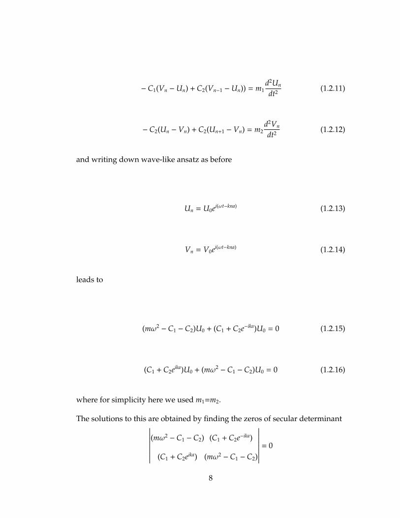
− C1(Vn −Un) + C2(Vn−1 −Un)) = m1d2Un
dt2 (1.2.11)
− C2(Un − Vn) + C2(Un+1 − Vn) = m2d2Vn
dt2 (1.2.12)
and writing down wave-like ansatz as before
Un = U0ei(ωt−kna) (1.2.13)
Vn = V0ei(ωt−kna) (1.2.14)
leads to
(mω2− C1 − C2)U0 + (C1 + C2e−ika)U0 = 0 (1.2.15)
(C1 + C2eika)U0 + (mω2− C1 − C2)U0 = 0 (1.2.16)
where for simplicity here we used m1=m2.
The solutions to this are obtained by finding the zeros of secular determinant∣∣∣∣∣∣∣∣∣∣(mω2
− C1 − C2) (C1 + C2e−ika)
(C1 + C2eika) (mω2− C1 − C2)
∣∣∣∣∣∣∣∣∣∣ = 0
8

which is
ω2 =C1 + C2
m±
1m
√C2
1 + C22 + 2C1C2 cos(ka). (1.2.17)
Figure 1.2.4: Dispersion relation of the 1D chain of two different atoms.
This method can be generalized for more complex three-dimensional materials
and most of the advanced condensed matter textbooks explain this approach
thoroughly. To complete the normal mode solution in three dimensional, the
vibrational amplitude should be incorporated which can be used to calculate
the total energy of the crystal as well.
1.3 Negative thermal expansion
It is not uncommon that some materials show the opposite behavior of PTE,
9

which they shrink upon heating give rise to negative thermal expansion (NTE).
This is relatively new filed of study, yet we have seen phenomenal development
in recent years as many materials are discovered displaying this unusual be-
havior. The most popular example for NTE phenomenon is the liquid water-ice
expansion below 40 C and above ice-water phase boundary.
Even though not all of the different mechanisms responsible for NTE are fully
understood, generally the origin of NTE is viewed in two different ways. NTE
could either arise from non-vibrational effect associated with electronic and
magnetic instabilities or emerge from vibrational effect associated with intrinsic
geometrical instabilities.
1.3.1 Negative thermal expansion from phase competition
The non-vibrational effects account for NTE are mostly related with phase
transitions and one of the very well known example for this type of materials
family is ferroelectrics. Interestingly, some ferroelectrics exhibit NTE or anoma-
lous thermal expansion properties below the curie temperatures and their NTE
originates from ferroelectric order which occurs due to the strong hybridization
between cations and anions. Some of the notable examples in this category are
PbTiO3[2, 25, 26, 27],PbTiO3 based compounds[28, 1], BaTiO3[29], BiFeO3[25],
Pb(Zn1/3Nb2/3)O3[30], Ca3Mn2O7[31], Ca3Ti2O7[31] and Sn2P2S6[32]. The NTE
associated with the spontaneous polarization originating from Pb/Bi-O hy-
bridization is reported for PbTiO3-based compounds [28] and they have at-
10

tracted attention due to the precise capability of controlling NTE, not just in
a single way but by using various methods such as the chemical modifica-
tion, size effect, and physically by applying pressure. A couple of examples of
ferroelectric NTE are shown in Figure 1.3.1.
Figure 1.3.1: NTE in ferroelectrics. (a) Unit cell volume of 0.5PbTiO3-0.5(Bi1−xLax)FeO3 (x = 0.0, 0.1, and 0.2) as function of temperature. FE andPE mean ferroelectric and paraelectric, respectively. Taken from [1]. (b) Ther-mal expansion coefficient of volume in PbTiO3.Taken from [2].
The change of electron configuration can also cause NTE and abnormal thermal
expansion properties to some materials. The volume increment upon cooling
due to a valance transition has been reported for rare earth fulleride Sm2.75C60
[4]. NTE in BiNiO3 [3] is attributed to atomic radius contraction caused by
intermetallic charge transfer from Ni to Bi. Others display NTE due to intersite
charge transfer, as reported in perovskites oxides such as SrCu3Fe4O12[33] and
LaCu3Fe4O12[34]. Even semiconductors (e.g. Si, Ge, and GaAs [35, 36]), su-
perconductors (e.g. MgB2, Ba(Fe0.926Co0.074)2As2 [37, 38]) and Mott insulators
(e.g. Ca2RuO4 based compounds [39, 40] ) exhibit NTE or anomalous thermal
11

expansion properties as a result of change in electron configuration. There exist
a number of ways to tune NTE due to phase competition, including controlling
free electron concentration of semiconductors, modulating the metal insulator
transition of Mott insulator, and introducing quenched disorder. An attribute
of this approach is the potentially large CTE, although a drawback in most
cases is persistence over only a narrow temperature range.
Figure 1.3.2: NTE due to valance transitions. (a)Temperature dependence ofthe unit cell volume of BiNiO3. Low pressure-temperature and high pressure-temperature data are drawn as open and closed circles, and crosses show theweighted average volume in the transition region. From [3]. (b)The dilatomet-ric linear thermal expansion of Bi0.95La0.05NiO3 on heating and cooling showinga 20 K hysteresis. From [3]. (c)Temperature evolution of structure parameterunit cell volume of Sm2.75C60.From[4]
A change in volume in response to staggered or uniform spontaneous magneti-
12

zation is known as magnetovolume effect” has been identified as the cause for
anomalous thermal expansion of magnetic materials. The underlying nature
of NTE or anomalous thermal expansion in magnetic materials is the coupling
between magnetic order and the lattice. The first discovery of low thermal
expansion material of this type happened to be in 1897 by Guillaume and it
was the famous industrial alloy InVar (Fe.64Ni.36) [41]. Since then there are
many known magnetic materials which exhibit NTE include alloys (GdAgMg
[6] ), iron based alloys ( Nd2Fe17Nx[42], Gd2Fe17[43]), oxides ( (La0.8Ba0.2)MnO3
[44]), sulphides(CdCr2S4 [45]), fluorides (perovskite MnF3 [5] ) and nitrides
(antiperovskite manganese alloy based nitrides [46]). These materials display
a variety of unusual mechanical properties such as large, tunable CTE over
a considerable temperature span. An excellent review of NTE in functional
materials can be found in literature [47]
1.3.2 Negative thermal expansion from framework dynamics
Besides NTE from phase competition, there also exists a growing class of mate-
rials with strong, isotropic, robust and thermally persistent NTE that originates
from vibrational mechanism, or in other words intrinsic structural degrees of
freedom. NTE of this type has recently been described as structural negative
thermal expansion (SNTE) [48].
SNTE is a fascinating and growing field of condensed matter physics due
to the rarity of the phenomenon, stunning display of unconventional lattice
13

Figure 1.3.3: NTE in magnetic materials. (a) Temperature dependence of theunit-cell volume of MnF3 . The Neel temperature, TN is shown. From [5]. (b)Relative length changes ∆L/L0 of ferromagnet GdAgMg for various magneticfields. From [6]
dynamics, and strong potential for structural applications where dimensional
stability is required. This type of NTE phenomenon refers to the unusual
tendency for materials to shrink when heated as a property of bond network
topology and the associated fluctuations [49, 50, 51] which is distinct from NTE
arising from electronic or magnetic degrees of freedom described in section
1.3.1.
SNTE is most often discussed in connection with transverse fluctuations of
a linkage between volume defining vertices, which may accompany the libra-
tional (rocking) vibrations in rigid bonds or hindered rotational motion of rigid
polyhedral subunits. The most studied example that shows this type of be-
havior is ZrW2O8 (ZWO) [7, 52, 53, 54, 55, 56]. This cubic material has a large
unit cell, containing 44 atoms in the form of corner linked ZrO6 octahedra and
14

Figure 1.3.4: Negative thermal expansion in ZWO. Filled circles representneutron diffraction data while open circle represent dilatometry data. Takenfrom [7].
WO4 tetrahedra. The NTE behavior is strong (Figure 2.3.9) in ZWO ( αV = -27.3
x 10−6/K up to 400K) compared to most of NTE materials of this class and re-
ported over wide range of temperature range (0.3-1050 K). The ZrO6 octahedra
and WO4 tetrahedra connect via the corner O atom, but one of the O in WO4 is
not connected to another unit and the origin of the NTE comes from transverse
vibration of Zr - O - W bond [57]. At the same time, the NTE in ZWO survives
even after a phase transition occurs at 430 K, but the volumetric thermal expan-
sion coefficient decreases to -18 x 10−6/K. Well-known categories of materials in
which the NTE behavior has been attributed to vibrational mechanisms include
metal cyanides [58], various zeolite frameworks [59], A2M3O12 series [60, 61],
ZWO family[7, 62], ZrV2O7 family[63, 64], Prussian blue analogues[65], MOF-5
materials [66, 67] and metal fluorides [68].
15

1.4 Theoretical consideration of negative thermal expansion
1.4.1 Grneisen theory and thermal expansion
As introduced by Germen Physicist Eduard Grneisen [69, 70], Grneisen theory
assumes that the phonon frequencies of a crystal are modified as the volume
changes. The changing frequencies would allow calculating thermodynamic
functions with in harmonic approximation. This approach is known as quasi-
harmonic approximation. See reference [71] for more details.
Within Grneisen theory, for a crystal with many normal modes, the mode
Grneisen parameter is defined, which explains the effect that changing the vol-
ume of a crystal lattice has on its vibrational properties, and as a consequence,
the effect that changing temperature has on the size or dynamics of the lattice.
Since thermal expansion is a result of the anharmonic nature of bonds, quan-
tification of the anharmonicity in a solid can be achieved with mode Grneisen
parameter, γ(q)i. The mode-dependent Grneisen parameter for a phonon mode
i at a reciprocal lattice point q can be defined as
γ(q)i = −∂ logω(q)i
∂ log V(1.4.1)
where V is the unit cell volume, and ω(q)i is the frequency of the ith mode of
vibration, which itself is a function of a wave vector q in the BZ.
Equation 1.4.1 implies that for a NTE material, γ(q)i is negative, for modes
16

soften with increasing temperature and positive, for modes stiffen with in-
creasing temperature. The overall expansion behavior of a material depends
on the combined contributions from all modes, therefore materials with neg-
ative mode Grneisen parameters are not necessarily NTE materials. Often
thermal expansion is quantified by mean Grneisen parameter, obtained by
integrating Equation 1.4.1 over all modes:
γ = −αVBV
CV(1.4.2)
where B is bulk modulus and CV is constant volume heat capacity. As B,CV,
and V are positive for materials in thermodynamic equilibrium, NTE materials
necessarily possess a negative mean Grneisen parameter.
1.4.2 Rigid unit mode picture
Studies have shown that the lattice vibrations responsible for NTE in ZWO
are in the energy scale of around 2 meV [55, 50, 72, 73]. The bond stretching
and bond bending modes are mostly frozen at this energy scale and vibrations
which respect and maintain internal polyhedral distances and bond angles
have special significance. The WO4 tetrahedral stretching and bending modes
are not thermally excited at the low temperatures where NTE begins, [56]
suggesting a hierarchy of energy scales: stiff bond stretching, intermediate
bond bending, and a set of low- energy external modes of rigid polyhedra
17

units called rigid unit modes (RUMs). The latter set may be supported at low-
energy only in certain regions of reciprocal space which are particular to the
system under consideration.
The RUM model was first used to explain the displacive phase transitions in
silicates [74, 75]. It was developed to describe the behavior of materials with
crystal structures that can be described as frameworks of linked polyhedra
(examples are ScF6 octahedra in ScF3 and WO4 tetrahedra in ZWO). Vallade
and coworkers [76] have shown that the softening of an optical mode nearby
an acoustic phonon causes the phase transition of the material quartz and the
whole phonon branch has a low frequency at each k values, hence must be
associated with RUMs not only at one k value, but along the whole branch.
The idea of RUMs acting as soft modes for displacive phase transition was
later developed for silicates using a split atom method.
The RUM model has given a number of other new insights and most impor-
tantly it has also been used to explain the origin of negative thermal expansion
in framework structures. Phonons described by RUM model are associated
with collective motion of polyhedra and those collective motions cause atomic
displacement without distorting the polyhedra. Therefore these modes are
often identified as NTE modes in SNTE materials. Usually the polyhedra vi-
brational energies are very high when they are distorted compared with the
energy when they are not distorted. As a result, we generally expect RUM
modes to have low energies. For ZWO the manifold of momenta supporting
18

RUMs is very complex, as identified through classical calculations [54] using
split atom approach. Simplest case of RUMs associated NTE is described in
cubic lattice systems ScF3 and ReO3 and more importantly their RUMs corre-
spond to simple momentum space manifolds. ScF3 has only four atoms per
unit cell and forms with corner linked octrahedra of ScF6. High symmetry
points of Brillouin zone (BZ), corresponds to in phase rotation of each stack of
octrahedra (M point) and out of phase rotation of each stack of octrahedra (R
point) defines the boundaries of RUM in ScF3 material. Please see Figure 5.1.1
for a better view on this.
Welches and coworkers have developed a simple qualitative picture explaining
NTE [77] in ReO3 like structures. It is related with geometrical frame work and
is associated with the rotation of stiff structural units or bond bending of the
shared corner atom of the polyhedra units by preserving the rigid unit structure
(RUM). For simplicity the rotation of a 2D perovskite (2D frame work of linked
squares) is considered and the important point is that the area or lattice constant
is reduced by the rotation as a straightforward geometrical effect(Figure 1.4.1).
Considering the potential energy of rotation due to thermal fluctuations,12
Iω2〈θ2〉T =
12
kBT2 where I is the moment of inertia of the units, ω2 is average or Einstein
frequency for the rotations, 〈θ2〉T is the equilibrium fluctuating value of θ2 at
temperature T, kB is Boltzmanns constant. Considering the lattice area reduc-
tion, from A0 to A0 cos2 θ the lattice constant obeys the relation a = a0(1 − ηaθ2)
and the expression∆aa
= −ηakBTIω2 is obtained, which then reduces to CTE
19

Figure 1.4.1: Rotation of 2D perovskite leads to an area reduction.
αL = −ηakB
Iω2 . Here ηa is identified as geometrical constant which is equal to
unity in this case. Chapter 5 discusses a model that we developed to approx-
imate the staggered rotation in 2D square lattice and proves that the above
constant equals to 1/2 in a 2D lattice with few squares, where harmonic wave
limit is applied and 2/3 in a lattice with large number of square units, where
circle wave limit is applied.
As shown the geometrical effect on the CTE leads to a negative CTE. At the
same time since the frequency of modes appears at the bottom of the CTE it
resembles that the softer modes contribute more to the CTE. A particularly
soft dynamic distortion of this structure preserves bond lengths and internal
polyhedral bond angles while decreasing the volume of the time-averaged
structure as the vibrational amplitude is increased through thermal activation.
This classical picture has been widely discussed in general reviews of the NTE
20
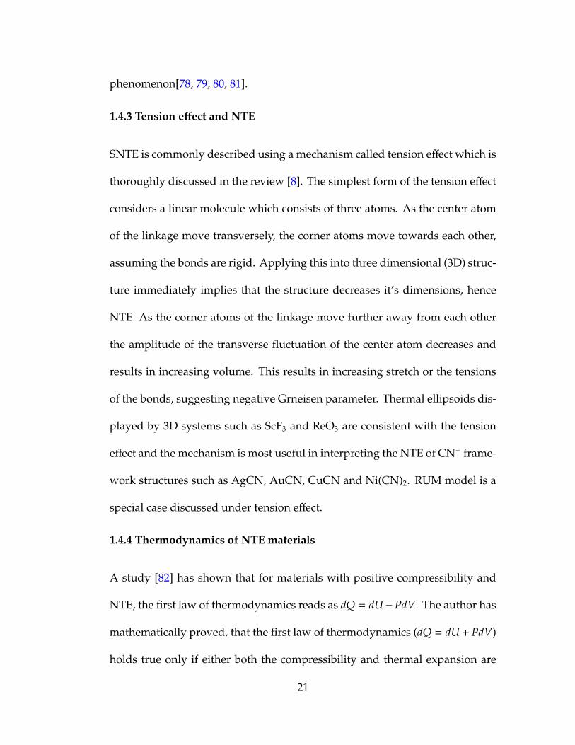
phenomenon[78, 79, 80, 81].
1.4.3 Tension effect and NTE
SNTE is commonly described using a mechanism called tension effect which is
thoroughly discussed in the review [8]. The simplest form of the tension effect
considers a linear molecule which consists of three atoms. As the center atom
of the linkage move transversely, the corner atoms move towards each other,
assuming the bonds are rigid. Applying this into three dimensional (3D) struc-
ture immediately implies that the structure decreases it’s dimensions, hence
NTE. As the corner atoms of the linkage move further away from each other
the amplitude of the transverse fluctuation of the center atom decreases and
results in increasing volume. This results in increasing stretch or the tensions
of the bonds, suggesting negative Grneisen parameter. Thermal ellipsoids dis-
played by 3D systems such as ScF3 and ReO3 are consistent with the tension
effect and the mechanism is most useful in interpreting the NTE of CN− frame-
work structures such as AgCN, AuCN, CuCN and Ni(CN)2. RUM model is a
special case discussed under tension effect.
1.4.4 Thermodynamics of NTE materials
A study [82] has shown that for materials with positive compressibility and
NTE, the first law of thermodynamics reads as dQ = dU−PdV. The author has
mathematically proved, that the first law of thermodynamics (dQ = dU + PdV)
holds true only if either both the compressibility and thermal expansion are
21

Figure 1.4.2: Representation of the tension effect. A linear linkage of threeatoms is shown in left. This can distort such a way that the central atomdisplaces transverse direction or the two end atoms displace in opposite ways.In both cases the bonds stay in rigid and the two end atoms move inwards inthe vertical direction. Taken from [8]
negative or both of them are positive. A different [83] study has proposed
the isentropic (constant entropy) volume expansivity, αV = (1/V)(∂V/(∂T)S
for materials with NTE instead of standard definition of isobaric (constant
pressure) CTE, αV = (1/V)(∂V/(∂T)P.
There are plenty of materials found to be possessing NTE property and thou-
sands of literature have been published directly or indirectly related with NTE
phenomenon, but only a handful numbers of thermodynamic analysis on NTE
materials are found in literature. So readers who are interested would find it
is worth working in this field.
1.5 Perovskites
22

Perovskite oxides, a class of solid materials with chemical formula ABO3, con-
tains examples of perhaps every possible type of material behavior. Underpin-
ning the competing interactions behind this diversity are fascinating cascades
of structural transitions associated with tilts of the BO6 octahedra, which are
strongly influenced by the A-site ions through geometric tolerances[84, 85].
A-site-free perovskites based on oxygen are rare, as the B ion must take on the
extremal +6 valence state, and the only known instance is ReO3. A moderately-
sized NTE effect occurs at low temperature in this material[86] and can be
understood in terms of a model of rigid unit modes (RUMs) described in sec-
tion 1.4.2. Though that is the case with oxides, A site free perovskite fluorides
or in other words MF3-type structures are not rare because of the common
trivalent(+3) state found in most of the metals in the periodic table, especially
among transition metals and lanthenides.
1.6 Trifluorides and their structures
Figure 1.6.1 shows a global structural phase diagram of MF3 perovskites, where
M is a +3 metal ion. For large (rS > 0.85A) ionic radius rS (Shannon), fluorine
ions can pack around the M ion with high F coordination up to n=8 or 9 in com-
mon large-gap optical materials of orthorhombic and tysonite type structures
which are commonly formed with rare earth metal ions.
Order-disorder type second order phase transitions has been reported for LaF3
- NdF3[87] (refer Figure 1.6.1), from low temperature trigonal(P3c1) to high
23

Figure 1.6.1: Global structural phase diagram of MF3 type perovskites.
temperature hexagonal (P63/mmc) phases which both are two modifications
of tysonite type structure[88]. SmF3 - GdF3 crystallize from melt to tysonite
type structure and upon cooling they transform into orthorhombic(Pnma) β-
YF3 [89] type structure. Structural phase transitions occurred in TbF3, DyF3
and HoF3 are accounted for some sort of impurity[90, 91, 92] in the system and
no transition has been reported for pure systems. ErF3 - YbF3, LuF3 and YF3
yield a new high temperature form of α-YF3 type[92].
Below rS < 0.8A, perovskites form with simple-cubic symmetry(Pm3m) at high
temperatures. At low rS, and among the 3d metal trifluorides, a structural
cubic-to-rhombohedral(R3c) phase boundary is apparent, with the exception
24
of MnF3. ScF3 is the only trifluoride with cubic symmetry at room temperature
and can be considered to be the standout among all and will be discussed
thoroughly through out the thesis.
1.7 Scandium trifluoride(ScF3)
1.7.1 Negative thermal expansion in ScF3
Recently, nonmagnetic ionic insulator ScF3 has drawn particularly intense at-
tention in the chemistry community[9] as the first instance of a perovskite-
structured material with strong, isotropic, and thermally persistent NTE, a
distinction which no longer appears to be an isolated case[93]. ScF3 displays
strong NTE (-42 ppm/K < αV < 0) over a temperature window of 1000 K, but is
also unusual in its lack of any type of phase transition whatsoever within the
solid state.
Cubic ScF3 has 4 atoms per unit cell and consists of corner-inked octahedra
which fill space in three dimensions with unit cells a = b = c. The high
symmetry points in the first Brillouin zone (BZ) in reciprocal space are labeled
zone center Γ(0, 0, 0), zone face center X (2π/a(1/2, 0, 0)), zone edge center
M(2π/a(1/2, 1/2, 0)), and zone corner R(2π/a(1/2, 1/2, 1/2)). Sc has the longest
Shannon effective ionic radius of all 3d transition metal trifluorides, and the
lattice dimension parameter a = 4.02 Å at room temperature is very close to
twice the sum of these radii for Sc (0.745 ) and F (1.19 Å), suggesting chemical
25

bonding is ionic.
1.7.2 Pressure induced phase transition in ScF3
Cubic ScF3 further stands out among substances in that it has the most stable
structural phase of any known solid trifluoride, retaining cubic symmetry from
its high melting point >1800 K to <0.5 K[9, 94]. A finite-temperature cubic to
rhombohedral (c-r) transition can be induced however through application of
slight pressure [95, 96] (<0.2 GPa ∼ 2000 atm), chemical substitution of Ti[20],
Al[19], or Y[97] for Sc, and even by the weak stresses induced by polymeric
impregnation of powder samples[21], suggesting that the quantum nature of
the cubic phase at low temperature is delicate and susceptible to even mild
perturbations.
X-ray diffraction [95, 9] and Raman spectroscopy[95] results have revealed
that at room temperature ScF3 undergoes a pressure induced phase transition
from c-r between 0.5 and 0.8 GPa and rhombohedral to orthorhombic structure
above 3.0 GPa. As suggested by the authors[95] the first transition point which
is quite low as hydrostatic pressure is the result of disturbance of the balance
between short-range dipoledipole(of fluorine ions) and long-range Coulomb
interactions which is related to rotation of the ScF6 octahedra around a threefold
axis. The rotation of octahedra corresponds to R = π/a(1, 1, 1) point in cubic
phase BZ and the c-r phase transition occurs due to condensation of this mode
(Figure 1.7.1).
26

Observed pressure dependence of the transition temperature is dTc/dp ∼ 525
K/GPa [9, 95, 96]. The c-r phase transition in ScF3 is never realized down to 0.4
K [94] in atmospheric pressure and using inelastic x-ray scattering (Chapter:2)
results, we estimate that pressures as small as 740 bar = 0.074 GPa would be
sufficient to drive the transition upward to 0 K. The sensitivity of the phase
boundary suggests that the nature of the cubic phase is delicate at low temper-
ature and susceptible to even mild perturbations [21, 20, 20, 19]. Section 2.3.10
further discusses this.
If suitable substrates of ScF3 are developed, new functionalities may be reached
in film synthesis, as cooling from the growth temperature would effectively
stretch epitaxial films. Significant efforts in the physics groups of Profs. Barrett
Wells in Physics Department have already produced thin films of NTE ScF3
[98]. Thin films of ScF3 are grown using pulsed laser deposition, and while
large fraction of a film is having very good epitaxy and small mosaic, remaining
regions are polycrystalline. Unique features of this material such as large band
gap, non-oxide nature, poor adhesion under pressure and high saturated vapor
pressure remain as significant challenges to overcome.
1.7.3 Electronic structure of ScF3
In formation of ScF3, from a scandium atom and a fluorine atom, the scandium
atom loses its three valence electrons (and turn to Sc+3 ) to three fluorine atoms
(and form F−), which each of the fluorine has just enough space to accept it. We
27
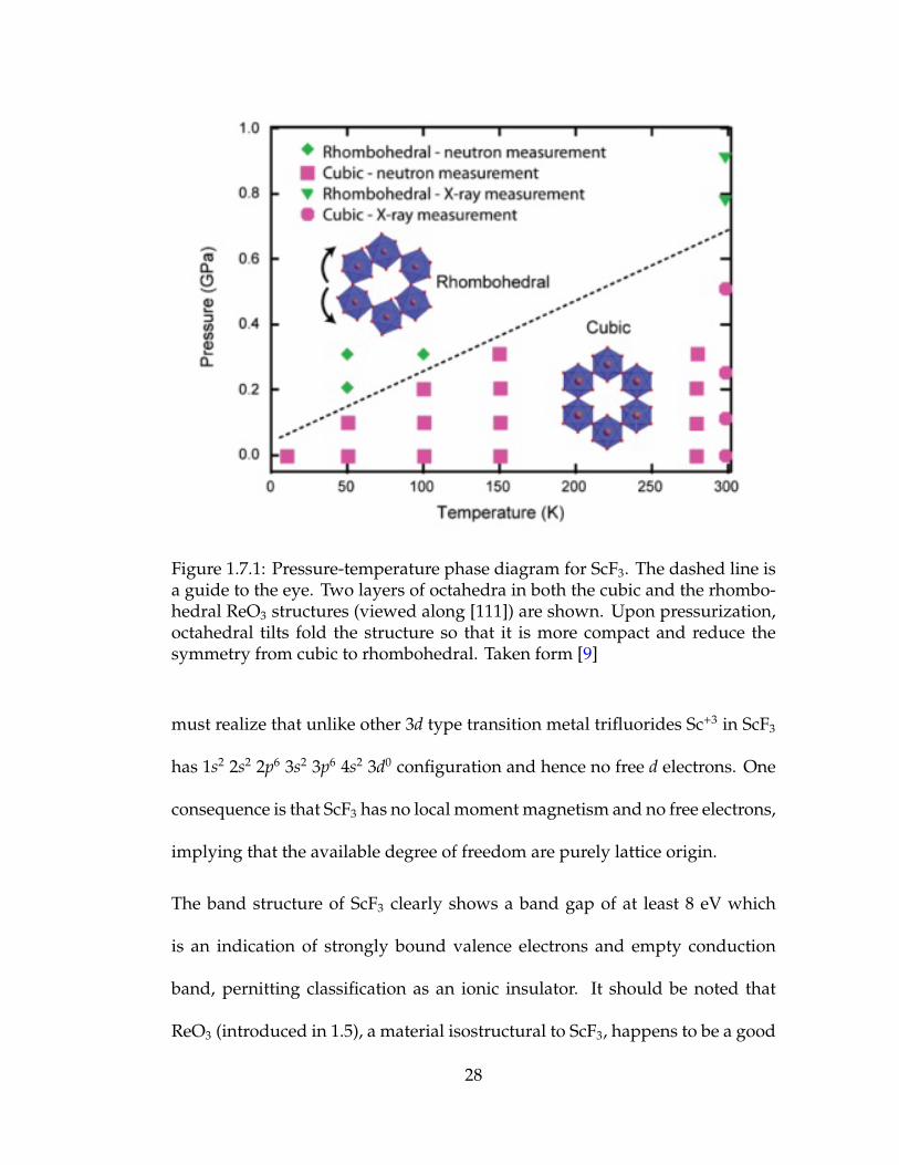
Figure 1.7.1: Pressure-temperature phase diagram for ScF3. The dashed line isa guide to the eye. Two layers of octahedra in both the cubic and the rhombo-hedral ReO3 structures (viewed along [111]) are shown. Upon pressurization,octahedral tilts fold the structure so that it is more compact and reduce thesymmetry from cubic to rhombohedral. Taken form [9]
must realize that unlike other 3d type transition metal trifluorides Sc+3 in ScF3
has 1s2 2s2 2p6 3s2 3p6 4s2 3d0 configuration and hence no free d electrons. One
consequence is that ScF3 has no local moment magnetism and no free electrons,
implying that the available degree of freedom are purely lattice origin.
The band structure of ScF3 clearly shows a band gap of at least 8 eV which
is an indication of strongly bound valence electrons and empty conduction
band, pernitting classification as an ionic insulator. It should be noted that
ReO3 (introduced in 1.5), a material isostructural to ScF3, happens to be a good
28

metal. The vastly different electronic structures of otherwise similar materials
might be interesting to further investigate.
Since both materials are SNTE materials, it is meaningful to compare the elec-
tronic structures of each with its own distorted structure. Using first principle
calculations, a comparative study [99] has been carried out and the electronic
band structure of distorted ReO3 (O atoms are displaced perpendicular to Re-
O-Re bond) has shown a small destabilization of the flat conduction band
compared with conduction band of non-distorted structure. The atomic dis-
placement was attributed to formation of antibonding orbitals and the authors
conclude that this results in destabilizing the distortion of ReO3 structure. On
the other hand the electronic band structure of distorted ScF3 structure hardly
changes from its non distorted counterpart. Therefore it is concluded that the
ScF3 favors the distortion more than that of ReO3 and as a result the CTE of
ScF3 (αV = -42x10−6/K in 60 K to 110 K temperature window and ∼ -25x10−6/K
at 300 K) is larger than ReO3 (αV = -7.68x10⁻⁶/K in 5 K to 300 K temperature
range).
1.8 Motivation
A central question in the study of SNTE is whether basic structural mechanics
principles and intuition can be applied to guide discovery of new materials
that display this anomalous effect. For example, metallic ReO3 and insulating
ScF3 with open perovskite structure display SNTE over a wide range of tem-
29

peratures, but why do other open perovskites most commonly exhibit positive
thermal expansion (PTE)? or can composite materials be formed with thermal
expansion over a wide temperature window, or do stresses inevitably shift the
structural phase to one with PTE? Why is SNTE so rare, inevitably yielding to
PTE in response to disorder and application of pressure?
In pursuit of conceptual control of the phenomenon, innovative approaches
have been offered which link thermally activated transverse vibration of struc-
tural units to a tendency to draw in lattice dimensions. Rigid unit approaches
view polyhedral molecular units (i.e., metal-anion tetrahedra and octahedra)
rather than ions as the fundamental building blocks of a material and attempt
to link the states built from rotational zero modes of the free molecules to the
low-energy modes of the crystal. In this view, intramolecular degrees of free-
dom are effectively integrated out, and the nature of their coordinated motion
as a function of lattice topology and connectivity is the central feature of SNTE.
New discoveries of robust SNTE have reinvigorated the field and raised the
question of whether strict molecular rigidity is an appropriate starting point
or if, instead, it is more appropriate to consider only the rigidity of the stiffest
bonds in a view of the materials as a framework of struts.
30
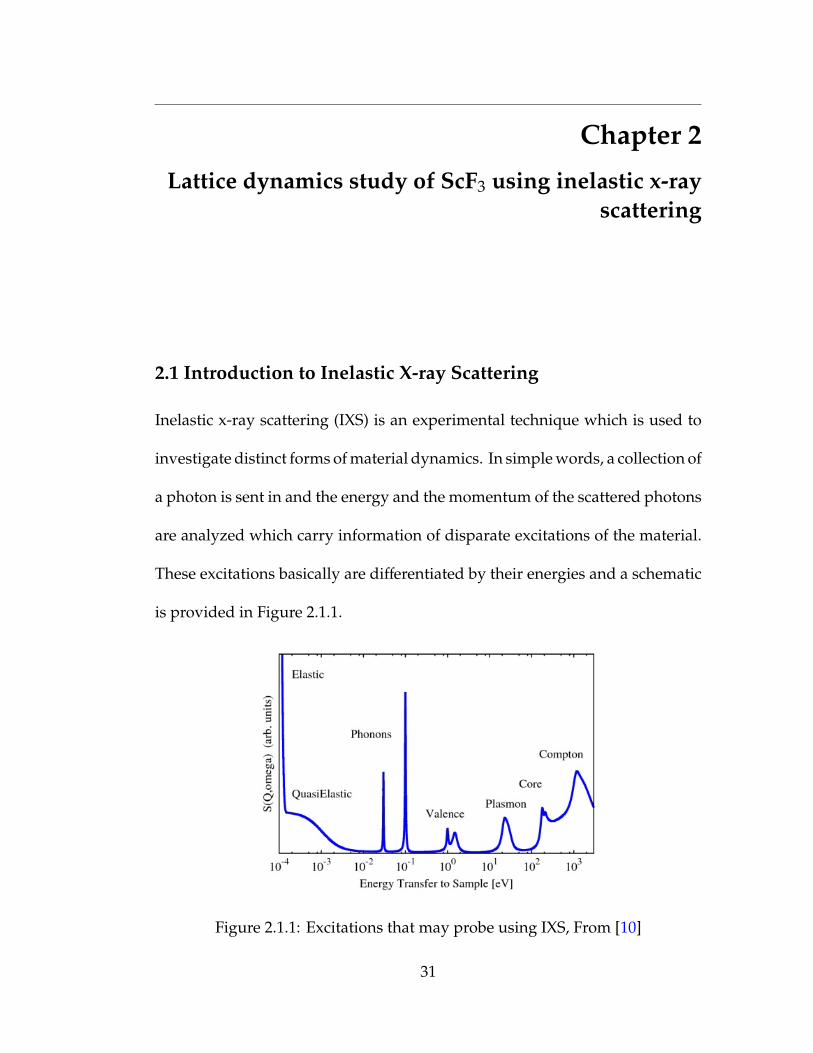
Chapter 2
Lattice dynamics study of ScF3 using inelastic x-rayscattering
2.1 Introduction to Inelastic X-ray Scattering
Inelastic x-ray scattering (IXS) is an experimental technique which is used to
investigate distinct forms of material dynamics. In simple words, a collection of
a photon is sent in and the energy and the momentum of the scattered photons
are analyzed which carry information of disparate excitations of the material.
These excitations basically are differentiated by their energies and a schematic
is provided in Figure 2.1.1.
Figure 2.1.1: Excitations that may probe using IXS, From [10]
31

We can identify several distinct methods used in order to probe those excitations
and since there are no sharp boundaries among excitations energies, some of
them may be probed using more than one technique. Table 2.1.1 lists some of
the techniques that fall under the broad interpretation of the IXS.
Technique Incidentphotonenergy
Energy transfer Information ofthe material
—————————-————— ————————————————Compton 100 keV keV Electron momen-
tum densityMagnetic Compton 100 keV eV Density of un-
paired spinRIXS(Rasonance) 4-20 keV 0.1 - 50 eV Electron structure
and excitationsSIXS(Soft x-ray) 0.1-2 keV 0.01 - 5 eV Electronic and
magnetic struc-ture and excia-tions
NIS(Nuclear IXS) 10-30 keV 1 - 100 meV Element specificphonon andDensity of state(DOS)
X-ray Ramam 10 keV 50 - 1000 meV Edge structure,Bonding, Valence
NRIXS 10 keV 0.01 - 10 eV Electronic struc-ture and excita-tion
IXS 10-25 keV 1 - 100 meV Atomic dynamicsand phonon dis-persion
Table 2.1.1: List of techniques broadly grouped under the heading of InelasticX-Ray Scattering.From[10]
2.1.1 IXS advantages over other spectroscopic techniques
One of the significant advantages of IXS is the access to small samples. The
32

synchrotron radiation of high flux and brilliance is capable of focusing the
beam to ∼ 100 microns diameter easily. Even ∼ 10 microns in diameter can
be achieved with some losses. The facts that incoming x-ray photon energy
of ∼ 20 keV is significantly higher than the measured energy transfer of ∼
1-200 meV and the energy and momentum of photon is directly proportional
to each other lead to other compelling advantageous of using IXS such as
decoupling of the energy and momentum transfer, achieving high momentum
resolution and independence of energy resolution from energy transfer. The
Thompson cross section for x-rays is smaller than the absorption scattering
cross section at least by one order of magnitude. This could prevent multiple
scattering from the sample and incoherent scattering at higher energies by only
penetrating into the top 0.01 or 0.1 mm of the sample. Therefore most materials
have very short attenuation length for x-rays which eventually results in lower
background signal as well. But in case of neutron, the scattering cross section
dominates hence multiple scattering can be a problem. On the other hand
higher absorption cross section in x-rays could easily leads to radiation damage
of the material. Nevertheless, it is worthwhile to mention that neutron holds
the edge when higher energy resolution is needed but some of the samples can’t
be measured using neutron scattering or diffraction experiments as they highly
absorb neutrons. Some of the common examples are Cadmium, Samarium and
Europium.
Next section in current chapter is dedicated to elaborate general scattering
33
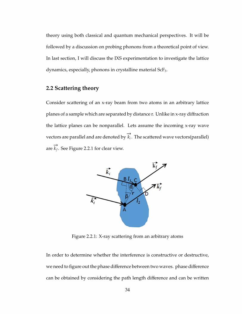
theory using both classical and quantum mechanical perspectives. It will be
followed by a discussion on probing phonons from a theoretical point of view.
In last section, I will discuss the IXS experimentation to investigate the lattice
dynamics, especially, phonons in crystalline material ScF3.
2.2 Scattering theory
Consider scattering of an x-ray beam from two atoms in an arbitrary lattice
planes of a sample which are separated by distance r. Unlike in x-ray diffraction
the lattice planes can be nonparallel. Lets assume the incoming x-ray wave
vectors are parallel and are denoted by−→ki . The scattered wave vectors(parallel)
are−→k f . See Figure 2.2.1 for clear view.
Figure 2.2.1: X-ray scattering from an arbitrary atoms
In order to determine whether the interference is constructive or destructive,
we need to figure out the phase difference between two waves. phase difference
can be obtained by considering the path length difference and can be written
34

as
∆l = l2 − l1. (2.2.1)
From triangle ABC,
l1 = |−→r | sin(β) = |−→r | sin(90 − α) = |−→r | cos(α) (2.2.2)
and using vectors we may write
−→ki .−→r = |
−→ki ||−→r | cos(α). (2.2.3)
Since
|ki| =2πλ
(2.2.4)
−→ki .−→r =
2πλ|−→r | cos(α) (2.2.5)
l1 =λ
2π−→ki .−→r . (2.2.6)
35
Likewise from triangle ACD,
l2 =λ
2π−→k f .−→r . (2.2.7)
Therefore the path length difference can be written as
∆l =λ
2π(−→k f −−→ki ).−→r (2.2.8)
and the phase difference is given by
∆l2πλ
= (−→k f −−→ki ).−→r =
−→Q.−→r (2.2.9)
here−→Q is defined as scattering vector where,
−→Q =
−→k f −−→ki (2.2.10)
The scattering wave vector,−→Q and the spatial arrangement of the atoms in the
sample are key factors when determining the signal at the detector. The spatial
positioning of atom is important since it determines the tendency of sample to
scatter the incoming wave. We can introduce the density of scattering atoms
in the sample to be ρ(−→r ) and assume the scattering density depends on the
36

spatial arrangement of atoms.
Figure 2.2.2: Radiation from source (S) to detector (D) via the sample
Using plane wave approximation and incorporating all above variables, an
expression for the amplitude of the signal at the detector(scattering wave aml-
pitude), fD from a wave emitted by point at tip of the −→r can be written as,
fD ∝ ρ(−→r )ei(−→ki−−→k f ).−→r (2.2.11)
fD ∝ ρ(−→r )e−i−→Q.−→r (2.2.12)
This is specifically derived for one particular point in the sample. Therefore to
calculate the total amplitude at detector we need to integrate over the sample
volume.
37

fD ∝
∫Vρ(−→r )e−i
−→Q.−→r d−→r (2.2.13)
where V is the total volume of the sample.
Fourier transformation of scattering density leads to the expression
ρ(−→Q) =
∫ρ(−→r )e−i
−→Q.−→r d−→r (2.2.14)
which is similar to the amplitude of the signal at the detector.
To describe the scattering density within one unit cell let us assume the atoms
in the unit cell don’t interact with each other and have their own local scattering
density ρ j(−→r′ ) where
−→r′ = −→r − −→r j (2.2.15)
Figure 2.2.3: Reflection geometry where the blue solid circle represents the jth
atom where −→r j and −→r initiate at the unit cell origin
38
The total scattering density
ρ(−→r ) =∑
j
ρ j(−→r − −→r j ) (2.2.16)
Now rewriting the total scattering, plugging ρ j(−→r′ ) and multiplying by 1 =
ei−→Q.−→r j e−i
−→Q.−→r j
ρ(−→Q) =
∑j
ei−→Q.−→r j
∫ρ(−→r′ )ei
−→Q.−→r′d−→r′ (2.2.17)
Here the integral term is known as atomic form factor f j(−→Q) which is a property
of atoms themselves and the summation term∑
j ei−→Q.−→r j depends on where the
atoms are located in the lattice. Finally the intensity of scattered beam is given
by
S(−→Q) = 〈|ρ(
−→Q)|2〉 =
∑j,k
f j(−→Q) fk(
−→Q)〈ei
−→Q.(−→r j−
−→rk )〉 (2.2.18)
which is termed as static structure factor.
2.2.1 Dynamic structure factor (S(−→Q, ω))
In previous section I have formulated a mathematical expression described
scattering from arbitrary atoms instantaneously at a given time. But we can ex-
tend our analysis further to consider scattering from sample atoms at different
39

times. This of course, results in a phase shift in the scattering wave.
Redefining the scattering density in momentum space and introducing phase
shift e−iωt,
ρ(−→Q, t) =
∑j
f j(−→Q)ei(
−→Q.−→r j(t)−ωt) (2.2.19)
Averaging all time to get the total scattering
ρ(−→Q, ω) =
∫ρ(−→Q, t)e−iωtdt (2.2.20)
Writing the intensity of the scattering
S(−→Q, ω) =
∫ρ(−→Q, t′)e−iωt′dt′x
∫ρ(−−→Q, t)e−iωtdt (2.2.21)
Shifting t by t + t′
S(−→Q, ω) =
∫ ∫ρ(−→Q, t′)ρ(−
−→Q, t + t′)e−iωtdtdt′ (2.2.22)
Performing an average over all time origins
S(−→Q, ω) =
∫〈ρ(−→Q, 0)ρ(−
−→Q, t)〉e−iωtdt (2.2.23)
40
Substituting back from Equation 2.2.19
S(−→Q, ω) =
∑j,k
f j(−→Q) fk(
−→Q)
∫〈ei−→Q.−→r j(0)e−i
−→Q.−→r k(t)
〉e−iωtdt (2.2.24)
This is a critical equation in IXS which carries both spatial and time evolution
information about excitations of the system and known as dynamical structure
factor. More importantly for us the signal or the spectra collected in IXS
experiment is directly proportional to dynamic structure factor(S(−→Q, ω)) of the
material.
2.2.2 Quantum mechanical perspective
Let me start by considering the electron-photon interaction Hamiltonian. Con-
ventionally it can be separated into two terms H0 and Hi, where non interacting
term reads
H0 =∑
j
12m−→p j
2 +∑
j, j′V(r j j′) (2.2.25)
and electron - photon interaction term is given by
Hi =∑
j
e2
2mc2
−→A2(−→r j ) −
emc−→A(−→r j ).
−→p j (2.2.26)
While−→A and V denotes the electromagnetic field vector and scalar potentials,
41
the electron momentum and position are denoted by−→p and−→r . In Hamiltonian,
Hi the first terms with A2 term dominates in nonresonant scattering processes
while the second term leads in resonant scattering (case where the incoming
energy is tuned into absorption edge of the atom). The nonresonant scattering
cross section depends on dynamic structure factor and has the form of Equation
2.24. Since we only deal with nonresoannt scattering, from here onwards I
would only take H(1)i =
∑j
e2
2mc2
−→A2(−→r j ) term into consideration.
Introducing the photon creation (a†kα) and annihilation (akα) operators the vector
potential can be written as
−→A(−→r ) = L−3/2
∑k,α
( ~ωk
)1/2c(εαa†kαei
−→k .−→r + εαakαe−i
−→k −→r ) (2.2.27)
where ωk, α and k denote the angular frequency, polarization and wave vector
of photon respectively. L3 is normalization box volume.
Let us now consider photon in three dimensional box of side L. The photon
states are quantized and only allowed k values given by 2π/L(nx,ny,nz) where
nx, ny and nz are integers.
Any possible final-state wave-vector k corresponds to a point in wave vector
space with coordinates (kx, ky, kz). Then we can define the density of k states
(number of k points per unit volume) to be L3/(2π)3. In three dimensional
system the k space volume between k′ and k′ + dk′ is 4π2k′2dk′. Therefore the
number of k states in the region between k′ and k′ + dk′ is
42
( L2π
)34πk′2dk′ (2.2.28)
Hence the number of points for k-vectors going into an element of solid angle
dΩ (Solid angle of sphere is 4π) for polarization state α with energies between
E′ and E′ + dE′ is
( L2π
)3k′2dk′dΩ (2.2.29)
Defining the density of state per unit energy g(E′), where E′ = ~ck′ is the energy
corresponding to wave vector k′ the total number of states between photon
energies E′ and E′ + dE′ could be written as
g(E′)dE′ =( L2π
)3k′2dk′dΩ (2.2.30)
g(E′) =( L2π
)3(k′2
~c
)dΩ (2.2.31)
Normalization corresponds to one particle per box volume L3, so the number
of particles crossing per unit area per unit time is given by the incident photon
velocity divided by the L3 which is defined as the incident flux
43

Incident flux =c
L3 (2.2.32)
Consider scattering process from photon initial state (kα) to final state (k′α′)
and sample intial state λ to sample final state λ′. Using the Fermi golden rule
the rate of transition of scattered flux into solid angle dΩ can be written as
Scattered flux =2π~|〈k′α′λ′|H(1)
i |kαλ〉|2 L3
8π3
k′2
~cdΩ (2.2.33)
Then the differential cross section to solid angle dΩ can be defined as (The cross
section will be elaborated in section 2.2.3)
dσdΩ
=Scattered fluxIncident flux
= |〈k′α′λ′|H(1)i |kαλ〉|
2 L6
4π2
k′2
~2c2 (2.2.34)
Substituting for |H(1)i |,
〈k′α′λ′|H(1)i |kαλ〉 =
1L3
e2
mc2
~c(ωkωk′)1/2 (ε∗α.εα′)〈λ
′|
∑j
e−i(−→k −−→k′ ).−→r j )|λ〉 (2.2.35)
Using ω = ck and considering the energy conservation condition for the scat-
tering process, we obtain the partial differential cross section
44

d2σdΩdE
=( e2
mc2
)2 k′
k|ε1 ∗ ε2|
2〈λ|
∑j
e−i(−→k −−→k′ ).−→r j )|λ′〉〈λ′|
∑j′
ei(−→k −−→k′ ).−→r j′ )|λ〉δ(Eλ−Eλ′ + ~ω)
(2.2.36)
Here wave vector −→q =−→k −−→k′ and taking sum over all possible final state λ′
d2σdΩdE
=k′
kr2
e |ε1 ∗ ε2|2S(−→Q, ω) (2.2.37)
where
S(−→Q, ω) =
∑λλ′
∑j j′
pλ〈λ|∑
j
e−i−→Q.−→r j |λ′〉〈λ′|
∑j′
ei−→Q.−→r j′ |λ〉δ(Eλ − Eλ′ + ~ω) (2.2.38)
and pλ is the probability of initial state λ.
Time dependency To introduce the time dependency, let us write down the
delta function in its integral representation
δ(Eλ − Eλ′ + ~ω) =1
2π~
∫∞
−∞
ei(Eλ′−Eλ)t/~e−iωtdt (2.2.39)
Writing down the wave function in Schrodinger representation
|ψ(t)〉 = U(t)|ψ(0)〉 (2.2.40)
45

where
U(t) = e−iHt/~ (2.2.41)
and the matrix element of the operator can be written as
〈ψ(0)|A|ψ(0)〉. (2.2.42)
In this representation, operators are constants and all the time dependence is
carried by the states. Now defining the operator in Heisenberg picture, in
which the operators carry the time dependency,
A(t) = U(t)†AU(t) (2.2.43)
it is obvious that A(0) = A.
Let us go back to our derivation. Introducing two operators A, A′ and consid-
ering Equation 2.2.39 we can write,
46

∑λ′
〈λ|A|λ′〉〈λ′|A′|λ〉δ(Eλ − Eλ′ + ~ω)
=1
2π~
∫∞
−∞
∑λ′
〈λ|A|λ′〉〈λ′|A′|λ〉ei(Eλ′−Eλ)t/~e−iωtdt (2.2.44)
Applying the operations e−iEλt/~|λ〉 = e−iHt/~
|λ〉 to previous equation
∑λ′
〈λ|A|λ′〉〈λ′|A′|λ〉δ(Eλ − Eλ′ + ~ω) =1
2π~
∫∞
−∞
e−iωtdt∑λ′
〈λ|A|λ′〉〈λ′|A′(t)|λ〉
(2.2.45)
Using the completeness property over sum over λ′ we can write
∑λ′
〈λ|A|λ′〉〈λ′|A′|λ〉δ(Eλ − Eλ′ + ~ω) =1
2π~
∫∞
−∞
e−iωtdt〈λ|A(0)A′(t)|λ〉 (2.2.46)
Using Equation 2.2.46 we can write Equation 2.2.38 as
S(−→Q, ω) =
12π~
∫∞
−∞
e−iωtdt〈ρ(−→Q, 0)ρ†(
−→Q, t)〉 (2.2.47)
Taking the sum over all electrons j, the density fluctuation operator is defined
by
ρ(−→Q) =
∑j
e−i−→Q.−→r j (2.2.48)
47

which is the Fourier transformation of electron density operator
ρ(−→r ) =∑
j
δ(−→r − −→r j ). (2.2.49)
It is worthwhile to note that we can obtain an expression for static structure
factor S(−→Q) simply by integrating the dynamic structure factor (Equation 2.2.47)
over transfer energy ω
S(−→Q) = ~
∫∞
−∞
S(−→Q, ω)dω (2.2.50)
2.2.3 Scattering cross section
The cross section is a quantification of an effective area in which the scattering
event occurs and denoted by σ. In scattering experiments, one is often inter-
ested in knowing how likely a given event occurs. However, the scattering rate
depends strongly on experimental variables such as the density of the target
material, the intensity of the beam, or the area of overlap between the beam
and the target material. To control for these differences, one can factor out these
variables, resulting in an area-like quantity known as the cross section.
The cross section is a scalar that only quantifies the intrinsic rate of an event.
In contrast, the ”differential cross section” dσ/dΩ is a function that quantifies
the intrinsic rate at which the scattered projectiles can be detected at a given
48

angle (where Ω represents solid angle). The total cross section σwould simply
be the integral of dσ.
The cross-section for non-resonant scattering from a material is usually divided
into the product of a term relating to the probe-sample interaction and the
dynamic structure factor, S(−→Q, ω), which is more directly related to atomic
motions in the sample. Scattering rate of photons from incident beam (from
initial state) to scattered beam (to final state) scattered into solid angle dΩ
within energy width dE and momentum transfer−→Q is given by
d2σdΩdE
=k2
k1r2
e |ε1 ∗ ε2|2S(−→Q, ω) (2.2.51)
where k1 and k2 are incident and scattered momentum states of the photons
and ε1,ε2 are corresponding polarization states. Photon has usual energy mo-
mentum relationship of E = ~ωph = ~c|−→k | = ~c/λ. Thompson scattering cross
section or scattering by free electrons ((dσ/dΩ)Th) is defined as r2e |ε1 ∗ ε2|
2 where
re = e2/mec2 is classical electron radius.
2.2.4 IXS for phonons
Inelastic neutron scattering (INS) has long been the method for studying the
lattice dynamics of crystals. As introduced earlier in the chapter, IXS is a key
technique, which could replace the INS since significant recent development of
synchrotron-related instrumentation. Fundamentally they are different as IXS
49
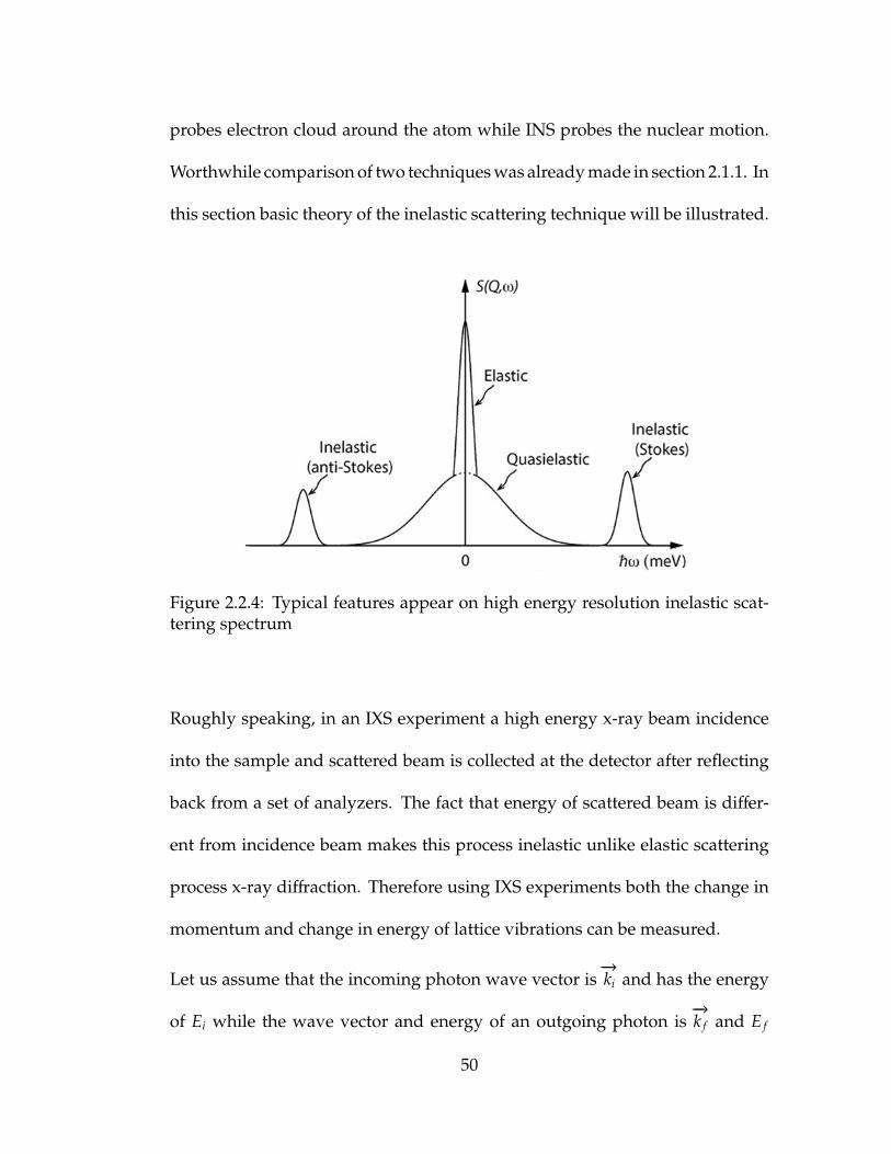
probes electron cloud around the atom while INS probes the nuclear motion.
Worthwhile comparison of two techniques was already made in section 2.1.1. In
this section basic theory of the inelastic scattering technique will be illustrated.
Figure 2.2.4: Typical features appear on high energy resolution inelastic scat-tering spectrum
Roughly speaking, in an IXS experiment a high energy x-ray beam incidence
into the sample and scattered beam is collected at the detector after reflecting
back from a set of analyzers. The fact that energy of scattered beam is differ-
ent from incidence beam makes this process inelastic unlike elastic scattering
process x-ray diffraction. Therefore using IXS experiments both the change in
momentum and change in energy of lattice vibrations can be measured.
Let us assume that the incoming photon wave vector is−→ki and has the energy
of Ei while the wave vector and energy of an outgoing photon is−→k f and E f
50

respectively.
Ei = ~ωi,E f = ~ω f (2.2.52)
The change in energy can be written as
∆E = E f − Ei = ~ω f − ~ωi (2.2.53)
Change in energy of photons can be related to two processes occur inside the
crystal named phonon creation where E f > Ei and phonon annihilation where
E f < Ei. Therefore the difference in energies can be considered as phonon
energy, ~ωph. Likewise, considering the momentum conservation within the
system (Crystal and interactive photons), phonon-created has momentum−→ki −
−→k f ±
−→G and phonon-annihilated has momentum of
−→k f −
−→ki ±
−→G , where
−→G is
reciprocal lattice vector of the crystal. Please refer the Figure 2.2.5.
Figure 2.2.5: Phonon creation is shown on left and phonon annihilate processon right
2.2.5 Scattering from phonons in theoretical perspective
In the derivation of section 2.2.2 we assumed that the x-ray energy transfer is
51
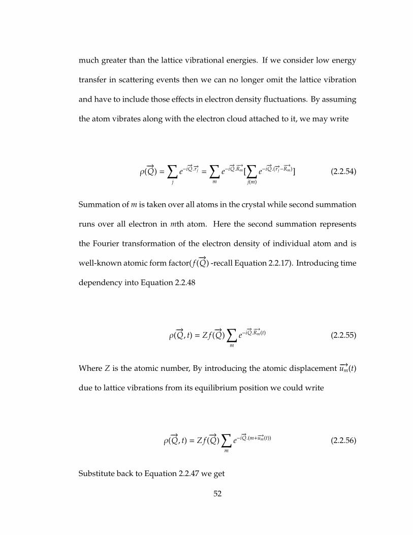
much greater than the lattice vibrational energies. If we consider low energy
transfer in scattering events then we can no longer omit the lattice vibration
and have to include those effects in electron density fluctuations. By assuming
the atom vibrates along with the electron cloud attached to it, we may write
ρ(−→Q) =
∑j
e−i−→Q.−→r j =
∑m
e−i−→Q.−→Rm[
∑j(m)
e−i−→Q.(−→r j−
−→Rm)] (2.2.54)
Summation of m is taken over all atoms in the crystal while second summation
runs over all electron in mth atom. Here the second summation represents
the Fourier transformation of the electron density of individual atom and is
well-known atomic form factor( f (−→Q) -recall Equation 2.2.17). Introducing time
dependency into Equation 2.2.48
ρ(−→Q, t) = Z f (
−→Q)
∑m
e−i−→Q.−→Rm(t) (2.2.55)
Where Z is the atomic number, By introducing the atomic displacement −→um(t)
due to lattice vibrations from its equilibrium position we could write
ρ(−→Q, t) = Z f (
−→Q)
∑m
e−i−→Q.(m+−→um(t)) (2.2.56)
Substitute back to Equation 2.2.47 we get
52

S(−→Q, ω) =
Z2
2π~f 2(−→Q)
∫∞
−∞
e−iωtdt∑m,m′〈e−i
−→Q.−→Rm(0)e−i
−→Q.−→Rm(t)〉
=Z2
2π~f 2(−→Q)
∑m,m′
ei−→Q.(m−m′)
∫∞
−∞
e−iωtdt〈e−i−→Q.−→um(0)ei
−→Q.−−→um′ (t)〉
(2.2.57)
Now let us expand the phonon displacement um(t) in terms of the corresponding
time dependent phonon creation and annihilation operators to obtain
um(t) =∑−→Q0,ε
e(−→Q0, ε)
( ~
2NMω−→Q0,ε
)1/2(α−→Q0,ε
e−iω−−→Q0 ,ε
t+ α†−→
Q0,εeiω−−→
Q0 ,εt) (2.2.58)
where phonon creation operator is α†−→Q0,ε
(t) = α†−→Q0,ε
eiω−−→Q0 ,ε
t and phonon annihi-
lation operator is α−→Q0,ε(t) = α−→Q0,ε
e−iω−−→Q0 ,ε
t. Here−→Q0 and ε denotes the phonon
wave vector and the polarization vector respectively. ω−→Q0,εis phonon angular
frequency. e(−→Q0, ε) is phonon eigen vector and N is total number of atoms in
the crystal.
Manipulating the thermal average exponential using BakerHausdorff theorem
we can obtain the expression. (Of course I do not work out the detailed
derivation here and anyone who is interested can refer the article [100])
〈e−i−→Q.−→um(0)ei
−→Q.−−→um′ (t)〉 = e−〈(
−→Q.−→um(t))2
〉e〈(−→Q.−→um(0))(
−→Q.−−→um′ (t))〉 (2.2.59)
where we define Debye-Waller factor e−2W as
53
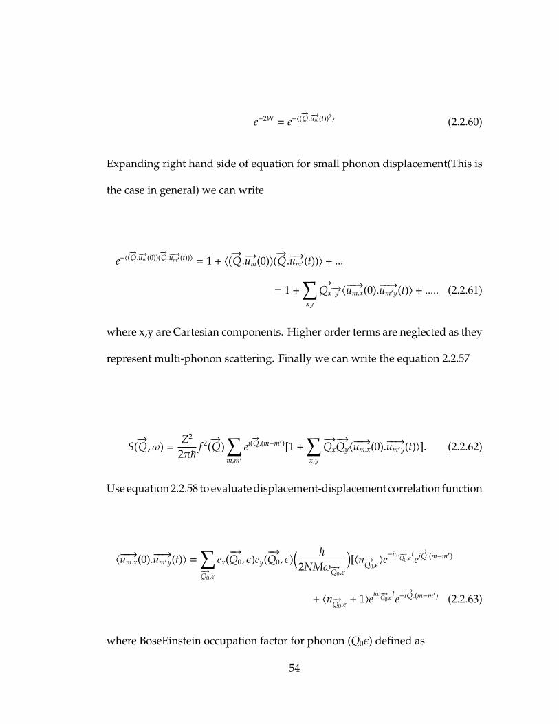
e−2W = e−〈(−→Q.−→um(t))2
〉 (2.2.60)
Expanding right hand side of equation for small phonon displacement(This is
the case in general) we can write
e−〈(−→Q.−→um(0))(
−→Q.−−→um′ (t))〉 = 1 + 〈(
−→Q.−→um(0))(
−→Q.−→um′(t))〉 + ...
= 1 +∑
xy
−→Qx−→y 〈
−−→um.x(0).−−→um′y(t)〉 + ..... (2.2.61)
where x,y are Cartesian components. Higher order terms are neglected as they
represent multi-phonon scattering. Finally we can write the equation 2.2.57
S(−→Q, ω) =
Z2
2π~f 2(−→Q)
∑m,m′
ei(−→Q.(m−m′)[1 +
∑x,y
−→Qx−→Qy〈−−→um.x(0).−−→um′y(t)〉]. (2.2.62)
Use equation 2.2.58 to evaluate displacement-displacement correlation function
〈−−→um.x(0).−−→um′y(t)〉 =
∑−→Q0,ε
ex(−→Q0, ε)ey(
−→Q0, ε)
( ~
2NMω−→Q0,ε
)[〈n−→Q0,ε
〉e−iω−−→Q0 ,ε
tei−→Q.(m−m′)
+ 〈n−→Q0,ε+ 1〉eiω−−→
Q0 ,εte−i−→Q.(m−m′) (2.2.63)
where BoseEinstein occupation factor for phonon (Q0ε) defined as
54
〈n−→Q0,ε〉 =
1eβωQ0 ,ε − 1
. (2.2.64)
Using the definition of delta function,
∑m
ei−→k .−→m =
L3
(2π)3
∑G
δ(−→K −−→G) (2.2.65)
we obtain the final expression for scattering from lattice vibrations
S(−→Q, ω) =
Z~
f 2(−→Q)e−2W L3
(2π)3 [∑
G
δ(−→Q −−→G)]δ(ω) + Z2 f 2(
−→Q)e−2W L3
(2π)3
×
∑−→Q0,ε
12MωQ0,ε
|−→Q.−→e (Q0ε)|2(〈n−→Q0,ε
〉δ(ω + ωQ0,ε) + 〈n−→Q0,ε+ 1〉δ(ω − ωQ0,ε))
× δ(−→Q ±−→Q0 −
−→G). (2.2.66)
Here the first term represents the elastic scattering. Second term represents one-
phonon inelastic scattering with energy gain (phonon annihilation) and one-
phonon inelastic scattering with energy loss (phonon creation) respectively.
Multi-phonon scattering are represented by higher order terms. They are
small in general unless the temperature is very high and omitted as stated in
the middle of the derivation process.
2.3 Inelastic X-ray Scattering on ScF3
55

2.3.1 The Experiment
In order to study the lattice dynamics of ScF3, which has a simple cubic unit
cell (Figure 2.3.1) of space group Pm3m the experiment was performed in the
HERIX (High energy resolution inelastic x-ray scattering) beam line (Sector 30)
at Advanced Photon Source(APS) at Argonne National Laboratory(ANL). We
carried out inelastic x-ray scattering measurement with high energy-resolution
x-ray at temperature range from 3.8 K to 300 K. The HERIX instrument(Figure
2.3.2) is capable of acquiring energy gain/loss spectra at 9 momentum transfer
values simultaneously. The energy of the incident X-ray beam was 23,724 eV
and the designed scattering angle range (032 degrees) permits simultaneous
investigation of lattice dynamics along approximately one BZ edge per spec-
tral collection time. The energy transfer was scanned by rotating the analyzer
crystals, and with 1.5 meV energy resolution, over 4 ScF3 BZ edges of kine-
matic (momentum) range, energy transfer spectral range of 200meV, complete
mapping of the one and multi-phonon scattering processes for even the stiffest
vibrations expected for ScF3, ( 80meV) was achievable
2.3.2 Single crystal ScF3
Single crystal of ScF3(Figure 2.3.3) was a part of international collaboration with
Dr. Vladimir Voronov of the Kirenskii Institute of Siberia and was reported [95,
96] to be grown via flux-melt technique containing 40 % ScF3 was placed into
a platinum ampoule (with 0.2 mm walls) and sealed in nitrogen atmosphere.
56
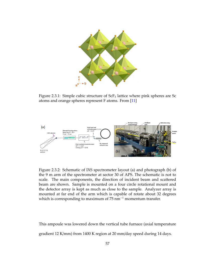
Figure 2.3.1: Simple cubic structure of ScF3 lattice where pink spheres are Scatoms and orange spheres represent F atoms. From [11]
Figure 2.3.2: Schematic of IXS spectrometer layout (a) and photograph (b) ofthe 9 m arm of the spectrometer at sector 30 of APS. The schematic is not toscale. The main components, the direction of incident beam and scatteredbeam are shown. Sample is mounted on a four circle rotational mount andthe detector array is kept as much as close to the sample. Analyzer array ismounted at far end of the arm which is capable of rotate about 32 degreeswhich is corresponding to maximum of 75 nm−1 momentum transfer.
This ampoule was lowered down the vertical tube furnace (axial temperature
gradient 12 K/mm) from 1400 K region at 20 mm/day speed during 14 days.
57

Figure 2.3.3: (a) Single crystal ScF3 received from Vladimir Voronov. We named
them for identification purpose in future usage. (b) Simple cubic structure
formation of ScF3 lattice drawn in to scale where purple spheres are Sc atoms
and red spheres represent F atoms.
The high momentum resolution (0.02 A−1), nine-analyzer collection scheme,
and microfocused x-ray beam permits measurements of the dynamical struc-
ture factor [101] within a transparent, isotropically pure, single-crystalline grain
[95, 96] of mosaic width 0.0020 (Figure 2.3.7(a)), as measured on the strong
(H,K,L) = (1,1,0) Bragg reflection indexed to the four-atom simple cubic cell
(Lattice parameter a = 4.016 A at temperature T = 300 K).
NTE in ScF3 was discovered only recently, and all most all the subsequent
reports on this effect have been reported in powder samples. We are only the
second single crystal of ScF3 investigators and first ever to carry IXS measure-
ments on ScF3. The IXS measurements were taken on crystal piece Gamma
58
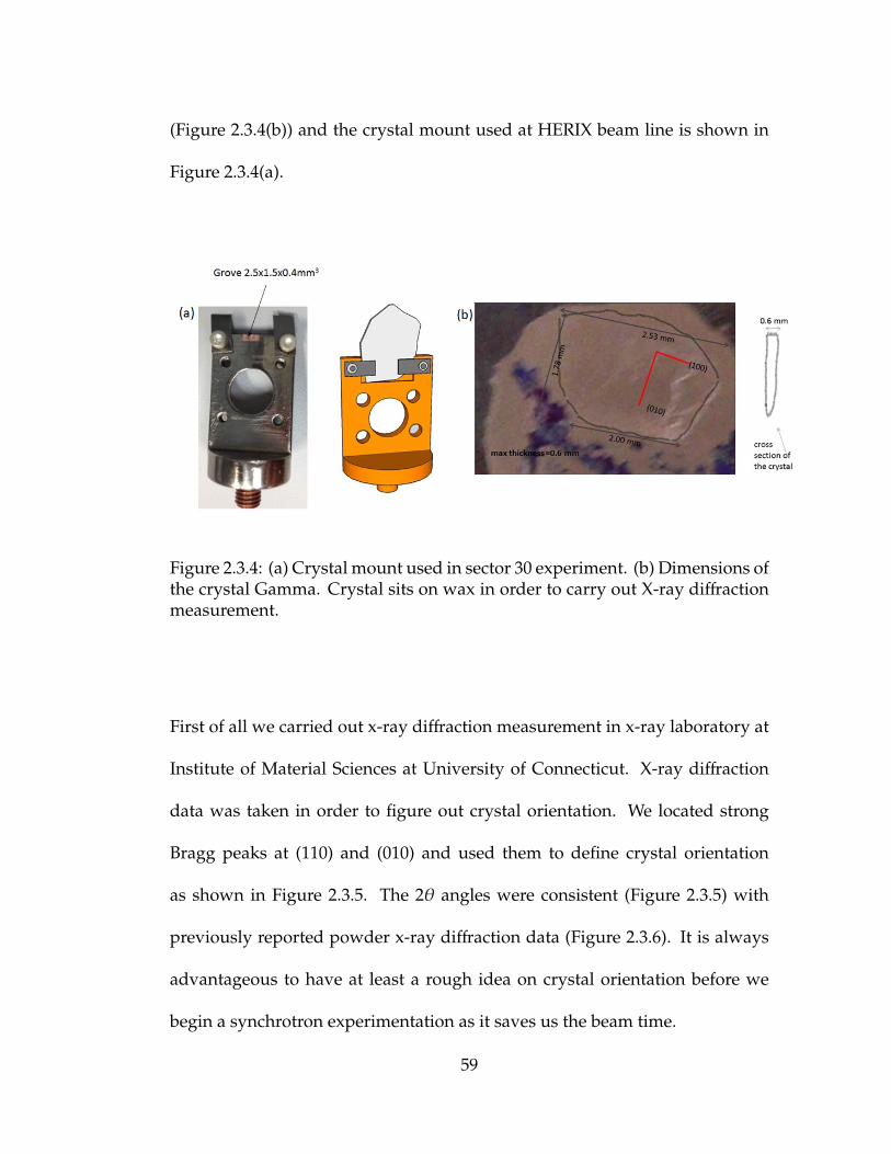
(Figure 2.3.4(b)) and the crystal mount used at HERIX beam line is shown in
Figure 2.3.4(a).
Figure 2.3.4: (a) Crystal mount used in sector 30 experiment. (b) Dimensions ofthe crystal Gamma. Crystal sits on wax in order to carry out X-ray diffractionmeasurement.
First of all we carried out x-ray diffraction measurement in x-ray laboratory at
Institute of Material Sciences at University of Connecticut. X-ray diffraction
data was taken in order to figure out crystal orientation. We located strong
Bragg peaks at (110) and (010) and used them to define crystal orientation
as shown in Figure 2.3.5. The 2θ angles were consistent (Figure 2.3.5) with
previously reported powder x-ray diffraction data (Figure 2.3.6). It is always
advantageous to have at least a rough idea on crystal orientation before we
begin a synchrotron experimentation as it saves us the beam time.
59

Figure 2.3.5: Diffraction spots appeared on 2D area detector. Crystal plane is
z=o and sample Gamma is used. Lattice planes are shown in dotted lines
Figure 2.3.6: X -ray diffraction data on powder ScF3 sample
60
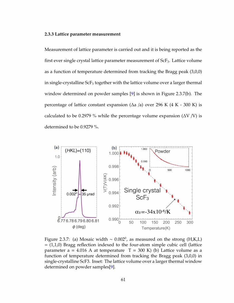
2.3.3 Lattice parameter measurement
Measurement of lattice parameter is carried out and it is being reported as the
first ever single crystal lattice parameter measurement of ScF3. Lattice volume
as a function of temperature determined from tracking the Bragg peak (3,0,0)
in single-crystalline ScF3 together with the lattice volume over a larger thermal
window determined on powder samples [9] is shown in Figure 2.3.7(b). The
percentage of lattice constant expansion (∆a /a) over 296 K (4 K - 300 K) is
calculated to be 0.2979 % while the percentage volume expansion (∆V /V) is
determined to be 0.9279 %.
Figure 2.3.7: (a) Mosaic width ∼ 0.0020, as measured on the strong (H,K,L)= (1,1,0) Bragg reflection indexed to the four-atom simple cubic cell (latticeparameter a = 4.016 A at temperature T = 300 K) (b) Lattice volume as afunction of temperature determined from tracking the Bragg peak (3,0,0) insingle-crystalline ScF3. Inset: The lattice volume over a larger thermal windowdetermined on powder samples[9].
61

2.3.4 Phonon dispersion relation
Dispersion through different cuts were investigated in reciprocal space at 300
K and 8 K and most interesting dispersion emerged along the M − R branch.
This is because the entire branch gets softer (∼ 3.5 meV at 300 K) with low
dispersion.
Figure 2.3.8: Overview of the lattice mode dispersion at select momenta andenergies. Strong branch softening along the M − R cut is shown by arrows.The longitudinal (LA) and transverse (TA) acoustic branches are shown. Blacksolid lines are a guide to the eye. Red circles in the inset mark the momenta R+ δ (2.39,1.43,0.45) and M + ε (2.39,1.43,0.02)
As explained earlier(section 2.2.1), we have measured a fundamental property
which contains information on the spatial and temporal fluctuation of the lattice
degree of freedom in ScF3. Figure 2.3.8 shows an overview of the lowest-energy
mode dispersion in ScF3 along high-symmetry directions determined by fitting
the structure factor to a damped harmonic oscillator model (Please refer section
2.3.14 for detailed explanation) along the cut from the Brillouin zone (BZ) face
62

center X to the BZ edge center M, an optic mode crosses the acoustic branches
and softens dramatically to a low energy of 3.5 meV at room temperature.
Cooling the sample to 8 K results in a dramatic and uniform softening of this
entire M−R branch to ∼ 1 meV, further suggesting an approach to a structural
instability near zero temperature.
2.3.5 M-R branch and NTE
The mechanism of ScF3 NTE behavior has been explained by the transverse
fluctuations of octahedra around the axis F-Sc-F of ScF6. Since these fluctuations
which support RUM, correspond to momentum at M and R points in the
reciprocal space which preserves the octrahedra integrity and do not involve
bond bending and stretching mode in the crystal, it appeared to be the most
interesting points to study. So we carried out the second phase of the IXS
measurement specifically at M and R points for 15 different temperatures down
to 3.8 K (Minimum we could achieve) and observed phenomenal physics. Other
than the phonon softening that we mostly expected we were able to observe
an elastic peak appearance as the temperature is lowered.
The low M−R branch is a near-degenerate manifold of cooperative vibrational
modes which are soft because they largely preserve the internal dimensions
of the stiff metal-anion molecular subunits. In order to retain local constraints
of bond distances and angles, staggered rotations induce a shrinking of the
cell dimensions, establishing a long-range coupling between local transverse
63

Figure 2.3.9: 〈100〉 planar section of the octahedra, illustrating the displacementpattern of modes attributed to NTE. The area of the box in (b) is reduced bycos2θ of the area in (a)
linkage fluctuations and lattice volume that has long been ascribed as the cause
of structural NTE.
2.3.6 M-R branch and phase transition
M−R is an important mode branch in perovskites because temperature-driven
condensation of modes on this branch can describe many structural transitions
which accompany ordering transitions of other types [84, 102, 103]. These
soft modes circumscribe the BZ edges (Figure 2.3.10) within a very narrow
window of energy set by the M − R branch dispersion, with the R point 200
µeV lower at all temperatures measured, consistent with an approach to the
symmetry-lowered rhombohedral R3c structure, as observed in other 3d BF3
systems.
The rhombohedral R3c structure is related to the high temperature cubic Pm3m
64

structure via a staggered octahedral tilt around the 〈111〉 axis, corresponding
to a frozen R+4 lattice distortion (Figure 2.3.11a). The staggered 〈111〉 octahe-
dral rotation angle is therefore the order parameter of the rhombohedral phase.
The free-energy curvature and origin of cubic-phase stabilization in trifluorides
has been addressed in a body of theoretical and computational work aimed to
generally understand perovskite structural phases. Density functional theory
[104], molecular dynamics [105], and exact electrostatic energy considerations
[106] of the insulating AlF3 prototype trifluoride suggest that Madelung en-
ergy including static electric dipole-dipole and induced dipoleinduced dipole
interactions compete to determine the stability of the cubic phase, and result
in a low-temperature rhombohedral phase.
Figure 2.3.10: First Brillouin zone of simple cubic material ScF3. High symmetry
points are shown as well.
65

It has been pointed out [106] that these competing influences could cancel
identically for larger metal radii, marginally stabilizing the cubic phase for all
temperatures, and it appears this limit is realized for ScF3. This suggestion
is supported by related previous work using momentum-integrated time-of-
flight neutron spectroscopy on bulk powder samples of ScF3 that showed a tem-
perature dependence of high-energy < 10 meV peaks in the neutron-weighted
density of states and included calculations suggesting the curvature of the R+4
mode is quartic in the tilt angle [68]. In what follows we present a momentum,
energy, and temperature-resolved investigation of the approach to the quan-
tum phase transition between the simple cubic and rhombohedral phases and
its effects on the lattice dynamics of perovskite ScF3.
Figure 2.3.11: (a) The lowest vibrational modes at the M point.(M+3 distortion)
(b) The lowest vibrational modes at the R point. The rhombohedral phase can
be described as a static tilt according to the R+4 pattern.
66

2.3.7 Central peak of ScF3
Background of central peak
An elastic peak was observed, accompanying with soft mode as SrTiO3 ap-
proaches structural phase transition and this was first discovered by Norwe-
gian physicist Tormod Riste in 1971[17]. Prior to this discovery he had worked
on magnetic systems and observed elastic-like peaks and soft modes associated
with spin diffusion on theses systems. While he was continuously working on
this, he was able to confirm the simultaneous existence of two modes such
as quasi-elastic peak(central peak) and soft mode near the critical region of a
phase transition in SrTiO3[12]. At the same time, he observed the central peak
dominates the scattering close to the transition temperature(Figure 2.3.12).
Gen Shirani was interested in this phenomenon and was able to carry an el-
egant experimental work at Brookhaven national lab using various samples.
Most of his interpretations came with the help of high-resolution spectra of
strain-free SrTiO3 samples[12]. By observing these spectra, two clear energy
scales associated with soft phonon energy and central peak linewidth were
identified. In other words, in addition to the relative short relaxation time
of the system characterizing the soft phonon, there exists a large relaxation
time characterizing the narrow central peak. Apart from that he clearly ob-
served the divergence of central peak as the transition temperature approaches
and confirmed that the structural phase transition deviated from mean field
67

theory like behavior. Since then the central peak has been observed as-
sociated with phase transition in many other perovskite structures such as
KMnF3[12], LaAlO3[107], RbCaF3[108], PbTiO3[109]. Central peak was also ob-
served in materials with vastly different properties like insulating Pb4Ge3O11,
NaNO3[110], KH2PO4[111], metallic ZrTe3[112], Ferroelastic LaAlO3[107], Fer-
roelectrics SrTiO3[17], Lead Germanate[113], KH2PO4[111], Ferromagnetic ma-
terial Rb2CrCl4[114], Antiferromagnetic materials YMnO3[115], CsCoBr3[116],
Superconductors BSCCO[117], YBa2Cu3O6.6[118], Nb3Sn[119].
Figure 2.3.12: (a) Inelastic spectra of SrTiO3 measured at several temperatures.
Left side shows the soft mode behavior and right side shows divergence of
central peak. From [12]. (b) Inelastic spectra of SrTiO3 (left) and KMnF3 (right)
for approximately equal ∆T=T-Tc. From [12].
2.3.8 What causes central peak?
Though central peaks have been observed in nearly all systems exhibiting struc-
tural phase transitions, their origins are still under debate[120]. While one class
68

of theories has proposed that the central peak is the result of intrinsic nonlin-
ear mechanisms such as the presence of solitons[121], another class of theories
suggests that it is an extrinsic effect due to defects[120]. At the beginning,
there were theoretical grounds for believing in the existence of the central peak
in three dimensions as well as lower dimensional systems [121, 122]. Mecha-
nisms related to defects have been proposed and are based on the observations
that the central peak is sample dependent[123]. In a ferroelectric material, the
central peak can even be made to disappear by annealing the sample[124]. In
the defect mechanism, the central peak is associated with the local distortion
of the atoms about the defect[125, 119]. This displacement field gives rise to
diffuse scattering of x-rays or neutrons and is usually referred to as Huang
scattering. Even though the Huang scattering is usually observed near Bragg
peaks, enhanced scattering at ω0 = 0 may still appear in the presence of soft
modes at the soft mode q-vector. In this case, the soft mode should be coupled
with impurities and further evidence for this extrinsic effect came through an
experiment[13] on SrTiO3(Figure 2.3.13). There the central peak intensity was
enhanced with an increase in defect concentration but the exact relationship
was found to be not proportional. Further, the exact dependency was difficult
to compare among different impurity systems as well[14]
69

Figure 2.3.13: Central peak due to defects and impurities. (a) Integrated central
peak intensity of hydrogen reduced SrTiO3 as a funtion of T-Tc [13]. (b) The
temperature dependence of the central peak height of the as-grown KH3(SeO3)2
crystal (+) and the crystals used repeatedly (0, ,x)[14]
High momentum resolution x-ray data near phase transition temperature could
be decomposed into a sharper peak and a broader peak which proposed two
length scales associated with the dynamics of both soft mode and the central
peak. Even though the origin of these peaks was debatable, the scattering
intensities measured by probing the surface and the bulk of the same sample
separately supported the fact that the sharp component is not an intrinsic
property but related to the difference between the bulk and the outer surface
of the sample.
70

Figure 2.3.14: Broad and narrow features within the central peak. Solid and
dotted curves in (a) represent fitting models, Lorenzian squared and Lorenzian
function respectively[15]. (b) X-ray scans of12
(1,1,5) R point along [0 1 1]
direction with 100 keV photon energy beam hitting at the center of the crystal
and (c) beam hitting the crystal corner of the crystal. )[16]
Other than the extrinsic effects such as impurities and defects the appearance of
the central peak can be sorted out due to intrinsic behaviors such as fluctuations
due to phonon density, solitons, nonlinear effects etc. Central peak originated
from intrinsic mechanisms was reported in NaNO3 due to the mobility of
NO−3 ions as it approaches order-disorder phase transitions[110]. Theoretical
work by Krumhansal and Schrieffer suggested that the domain walls or cluster
boundaries between large ordered regions in the crystal may cause central peak
as well[126, 127]. In LaAlO3 the central peak mode(s) has been interpreted in
terms of phonon density fluctuations and flipping of clusters of tilted octahedra
71

between different orientations[128].
2.3.9 Central peak of ScF3 and mode softening
Figure 2.3.15 shows the temperature-dependent IXS spectra for ScF3 at M(2.5,1.5,0)
and R(2.5,1.5,0.5) points, where the dynamical structure factor is particularly
strong for the modes of Figures 2.3.11a and 2.3.11b. Clear soft mode behavior
is observed concomitant with the emergence of a strong elastic peak, which
onsets at ∼ 80 K and strengthens dramatically as the temperature is lowered.
The elastic peak emergence is also observed at momenta away from the high-
symmetry M-R cut from data collected in an adjacent analyzer channel. Figure
2.3.16 shows IXS data at M + ε (2.39,1.43,0.02) and R + δ (2.39,1.43,0.45) momen-
tum points, where the optical branch is much stiffer (56 meV) and displays a
milder degree of softening, making the distinction between the elastic peak and
soft mode phenomena more apparent in the raw data. In all cases, a transfer
of spectralweight from the optical mode to the central peak feature is observed
as the temperature is lowered.
All data were fit using a resolution-convoluted model for the dynamical struc-
ture factor,which includes a damped harmonic oscillator and a detailed balance
condition to describe the lattice mode, and a resolution-limited elastic central
peak, consistent with previous analyses of this phenomena in SrTiO3 and other
materials [12] (see section 2.3.14). This analysis allows us to extract the soft
mode frequency and strength A0 of the central peak. Figure 2.3.17 shows that
72

Figure 2.3.15: Color maps of the IXS signal at the (a) M (b) R points in reciprocalspace
Figure 2.3.16: Color maps of the IXS signal at the (c) M +ε, and (d) R + δ pointsin reciprocal space.
the temperature dependence of the lowest soft mode frequency behaves ap-
proximately as ω2∝ (T − Tc) as expected from classical mean-field theories
73

of structural phase transitions [120]. This simple extrapolation of the R point
soft mode frequency suggests that the phase transition occurs at Tc ∼ -39 K,
so it does not occur for any finite temperature, consistent with observations
[9, 20, 19, 97]
Figure 2.3.17: Resolution convoluted fitting of the IXS data in figure 2.3.16results in squared mode energies
Central peaks and mode softenings observed in the context of the 110 K cubic-
to-tetragonal transition of incipient ferroelectric SrTiO3 [12, 17, 129, 130] ,are
commonly associated with an approach to a structural phase transition. There,
the elastic central peak has maximum strength at Tc but begins to appear
up to 25 K higher [12, 130]. In the present case, we observe(Figure 2.3.19)
no maximum in elastic scattering at any finite temperature and the intensity
continues to strengthen at the lowest temperatures measured (3.8 K). In ScF3,
the effect of the central peak begins above 80 K, suggesting that precursor
74

Figure 2.3.18: Resolution convoluted fitting of the IXS data in figure 2.3.16results in elastic peak intensity. Elastic peak begins to appear near 80 K, whichis 120 K above the extrapolated transition temperature.
Figure 2.3.19: Central peak intensity observed in SrTiO3 [17]. Elastic peak be-gins to appear 25 K above the transition and the intensity reaches it’s maximumat the transition temperature.
effects occur as high as 120 K above our extrapolated transition temperature.
The thermally robust central peak in ScF3 occurs in our strain-free, (naturally)
isotopically pure, color center-free single crystalswith a narrow(0.002)mosaic.
Interestingly, the elastic peak begins to strengthen at the same temperature scale
75
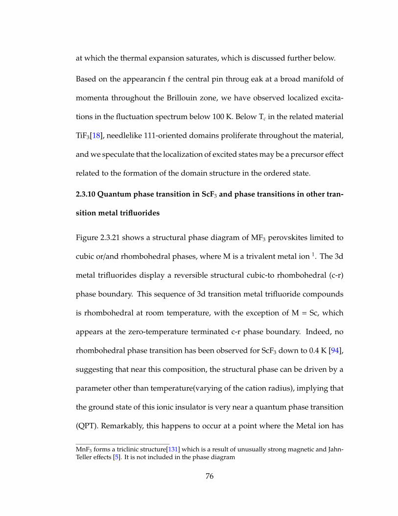
at which the thermal expansion saturates, which is discussed further below.
Based on the appearancin f the central pin throug eak at a broad manifold of
momenta throughout the Brillouin zone, we have observed localized excita-
tions in the fluctuation spectrum below 100 K. Below Tc in the related material
TiF3[18], needlelike 111-oriented domains proliferate throughout the material,
and we speculate that the localization of excited states may be a precursor effect
related to the formation of the domain structure in the ordered state.
2.3.10 Quantum phase transition in ScF3 and phase transitions in other tran-
sition metal trifluorides
Figure 2.3.21 shows a structural phase diagram of MF3 perovskites limited to
cubic or/and rhombohedral phases, where M is a trivalent metal ion 1. The 3d
metal trifluorides display a reversible structural cubic-to rhombohedral (c-r)
phase boundary. This sequence of 3d transition metal trifluoride compounds
is rhombohedral at room temperature, with the exception of M = Sc, which
appears at the zero-temperature terminated c-r phase boundary. Indeed, no
rhombohedral phase transition has been observed for ScF3 down to 0.4 K [94],
suggesting that near this composition, the structural phase can be driven by a
parameter other than temperature(varying of the cation radius), implying that
the ground state of this ionic insulator is very near a quantum phase transition
(QPT). Remarkably, this happens to occur at a point where the Metal ion has
MnF3 forms a triclinic structure[131] which is a result of unusually strong magnetic and Jahn-Teller effects [5]. It is not included in the phase diagram
76

stoichiometric occupation with a full electronic shell, permitting a clean study
of fluctuating quantum matter from structural degrees of freedom without also
having to consider additional electronic and magnetic degrees of freedom. The
phase boundary is most likely continuous, considering the observation that
the c-r transition in TiF3 appears to be second order[132]. Cubic ScF3 further
stands out among substances in that it has the most stable structural phase of
any known solid trifluoride[23].
Figure 2.3.20: Cubic and rhombahedral unit cells associated with two phasesof transition metal trifluorides other than ScF3 are shown. As shown therhombahedral phase is associated with rotated ScF6 sub units. Gray circlesrepresent scandium atoms and light blue circles represent fluorine atoms.
The c-r structural transition can be stabilized at finite temperature through sub-
stitution of other metals (Al, Ti, Y) for Sc, or in pure ScF3 through application
of very low hydrostatic pressures [95, 95] (> 0.2 GPa) at cryogenic tempera-
tures. Remarkably, using the observed pressure dependence of the transition
temperature dTc/dp ∼ 525 K/GPa [9, 95, 96], and the putative transition tem-
77

perature Tc∼ -39 K, one can estimate that pressures as small as 740 bar = 0.074
GPa would be sufficient to drive the transition upward to 0 K, permitting a
clean manner in which to observe a structural quantum phase transition. The
sensitivity of the phase boundary to these external changes suggests that the
nature of the cubic phase is delicate at low temperature and susceptible to even
mild perturbations. Chemical substitutions of Sc by Ti [20], Al [19], and Y [97]
have been reported and Tc is presented in Figure 2.3.21. The phase boundary
in Sc1−xTixF3 appears to linearly interpolate between the end members ScF3 and
TiF3 with no maxima or minima at intermediate compositions, consistent with
a picture where the substitution of wellmatched ionic radii (rTi = 0.670 A ; rSc =
0.745 A ) uniformly affects the potential landscape and gradually changes the
phase stability.
2.3.11 ScF3 systems and disorder
On the other hand, substitution of ions with radii much smaller (rAl = 0.535
A ) or much larger (rY = 0.90 A ) than Sc stabilizes the rhombohedral phase,
suggesting the role of disorder is strong for these substitutions. We quantify
the disorder in these solid solutions by using the variance of the B-site ion
distribution σ2B = 〈 rB - 〈rB〉 〉
2 as determined from the nominal chemical formula
in these solid solutions,and plot the disorder phase diagram in Figure 2.3.22.
The trend in Tc(σ2B) is an example of the general case, wherein electronic (su-
perconducting, magnetic) and structural (ferroelectric, ferroelastic) transitions
78

Figure 2.3.21: Structural phase diagram showing the c-r phase boundary vs theB-site mean radius in 3d transition metal trifluorides and in the solid solutionsSc1xAlxF3 and Sc1xYxF3. Data taken from Refs [18, 19, 20, 21, 22].
have opposite sensitivities to disorder, as determined through studies of the
A-site variance effect on phase stability [133, 134]. The latter case, relevant
here, occurs because local strain associated with substitution has the effect
of disrupting long-range propagation of strain, enhancing the stability of the
lowered-symmetry phase. Generalizing these trends to B-site disorder near the
composition ScF3, we separately fit the transition temperatures Tc(x) = T0c−p1σ2
B
to the doped compositions of Al and Y substitution and find that extrapolat-
ing transition temperatures of the doped compositions to the ideal case σ2B = 0
79

gives roughly similar T0c= 75 K (Al) and 104 K (Y), which is near the temperature
scale where we observe a strong elastic peak emergence (Figure 2.3.19) and the
thermal expansion coefficient departs from linear dependence on temperature
(Figure 2.3.7). Empirically, Tc > 0.4 K is observed for pure ScF3, suggesting
a strong deviation from previous studies [133, 134] and qualitatively different
physics in the pure limit.
80

Figure 2.3.22: Disorder phase diagram for ScF3. Compositional disorder is
quantified via the B-site variance σ2B = 〈 rB - 〈rB〉 〉
2, which has the effect of
increasing the stability of the lowersymmetry, rhombohedral structural phase.
Red and orange symbols show the effect of Y and Al substitution, respectively.
Dotted lines indicate a linear fit to the Tc(σ2B), not including the pure sample ScF3.
The vertical axis intercept reveals a temperature scale ∼ 80-100 K,where central
peak elastic scattering and thermal expansion saturation are also observed in
pure ScF3
2.3.12 Transverse motion of F atoms
The ScF6 octahedra in pure ScF3 move collectively in a state of strong orien-
tational fluctuation [106, 135], the strength of which can be estimated from
81

powder refinement of the anisotropic thermal parameter U33, associated with
transverse F motion. The orientational fluctuations are significant [9], ap-
proaching 2√
U33/a ∼ 9.2 full width at half maximum (FWHM) at room tem-
perature, significantly larger than the isostructural oxide ReO3 [133].
Figure 2.3.23: Transverse vibrations of Fluorine atom
In this regime, the influence of long-ranged strain draws in the lattice, leading
to a robust and sizable NTE effect. At elevated temperatures, long-range strain
fields imposed by local constraints propagate over much shorter distances,
and the fluctuation spectrum lacks a central peak and appears more conven-
tional. The long-range strain effects we have observed are likely present in the
physics of structural transitions in perovskite and other structural classes, but
are particularly enhanced in ScF3 at low temperature.
2.3.13 Elastic parameters of ScF3
The combined energy (1.5 meV) and momentum (0.2 nm−1) resolution allowed
us to observe the phonon branches extending over the entire lattice spectral
bandwidth of 85 meV. We have made special efforts and acquired IXS spectra
relevant to the acoustic modes along [110] and [100]. The acoustic mode ener-
82

gies were plotted against several reduced momenta near (300) and (220) in the
brillouin zone as shown in Figure 2.3.24.
Figure 2.3.24: Acoustic phonon energies along different directions in reciprocalspace. The slope simply gives the acoustic velocities of corresponding modesalong different directions for ScF3. LA and TA stands for longitudinal acousticsand transverse acoustics respectively
vp[100] = (c11/ρ)1/2 (2.3.1)
vs[100] = (c44/ρ)1/2 (2.3.2)
vp[110] = (c11 + c12 + 2c44/2ρ)1/2 (2.3.3)
vs[110] = (c11 − c12/2ρ)1/2 (2.3.4)
83

Where ρ is the density of the sample. vp and vs are longitudinal and trans-
verse acoustic wave velocities respectively which are defined along both the
principle axis [100] and [110]. Data were fit to determine the transverse and
longitudinal sound speeds separately as summarized in Figure 2.3.24. The
value obtained for vs[100] is 2871.7 ms−1. vp[100] and vp[110] are 7809.3 ms−1
and 7118.1 ms−1 respectively. Given the density of ScF3 is 2.53 g/cm3 and using
Equations 2.3.2 - 2.3.5 the elastic parameters C11, C12, and C44 are determined.
Using elastic parameters the bulk modulus(B) and the shear modulus(G) of the
crystal were calculated. The corresponding relationships for cubic symmetry
are elaborated in section 7.2.1 in Chapter 7. Our values from IXS measure-
ments are summarized in Table 2.3.2 and compared with previously estimated
values based on calculations[96, 94] for ScF3 and previously estimated values
based on measurements for ZrW2O8 [136] and for ReO3[137]. Figure 2.3.25 and
2.3.26 show some of the elastic properties derived from the measured elastic
constants.
Material C11 (GPa) C12 (GPa) C44 (GPa) B (GPa) G (GPa) A (GPa)——————————–————–————–————-———–————-ScF3 (ours) 161.4 63.13 21.8 95.88 32.73 0.44ScF3 [96] 172.7 18.9 18.6 70.2 41.92 0.24ScF3[94] 230 17.3 18.0 88.2 53.34 0.17ZWO [136] 128.4 47.5 27.4 74.5 433.9 0.68ReO3[137] 717 71.1 103 286 190.98 0.32
Table 2.3.2: Summary of elastic properties of similar type of materials. Bulkmodulus (B), Shear modulus (G) and Zener anisotropy (A) are shown as well
Experimentally determined coefficients C11 and C44 are very much agree with
84

calculated values but C12 is off by 45 GPa. It is clear from the equation 2.3.3 that
C12 is related to transverse acoustic phonon along [110] direction. Therefore
the difference is obviously related to corresponding phonon energies measured
using IXS. One could argue that transverse acoustic phonons along [110] should
be stiffer than along [100] which results in decrease in C12. On the other hand
the zener anisotropy value estimated from our measurements is close to 1
compared with the theoretical zener anisotropy value. As a result, we argue
that our measurements interpret the isotropic nature of the single crystal ScF3
more accurately than calculations.
Figure 2.3.25: Poisson ratio obtained from elastic parameters
85
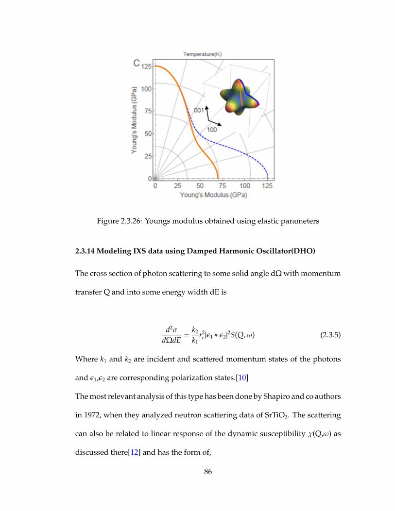
Figure 2.3.26: Youngs modulus obtained using elastic parameters
2.3.14 Modeling IXS data using Damped Harmonic Oscillator(DHO)
The cross section of photon scattering to some solid angle dΩ with momentum
transfer Q and into some energy width dE is
d2σdΩdE
=k2
k1r2
e |ε1 ∗ ε2|2S(Q, ω) (2.3.5)
Where k1 and k2 are incident and scattered momentum states of the photons
and ε1,ε2 are corresponding polarization states.[10]
The most relevant analysis of this type has been done by Shapiro and co authors
in 1972, when they analyzed neutron scattering data of SrTiO3. The scattering
can also be related to linear response of the dynamic susceptibility χ(Q,ω) as
discussed there[12] and has the form of,
86

S(Q, ω) =1π
11 − exp−βω
Im[χ(Q, ω)] (2.3.6)
The damped harmonic oscillator(DHO) response used to describe phonons in
solid is,
χ(Q, ω)−1 = ω∞(Q)2− ω2
− iωΓ(ω) (2.3.7)
most importantly with a frequency dependent damping constant
Γ(ω) = Γ0 +δ2
γ − iω(2.3.8)
Here the additional frequency dependent damping represents another decay
channel with relaxation time of 1/γ and coupling strength of δ. Combining
Equations 2.3.6,2.3.7 and 2.3.8 Shapiro separated the dynamic structure factor
into two components, central peak and soft phonon mode.
Since the energy resolution is limited in IXS measurements, we avoided using
the same DHO function. Instead we chose a DHO with a constant damping
constant(Γ0) and a resolution limited Lorentzian(L) as our model to fit the
experimental data. The model was convoluted with the resolution function and
then was evaluated at each data point. The width (wL) of the resolution limited
Lorentzian and the center frequency (ω0) were fixed to 0.1 and 0 respectively,
while the amplitude (A0) was kept as a free parameter. All fit parameters of
DHO were set free except the sample temperature, which (T) was fixed to the
87

measured value.
Fit parameters used can be identified as, A - the amplitude of the DHO, ω∞ -
the center frequency of the DHO, A0 - the amplitude of the Lorentzian and Γ0 -
the full width half max of the DHO.
The Lorentzian is defined as:
L(ω,wL, ω0,A0) =A0wL
2π1
(ω − ω0)2 + (wL
2)2
(2.3.9)
Figure 2.3.27: Representative resolution function collected at 6K from plexiglassco-mounted with the sample
The DHO is given by:
DHO(ω,ω∞,T,Γ0,A) =A
(1 − exp−ω/T)πωΓ0
(ω2∞ − ω2)2 + (ωΓ0)2
(2.3.10)
The resolution function at each temperature was experimentally determined by
88
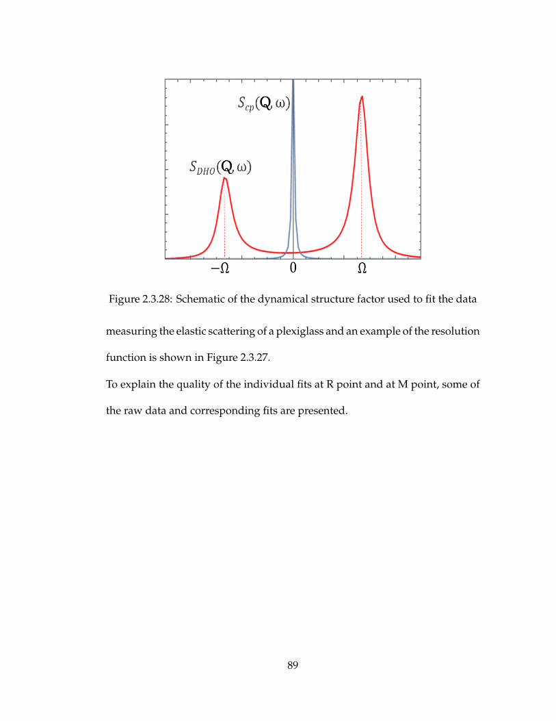
Figure 2.3.28: Schematic of the dynamical structure factor used to fit the data
measuring the elastic scattering of a plexiglass and an example of the resolution
function is shown in Figure 2.3.27.
To explain the quality of the individual fits at R point and at M point, some of
the raw data and corresponding fits are presented.
89

Figure 2.3.29: Sample of fit quality at momentum points R (left column) andM (right column). The red points and blue lines resemble data and the fitrespectively.
90

Figure 2.3.30: Sample of fit quality at momentum points R+δ (left column) andM + ε (right column).
91

Chapter 3
Comparative study of two incipient ferroelastics,ScF3 and Hg2I2
3.1 Introduction
As introduced in Chapter 1, ScF3 is a prominent SNTE system forming in
the so called ”open” perovskite structure. Recent work [28] has described the
configurational potential for R point distortions as having a nearly quartic form
at small displacement, presenting an interesting limit of lattice dynamics.
Inelastic investigations discussed in Chapter 2 on single crystals show a soft-
mode instability and other phenomena that indicate a structural transition
with extrapolated critical temperature Tc < 0, meaning that while similar com-
pounds like TiF3 realize a cubic-to-rhombohedral structural phase transition,
this transition is never realized in ScF3, except under an extremely small < 1
kbar hydrostatic pressure at cryogenic temperatures. These special circum-
stances are contextualized in Figure 3.2.1a, which shows the global structural
phase diagram of 3d transition metal trifluorides BF3 as a function of the B+3
ionic radius, rB. The occurrence of the endpoint of a structural phase boundary
so near the ground state of a stoichiometric compound is extremely rare, as
92
is the pronounced SNTE property of ScF3. The confluence of these unusual
circumstances raises the question of whether certain types of NTE can arise
as unusual behavior above structural quantum phase transitions (SQPTs) due
in this case to strong geometrical fluctuations of the incipient ferroelastic state
(IFE) occuring either through quantum effects, or classical energy landscape
flattening. To directly address this issue, we have explored the thermal expan-
sion behavior and lattice fluctuation spectra in optical/detector quality single
crystals of a second stoichiometric IFE in mercurous iodide, Hg2I2, known
colloquially as protiodide [138].
We note that incipient lattice instabilities have recently attracted renewed inter-
est [139] in light of their use to develop a 50% increase [140] in superconducting
transition temperature of Nb-doped SrTiO3 in an exceptional limit of the strong
coupling theory [141], while the recent observation of electronic coupling to
a substrate phonon in FeSe films raises questions regarding the possible role
of substrate lattice fluctuations in stabilizing film superconductivity[142]. The
common appearance of incipient soft modes also in SNTE materials potentially
opens promising areas for future work combining SNTE and superconductivity
to realize new emergent phases enabled by extremal strain conditions. Previous
evidence from our study of ScF3[23] and other systems [134] has determined
that quenched disorder can have dramatic effects on structural instabilities,
and we have restricted our attention to pure stoichiometric systems, in contrast
to a recent study of a SQPT achieved through chemical substitution, showing
93
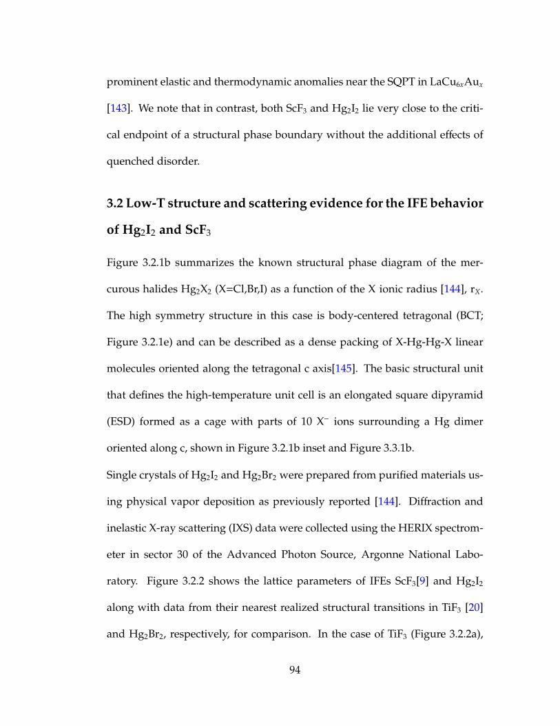
prominent elastic and thermodynamic anomalies near the SQPT in LaCu6xAux
[143]. We note that in contrast, both ScF3 and Hg2I2 lie very close to the criti-
cal endpoint of a structural phase boundary without the additional effects of
quenched disorder.
3.2 Low-T structure and scattering evidence for the IFE behavior
of Hg2I2 and ScF3
Figure 3.2.1b summarizes the known structural phase diagram of the mer-
curous halides Hg2X2 (X=Cl,Br,I) as a function of the X ionic radius [144], rX.
The high symmetry structure in this case is body-centered tetragonal (BCT;
Figure 3.2.1e) and can be described as a dense packing of X-Hg-Hg-X linear
molecules oriented along the tetragonal c axis[145]. The basic structural unit
that defines the high-temperature unit cell is an elongated square dipyramid
(ESD) formed as a cage with parts of 10 X− ions surrounding a Hg dimer
oriented along c, shown in Figure 3.2.1b inset and Figure 3.3.1b.
Single crystals of Hg2I2 and Hg2Br2 were prepared from purified materials us-
ing physical vapor deposition as previously reported [144]. Diffraction and
inelastic X-ray scattering (IXS) data were collected using the HERIX spectrom-
eter in sector 30 of the Advanced Photon Source, Argonne National Labo-
ratory. Figure 3.2.2 shows the lattice parameters of IFEs ScF3[9] and Hg2I2
along with data from their nearest realized structural transitions in TiF3 [20]
and Hg2Br2, respectively, for comparison. In the case of TiF3 (Figure 3.2.2a),
94

Figure 3.2.1: Structural phase diagrams of (a) 3d transition metal trifluoridesand (b) mercurous halides. Insets show the basic volume-defining polyhedralunits: (a) the BF6 octahedraon and (b) the elongated square dipyramid (ESD).Development of the structure for (c) the trifluorides and (d) the mercuroushalides with the ionic radii indicated as spheres. The basic polyhedral structuralunit is superposed in each case. (e) Comparison of the observed bond distances(symbols) and expectations based on hard sphere packing (dashed lines).
95

Figure 3.2.2: Temperature-dependent lattice parameters of (a,c) ScF3, TiF3, and(b,d,f) Hg2I2, and Hg2Br2. (e) shows a schematic free energy landscape ofrealized and incipient ferroelastics. Arrows show the fluctuation domain ineach case.
96

Figure 3.2.3: Rocking curves measured at (330) bragg peak for optical anddetector quality Hg2Br2 and Hg2I2 crystals cleaved along 〈110〉 planes grownby physical vapor deposition method by Brimrose Technology Cooperation.
the cubic-torhombohedral transition has profound effects on the lattice dimen-
sions, showing a signature step of first order transition and subsequent con-
tinuous order parameter development, shrinking ∼ 3% between the structural
transition temperature Tc and base temperature [19]. The hexagonal c axis
on the other hand displays SNTE similar in magnitude to the negative CTE
observed in ScF3 in the same temperature range. The lattice expansion of the
realized transition in Hg2Br2 bears remarkable resemblance, with a significant
reduction in tetragonal c axis lattice parameter below the transition, changing
4.5% between 150K and base temperature. The transition appears to be nearly
continuous, consistent with prior work [146].
The c axis of Hg2I2 however shows a clearly negative CTE below 100K shown in
Figure 3.2.2d, reaching a significant low-temperature value of -5ppm/K. While
negative values of the c-axis compressibility have been noted in mercurous
halides [147], SNTE in Hg2I2 has not been reported to our knowledge. The
97

similarities to the fluorides are striking - both realized transitions TiF3 and
Hg2Br2 show strong positive CTE below their respective transitions while the
IFE systems tuned near their SQPTs show strengthening NTE at the lowest
temperatures. The magnitude of the negative CTE in the iodide case (-5ppm/K)
is about one third of the maximum magnitude in the trifluoride case (-14ppm/K)
and the range of thermal persistence is also reduced about 10-fold. These
reductions can be partially explained by the large mass difference between the
two materials classes and the correspondingly different energy scale of thermal
fluctuations required to induce bond-stretch fluctuations, whose presence may
mute the long-range effects coupling bond-bend modes to lattice dimensions.
We remark that at the outset the geometrical similarities in the structure of
these two classes and explore more detailed analysis of the influences driving
these incipient structural transitions in each case below
3.3 Discussion and SNTE material design principles
The halide ESD is not regular, but rather compressed, defined by X-X bond
lengths of three varieties: the long X-X bonds (green) lying in the basal plane,
the short X-X bonds (blue) oriented along the tetragonal c axis, and apical X-X
bonds (red). Figure 3.2.1d shows reported literature values of the lengths of the
three types of X-X bond distance [145, 148, 149, 138, 150, 151]. The basal planar
(green) X-X bonds cluster well 2 with a clear trend far in excess of the diagonal
The clustering for the X-X (a) bonds is due to the simple relation to structure - this bond distanceis simply the a lattice parameter and can be determined from a single reflection and Braggs
98

dashed line that indicates simplest expectation based on sphere packing. The
apical (red) bonds trend with ionic radius and stay near the X ionic diameter,
indicating the apical half octahedron is somewhat flattened relative to a regular
ESD, but roughly satisfies the simple packing conditions. On the contrary, the
coriented (blue) X-X bond is near the ionic diameter only for X=Cl (calomel)
and deviates significantly for X=Br and even more so for the IFE X=I, implying
these short bonds along c are in a state of compression due to forces provided
by the rest of the framework3. The natural source of this compression is a net
tension in the X-Hg-Hg-X linear molecule along the c axis through the ESD
center.
Starting from the BCT phase, the relevant distortion to the low-temperature
orthorhombic phase is a staggered shift of the Hg-Hg dimer from the ESD
central axis in the 110 direction of the basal plane (Figure 3.2.1f). The structural
transition then corresponds to condensation of the transverse acoustic wave at
the X point of the BCT Brillouin zone (shown in Figure 3.3.2b inset) [146, 153].
For these realized improper [146, 154] ferroelastic materials, Tc > 0 and the
T = 0 energy landscape consists of four minima corresponding to the possi-
ble saturated shifts of the Hg dimers (Figure 3.2.1b). For larger ionic radius,
these minima flatten and coalesce to the central axis for X=I and no symme-
law. The distances for the trifluoride show little scatter for the same reasons. The other internaldistances require refinement of many allowed Bragg reflections over a larger angular range soshow more scatter between reportsThis distance is much shorter than typical X-X distances obtained through searches of theinternational crystal database [152]
99

Figure 3.3.1: Structure of 3d transition metal trifluorides in the (a) high-temperature cubic phase and (b) the low-temperature rhombohedral phase.Structure of the mercurous halides in (c) the high-temperature body-centeredtetragonal and (d) low-temperature orthorhombic phases. Inelastic X-rays scat-tering measurement of (e) ScF3 at the simple-cubic R point, corresponding tothe soft mode of the rhombohedral transition and (f) Hg2I2 at the BCT X point,corresponding to the soft mode of the orthorhombic transition. Insets showthe Brillouin zone in each case. Soft mode frequency squared resultant fromfitting to a damped-harmonic oscillator model for (g) ScF3 at R point and (h)Hg2I2 at X point. Dashed lines indicate the extrapolation to negative absolutetemperature and indicate the proximity to an incipient ferroelastic transition.
100

try breaking is observed. The flattening of the energetic landscape however
induces strong temperature-dependent fluctuations of the staggered shift, as
is observed experimentally from X-ray diffraction data as large transverse di-
mensions of the Hg thermal ellipsoids, approaching 2√
U11 = 0.38 Å at T = 150
K for Hg2I2 [151]. We propose that the origin of the coalescing minima can
be viewed as an effect of two competing forces: the compressive stress on the
c-oriented XX bonds and the tensile stress on the X-Hg-Hg-X linear molecule
by its environment. For X=I, these forces have a near-canceling effect which
stabilizes the high-symmetry BCT structure and stabilizes transverse dimer
fluctuations inside the ESD.
In the language of structural mechanics, the development of a state of self
stress (SSS) in the ESD polyhedral unit [155] increases its tensile integrity (aka
tensegrity [156]). As is known in structural mechanics of frameworks, the
development of a SSS is accompanied by reduction of the zero mode count
[155, 157, 158], and the transition may be regarded as a reduction of this off-
axis degree of freedom.
The critically-tensioned linear molecule inside the ESD unit exhibits large trans-
verse fluctuations of the Hg dimer and leads to the observed negative thermal
expansion along this axis (Figure 3.2.1d). This size-induced stiffening is also
apparent in the lowering of the melting temperature and triple points as the
X ion grows, since the entropy of the BCT phase is reduced by the stiffening
of the ESD. To elucidate the connection between the unusual lattice parameter
101

behavior in scandium trifluoride and protiodide, we consider evolution of the
basic trifluoride octahedral subunit with rB, used as a baseline for comparison
of relative size effects. Figure 3.3.1c shows that to a good approximation, the
unit cell dimension F-B-F ionic distance (a lattice parameter) trends with rF +rB
while the nearest F-F distance grows to values significantly in excess of the
2rF . We note further that for rB > 0.75 Å in the rare-earth class and beyond,
trifluorides take on other crystal structures with B site coordination larger than
n=6 in the orthorhombic tysonite (n=8), and hexagonal (n=9) [159] structures.
Together, these observations suggest an effective reduction of the overall stiff-
ness of the BF6 octahedron for large B ions through reduced interaction of the
anions situated at the octahedral vertices. In this case, a large number of SSSs
are removed as the octahedral unit loses tensegrity with increasing rB. No-
tably, fluctuations of the F position transverse to the B-F-B bond are very large
in ScF3, approaching 2√
U33 = 0.24 Å [135, 160, 161] at T =150 K, consistent with
this picture. In contrast to the mechanism in the mercurous iodide, we expect
that the onset of pliancy of octahedral molecules stabilizes the cubic phase,
as many states are available with the average cubic structure. This situation
is also manifest in the high melting point of ScF3, where the high entropy of
transverse bond fluctuation competes with the fluid phase up to 1800 K.
Figure 3.2.1a,b show inelastic X-ray scattering spectra at the momentum points
corresponding to the soft mode instabilities in IFEs ScF3 and Hg2I2. The triflu-
oride lowtemperature phase can be described as a staggered tilt of ocathedra
102

Figure 3.3.2: Structure of 3d transition metal trifluorides in the (a) high-temperature cubic phase and (b) the low-temperature rhombohedral phase.Structure of the mercurous halides in (c) the high-temperature body-centeredtetragonal and (d) low-temperature orthorhombic phases. Inelastic X-rays scat-tering measurement of (e) ScF3 at the simple-cubic R point, corresponding tothe soft mode of the rhombohedral transition and (f) Hg2I2 at the BCT X point,corresponding to the soft mode of the orthorhombic transition. Insets showthe Brillouin zone in each case. Soft mode frequency squared resultant fromfitting to a damped-harmonic oscillator model for (g) ScF3 at R point and (h)Hg2I2 at X point. Dashed lines indicate the extrapolation to negative absolutetemperature and indicate the proximity to an incipient ferroelastic transition.
103

around the 111 axis (Figure 3.2.1f). This fluctuation has the (π, π, π) spatial
texture of the R point in the simple cubic Brillouin zone, shown in Figure 4a.
Also shown is a surface plot of the dynamical structure factor S(R,ω) obtained
using IXS [23]. At high temperature, a Stokes and anti-Stokes mode at low
frequency of 3.4 meV softens considerably, approaching an extrapolated tran-
sition temperature Tc' -39 K, as shown in Figure 3.2.1c. This singular point in
the response function is suggestive of a flattening of the free energy landscape
in an approach to an unrealized structural phase transition and strongly sup-
ports our identification of ScF3 as an IFE. Similarly, Figure 3.2.1b,d show the
evolution of S(X,ω) with temperature and an avoided condensation of a soft
mode at the X point of the body-centered tetragonal Brillouin zone in Hg2I2.
S(X,ω) again shows Stokes/anti-Stokes mode pairs that imply a putative tran-
sition at Tc ' -23 K. This is fully consistent with previous studies on single
crystals using energy-integrated diffuse X-ray scattering showing Tc ' -20 K
[162].
The transition metal trifluoride and mercurous halide materials bear strong
similarities besides the unusual strengthening of the SNTE effect at low tem-
perature. In both cases, molecular units form a high-symmetry structure whose
bonds are on average straight and are situated so as to define the linear dimen-
sions of the crystal, a in ScF3 and c in Hg2I2. On approach to zero temperature,
high energy bond stretch excitations become frozen out quickly as soft residual
angular fluctuations are reduced more gradually, leading to a net increase of the
104
average linear dimension upon cooling. The incipient nature of the transition
is vital to this condition to avoid a staggered strain symmetry breaking which
disrupts the coupling of angle to dimension. In this sense, the SNTE in ScF3
and Hg2I2 can be viewed as resultant from competition with an incipient im-
proper ferroelastic phase. We generalize this understanding in a proposal that
candidate SNTE materials may be identified in systems which have (i) bond-
bend instability at zero temperature coupled to the lattice dimensions, (ii) low
quenched disorder and stoichiometric composition, with the most pronounced
effects occurring at temperatures below bond-stretch fluctuations.
105

Chapter 4
Thermal Diffuse Scattering on ScF3
4.1 Introduction to diffuse scattering
X-ray radiation scattered by a perfect crystal would lead discrete Bragg peaks
in reciprocal space. The scattering arises from a crystal lattice which deviates
from the perfectness is known as diffuse scattering. This could be attributed
to various reasons such as impurities, stresses, vacancies, dislocations, grain
boundaries and most importantly thermal vibrations of the atoms in the crystal.
The diffuse scattering caused by atomic thermal vibrations is known as thermal
diffuse scattering(TDS) and TDS measurement carries valuable information on
the lattice dynamics of crystalline materials. Even though TDS probes lattice
dynamics like IXS technique, TDS is differentiated from IXS as it is momentum
resolved but energy-integrated measurement technique unlike IXS. In other
words, TDS spectrum or image simply carries the reciprocal space information
of the sample at an instant time. Nevertheless TDS is probably most useful as
a complementary technique to IXS since it can be utilized to investigate large
area of momentum space in relatively less time.
First discovery of TDS happened in 1920 by observing unexpected reflections
106
in Laue diffraction. Since then plenty of experiments and explanations were
proposed on this technique and first ever experimentation of applying TDS
to probe lattice dynamics was carried out by Olmer [163] in 1948. Following
this, the early measurements on TDS were limited by low accuracy and low
efficiency of the experimentation data acquisition as well as computational
power at that time. During this time the emergence of neutron scattering
surpassed the TDS experimentation until recent advances in X-ray sources and
related instrumentation. Third generation synchrotron radiation with high
brightness x-ray sources and two dimensional x-ray detectors can now be used
to obtain highly precise and efficient TDS measurements within quick time
and with abundance of information. Modern computers further support in
handling and modeling sophisticated data in order to interpret the results
more accurately.
4.2 Diffuse Scattering study of single-crystalline compound ScF3
4.2.1 Experiment
Beside the strong NTE of ScF3 another important property of this material is the
apparent absence of cubic to rhombohedral phase transition which is found in
every other trifluorides which adapt the cubic high temperature phase (All of
them are rhombohedral in room temperature except MnF3 is monoclinic). Cal-
culations have shown that the restorative potential for certain octrahedral tilt
107

motion at the R point in the BZ has a near vanishing quadratic component[68].
This fact challenges the very notion of the phonon at low temperatures in this
material and important influences on quantum phenomena are expected. The
study(Chapter 2) of ScF3 at HERIX beamline at APS has shown fascinating
lattice effects which are not observed in most of the AB3 type materials. The
most phenomenal observation is that in the approach to zero temperature, the
M − R phonon branch softens dramatically and it appears that the low-energy
state of ScF3 is nearly critical in the sense that the branch energy is very near
zero and the charge susceptibility at the R point is very high. This suggests that
the material could respond strongly to long-range strain forces, which would
modify the critical dynamics of the lattice. In order to better understand the ex-
tent to which long range interaction plays a role in the critical dynamics of this
nearly critical system we carried out a diffuse x-ray scattering experiment as
a function of temperature and the momentum especially near the R point and
studied the energy integrated scattering with improved momentum resolution.
This measurement was also carried out at APS at ANL.
4.2.2 Negative thermal expansion of ScF3 and diffuce scattering
Work aimed to develop a mechanistic understanding of the NTE effect in ScF3
and similar behavior in the more complex open-framework NTE compound
ZrW2O8 has compared complementary experiments to simulations with an
outstanding debate as to the role of molecular rigidity in the NTE mechanism.
108

One may naturally expect such an approach to apply when considering the
hierarchy of energy scales within the lattice degrees of freedom. For transition
metal perovskites, these break down as bond-stretching motion at high (50-
100 meV) energy, bond-bending motion at medium (20-50 meV) energy, and
a lower (1-3 meV) set of external modes described as coordinated motion of
units which respect the internal dimensions of molecular sub-units such as the
ScF6 octahedra[164, 165, 166].
This tiered energy structure suggests that some normal modes are frozen out
at temperatures where the phonon(boson) population is much lower than
one. For example, the lowest zone-center optical mode in ScF3 observed at
24 meV[161] has a boson population n ∼ 0.62 at 300 K, suggesting that these
uniform intramolecular distortions are frozen out even at room temperature
while the much softer (3.6 meV [23]) intermolecular degrees of freedom on
the zone boundary dominate with a population number ∼ 6.7. Bose-Einstein
distribution relation given in Equation 4.2.1 was used to calculate approximate
boson population or the average number of phonon.
The average phonon number depends on temperature T, the energy of the
phonon E and Boltzmann constant kB. Each phonon carry energy, E = ~ω,
where ~ is plank constant and ω is phonon frequency.
〈n〉 =1
e(E/kBT) − 1(4.2.1)
109

Therefore a view of lattice dynamics which shifts focus from the atom to molec-
ular sub-units as the basic building blocks may be appropriate to describe
certain phenomena like NTE. Building on this idea, some researchers find an
adequate description of NTE in terms of rigid molecular units which draw in
the lattice when thermally activated, with still finer points of debate on which
senses of motion are appropriate for which particular system [56, 57, 167], or
across which momentum manifolds rigid external modes exist[54]. Others
have suggested that molecular rigidity is neither necessary nor favorable as an
NTE mechanism[167, 46, 160, 168]. Quite separately from any consideration
of NTE, detailed specific interest in the perovskite space group landscape has
suggested that the octahedral internal degrees of freedom can remain fixed in
coordinated tilt patterns[169].
4.2.3 Results and discussion
Figure 4.2.1: Thermal diffuse scattering images of (a) (100) (b) (110) (c) (111)planes taken for ScF3.
If applicable, the open perovskite Pm3m structure of ScF3 is capable of support-
110

ing rigid molecular modes along one-dimensional manifolds along the simple
cubic Brillouin zone (BZ) edges. Inelastic x-ray scattering work (2) analyzing
the temporal correlations of single-crystal ScF3 has shown the presence of a soft
mode manifold circumscribing the BZ edges[23]. Here we extend this study
using high energy resolution diffuse x-ray scattering and find that these soft
modes imply 2D spatial correlations associated with NTE.
Figure ?? shows a momentum surface of the elastic X-ray intensity in single-
crystal ScF3 taken at T=300 K with a high-resolution incident beam and an
image plate at sector 30-ID-C of the Advanced Photon Source (APS), Argonne
National Laboratory (ANL). Momentum space is indexed to the simple cubic
four-atom unit cell using Miller indices HKL and the surface sampled is an
Ewald sphere (ES) shown approximately in Figure 4.2.2. The ES samples ap-
proximately the HK0 plane near the origin, but finite curvature extends the
sampled volume along the L direction. Cuts in the H (horizontal) direction
are taken at equivalent half-integer values of K, but correspond to different L
positions along the scattering rods, as described in Figure ??. Lorentzian fits to
these transverse cuts produce widths corresponding to about 1/0.18∼5.5 unit
cells, independently of where the cut is made along the M−R branch. We con-
clude that scattering rods are present along the BZ edges, reflecting short-range
2D nanoscale correlations of order 6 unit cells. The weak dispersion of optic
modes reported previously[23] along this cut further suggests a decoupling
of planar correlations corresponding to 2D coordinated rotations. In terms of
111
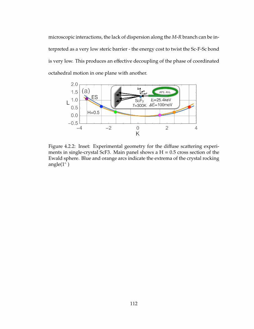
microscopic interactions, the lack of dispersion along the M-R branch can be in-
terpreted as a very low steric barrier - the energy cost to twist the Sc-F-Sc bond
is very low. This produces an effective decoupling of the phase of coordinated
octahedral motion in one plane with another.
Figure 4.2.2: Inset: Experimental geometry for the diffuse scattering experi-ments in single-crystal ScF3. Main panel shows a H = 0.5 cross section of theEwald sphere. Blue and orange arcs indicate the extrema of the crystal rockingangle(1 )
112

Figure 4.2.3: (a) Diffuse scattering intensity collected using the experimentalgeometry in Figure 4.2.2. Mid-zone intensity at M points are indicated bydashed circles and are found in almost every BZ. Dashed lines indicate cutsthrough the intensity patterns shown in (b). Each cut in (a) is taken an anequivalent K value but corresponds to a different L value. The negligiblechange in widths is strong evidence of 2D spatial correlations.
113

Chapter 5
Two dimensional constrained lattice model to studyScF3 lattice
5.1 Introduction
In this chapter we address the extent to which rigid octahedral motion de-
scribes the dynamical fluctuations behind NTE by generalizing a simple model
supporting a single floppy mode that is often used to heuristically describe
instances of NTE. We also discuss the tendencies of this model toward dy-
namic inhomogeneities and its application to thermal diffuce scattering data
presented in Chapter 4.
Figure 5.1.1b shows the simple cubic BZ of ScF3 with break outs indicating
the nature of the correlated motion comprising M-R zone boundary modes.
The experimentally-observed (Chapter 4) decoupling of coordinated rotations
within planar manifolds suggests there is prominent importance of the lattice
dynamics of a 2D section, shown in Figure 5.1.2a,b. A model consisting of
stiff diamonds connected by hinged joints shown in Figure 5.1.2a,b appears
in numerous contexts in the literature describing the NTE phenomenon as a
physical model wherein one may understand that collective motion of a rigid
114

network can generically provide a NTE influence[80, 79, 81]. The diamonds
could represent metal-anion octahedra in the structural NTE perovskites ScF3
or ReO3, but the idea has been used to describe more complex structures[79, 170,
171, 80, 81]. Here, we momentarily enforce the rigidity of the molecular units
in an analysis of this two-dimensional constrained lattice model (2D CLM) to
study the rigid limit expectations before comparing to experiment in order to
provide insights into the limitations and strengths of rigid models in the NTE
problem
Figure 5.1.1: (a) A 5 × 5 × 5 crystallite of ScF3 in the average structure (125octahedra). (b) The hollow cube shows the simple cubic BZ with shadedregions indicating the positions of observed scattering rods from the data inFigure 4.2.3. Breakouts show possible real-space staggered rotation patternswhich preserve internal octahedral dimensions at the indicated high-symmetrymomentum-space points. Red and blue shading in the diamonds indicate equalbut opposite magnitudes of rotation.
5.2 Two-dimensional constrained lattice model
The 2D CLM consists of corner-linked diamonds with coordinate origin at its
115

Figure 5.1.2: A model consisting of stiff diamonds connected by hinged jointsshown. As a result of the constraints, a staggered rotation by an angle θ in (b)causes a shortening of the vector locating each diamond by a factor cos θ
center of mass (COM). The N = NxNy diamonds are attached by hinged joints,
so that their motional degrees of freedom are constrained. The CLM is isostatic,
or marginally constrained, in the sense that even in the thermodynamic limit,
there is exactly one internal degree of freedom: a staggered rotation of each dia-
mond by an angle . Increasing θ from zero contracts the lattice from initial area
A0 to an area A0 cos2 θ, and thermal activation of this collective mode is often
attributed as the origin of NTE [80, 172, 170, 171]. Efforts to expand this model
to field theories which respect the high-energy constraints of bond-stretch and
bond-bend degrees of freedom include mimicking polyhedral pliancy through
a split-atom approach [164], by lowering the degree of constraint [51, 165],
or permitting some diamonds to be replaced by springs [166], and unusual
properties such as NTE are found in each case. When there is no staggered
116

rotation, θ = 0, and a diamond center can be located at position r(θ = 0) =
(nx,ny)a0. When θ , 0, the distance between neighboring diamond centers is
reduced by a multiplicative factor cosθ and each position vector is scaled simi-
larly −→r (θ)=(nx,ny)a0 cosθ with velocity −→r (θ) = −(nx,ny)a0θ sinθ. The velocity
vectors of each diamond always point directly toward or away from the COM.
The total translational kinetic energy summed over all diamonds in the crystal
is:
Ktrans
=12
Icθ2 sin2 θ (5.2.1)
where Ic =∑
nxnym((nxa0)2 + (nya0)2) is the moment of inertia of a similar crystal
where diamonds are replaced by points, each of mass m.
Including the rotational kinetic energy of each diamond and summing, the
total kinetic energy of the 2D CLM is
K =12
NIθ2 +12
Icθ2 sin2 θ =
12
NIθ2(1 + k2 sin2 θ) (5.2.2)
where k=√
IcNI
=√γN and γ depends on the aspect ratio of the crystal
and mass distribution for the diamonds (' 1.79 for a square crystallite of
ScF3). Finally, we introduce the lowest Fourier component of an intermolecular
bond-bending potential at the hinges κ(1 − cosθ) to stiffen the structure from
collapse. Microscopically, this influence arises from a competition between
mutual repulsion of like charges including dipolar contributions and anion
117

polarizability and is considered low for trifluorides with a large B-site atomic
radius such as Sc [106]. The total energy, expanded for a small angle to the
harmonic case, is then
E=12
NI(1 + k2 sin2 θ)θ2 +12
Nbκθ2 (5.2.3)
where Nb ' 2N is the total number of intermolecular linkages. One may view
Equation 5.2.3 as a generalization of a harmonic oscillator (k→ 0) describing
a residual degree of freedom resultant from integrating out high-energy bond-
stretch and bond-bend degrees of freedom.
Significantly, the total effective inertia of the FM has a rotational part (the
first term) which scales with system size in an intensive way (∝ N), while the
translational kinetic energy scales extensively (Ic ∝ N2). As the thermodynamic
limit is approached, molecular units at the boundary of a free crystallite must
traverse macroscopic distances within a single FM cycle while experiencing
enormous force gradients, pointing to a necessary breakdown of rigidity and
falsifies the rigid approach on physical grounds. A homogeneous FM in an
infinite system therefore has an infinite kinetic energy density, and the effect
favors inhomogeneous spatial textures through intramolecular deformations
at a penalty of elastic potential energy. In what follows we entertain the
possibility that the nanoscale correlations we observe are a signature of such a
breakdown, as an alternative approach to a conventional phonon population
118

of optical modes.
In the limit of small-angle and large system size (k), one can integrate Equation
5.2.3 to find
(t − t0)2
(kθ0/ωp)2 +θ2
θ20
=1. (5.2.4)
where θ0 is the amplitude and ωp=√
Nbκ/NI=√
g/R is the angular frequency
of small oscillations in the limit k=0. Several aspects of the thermodynamic FM
are distinct from the harmonic case: (i) The period τ = 4kθ0ωp
= 4θ0
√Ic
Nbκdiverges
and is proportional to the amplitude of oscillation, (ii) the time-averaged clas-
sical probability distribution P(θ) dwells much longer near the extrema than
the harmonic case, and (iii) the system spends a vanishingly small time in the
average structure θ = 0 (Figure 5.2.1b). The latter two points are apparent in
recent molecular dynamics simulations of ScF3 that reach similar surprising
conclusions of nearly vanishing probability for straight Sc-F-Sc bonds at ele-
vated temperatures [173]. A physical expression of this peculiar distribution
in the present model can be seen in the time-averaged area, related to the
moments of this distribution, 〈A〉t = A0〈cos2 θ(t)〉t = A0(1 − ηθ20), where η=1/2
for the sinusoidal k = 0 case and η=2/3 for the thermodynamic limit k → ∞
4, showing that the strain dynamics of the 2D CLM enhances NTE over its
harmonic counterparts. The lessons from these results on the CLM is that the
The area of the 2D lattice at time t is given by A(t) = NxNy cos2 θ(t) ∼ NxNy
(1 − θ(t)2
). Time
119

collective motion of the dilating FM is slow and anharmonic, dwelling near
extrema as a feature of its dynamics.
Figure 5.2.1: (a)(d) show classical solutions for θ(t) which follow from Equation5.2.3. These are plotted for different values of k0, which uniquely quantifiesthe anharmonic behavior. The time axes in (a) and (c) are scaled by the FMperiod
We note that the dispersion away from the zone boundaries is very steep,
approaching the longitudinal acoustic velocity, suggesting the dominant im-
portance of the BZ edge modes to NTE. We are therefore positioned to compare
the experimental a(T) for ScF3 with that of an uncorrelated stack of N = N2x
averaging θ(t)2 over a period τ for both the harmonic and circle wave limits:
〈θ2〉t,harm =
1τ
∫ τ
0
(θ0 cos
(2πtτ
))2
dt =12θ2
0
〈θ2〉t,circ =
1τ
∫ τ
0
θ0
√1 −
( tτ
)2
2
dt =23θ2
0
The circle wave limit spends significantly more time near the extrema than the harmonic case,resulting in a larger time averaged value for 〈θ2
〉t. Hence, the NTE effect due to FM oscillationsis amplified for larger systems exhibiting stronger anharmonicity.
120

thermally averaged 2D CLMs of area A(T) = A0〈cos2 θ〉T ' A0(1 − 〈θ2〉T). The
lattice parameter of the stack is then a(T) = a0〈cos2 θ〉1/3T ' a0(1−〈θ2〉T/3), where
we sum over the BZ edges to obtain
〈θ2〉T =
1Z
∫∞
−∞
dθdLθθ2e−βH =2kBTNbκ
1
1 + K0(δ)K1(δ)
, (5.2.5)
β=1/kBT, Z is the classical partition function, δ = Nbκ4k2kBT =
Iω2p
4kBTγ , and Kn(δ) is the
order n modified Bessel function of the second kind.
5.3 Application of model to experimental results
We determined a(T) and the transverse anion thermal parameter U33(T) =
(a0/2)2〈θ2〉T using model and the plots (Figures 5.3.1a and 5.3.1b) are shown
along with existing experimental data [23, 160] using the observed Nx = 5.5 for
different values ofωp. The inertial parameters for ScF3 and a0 = 4.0285 Å is used
Best agreement is met when ~ωp ' 1.6 meV, which is similar in magnitude to the
observed branch energy at low temperature (1.2-1.4 meV) and somewhat lower
than the observed values at ambient temperature (3.43.6 meV). We remark that
existing computational work gives mode energies ranging from 3 to 6.5 meV
[161, 68, 160], and that inclusion of other low-energy modes off of the high-
symmetry cut is expected to raise this effective energy scale somewhat.
Remarkably, this analysis has the implication of an intricate link between the
following experimental quantities: (i) the length scale ' 6 unit cells we observe
121

in diffuse x-ray scattering, (ii) the energy scale ' 1 meV for the M − R branch
reported using IXS, and (iii) the degree of dimensional fluctuation measured
through the coefficient of thermal expansion measured using x-ray diffrac-
tion. Recent purely theoretical analyses of square and kagome lattices crossing
the isostatic limit using different approaches have also pointed to emergent
nanometer length scales [174, 175, 117]. In contrast, the present results use a
simple approach motivated by experimental observations to relate disparate
experimental observables in a real material system.
Recent classical molecular dynamics simulations and general arguments have
suggested the strict rigidity of molecular units is not possible or necessary
for NTE [167, 135, 160, 168], fully consistent with the finite correlation length
implied by our experiments and divergent kinetic energy density in the ther-
modynamic limit of the CLM. Here we propose a mechanism of strain relief
and kinetic energy lowering consistent with experiments, the quantized nature
of the vibrational spectrum, and the hierarchy of stiffness present in the bond
patterns. The pileup of translational kinetic energy at the boundary of a di-
lating region implied by molecular rigidity could be alleviated by introducing
bond-bend intramolecular polyhedral deformations. Within a FM cycle, the
separation between the edges of two adjacent, dilating nanoregions is mini-
mized if the phases of oscillation ϕ1 and ϕ2 differ by ϕ1 − ϕ2 = ±π/2. These
two choices keep the edges in contact without parting the junction and lower
the translational kinetic energy significantly. We can demonstrate this savings
122

Figure 5.3.1: (a) Lattice parameter of ScF3 below T = 300 K from Ref. [23](b) Transverse fluorine thermal parameter determined from x-ray pair densityfunction analysis [18]. Superimposed on (a) and (b) are the correspondingquantities from (2) using Nx = 5.5 for varying values of ~ωp (c) Velocity fieldsuperimposed on a homogeneously excited FM, with phase and kinetic energybelow. (d) shows the significant kinetic energy lowering when a π/2 defect isintroduced.
by considering the kinetic energy of a homogeneous excitation of a 2D CLM in
a long, narrow solid shown in Figure 5.3.1, Nx × Ny, with Nx >> Ny is given
in Equation 5.2.2 with moment of inertia I(1)c = 2ma2N3
xNy/3.An inhomoge-
neous excitation with a domain wall at the origin separating a region of FM
phase 0 (maximum volume) for x > 0 and FM phase π/2 (minimum volume)
123

for x < 0 has an effective crystal moment of inertia which is 4 times lower
I(2)c = ma2N3
xNy/6 = 14 I(1)
c . A similar calculation for two semiplanes in contact
gives I(2)c = 1
2 I(1)c , in any case lowering the energy. The interface between these
regions must feature excited optical modes with an elastic energy penalty made
possible by the enormous lowering of translational kinetic energy.
The molecular velocity field in this scenario may be described as monopole-
antimonopole pairs. The topological defects proposed here are resultant from
the alleviation of strain at the interface and are protected at a ' 20 meV scale.
While details of a possible superstructure await further experiments and mod-
eling, we identify a large kinetic energy lowering occurs through the formation
of aπ/2 phase slip defect, which may pose intrinsic challenges to theories which
embark with a classical approach. For a large single 2D planar section, the±π/2
phase slip could occur in multiple ways, potentially benefitting the stability of
the proposed excitations. A three-dimensional extension of such defect field is
beyond the scope of the present work, but may give rise to nontrivial topolog-
ical textures in the phase field of the FM, raising the interest in lattice systems
with unconventional dynamics. Future time-resolved and coherent x-ray scat-
tering experiments are likely to address the phase relationship intrinsic to the
nanoscale correlations in NTE materials.
124

Chapter 6
Infrared study of ScF3
6.1 Introduction
Even though it is arguable that the molecular rigidity decides the NTE on frame-
work structures [68, 160, 168, 167], studies have shown that coordinated tilt pat-
tern of octahedra [169] is common among ReO3 type structures of space group
Pm3m. These coordinated motions are identified as low energy modes hence
known as soft modes and correspond to Brillouin zone(BZ) edge of simple cu-
bic BZ. Further experimental evidences supported by theoretical modeling [48]
has proposed that these soft modes can possibly relate with two-dimensional
nanoscale correlations exist at momentum-space region.
It is clear that the dynamics of the ScF3 structure and it’s properties are mostly
discussed in connection with the degrees of freedom associated with off center
of the BZ. Here we make an attempt to investigate zone center optical phonons
in order to find if any correlation exists between zone center and off-zone
center phonon modes and to study the temperature dependence optical prop-
erties by using infrared (IR) reflectance and time domain terahertz(TD-THz)
transmission spectroscopy.
125
6.2 Measurements
IR measurements were carried out using single crystal ScF3. Sample was
polished and half of the polished surface was coated with gold using standard
metal evaporator in the laboratory at the Department of Physics at University
of Connecticut. The amount of gold was chosen such that the thickness of gold
layer was higher than that of the skin depth for far-IR radiation which is about
50 nm .
Far-IR reflections were measured using Bruker 66v Fourier Transform Infrared
Spectrometer(FTIR) in the laboratory. Sample was kept under vacuum in an op-
tical continuous flow cryostat runs with liquid helium and sample temperature
was measured using Cernox sensor mounted near the sample. Temperature
was recorded in the range of 30 - 300 K. The spectra was collected with a
bolometeric detection covering the range of frequencies 100 - 1000 cm−1 using
a multilayer beam splitter(T222) and a glow-bar as the source of radiation.
To investigate optical properties at further low frequencies, we performed TD-
THz spectroscopy. Laser pulses (Pulse width = 70 fs) produced by KMLabs
Griffin -10 Ti:Sapphire pulsed laser system were directed to broad area inter-
digital photoconductive THz antenna from BATOP optoelectronics in order
to generate THz radiation in the range of 10 - 80 cm−1. THz detection was
achieved with electro-optic sampling method by using 〈100〉- oriented ZnTe
crystal. The spectrometer was purged with dry nitrogen air. Single crystal ScF3
126

sample with dimensions of 4.7 mm×4.24 mm×3.59 mm was taped onto the
sample holder at the edges. The sample chamber which consits of two kapton
windows was kept under high vacuum and was attached to vibration-free,
cryogen-free optical cryocooler. Measurements were taken down to 30 K.
6.3 Lorentzian model fitting
The most common way to fit dielectric dispersion in ordinary crystals is the
three-parameter model, where the dielectric function is modeled by the sum of
independent damped harmonic oscillators(Lorentzians),
εr(ω) = ε∞ +∑
n
ω2pn
ω2TOn − ω
2 + iωγTOn(6.3.1)
where ε∞ is the high-frequency (electronic) dielectric constant,ωpn is the plasma
frequancy of the n-th transverse vibrational mode of frequancy ωT0n and γn is
its damping constant or line width.
Consider an atom and assume that the nucleus mass is massive compared with
electrons. We can treat the electrons in the atom are connected with springs to
the nucleus. So the motion of an electron is described by a damped harmonic
oscillator and we can write
md2r(t)
dt2 + mγdr(t)
dt+ mω2
0r(t) = −eE(t) (6.3.2)
where the second term represents the damping with damping constant γ and
127

the third term represents the Hooke’s law restoring force with characteristics
frequency ω0. Last term is the force on the electron due to local electric field
E. The interaction of the electron with magnetic field has been neglected here.
Assuming the solution r(t) = r0eiωt the local electric field varies as E(t) = E0eiωt.
By applying this to the above equation we could obtain the local polarization
or induced dipole moment
p = er0 =e2E0
m1
ω20 − ω
2 − iωγ(6.3.3)
The total polarization, P = 〈N〉p, where N is number of atoms per unit volume.
Further P = ε0χE, where electric susceptibility χ = εr − 1. Here εr is relative
dielectric permitivity which is in general a complex number and frequency
dependent. By taking all this in to account we can write down
εr(ω) = 1 +Ne2
mε0
1ω2
0 − ω2 − iωγ
. (6.3.4)
By introducing oscillator strength ωp = (Ne2/mε0)1/2 and considering total of n
electrons per atom
εr(ω) = ε∞ +
n∑i=1
ω2pi
ω20i − ω
2 − iωγi. (6.3.5)
6.4 Factorized model fitting
128

However four parameter factorized form of dielectric function has long been
discussed[176, 177, 178], especially to model ionic crystals[179, 176, 180] with
large LO-TO splitting. It is advantageous to use the model since it allows
different damping constants hence different relaxation time for the LO and TO
phonon modes as stated below.
εr(ω) = ε∞∏
n
ω2LOn − ω
2 + iωγLOn
ω2TOn − ω
2 + iωγTOn(6.4.1)
where ωTOn is n-th transverse vibrational mode and ωLOn is n-th longitudinal
vibrational mode. γLOn and γTOn are corresponding damping coefficients.
The complex permitivity in a material is directly proportional to the suscepti-
bility which is a measure of the polarizability of the materials for an external
electric field. In general permitivity depends on frequency of applied electric
field(Equation 6.3.5) and the atomic structure or in other words how strongly
the electrons bound into the atom. Therefore optical properties such as optical
conductivity, refractive index, absorption coefficient are directly related to ma-
terials complex permitivity. When electromagnetic waves interact with matter
they undergo various phenomena such as transmittance, absorption, reflec-
tions etc. and such phenomena are governed by so called optical properties
of materials. Therefore experimentalists use different experimental techniques
to measure the above mentioned phenomena and are successfully able to un-
derstand the fundamentals of material behaviors by studying their optical
129
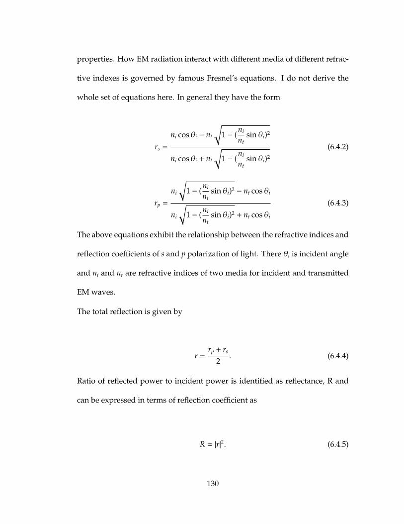
properties. How EM radiation interact with different media of different refrac-
tive indexes is governed by famous Fresnel’s equations. I do not derive the
whole set of equations here. In general they have the form
rs =
ni cosθi − nt
√1 − (
ni
ntsinθi)2
ni cosθi + nt
√1 − (
ni
ntsinθi)2
(6.4.2)
rp =
ni
√1 − (
ni
ntsinθi)2 − nt cosθi
ni
√1 − (
ni
ntsinθi)2 + nt cosθi
(6.4.3)
The above equations exhibit the relationship between the refractive indices and
reflection coefficients of s and p polarization of light. There θi is incident angle
and ni and nt are refractive indices of two media for incident and transmitted
EM waves.
The total reflection is given by
r =rp + rs
2. (6.4.4)
Ratio of reflected power to incident power is identified as reflectance, R and
can be expressed in terms of reflection coefficient as
R = |r|2. (6.4.5)
130

For almost normal incidence of light θi = 0 and both polarizations have the
same contributions to the reflectance. I should also emphasize that in general
refractive index of a material is complex and frequency dependent hence it is
more accurate to denote it as n(ω). When an EM wave incident normal to the
interface between air and a medium of refractive index n(ω)) the reflectance
can further be simplified to
R =
∣∣∣∣∣ n(ω) − 1n(ω) + 1
∣∣∣∣∣2 . (6.4.6)
Materials refractive index n(ω) =√εr(ω).µr(ω). For non magnetic material
µr(ω)=0. Therefore the reflectance can be represented in terms of frequency
dependent permitivity, εr(ω) such that
R =
∣∣∣∣∣∣∣√εr(ω) − 1√εr(ω) + 1
∣∣∣∣∣∣∣2
(6.4.7)
The relationship between the measured reflectance,R and the models discussed
earlier infers from equations 6.3.5, 6.4.1 and 6.4.7.
We analyzed our data shown in Figure 6.6.1 using both Lorentzian oscillator
model and factorized form model mentioned earlier. The Chi squared valued
from best fit was obtained and factorized formula better fits with data with
lower Chi squared. The best fit parameters obtained at 300 K are tabulated in
Table 6.6.3 for comparison. Figure 6.4.2 compares the TO frequencies obtained
131

Figure 6.4.1: A sample spectra taken for ScF3. The frequency-dependent opticalbehavior of ScF3 is divided in regions: T for transmission (or ”transparency”),A for absorption and R for reflection.
from both models. We see a strong absorption feature in the broad reststrahlen
band in our data. Therefore we added one additional oscillator(total of three
oscillators in both models) in the fitting process. The implication of this is
discussed later in this chapter. Fit to 300 K data estimated the ε∞ to be 1.92 and
it was used for low temperature fittings as a fixed parameter.
6.5 Zone center modes
The cubic structure of perovskite ScF3 belongs to Pm3m space group .The
Sc atoms and F atoms occupy the Wyckoff positions 1a(0,0,0) and 3d(1/2,0,0)
corresponding with the point group Oh. Four atoms per unit cell suggests
12 branches in which 3 of them are acoustics. The irreducible representation
of normal mode vibrations at the BZ center of the point group has the form
132

Figure 6.4.2: Compare the parameters obtained from factorized form modeland Lorentzian model. Black markers are obtained from lorentzian model andcolored plots are from factorized form model.
Γ0 = T2u + 3T1u [95]. Out of them T2u + 2T1u are optical modes and 2T1u are
identified as IR active modes. None of the modes are Raman active while T2u
mode is neither Raman nor IR active and is known as “silent mode”. None
of the mode is Raman active while T2u mode is neither Raman nor IR active
which is known as silent mode. For non polar crystals the IR active modes are
triply degenerate with two transverse optical(TO) modes and one longitudinal
optical(LO) mode in each branch. But in case of polar crystals like ScF3 the TO
and LO modes are split at ZC due to the well-known phenomenon which the
displacement of charges in long wave length LO modes create dipole moments.
The electric field induced by dipole moment has additional contribution to the
restoring force hence the LO mode has higher energy than TO mode. This is
known as LO-TO splitting.
133

Figure 6.5.1: Gray sphere represents Sc atom while Blue spheres represent Fatoms. Black arrows show the direction of displacement. (a) Acoustic mode.(b) The lowest energy optical mode. This is also known as silent mode (c) Thehighest energy mode (TO2 in our case) (d) The low energy mode which is alsoknown as breathing mode.(TO1 in our case)
ScF3 has no Raman-active modes under ambient pressures owing to its cubic
symmetry. However at 0.6 GPa, the staggered octahedra tilt around 〈111〉 and
the structure corresponds to rhombohedral phase which results in Raman ac-
tive modes. More interestingly the rhombohedral structure undergoes second
structural transition at about 3 GPa.
6.6 Infrared measurement results
Reflectivity data along with the best fits of equation 6.4.1 are plotted in Figure
6.6.1 in the temperature range 30-300 K for ScF3. Reflectivity clearly indicates
134

two restsrahlen bands as predicted by group theory of the crystal symmetry.
Increase in reflectivity on cooling due to reduced scattering (reduced damping
constant) at low temperatures are clearly visible.
Previous [161] IR absorption spectra on ScF3 powder sample has shown two ab-
sorption bands at 220 cm−1 and 520 cm−1 which correspond to Sc-F-Sc bending
and Sc-F stretching respectively. Simulations performed beyond quasi har-
monic approximation has successfully reproduced experimental values such
as lattice parameter, energy gap and lattice dynamics in ScF3. Bond stretching
modes get softer as the temperature is increased and bond bending modes get
stiffer as temperature goes up but both modes are shifted about 6 cm−1 within
300 K temperature window.
Figure 6.6.1: Measured reflectance of ScF3 sample at different temperatures
135

Model ωTO1 ωLO1 γTO2 γLO2
———————— —————–——————–—————-————–Factorized formula 214 277 9.05 8.61
493 675 16.07 19.95592 587 47.64 45.31
Lorentzian 214 8.57493 - 16.6 -590 - 49.8 -
Table 6.6.3: Compare the fit models at 300 K. Unites are given in cm−1
Our results are agreed well with most of the calculations and comparison is
tabulated in Table 6.6.4. As seen in Figure 6.6.2(c) the low energy TO mode
of Sc-F-Sc bond bending mode stiffen about 3 cm−1 as the temperature in-
creases within 270 K temperature window. From here onwards, this mode is
called as TO1. The highest energy TO mode(TO2) or stretching mode soften
by 5 cm−1(Figure 6.6.2(a)). The values obtained from Kramers-Kronig consis-
tent analysis are somewhat difference than the values published from powder
transmission measurements [161] which may result from the single crystalline
nature. The low and high energy LO phonons (LO1 and LO2) exhibit similar
behavior as the TO phonons. Figure 6.6.2(b) and Figure 6.6.2(d) plots temper-
ature dependence of LO mode frequencies.
Further, temperature dependence ε(ω) was obtained and the infrared absorp-
tion, Im(ε(ω)) and infrared loss function, Im(-1/ε(ω)) are plotted in Fig. 3. The
peak values corresponds to TO and LO phonons respectively
Around 600 cm−1, a dip can be seen in the reststrahlen band, indicating addi-
tional absorption in ScF3. This has been previously observed in many fluoride
136

Source ωTO1 ωLO1 ωTO2 ωLO2
—————————————–——————–—————-————–Ours ∼ 214 ∼ 277 ∼ 493 ∼ 675
Calculations[161] ∼ 215 ∼ 275 ∼ 485 ∼ 695Calculations[68] ∼ 190 ∼ 359 ∼ 496 ∼ 665Calculations[99] ∼ 200 - ∼ 450 -
Calculations[181] ∼ 211 ∼ 154 ∼ 477 ∼ 590
Table 6.6.4: Comparison of our experimental results with previous calculationsat 300 K. Units of energies are cm−1.
systems such as RbCaF3, CsCaF3, KZnF3 [182], CaF2, SrF2, BaF2 [?], LiF [183, ?]
and NaF [?]. In case of LiF Willett-Gies and co authors have assigned the
feature to two phonon absorption process following Eldridge [?] and in other
cases it was assigned to multiphonon absorption. Best fits in most cases were
obtained by fitting data with factorized formula. The temperature dependence
of ScF3 multiphonon absorption is larger than the single phonon absorption
and softens about 11 cm−1 within 270 K temperature interval. .
In general the poles of ε(ω) in Eqn. 2 are identified as TO phonon energies
and zeros of ε(ω) represent energies of LO phonons. But according to Berre-
man and Unterwald [176] if they are much closer to one another they only
produce weak absorption in dispersion curve and can be depicted to two or
more phonons. Therefore the weak absorption feature appeared around 600
cm−1(Figure 6.6.3(b)) which corresponds to the third pole of ε(ω) in Equation
6.4.1 is assigned to a multiphonon process. The zero counterpart is found in
loss function as shown in Figure 6.6.3(a).
6.6.1 Discussion
137

Figure 6.6.2: (a),(c) TO phonon energies & (b),(d) LO phonon energies obtainedfor ScF3 by fitting the reflection with factorized formula at different tempera-tures. Corresponding linewidths obtained are shown in insets
The large ionicity in ScF3 could be the reason for broad bands of LO-TO split-
ting. Highest LO mode energy for ScF3 is 675 cm−1 and for LiF, LO energy was
found to be 669 cm−1[183]. Since ScF3 ionicity is comparable to that of LiF one
could expect this.
Highest TO and LO modes are associated with bond stretching modes. Soft-
ening of the modes as temperature in increased can be attributed to weaken
138
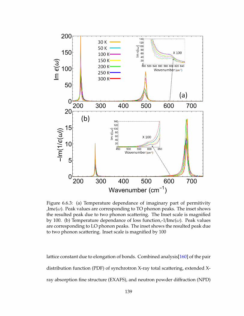
Figure 6.6.3: (a) Temperature dependance of imaginary part of permitivity,Imε(ω). Peak values are corresponding to TO phonon peaks. The inset showsthe resulted peak due to two phonon scattering. The Inset scale is magnifiedby 100. (b) Temperature dependance of loss function,-1/Imε(ω). Peak valuesare corresponding to LO phonon peaks. The inset shows the resulted peak dueto two phonon scattering. Inset scale is magnified by 100
lattice constant due to elongation of bonds. Combined analysis[160] of the pair
distribution function (PDF) of synchrotron X-ray total scattering, extended X-
ray absorption fine structure (EXAFS), and neutron powder diffraction (NPD)
139
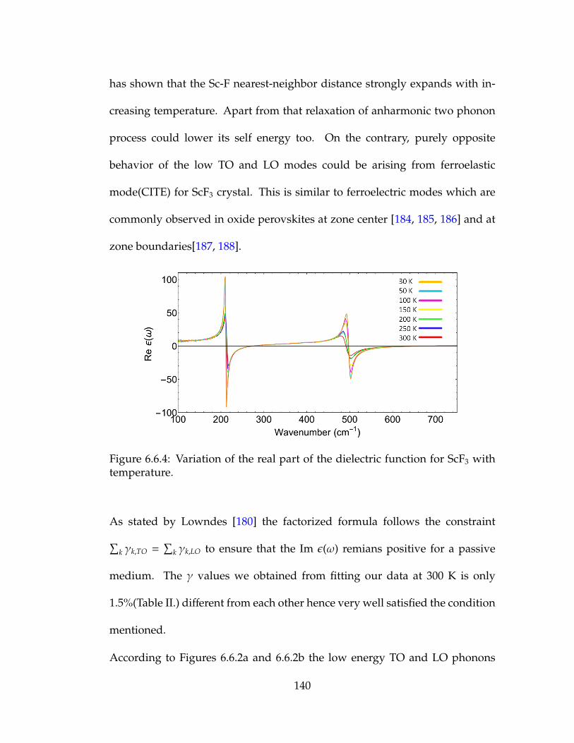
has shown that the Sc-F nearest-neighbor distance strongly expands with in-
creasing temperature. Apart from that relaxation of anharmonic two phonon
process could lower its self energy too. On the contrary, purely opposite
behavior of the low TO and LO modes could be arising from ferroelastic
mode(CITE) for ScF3 crystal. This is similar to ferroelectric modes which are
commonly observed in oxide perovskites at zone center [184, 185, 186] and at
zone boundaries[187, 188].
Figure 6.6.4: Variation of the real part of the dielectric function for ScF3 withtemperature.
As stated by Lowndes [180] the factorized formula follows the constraint∑k γk,TO =
∑k γk,LO to ensure that the Im ε(ω) remians positive for a passive
medium. The γ values we obtained from fitting our data at 300 K is only
1.5%(Table II.) different from each other hence very well satisfied the condition
mentioned.
According to Figures 6.6.2a and 6.6.2b the low energy TO and LO phonons
140
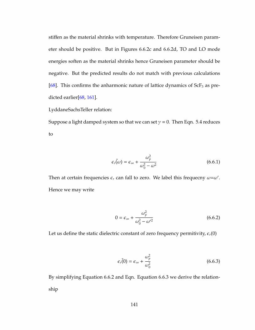
stiffen as the material shrinks with temperature. Therefore Gruneisen param-
eter should be positive. But in Figures 6.6.2c and 6.6.2d, TO and LO mode
energies soften as the material shrinks hence Gruneisen parameter should be
negative. But the predicted results do not match with previous calculations
[68]. This confirms the anharmonic nature of lattice dynamics of ScF3 as pre-
dicted earlier[68, 161].
LyddaneSachsTeller relation:
Suppose a light damped system so that we can set γ = 0. Then Eqn. 5.4 reduces
to
˜εr(ω) = ε∞ +ω2
p
ω20 − ω
2(6.6.1)
Then at certain frequencies εr can fall to zero. We label this frequecny ω=ω′.
Hence we may write
0 = ε∞ +ω2
p
ω20 − ω
′2(6.6.2)
Let us define the static dielectric constant of zero frequency permitivity, εr(0)
˜εr(0) = ε∞ +ω2
p
ω20
(6.6.3)
By simplifying Equation 6.6.2 and Eqn. Equation 6.6.3 we derive the relation-
ship
141

ω′2 = ω2TOεr(0)ε∞
(6.6.4)
To understand the physical meaning of the frequency ω2 at εr(ω)=0 consider
the guess law. In a medium with no free charges the guess law reads
∇.D = ∇.(εrε0E) (6.6.5)
Generalized form of electric field propagates through a medium is given by
E(r, t) = E0ei(k.r−ωt) (6.6.6)
When we apply the EM wave form into Equation 6.6.5 we assume that εr , 0.
Therefore we conclude that k.E = 0 and hence determine that the wave vector
is perpendicular to that of electric field. But if εr=0, we can conclude that k.E ,
0. These types of waves are known as longitudinal waves. So we can write
down Equation 6.6.4 as
ω2LO = ω2
TOεr(0)ε∞
(6.6.7)
This relation is known as Lyddane-Sachs-Teller(LST) relation, which is com-
monly presented in the form
142

εr(0)ε∞
=ω2
LO
ω2TO
(6.6.8)
It is also known [177, 189] for high symmetric crystals and for N number of
optical modes the LST relation becomes
εr(0)ε∞
=
N∏i=1
ω2LOi
ω2TOi
(6.6.9)
Obtaining εr(0) for ScF3:
The simple relation given in Equation 6.6.9 is used to derive εr(0) for ScF3. It
is also important to realize that the terms zero frequency relative permitivity,
static relative permitivity or static dielectric constant are used to identify the
same quantity, εr(0). The capacitance of a capacitor is directly proportional to
the static dielectric constant of the dielectric. The static dielectric constants for
ScF3 is almost temperature independent and are tabulated in Table 6.6.5. We
use ε∞ =1.92 which is obtained from fitting the data to factorized form model.
Temp(K) εr(0) Temp(K) εr(0)—————————-—————————– ————————— ——-30 6.04 200 6.0350 6.04 250 6.0270 6.05 300 6.01100 6.03
Table 6.6.5: Static dielectric constant for ScF3 obtained from LST relation
One of the main objective of our measurement is to figure out if any correlation
exists between the lowest energy mode in zone boundary M − R branch and
143

zone center optical phonons. At 300 K the two phonon absorption is observed
at 592 cm−1 and within 270 K temperature window the corresponding energy
decreases about 11 cm−1 as the temperature increases.
Assigned Combined energy Our expt. resultsphonon pair from calc.—————————-————————— ————————-TO(X) + TA(X) ∼ 547.4 [161] ∼ 592TO(M) + TA(M) ∼ 597.5 [161] ∼ 592TO(X) + LA(X) ∼ 639.8 [161] ∼ 592TO(X)bend + LA(X) ∼ 632.6 [161] ∼ 592
Table 6.6.6: Two phonon absorption possibilities, if only high symmetric pointsare considered
Szigeti[190] and Lax and Burstein [191] have shown that the sum and difference
processes of lattice vibrations could arise from the second order dipole moment
and third order anharmonic interactions by studying the effect of these interac-
tions on IR and Raman spectra. If that is the case the multiphonon absorption
feature can be assigned into two-phonon absorption which then can be view in
two different ways. It could be either a summation process such as two phonon
creation or difference process such as creation and annihilation of an existing
phonon.
The phonon creation and annihilation is possible but it would require a com-
bination of LO2 mode with other lower mode. The possibility of LO2 mode
involvement in the two phonon absorption is omitted since it is not possible to
create longitudinal modes with almost normal incident reflection. Apart from
that the fact that the two-phonon absorption feature in IR data doesn’t smear
144

out as the temperature is lowered suggests that it only involves two-phonon
emission(sum) mode, rather than emission and absorption(difference) mode.
Figure 6.6.5: Most probable combination of two phonons are shown. Theycould be arising from sharp DOS which is shown in extended blue area incombined plots of phonon dispersion and corresponding DOS. Directions alongΓ - M - R and along Γ - X - M are considered. A mode lies at momentumpoint -q with in red( at momentum point q in green) areas of dispersion plotcorresponding to higher energy DOS peak and a mode lies at momentum pointq with in red( at momentum point -q in green) areas in the lower energy DOSpeak excite and correspond to two phonon absorption. Dispersion plots aretaken from [24]
.
One set of possibility of two phonon creation is a combination of TO1 mode
at momentum q with different low energy mode at momentum -q. From
the measurement we found that the TO1 mode stiffen with temperature by 3
cm−1. In order to satisfy energy conservation the second phonon involve in the
process should soften by about 14 cm−1( -11(two phonon) = + 3 (TO1 mode) -
14 ). According to the literature [24, 68] none of the branches soften this much
145

within 300 K range as temperature is increased. Therefore we could omit the
possibility of TO1 mode involvement in two phonon absorption.
The other possibility of two phonon feature is TO2 phonon is excited at mo-
mentum q while another low energy phonon is excited at momentum -q. The
DOS around TO2 mode(hardest TO mode) is very narrow and hence almost
dispersionless through out the first BZ. Therefore the second phonon can arise
from any where in the BZ such that the momentum is conserved. In order to
satisfy the energy conservation the other phonon mode should have energy
around 100 cm−1. Calculation and experimentation results[68, 161, 24] show
five noticeable peaks in ScF3 phonon density of state(DOS). They are related
to five optical phonon branches(degenerated TO, splitted TO - LO pair). The
lowest peak of density of states obtained by Li et al.[68] centers at 13 meV(104
cm−1) which very much satisfy the energy requirement of the second phonon.
Therefore we conclude that TO2 mode and any mode corresponds to reciprocal
space points in the whole X - M, Γ - M and Γ - R branches can combine in order
to give two phonon absorption in ScF3. If we only consider the high symmetry
points then the possibilities gets narrow down to a few as shown in Table 6.6.6.
146

Chapter 7
Resonant Ultrasound Spectroscopy
7.1 Introduction
Resonant Ultrasound Spectroscopy(RUS) is an ultrasonic used measurement
technique which was fully developed in late 80s. Ultrasonic measurements
provide valuable information on elasticity related properties of solids such as
elastic constants, shear modulus, young’s modulus,bulk modulus and poisson
ratio etc. RUS has distinctive advantages over all the other methods which
could be used to carry out these types of measurements. More importantly RUS
requires very less amount of materials in order to achieve accurate results and
one good spectrum may be more than enough to fully characterize the elastic
properties of a given sample. Another great aspect is RUS measurements
are fast, nondestructive and result in very less time consuming experiment.
The most challenging part of RUS experiment is data interpretation, which
usually involves solving few algorithms to back calculate elastic properties
using measured normal mode frequencies and material geometry. Advances
of computer programming and new technology has eased those challenges
quite extensively.
147

7.2 Elastic properties and constitute equations
Before we discuss the experimental techniques further, we have to under-
stand the types of materials properties which we could probe using RUS like
technique. In general, simple equations can be used to generalize physical
effects caused by external forces applied into a solid. In addition to those
basic formulas, there are other equations which are constructed accounting
for materials properties. These equations are called constitute equations. The
constitute equations comprise of set of relationships between strain and stress.
The unknown parameters from the resulting equations are related with elastic
properties of given material and can be determined experimentally.
For an elastic material the generalized Hook’s law can be stated as
σi j = ci jklekl,where i,j,k,l = 1,2,3 (7.2.1)
This assumes a linear relationship between stress tensor components (σi j) vs
strain tensor components (ekl). Such relations, are referred to as a set of con-
stitutive equations and they serve to describe the material properties of the
medium and can be applied to materials deformation when subject to external
forces. There are total of 81,ci jkl constants and it is identified as ”elastic stiffness”
tensor. If we write the reverse formula of the form,
148

ei j = si jklσkl,where i,j,k,l = 1,2,3 (7.2.2)
We identify the si, j,k,l as ”elastic compliance” tensor of the material. The sym-
metry of stress and strain tensor would imply,
ci jkl = c jikl = ci jlk = c jilk (7.2.3)
si jkl = s jikl = si jlk = s jilk (7.2.4)
As a consequence, only 36 constants are independent of each other. and the
generalized Hook’s law in terms of 36 independent stiffness constants can be
written in matrix form as
σ1
σ2
σ3
σ4
σ5
σ6
=
c11c12c13c14c15c16
c21c22c23c24c25c26
c31c32c33c34c35c46
c41c42c43c44c45c46
c51c52c53c54c55c56
c61c62c63c64c65c66
.
e1
e2
e3
e4
e5
e6
(7.2.5)
In terms of elastic compliance tensor this reads,
149

e1
e2
e3
e4
e5
e6
=
s11s12s13s14s15s16
s21s22s23s24s25s26
s31s32s33s34s35s46
s41s42s43s44s45s46
s51s52s53s54s55s56
s61s62s63s64s65s66
.
σ1
σ2
σ3
σ4
σ5
σ6
(7.2.6)
Figure 7.2.1 provides better understanding of the notation used in equations
4.5 and 4.6. Notations used in equations are related to the given notations in
the Figure 7.2.2 such that σ1 = σxx, σ2 = σyy, σ3 = σzz, σ4 = σxy = σyx, σ5 = σxz =
σzx, σ6 = σyx = σyx. Here σxx, σyy and σzz denote compression components while
σxy, σxz and σyz denote shear components. In simple terms, Shear force is a force
acting tangentially over the surface of a body. For example, friction between
the tires of a vehicle and road is a shear force. On the other hand, a compression
or compressive force is a force acting axially on the body.
150

Figure 7.2.1: Stress tensor components acting on a body with respect to athree-dimensional Cartesian coordinate system
Finally, the condition that the strain energy be a function only of the state of the
material leads to ci jkl = ckli j, which reduces the number of independent elastic
constants to 21. Any further reductions depend on the symmetry of the crystal
under consideration. Only the lowest-symmetry crystal, triclinic with a one
fold axis of rotation, has 21 elastic constants.
7.2.1 Symmetries in cubic systems and other important properties
If we recall the matrices defined in equation 4.5 and 4.6 we can identify three
different types of constants in them. Some of the elements are related with
compression while some of them define only shear components. The remaining
151
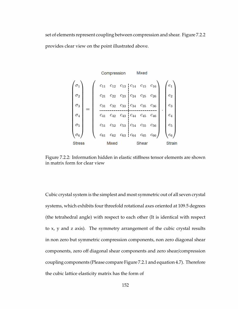
set of elements represent coupling between compression and shear. Figure 7.2.2
provides clear view on the point illustrated above.
Figure 7.2.2: Information hidden in elastic stiffness tensor elements are shownin matrix form for clear view
Cubic crystal system is the simplest and most symmetric out of all seven crystal
systems, which exhibits four threefold rotational axes oriented at 109.5 degrees
(the tetrahedral angle) with respect to each other (It is identical with respect
to x, y and z axis). The symmetry arrangement of the cubic crystal results
in non zero but symmetric compression components, non zero diagonal shear
components, zero off diagonal shear components and zero shear/compression
coupling components (Please compare Figure 7.2.1 and equation 4.7). Therefore
the cubic lattice elasticity matrix has the form of
152

σ1
σ2
σ3
σ4
σ5
σ6
=
c11c12c12 0 0 0
c12c11c12 0 0 0
c12c12c11 0 0 0
0 0 0 c44 0 0
0 0 0 0 c44 0
0 0 0 0 0 c44
.
e1
e2
e3
e4
e5
e6
(7.2.7)
Elastic constants (ci j) play an important roles in solids since it is directly re-
lated to inter-atomic bond rigidity hence the inter atomic potentials. Fur-
thermore elastic properties such as Bulk modulus(B), Poisson ratio(ν), Zener
anisotropy(A), Shear modulus (G) etc. can be easily determined by using
elastic constants. Bulk modulus is simply the ratio of pressure applied from
all direction in to the solid to the fractional change in the volume of the
solid(∆P/(∆V/V)). In simple words it implies the pressure(usually measured in
GPa) which needs to be applied in order to reduce the volume of the materials
by 100% or its the measure of the ability of a substance to withstand changes in
volume when under compression on all sides. The reciprocal of bulk modulus
is known as ”compressibility” and is not only a property of solids but also liq-
uids and gasses. In cubic structures bulk modulus is related to elastic constants
such that B = (C11 + 2C12)/3.
Crystals anisotropy can be determined using Zener anisotropy constant which
is a dimensionless constant. For cubic crystal it is related to elastic constants
153

by A = 2C44/(C11 − C12). Poisson’s ratio is the ratio of transverse contrac-
tion strain to longitudinal extension strain in the direction of stretching force
(ν = −etransverse/elongitudinal). Tensile deformation is considered positive and com-
pressive deformation is considered negative. The definition of Poisson’s ratio
contains a minus sign so that normal materials have a positive ratio. For
isotropic crystals the Poisson’s ratio can be determined by using the equation
A = (3B − 2G)/(6B + 2G) where G denotes the shear modulus of the crystal.
In practical perspectives Poisson’s ratio compares the strength or resistance of
the material against deformation in lateral and longitudinal axes of different
materials. As an example Copper(ν = 0.35)[192] resists lateral deformation
more effectively than natural rubber(ν = 0.4999) [192].
7.3 Resonant ultrasound spectroscopy fundamentals
Couple of most conventional methods used to measure elastic properties of
solids are pulse-echo techniques and continuous-wave method. It is important
to understand that the key feature to both of these methods is plane wave
propagation. Time of flight of plane wave propagated through the sample
held in between two piezoelectric transducers along with the sample thickness
and correction to transducer effects are used to measure the ultrasonic sound
velocity.
154

Figure 7.3.1: Typical setup used for RUS measurements
RUS offers an approach which differs fundamentally from the more conven-
tional methods just described. RUS does not rely on the plane-wave approxi-
mation; indeed there are no plane waves. Instead, RUS is based on the measure-
ment of the vibrational eigenmodes of samples of well defined shapes, usually
parallelepipeds or spheres. A typical experimental arrangement is illustrated
in Figure 7.4.1. A parallelepiped shaped sample is held by two piezoelectric
transducers. One of the transducer excites the samples with range of frequen-
cies corresponding to a large number of vibrational eigenmodes of the sample.
The opposite transducer receives the resonant response of the sample. Once
the transducer frequency matches with an eigenfrequency of the sample a large
response(signal) can be observed. The eigenfrequencies depend on the elastic
constants, the sample shape, the orientation of the crystallographic axis with
respect to the sample, and the material density. By measuring a large num-
ber of resonant frequencies on one sample it is possible to obtain information
155
about all of these quantities. (The square of the frequencies depends on the
product of the elastic constants and the linear dimensions of the sample; thus,
elastic constants and linear dimensions cannot be determined independently.)
Usually the sample shape, crystallographic orientation, and density are known
and one can determine the complete elastic constant matrix from such a spec-
trum. There is no need to prepare a different sample with different crystalline
orientations. It is apparent that RUS overcomes many of the deficiencies of
more conventional methods used to measure elastic constants.
It is even possible to use samples of dimensions 1 mm. Since there is no plane
wave approximation there are no diffraction effects to worry about. A very
low contact force is being used between the transducer and the sample with
the availability of sensitive electronics. The absence of a bond is very useful for
temperature dependent measurements because differential thermal contraction
often leads to bonds breaking, or at best strains being applied to the sample
under investigation. Further it is far more important near phase transitions.
One good spectrum is more than enough to determine all the elastic constants
hence no need to prepare material in different crystalline direction. This would
help in measuring even low symmetry samples.
7.4 ScF3 sample and RUS setup used
In order to study elastic properties of ScF3 by determining its elastic moduli, an
RUS experiment was performed in Los Alamos National Laboratory under the
156

supervision of Albert Migliori and Boris Maiorov. Albert Migliori is a leading
expert in the use of RUS as a solid state tool and is responsible for developing
the previous versions of similar measurement techniques into so called ”RUS”
technique by expanding the limits in terms of loading and low level electronics.
Figure 7.4.1: (a) Single crystal ScF3 used for RUS measurement. This is thesecond shipment of crystal received from Vladimir Voronov. (b) Experimentalsetup used in Los Alamos National Laboratory
As is mentioned above parallelepiped shape is very common and more impor-
tantly very easy to work with, in RUS measurement. We discussed about this
with our collaborator who prepares samples and were very lucky to receive
a parallelepiped crystal with dimensions 4.7 mm × 3.59 mm × 4.24 mm (Fig-
ure ??). Since it could be little tedious to work with small sample sizes, we
believed our crystal would be an ideal one for RUS measurements in terms of
both size and the shape. The RUS spectra were collected between 300 kHz and
800 kHz using parallelepiped shaped single crystal ScF3 of mass 0.1791 g and
157

density 2.503 g/cm3. Helium flow cryostat was used and minimum of 7 K was
achieved.
7.5 RUS measurement on ScF3
Typical examples of RUS signal are shwon in Figure 7.5.1 and Figure 7.5.2. The
amplitude of the resonance signal as measured by one transducer against the
driving frequancy of the other transducer is recorded and when the sample or
the object in between two transducers is resonating with the driving frequency
a peak or a pulse appears as shown. The corresponding frequency is identified
as the ”resonance frequency”. Figures 7.5.1 and 7.5.2 shows measurements
taken on ScF3 at two different temperatures and it is clearly visible that the
resonance frequency is shifted towards higher values as the temperature is
lowered.
The variation of two resonance frequencies around 360 kHz and 775 kHz were
measured as the temperatures is lowered down to 7 K. Both resonances re-
sponded in a similar manner as shown in Figures 7.5.3 and 7.5.4. Towards the
lower end of temperatures a sharp increase in frequency could be observed.
The red line indicates how the line width (Gamma) of the resonance signal
varies against the temperature.
The line width of the resonance signal is proportional to the dissipation of
ultrasonic energy caused by dynamic fluctuations such as vibrations in the
system. Below ∼ 40 K drastic increase in resonance line width and sharp
158

5 2 0 5 3 0 5 4 0 5 5 0
- 0 . 0 5
0 . 0 0
0 . 0 5
Trans
duce
r Res
pons
e [V]
F r e q u e n c y [ k H z ]
3 0 3 K 2 9 8 K
Figure 7.5.1: Typical example of RUS signal. Two sharp peaks indicate reso-nance vibrations of ScF3 lattice around 500 kHz
5 9 0 5 9 5 6 0 0 6 0 5- 0 . 0 3
- 0 . 0 2
- 0 . 0 1
0 . 0 0
0 . 0 1
0 . 0 2
0 . 0 3
Trans
duce
r Res
pons
e [V]
F r e q u e n c y [ k H z ]
3 0 3 K 2 9 8 K
Figure 7.5.2: Resonance vibrations around 600 kHz
159

increases in resonance frequency are observed, revealing that some source
of energy dissipation is activated in the system at ∼ 40 K. This was neither
a straight forward nor an expected result for this material therefore could
be very challenging to interpret. Apart from the above observations if we
closely observe the line width variation in both spectra, a clear indication of
discontinuity can be observed in the temperature window of 75 - 100 K. It
is intriguing that we have already discussed the same temperature range in
the context of central peak appearance, the thermal expansion saturation and
extrapolated temperatures for disordered ScF3 systems in section 2.3.7, 2.3.3
and 2.3.11 respectively.
In an attempt to understand our results it is worthwhile to compare them with
previous results obtained using similar techniques and systems.
Almost identical behavior of resonance line width was previously observed in
SrTiO3[193] and it is clearly visible below ∼ 105 K, the temperature at which it
breaks its cubic symmetry to tetragonal, a well known ferroelastic transition.
The variation of the line width was explained with connection to mobile twin
wall formation and common among most of the ferroelastic materials. In
fact for SrTiO3 highly mobile ferroelastic twin walls in tetragonal phase was
proposed by Kityk et al. [194] even before. Apart from notable increase in
dissipation in energy Scott et al. have observed [193] an abrupt fall is resonance
frequencies below 105 K transition. Both of these features were attributed to
the increase in number density of domain walls and their mobility(damping).
160
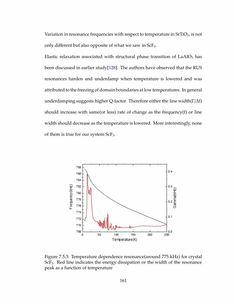
Variation in resonance frequencies with respect to temperature in SrTiO3, is not
only different but also opposite of what we saw in ScF3.
Elastic relaxation associated with structural phase transition of LaAlO3 has
been discussed in earlier study[128]. The authors have observed that the RUS
resonances harden and underdamp when temperature is lowered and was
attributed to the freezing of domain boundaries at low temperatures. In general
underdamping suggests higher Q-factor. Therefore either the line width(Γ/∆f)
should increase with same(or less) rate of change as the frequency(f) or line
width should decrease as the temperature is lowered. More interestingly, none
of them is true for our system ScF3.
Figure 7.5.3: Temperature dependence resonance(around 775 kHz) for crystalScF3. Red line indicates the energy dissipation or the width of the resonancepeak as a function of temperature
161

Figure 7.5.4: Temperature dependence resonance(around 380 kHz) for crystalScF3. Red line indicates the energy dissipation or the width of the resonancepeak as a function of temperature
Soft modes(acoustic or optic) coupled with acoustic phonon modes is com-
mon among perovskites associated phase transition and almost all of them
are known to be displacive phase transitions. Appearance of elastic or quasi-
elastic peak near the phase transition temperature was first observed in 1971
by Riste(Please refer chapter 1 for more details) by performing a neutron scat-
tering experiment which is known as the central peak and was thoroughly
discussed in Chapter 2. In general the relaxation time for the central peak
mode indicates 110 MHz. As an example for LaAlO3 central peak has the time
scale of 20 ns[128]. One of the theory proposes that central peak could emerge
from a combination of phonon density fluctuations and flipping of clusters of
162
tilted octahedra between different 〈111〉, 〈011〉 and 〈001〉 axes [128]. Further
studies have shown that in the corresponding temperature interval the twin
wall widths become wider[195] and a variety of other anomalies appear in the
evolution of strain parameters and optic phonon frequencies [196].
ZrW2O8[136] elastic constants C11, C12 and C44 gets harden as the temperature
decreases. This infers that the material gets stiffer as the temperature is lowered
which is consistent with the results obtained for similar type material ScF3.
In contrast ScF3 predicts more sensitive elasticity behavior, in the context of
approaching to quantum phase transition.
We have not yet carried out the full analysis of refining temperature dependent
elastic constants Ci j’s of ScF3. It will be carried out as next phase of the same
project and demands advanced computer simulations. Once it will be taken
care of I would expect that the role of elasticity on the instability of incipient
ferroelastic modes of ScF3 as it approaches to quantum phase transition would
unravel.
163

Chapter 8
Instrumentation Development
8.1 Introduction
materials and their significant properties are well understood by studying their
electron system and their basic structure. By far physics has mostly contributed
to unravel mysteries behind new phenomenon of these materials. Even though
the invention of the transistor happens in 1947 [197], the first ever semicon-
ductor effect was observed by Michael Faraday in 1833 [198] and since then
material science has come a long way and it still is uncovering new mate-
rial types. Some of them have the potential to be the future of humankind
perhaps in near future or 100s of years from now. In order to understand
materials behavior we need to understand the fundamentals through their
electron arrangement or the structure. As an example almost all the properties
of semiconductors are well understood and very well explained in terms of
theory (simple one-electron theories such as the local-density approximation
(LDA) of density-functional theory or Hartree-Fock theory) and they have been
developed up to an optimum level that they could be useful in terms of exper-
iment. We know semiconductors are relatively simple electron systems since
164
the valence states involve incompletely filled s or p electron shells. There are
other classes of materials which have partially filled d or f electron shells, hence
high electron density and the effects of coulomb repulsion are important. We
identify these types of systems as strongly correlated electron systems. Exam-
ples of this category includes high-temperature superconductors, topological
Kondo insulators and Mott insulators. A wide range of condensed matter
researchers are interested in strongly correlated systems since they display of
very interesting properties. Out of various sorts of experimental techniques,
one of the most used and succeeded techniques to investigate them is to study
the optical properties at different frequencies as temperature is varied. Ex-
amples of such properties are optical conductivity σ(ω), refractive index n(ω),
dielectric constant n(ω) etc. Optical properties are very important to study fun-
damental materials properties such as energy band structure, impurity levels,
excitons, localized defects, lattice vibrations, and certain magnetic excitations.
As an example the frequency-dependent complex dielectric function ε(ω) or
the complex conductivity σ(ω) is directly related to the energy band structure
of solids. For semiconductors, the core dielectric constant ε0 is typically a
large number and the contribution due to the free carriers is small at infrared
and visible frequencies. For metals, the free carrier absorption is dominant
over the entire optical frequency range. Another example is that the impu-
rity spectra are studied most directly by infrared absorption and transmission
measurements. Even the optical lattice modes at q = 0 are sensitively probed
165

by infrared spectroscopy, which we have applied to study ScF3 and already
discussed in Chapter 6.
8.2 Fourier Transformed Infrared Spectrometer
We designed and developed an instrumentation in order to carry out optical
measurements, which would cover broad frequency range (1 cm−1 < ω < 10000
cm−1) and wide temperature (4 K<T<400 K) range. Development of the in-
strumentation was carried out in the laboratory at the Department of Physics,
University of Connecticut. A Bruker 70v Fourier Transformed Infrared (FTIR)
spectrometer and a combination of photovoltaic and bolometer detectors cover
frequencies of 150 cm−1 < ω < 10000 cm −1. In order to focus the beam from
FTIR to the sample and then to the detector we designed an optical layout con-
sists of off-axis aspherical mirrors. More importantly we invented a method to
construct low-cost aspherical mirrors which were then installed in the mirror
layout.
166
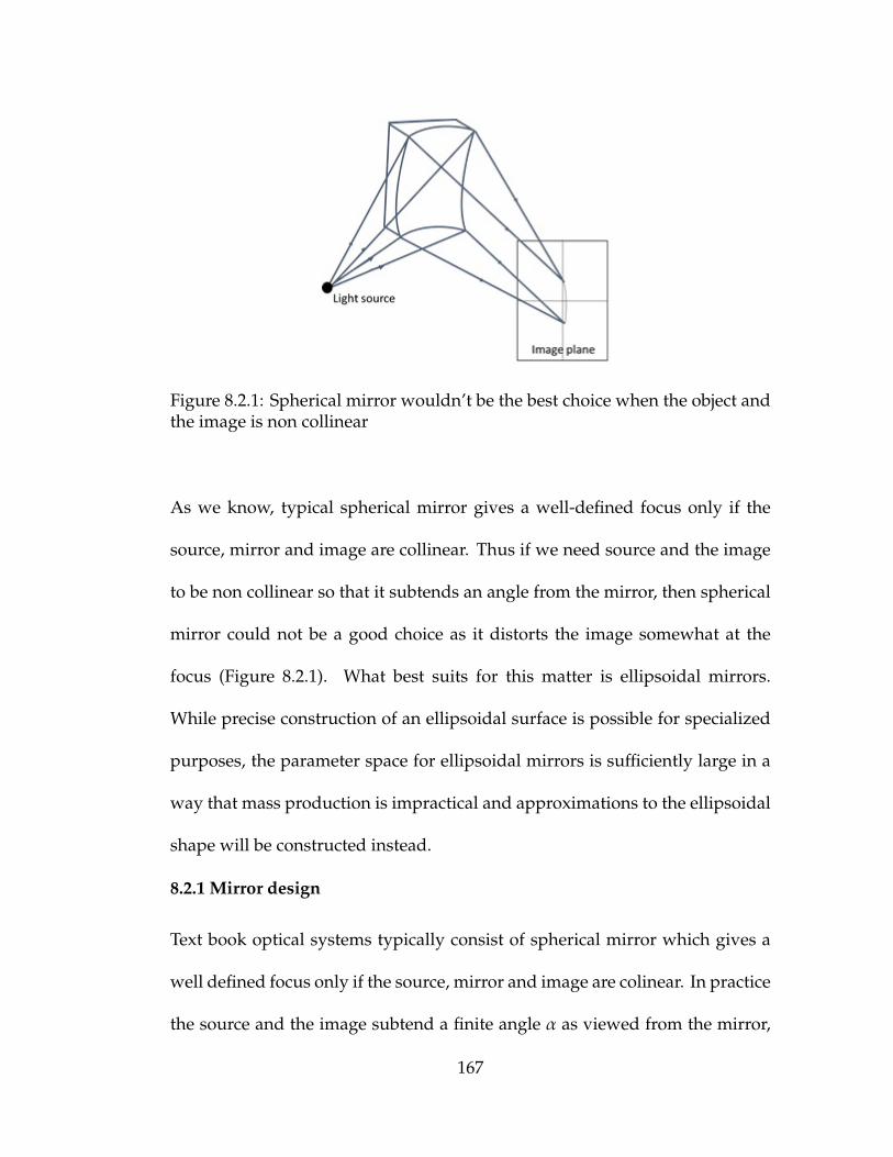
Figure 8.2.1: Spherical mirror wouldn’t be the best choice when the object andthe image is non collinear
As we know, typical spherical mirror gives a well-defined focus only if the
source, mirror and image are collinear. Thus if we need source and the image
to be non collinear so that it subtends an angle from the mirror, then spherical
mirror could not be a good choice as it distorts the image somewhat at the
focus (Figure 8.2.1). What best suits for this matter is ellipsoidal mirrors.
While precise construction of an ellipsoidal surface is possible for specialized
purposes, the parameter space for ellipsoidal mirrors is sufficiently large in a
way that mass production is impractical and approximations to the ellipsoidal
shape will be constructed instead.
8.2.1 Mirror design
Text book optical systems typically consist of spherical mirror which gives a
well defined focus only if the source, mirror and image are colinear. In practice
the source and the image subtend a finite angle α as viewed from the mirror,
167

distorting the fidelity of the mirror as an image component. Here we show
how to construct aspheric mirrors from low-cost prescription lenses.
Aspheric corrections to the mirror shape can accommodate off-axis optical
arrangements. Optical design can be limited by available components. We
consider the general problem of focusing a source at a distance s to an image at
a distance t with incident angle α. The ideal mirror shape which accomplishes
this goal is a part of a prolate ellipsoid. Prolate ellipsoid of revolution is
x2
a2 +y2 + z2
b2 = 1 (8.2.1)
with a>b=c.
If a source of light is placed at (d, 0, 0) then the emitted light will traverse
the same distance from the source to any point on the mirror, to the other
focus independently of which surface point it reflects. The prolate ellipsoid is
special, because a spherical wave emitted at one focus, reflected from any point
on the interior surface is sent to the other focus where it arrives with a phase
independent of where the wave front was reflected. Constructive interference
between all pathway guarantees a crisp tight focus in this ideal case. Any
segment of the full prolate ellipsoid would then constitute an ideal optical
element for our purpose.
Figure 8.2.3 shows the prolate ellipsoid with two planes of interests. Due to
the cylindrical symmetry first consider the plane y = 0. The intersection of
168
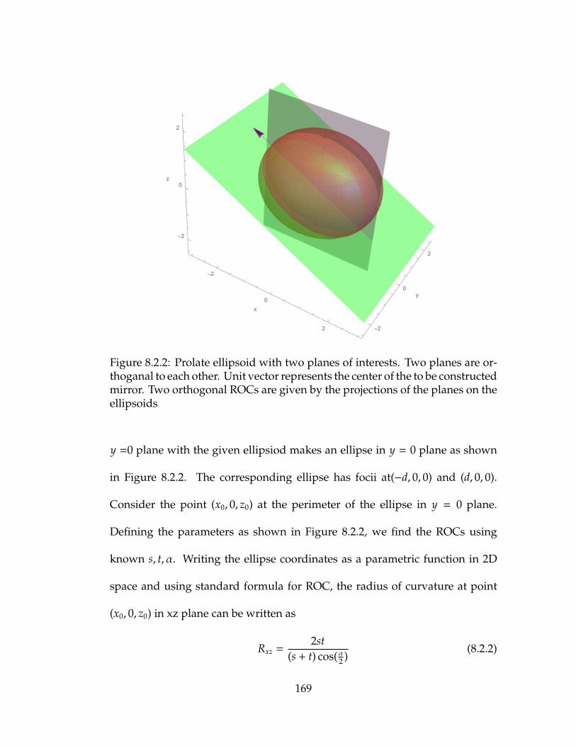
Figure 8.2.2: Prolate ellipsoid with two planes of interests. Two planes are or-thoganal to each other. Unit vector represents the center of the to be constructedmirror. Two orthogonal ROCs are given by the projections of the planes on theellipsoids
y =0 plane with the given ellipsiod makes an ellipse in y = 0 plane as shown
in Figure 8.2.2. The corresponding ellipse has focii at(−d, 0, 0) and (d, 0, 0).
Consider the point (x0, 0, z0) at the perimeter of the ellipse in y = 0 plane.
Defining the parameters as shown in Figure 8.2.2, we find the ROCs using
known s, t, α. Writing the ellipse coordinates as a parametric function in 2D
space and using standard formula for ROC, the radius of curvature at point
(x0, 0, z0) in xz plane can be written as
Rxz =2st
(s + t) cos(α2 )(8.2.2)
169

Figure 8.2.3: Prolate ellipsoid with focii at(−d, 0, 0) and (d, 0, 0). (x0, 0, z0) de-notes the center position of the to be constructed mirror with specificationss, t and α. They denote the object distance, image distance and the angle inbetween respectively.
In order to solve for the ROC, orthogonal to Rxz we now consider the more
difficult case in which the ROC lies in a plane perpendicular to the y = 0 plane
To achieve this, lets do a simple coordinate transformation such that the z axis
of the new coordinate system (z′) is in parallel with the normal vector as shown
in Figure 8.2.3. Lets the plane of interest be y′z′ and the ROC at point (x0, 0, z0)
in y′z′ plane can be found as (Please see Appendix ?? for detailed calculations.)
Ry′z′ =2stcos(α/2)
(s + t)(8.2.3)
Likewise the two orthogonal ROCs are found at a point in an ellipsoidal surface
and should correspond to an arbitrary toroidal surface. Therefore we have
170
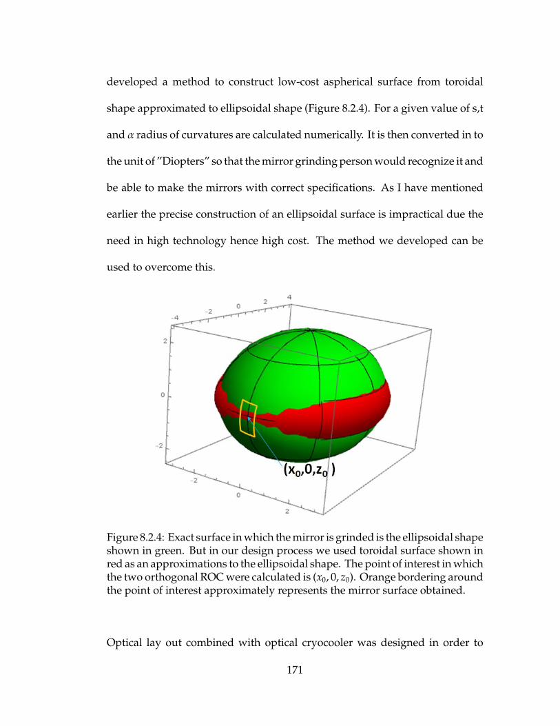
developed a method to construct low-cost aspherical surface from toroidal
shape approximated to ellipsoidal shape (Figure 8.2.4). For a given value of s,t
and α radius of curvatures are calculated numerically. It is then converted in to
the unit of ”Diopters” so that the mirror grinding person would recognize it and
be able to make the mirrors with correct specifications. As I have mentioned
earlier the precise construction of an ellipsoidal surface is impractical due the
need in high technology hence high cost. The method we developed can be
used to overcome this.
Figure 8.2.4: Exact surface in which the mirror is grinded is the ellipsoidal shapeshown in green. But in our design process we used toroidal surface shown inred as an approximations to the ellipsoidal shape. The point of interest in whichthe two orthogonal ROC were calculated is (x0, 0, z0). Orange bordering aroundthe point of interest approximately represents the mirror surface obtained.
Optical lay out combined with optical cryocooler was designed in order to
171

perform IR reflectively and transmission spectroscopy. Selected parameters
for mirrors in optical lay out are given in Table 8.1. The corresponding mirror
layout is shown in Figure 8.2.5.
Figure 8.2.5: Optical layout combined with cryocooler. Specifications of eachmirrors are given in Table 6.1. Gray colored mirrors are plane mirrors and thewhole layout can be rotated around them. A sharp aperture is placed at thefocus of M0 mirror. This defines the object to M1 mirror which forms an imageat the sample space. Light reflects from and transmits through the sample arecollected by M2r and M2t mirrors and refocused into detectors(Red colored) byM3r and M3t mirrors
8.2.2 Vibration-free, cryogen-free optical cryocooler
172

Mirror name Incident angle Object distance, Image distance(α) in inches(s) in inches(t)
————————-———————– ———————— ——————–M0 25o
∞ 9M1 30o 9 9M2r 30o 9 ∞
M2t 30o 9 ∞
M3r 40o∞ 6
M3t 40o∞ 6
Table 8.2.7: Specifications of mirrors used in mirror layout shown in Figure8.2.5. Here ∞ means the beam is parallel. The mirror notation is used foridentification purpose.
One of the main instrumentational project in the laboratory is combining optical
layout with vibration-free, cryogen-free optical cryocooler for low temperature
optical measurements. In order to achieve this, one of the chamber of cryo-
stat had to be modified, so that it can be used for low temperature optical
measurements. To accomplish this, several parts were custom made with the
help of machine shop engineer in Physics. These parts, combining with spher-
ical square from Kimball Physics, feed through rod from MDC vacuum and
translational stage from Newport were assembled together. One of the main
consideration, to reduce the temperature difference between the cold finger of
the cryostat (at the center) and the sample holder is, how to minimize the heat
gain by the sample holder in form of radiation from outside. This was achieved
by a custom made radiation shield, consists of three pieces made of Aluminum.
8.3 Time-Domain Terahertz(TD- THz) spectrometer
We built a TD- THz spectrometer as our next phase of instrumentation. THz will
173

Figure 8.2.6: Custom made components for optical cryocooler.
cover the frequency range of 1 cm−1 < ω < 1150 cm−1 and this spectrometer con-
sists of several apparatus (Figure 8.3.2) such as KMLabs Griffin -10 Ti:Sapphire
pulsed laser, photoconductive THz emitter, high precision linear stage delay
line. The laser has the ability to produce femtosecond pulses(transform limited
of 10 fs) at 95 MHz repetition rate. Incoming laser pulses were compressed and
split into two beams, high intense (greater than 200 mW but less than 600 mW)
laser beam (pump beam) burst in to photoconductive THz emitter in order to
174
generate THz and the less intense probe laser beam was used for detection of
THz.
8.3.1 Introductory to TD-THz spectrometer
Terahertz spectroscopy is a technique which is utilized to measure physical
phenomena within the time scale of sub picoseconds. While THz systems
are used in both spectroscopic and imaging applications the generation and
detection of THz radiation is performed using pump-probe approach. The
first THz generation was achieved in late 70s by studying the response of
photoconductors to laser pulses. In the late 80s, the first practical pulsed THz
system was invented and photoconductive antennas was used to generate and
detect THz radiation. The other well-known method to generate THz radiation
is the non linear optical phenomenon known as second harmonic generation.
Subfemtosecond laser pulses burst in to non linear electro-optic crystals are
capable of generating THz radiation of high frequency which is not possible
with photoconductinve antenna arrays.
175

Figure 8.3.1: THz frequency range with respect to the whole electromagnticspectrum. The range approximately is in between 2 meV and 20 meV.
Laser pulses are used to generate and detect THz and this is usually done
by splitting the laser pulses into two beams which are identified as pump
beam and probe beam. Typical laser pulse duration would be 10 to 120 fs and
in most cases the pump beam is higher in energy than the probe beam and
is capable of generating electromagnetic transient through career excitation
of a photoconductive antenna or electro-optic crystal. The electromagnetic
transient which is in the range of few ps corresponds to THz wave. In order to
detect THz wave, one of the beam is delayed, in most cases by using mechanical
delay line. The THz E-field would be measured as a function of time difference
between the pump and the probe beam. The THz detection is carried out either
by using the inverse process of the generation achieved by photoconductive
antenna or by using electro-optic effect with the aid of electro-optic crystals.
Compare with other spectroscopic techniques THz has its own differences.
When we utilize FTIR or Raman spectroscopy, the signal is directly proportional
176

to the intensity or in other words we measure the number of photons which
we detect at each frequency, (|E(ω)|2). In contrast, with THz spectroscopy we
obtain the time dependent electric field (E(t)) which measures not only the
photon energy but also when the photon arrives to the detector. As a result
the measured signal contains the information about both the amplitude and
phase of the THz wave. This allows to calculate both real and imaginary part
of dielectric constants of a material in a straight forward way compared with
FTIR, in which we have to use Kramers-Kronig(KK) transformation to obtain
corresponding quantities. As an example if we measure the THz transmission
of a sample, then the ratio of Fourier transformation of sample signal(time
domain THz signal) to Fourier transformation of reference signal gives the
complex transmission of the sample with respect to the reference. Since the
complex transmission is related to complex refractive index (not in a trivial
way but can be solved analytically) an iterative method of calculation can be
used to solve for refractive index hence dielectric function. But in case of IR
spectroscopy, we calculate the power ratio of raw signal of sample to reference
signal as the reflectance and hence obtain only the real part of refractive index.
In order to find imaginary part we have to use KK transformation.
Another distinct advantageous of THz spectroscopy is that its capability of
probing soft phonons. FTIR can also be utilized for low frequency( above 60
µm wavelength or less than 5 THz) measurements but the detection has to
be carried out using Bolometers which require liquid Helium to operate with,
177

therefore the data collection is much harder and expensive. In addition the
FTIR signal has low signal to noise ratio compared with THz signal in the same
frequency range.
It is also worthwhile to mention that THz signal can be used as fingerprints to
identify many molecules, especially most of the organic polymers have unique
absorption features at THz frequency. Apart from that THz can see through
most of the non metallic materials which are opaque to optics. Even thin(∼ nm
or 10 µm) metallic samples are probed with THz in order to determine their
carrier concentration, due to the absorption arises from free carriers.
8.3.2 Our TD-THz spectrometer
The femtosecond laser pulse is separated into the probe and pump beams. The
energy of the pump beam is about 700 mw and the energy of the probe beam
is about 100 mW. The laser beam is split using a polarized beam splitter. laser
pulse is linearly polarized and the beam splitter decomposes the polarization
of the beam in two perpendicular components. One of the components will
be the pump beam while the other perpendicular component will be the probe
beam. A half wave plate is used before the beam splitter such that by changing
the polarization angle the amount of energy for each component is controlled
thus, the energy ratio between pump and probe pulses can be adjusted. A
mechanical delay line is introduced in pump beam path and the maximum
translation is 150 mm which corresponds to ∼ 1 ns. The THz radiation is
178

generated by biased photonconductive antenna(or arrays of antennas) excited
by pump laser beam. Main feature of an antenna is the gaped metal electrodes
which are deposited on a semiconductor substrate. The pump beam excites the
gap which leads to the generation of photocarriers. The free carriers are then
accelerated by an external bias voltage and the accelerated electrons produce
THz radiation.
Figure 8.3.2: Current THz spectrometer.
Generated THz pulse focuses into sample and refocuses into a detection crystal
ZnTe (using set of off-axis parabolic mirrors of focal lengths of 4 inches), where
it meets with the probe beam. The THz spot and the probe laser spot should
overlap on the detection crystal in order to achieve maximum efficiency. So the
output signal is typically proportional to the convolution of the probe beam
and the THz pulse. The output signal is detected using lock-in detection as
one has to detect very small changes in polarization in the probe beam or very
low signal compared with the noise (very low signal to noise ratio(SNR)). In
179
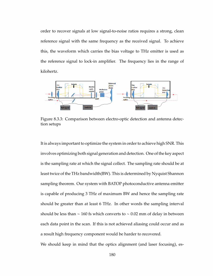
order to recover signals at low signal-to-noise ratios requires a strong, clean
reference signal with the same frequency as the received signal. To achieve
this, the waveform which carries the bias voltage to THz emitter is used as
the reference signal to lock-in amplifier. The frequency lies in the range of
kilohertz.
Figure 8.3.3: Comparison between electro-optic detection and antenna detec-tion setups
It is always important to optimize the system in order to achieve high SNR. This
involves optimizing both signal generation and detection. One of the key aspect
is the sampling rate at which the signal collect. The sampling rate should be at
least twice of the THz bandwidth(BW). This is determined by Nyquist Shannon
sampling theorem. Our system with BATOP photoconductive antenna emitter
is capable of producing 3 THz of maximum BW and hence the sampling rate
should be greater than at least 6 THz. In other words the sampling interval
should be less than ∼ 160 fs which converts to ∼ 0.02 mm of delay in between
each data point in the scan. If this is not achieved aliasing could occur and as
a result high frequency component would be harder to recovered.
We should keep in mind that the optics alignment (and laser focusing), es-
180
pecially with four off-axis parabolic mirrors is key when the high frequency
component of the THz signal is detected. If PCA array is used for detection
(Please refer Figure 8.3.3 to understand the differences of the set ups from EO
detection), the accurate alignment becomes more critical. In order to achieve
this we need to match the laser beans at both the emitter and detector ends.
This can be done by removing the antennas from the setup and guiding the
emitter beam through THz optics(parabolic mirrors) to the last mirror before
the detector position. Then we need to repeat it for the detector laser beam
till it reaches the last mirror before the emitter position. Both beams should
be coincident on both end mirrors. We use iris diaphragms or an IR viewer to
confirm it. After this step we know that both beams are completely collinear
through our setup. Then we integrate our antennas into the setup.
When we put back the antennas we have to make sure that the position of
the antenna with respect to the optical beam is correct such away that a good
illumination is assured. Additionally we have to put the antenna at the correct
distance from the first parabolic mirror.
The virtual source point should be in the focal distance of the parabolic mirror.
The virtual source point for the BATOP antenna is roughly 18.7 mm behind the
antenna chip(Figure8.3.4 ). Then we perform a THz scan and find the delay
line position corresponds to the signal peak. After that we move the delay
line to the maximum signal position and optimize the THz signal. Now we
believe that the antennas should be illuminated fine and we concentrate on
181

the alignment of the THz part. We tilt the mirrors until we get the maximum
signal strength and the maximum THz bandwidth also should be achieved at
the same delay position. We confirm the position of the delay line from time
to time, as the THz beam path length can be changed a bit in the process of
adjusting the parabolic mirrors.
Figure 8.3.4: The virtual source point for the BATOP antenna is roughly = L -d = 18.7 mm behind the antenna chip
The SNR can always be increased by averaging. If the number of collec-
tions(sampling) at a given delay (at a single data point) can be increased,
higher SNR can be achieved but with longer total scan time duration. So it is
always pivotal to decide the optimum numbers of sampling to average when
data is collected.
Frequency resolution is very important when spectra are collected. If we
182
want to study features which our instrument is not capable of resolving, that
is pointless. So the resolution that the spectrometer can deliver is always
critical. Frequency resolution depends on scan range of a particular scan. As
an example if we require to observe a narrow absorption peak of 1 GHz, then
we need to achieve minimum of 1 GHz resolution which corresponds to 1
ns of delay. That is the maximum delay we could achieve with our system
therefore the maximum resolution as well. On the other hand if we want to
study features of 100 GHz wide, then the related delay is only 10 ps or about
couple of millimeters.
THz radiation is very sensitive to atmosphere. Water and CO2 molecules
in atmosphere result in strong wiggles in time domain signal which is then
interpreted as sharp absorption features in frequency domain. The frequencies
of such features correspond to different vibrational modes of the molecules.
This can be overcome by purging instrument with dry Nitrogen air.
It is also important to realize that 0.3 THz wave has wavelength of 1 mm. The
theoretical limit of focus or diffraction limited spot diameter at sample at this
wavelength is about 2 mm (using ∼ Fλ/D, where the focal length of parabolic
mirror, F is 4 inches and the diameter of parabolic mirror,D is 2 inches.) If we
are to use samples with similar dimensions we approach the diffraction limit
hence we always have to incorporate a low frequency cutoff to spectroscopy. In
order to make sure that long wave lengths(which are longer than the sample)
do not pass around the sample we setup an aperture smaller than the sample
183

and make sure it is very close to the sample surface hence very much near the
focus of the beam. In this case the lower cut off is determined by the aperture
diameter. Another approach is to apply silver glue around the sample.
Photoconductive antenna
We use couple of photoconductive antennas. One of them is large area pho-
toconductive antenna known as Tera-SED from Laser Quantum and the other
is broad area interdigital photoconductive THz antenna with micro lens array
and hyperhemispherical silicon lens from BATOP optoelectronics [199].
The laser beam must be collimated at the position of the antenna. The optimum
laser beam diameter must be found. The minimum optical power per illumi-
nated pixel on the antenna is about 1 mW. The hexagonal pitch is 30 um. The
illuminated diameter for 100 pixels is therefore about 300 um for 1mW/pixel. I
propose to use a laser beam diameter of about 200 um at first. Since we do not
have a powerful fs laser, we cannot make experiments to find the optimized
power density on such an array antenna. The minimum laser beam diameter
is given by the maximum power of 10 mW per pixel. For 10 pixel (100 mW)
the minimum illuminated diameter would be about 100 um. You may need a
telescope to adjust the collimated laser beam on the antenna to the mentioned
diameter of 200 um.
184

8.3.3 THz signal
Figure 8.3.5: Time Domain THz signal
Figure 8.3.6: Frequency Domain THz signal
185

Appendix A
Construction of an optical system
Figure A.3.7: ellipse shown in xyz coordinate,y is perpendicular to the plane
Equation of an ellipsoid is given by,
x2
a2 +y2 + z2
b2 = 1 (A.3.1)
Consider the plane y = 0 , cuts the given ellipsoid. The equation of the new
ellipse on y= 0 plane is given by,
x2
a2 +z2
b2 = 1 (A.3.2)
186

Where d is the distance from the center to either focus. a and b are transverse
diameter(along x-semi major axis) and conjugate diameter(along z- semi minor
axis) respectively.
Consider a point of the ellipse (x0, 0, z0) and then let us define the distance from
(+d, 0, 0) to (x0, 0, z0) = t, distance from (−d, 0, 0) to (x0, 0, z0) = s and angle made
by (+d, 0, 0),(x0, 0, z0), (−d, 0, 0) =α
Finding unknown using known s, t, α
a =s + t
2(A.3.3)
b =√
a2 − d2 (A.3.4)
d =√
s2 + t2 − 2st cosα (A.3.5)
x0 =t2 + (2d)2
− s2
4d− d (A.3.6)
z0 =ts sinα
2d(A.3.7)
We can write the ellipse as a parametric function in 2D space by defining
x = a cosϑ, z = b sinϑ
The radius of curvature at a certain point(determined by the parameter) is
187
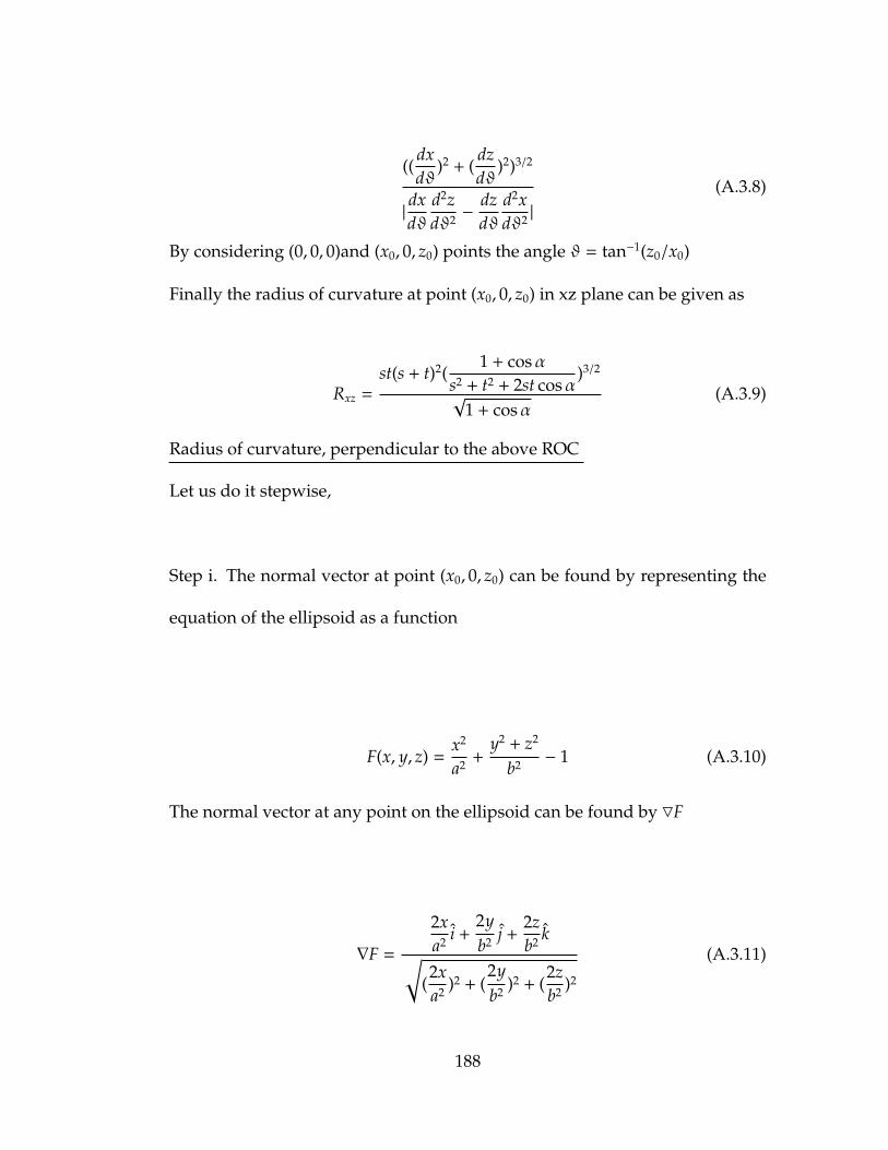
((dxdϑ
)2 + (dzdϑ
)2)3/2
|dxdϑ
d2zdϑ2 −
dzdϑ
d2xdϑ2 |
(A.3.8)
By considering (0, 0, 0)and (x0, 0, z0) points the angle ϑ = tan−1(z0/x0)
Finally the radius of curvature at point (x0, 0, z0) in xz plane can be given as
Rxz =st(s + t)2(
1 + cosαs2 + t2 + 2st cosα
)3/2
√1 + cosα
(A.3.9)
Radius of curvature, perpendicular to the above ROC
Let us do it stepwise,
Step i. The normal vector at point (x0, 0, z0) can be found by representing the
equation of the ellipsoid as a function
F(x, y, z) =x2
a2 +y2 + z2
b2 − 1 (A.3.10)
The normal vector at any point on the ellipsoid can be found by 5F
∇F =
2xa2 i +
2yb2 j +
2zb2 k√
(2xa2 )2 + (
2yb2 )2 + (
2zb2 )2
(A.3.11)
188

The normal vector at point (x0, 0, z0)
∇F =
2x0
a2 i +2z0
b2 k√(2x0
a2 )2 + (2z0
b2 )2
(A.3.12)
Step ii.finding the equation of the normal vector in xz plane
The equation of the normal vector in 2D,which goes through(x0, 0, z0) can be
written as,
(z − z0) = m(x − x0) (A.3.13)
Where m is the gradient and can be found using normal vector
m =z0a2
x0b2 (A.3.14)
The equation of the line becomes
z =( z0a2
x0b2
)x + z0
(1 −
a2
b2
)(A.3.15)
This line cuts z = 0(xaxis) at point x =(−1 +
a2
b2 )
(z0a2
x0b2 )lets take this length as 0L,
where 0L =(−1 +
a2
b2 )
(z0a2
x0b2 )
189
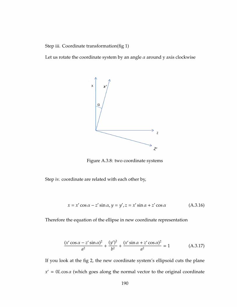
Step iii. Coordinate transformation(fig 1)
Let us rotate the coordinate system by an angle α around y axis clockwise
Figure A.3.8: two coordinate systems
Step iv. coordinate are related with each other by,
x = x′ cosα − z′ sinα, y = y′, z = x′ sinα + z′ cosα (A.3.16)
Therefore the equation of the ellipse in new coordinate representation
(x′ cosα − z′ sinα)2
a2 +(y′)2
b2 +(x′ sinα + z′ cosα)2
a2 = 1 (A.3.17)
If you look at the fig 2, the new coordinate system’s ellipsoid cuts the plane
x′ = 0L cosα (which goes along the normal vector to the original coordinate
190

system’s ellipsoid at point (x0, 0, z0))
Figure A.3.9: ellipse representing in two coordinates
α = tan−1(x0b2
z0a2 ), lookat f ig3 (A.3.18)
By solving the new coordinate system’s ellipsoid at plane x′ = 0L cosα the
equation of the ellipse can be found in new coordinate system
191
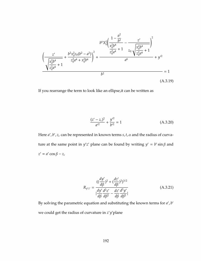
(z′√
x20b4
z20a4
+ 1
+b2x2
0z0(b2− a2)
z20a4 + x2
0b4
)2
+
b6X20
( 1 −a2
b2
x20b4
z20a4
+ 1
−z′
z0
√x2
0b4
z20a4
+ 1
)2
a6 + y′2
b2 = 1
(A.3.19)
If you rearrange the term to look like an ellipse,it can be written as
(z′ − zc)2
a′2+
y′2
b′2= 1 (A.3.20)
Here a′, b′, zc can be represented in known terms s, t, α and the radius of curva-
ture at the same point in y′z′ plane can be found by writing y′ = b′ sin β and
z′ = a′ cos β − zc
Ry′z′ =
((dy′
dβ)2 + (
dz′
dβ)2)3/2
|dy′
dβd2z′
dβ2 −dz′
dβd2y′
dβ2 |
(A.3.21)
By solving the parametric equation and substituting the known terms for a′, b′
we could get the radius of curvature in z′y′plane
192

Ry′z′ =2st cos(α/2)
(s + t)(A.3.22)
193

Bibliography
[1] Jun Chen, Fangfang Wang, Qingzhen Huang, Lei Hu, Xiping Song, JinxiaDeng, Ranbo Yu, and Xianran Xing. Effectively control negative thermalexpansion of single-phase ferroelectrics of pbtio3-(bi, la) feo3 over a giantrange. Scientific reports, 3:2458, 2013.
[2] Xianran Xing, Jinxia Deng, Jun Chen, and Guirong Liu. Novel thermalexpansion of lead titanate. RARE METALS-BEIJING-ENGLISH EDITION,22(4):294–297, 2003.
[3] Masaki Azuma, Wei-tin Chen, Hayato Seki, Michal Czapski, Kengo Oka,Masaichiro Mizumaki, Tetsu Watanuki, Naoki Ishimatsu, Naomi Kawa-mura, Shintaro Ishiwata, et al. Colossal negative thermal expansion inbinio3 induced by intermetallic charge transfer. Nature communications,2:347, 2011.
[4] J Arvanitidis, Konstantinos Papagelis, Serena Margadonna, Kosmas Pras-sides, and Andrew N Fitch. Temperature-induced valence transition andassociated lattice collapse in samarium fulleride. Nature, 425(6958):599–602, 2003.
[5] Brett A Hunter, Brendan J Kennedy, and Tom Vogt. Magnetostriction ina simple trivalent manganese perovskite. Physical Review B, 69(2):020410,2004.
[6] J Rohrkamp, O Heyer, T Fickenscher, R Pottgen, S Jodlauk, H Hartmann,T Lorenz, and JA Mydosh. Thermal expansion of the magnetically or-dering intermetallics rtmg (r= eu, gd and t= ag, au). Journal of Physics:Condensed Matter, 19(48):486204, 2007.
[7] TA Mary, JSO Evans, T Vogt, and AW Sleight. Negative thermal expansionfrom 0.3 to 1050 kelvin in zrw2o8. Science, 272(5258):90, 1996.
[8] Martin T Dove and Hong Fang. Negative thermal expansion and asso-ciated anomalous physical properties: review of the lattice dynamicstheoretical foundation. Reports on Progress in Physics, 79(6):066503, 2016.

[9] Benjamin K Greve, Kenneth L Martin, Peter L Lee, Peter J Chupas,Karena W Chapman, and Angus P Wilkinson. Pronounced negative ther-mal expansion from a simple structure: cubic scf3. Journal of the AmericanChemical Society, 132(44):15496–15498, 2010.
[10] Alfred QR Baron. Introduction to high-resolution inelastic x-ray scatter-ing. arXiv preprint arXiv:1504.01098, 2015.
[11] Jun Chen, Qilong Gao, Andrea Sanson, Xingxing Jiang, Qingzhen Huang,Alberto Carnera, Clara Guglieri Rodriguez, Luca Olivi, Lei Wang, Lei Hu,et al. Tunable thermal expansion in framework materials through redoxintercalation. Nature communications, 8:14441, 2017.
[12] SM Shapiro, JD Axe, G Shirane, and T Riste. Critical neutron scatteringin srti o 3 and kmn f 3. Physical Review B, 6(11):4332, 1972.
[13] JB Hastings, SM Shapiro, and BC Frazer. Central-peak enhancement inhydrogen-reduced srti o 3. Physical Review Letters, 40(4):237, 1978.
[14] T Yagi, H Tanaka, and I Tatsuzaki. Central peak of k h 3 (s e o 3) 2 studiedby light scattering. Physical Review Letters, 38(11):609, 1977.
[15] K Hirota, JP Hill, SM Shapiro, G Shirane, and Y Fujii. Neutron-and x-ray-scattering study of the two length scales in the critical fluctuations ofsrtio 3. Physical Review B, 52(18):13195, 1995.
[16] H-B Neumann, U Rutt, JR Schneider, and G Shirane. Origin of the criticalscattering on two length scales in srtio 3: A high-energy synchrotron-radiation diffraction study. Physical Review B, 52(6):3981, 1995.
[17] T Riste, EJ Samuelsen, K t Otnes, and J Feder. Critical behaviour of srtio3near the 105 k phase transition. Solid state communications, 9(17):1455–1458, 1971.
[18] A Mogus-Milankovic, Jean Ravez, JP Chaminade, and P Hagenmuller.Ferroelastic properties of tf3 compounds (t= ti, v, cr, fe, ga). Materialsresearch bulletin, 20(1):9–17, 1985.
[19] Cody R Morelock, Leighanne C Gallington, and Angus P Wilkinson. Solidsolubility, phase transitions, thermal expansion, and compressibility insc 1- x al x f 3. Journal of Solid State Chemistry, 222:96–102, 2015.
[20] Cody R Morelock, Leighanne C Gallington, and Angus P Wilkinson.Evolution of negative thermal expansion and phase transitions in sc1-xtix f3. Chemistry of Materials, 26(5):1936–1940, 2014.

[21] Cody R Morelock, Matthew R Suchomel, and Angus P Wilkinson. Acautionary tale on the use of ge-7031 varnish: low-temperature thermalexpansion studies of scf3. Journal of Applied Crystallography, 46(3):823–825,2013.
[22] P Daniel, A Bulou, M Rousseau, J Nouet, and M Leblanc. Raman-scattering study of crystallized m f 3 compounds (m= al, cr, ga, v, fe,in): An approach to the short-range-order force constants. Physical Re-view B, 42(16):10545, 1990.
[23] Sahan U Handunkanda, Erin B Curry, Vladimir Voronov, Ayman H Said,Gian G Guzman-Verri, Richard T Brierley, Peter B Littlewood, and Ja-son N Hancock. Large isotropic negative thermal expansion above astructural quantum phase transition. Physical Review B, 92(13):134101,2015.
[24] Ambroise van Roekeghem, Jesus Carrete, and Natalio Mingo. Anomalousthermal conductivity and suppression of negative thermal expansion inscf 3. Physical Review B, 94(2):020303, 2016.
[25] VVSS Sai Sunder, A Halliyal, and AM Umarji. Investigation of tetrago-nal distortion in the pbtio 3–bifeo 3 system by high-temperature x-raydiffraction. Journal of materials research, 10(5):1301–1306, 1995.
[26] SA Mabud and AM Glazer. Lattice parameters and birefringence in pbtio3single crystals. Journal of Applied Crystallography, 12(1):49–53, 1979.
[27] Fangfang Wang, Ying Xie, Jun Chen, Honggang Fu, and Xianran Xing.First-principles study on negative thermal expansion of pbtio3. AppliedPhysics Letters, 103(22):221901, 2013.
[28] Jun Chen, Krishna Nittala, Jennifer S Forrester, Jacob L Jones, Jinxia Deng,Ranbo Yu, and Xianran Xing. The role of spontaneous polarization inthe negative thermal expansion of tetragonal pbtio3-based compounds.Journal of the American Chemical Society, 133(29):11114–11117, 2011.
[29] Yi He. Heat capacity, thermal conductivity, and thermal expansion ofbarium titanate-based ceramics. Thermochimica acta, 419(1):135–141, 2004.
[30] JS Forrester, EH Kisi, KS Knight, and CJ Howard. Rhombohedral tocubic phase transition in the relaxor ferroelectric pzn. Journal of Physics:Condensed Matter, 18(19):L233, 2006.
[31] MS Senn, A Bombardi, CA Murray, C Vecchini, A Scherillo, X Luo, andSW Cheong. Negative thermal expansion in hybrid improper ferroelectricruddlesden-popper perovskites by symmetry trapping. Physical reviewletters, 114(3):035701, 2015.
[32] Yangchun Rong, Menglei Li, Jun Chen, Mei Zhou, Kun Lin, Lei Hu,Wenxia Yuan, Wenhui Duan, Jinxia Deng, and Xianran Xing. Large neg-ative thermal expansion in non-perovskite lead-free ferroelectric sn 2 p 2s 6. Physical Chemistry Chemical Physics, 18(8):6247–6251, 2016.
[33] Ikuya Yamada, Kazuki Tsuchida, Kenya Ohgushi, Naoaki Hayashi, JungeunKim, Naruki Tsuji, Ryoji Takahashi, Masafumi Matsushita, NorimasaNishiyama, Toru Inoue, et al. Giant negative thermal expansion in the ironperovskite srcu3fe4o12. Angewandte Chemie International Edition, 50(29):6579–6582, 2011.
[34] YW Long, N Hayashi, T Saito, M Azuma, S Muranaka, and Y Shimakawa.Temperature-induced a–b intersite charge transfer in an a-site-orderedlacu3fe4o12 perovskite. Nature, 458(7234):60–63, 2009.
[35] CH Xu, CZ Wang, Che Ting Chan, and KM Ho. Theory of the thermalexpansion of si and diamond. Physical review B, 43(6):5024, 1991.
[36] M Leszczynski, VB Pluzhnikov, A Czopnik, J Bak-Misiuk, and T Slupin-ski. Thermal expansion of gaas: Te and algaas: Te at low temperatures.Journal of applied physics, 82(9):4678–4680, 1997.
[37] NV Anshukova, BM Bulychev, AI Golovashkin, LI Ivanova, IB Krynet-skii, AA Minakov, and AP Rusakov. Anomalous low-temperature be-havior of the thermal characteristics of mgb2. Journal of Experimental andTheoretical Physics, 97(1):70–77, 2003.
[38] JJ Neumeier, T Tomita, M Debessai, JS Schilling, PW Barnes, DG Hinks,and JD Jorgensen. Negative thermal expansion of mg b 2 in the super-conducting state and anomalous behavior of the bulk gruneisen function.Physical Review B, 72(22):220505, 2005.
[39] TF Qi, OB Korneta, S Parkin, LE De Long, P Schlottmann, and G Cao.Negative volume thermal expansion via orbital and magnetic orders inca 2 ru 1- x cr x o 4 (0¡ x¡ 0.13). Physical review letters, 105(17):177203, 2010.
[40] TF Qi, OB Korneta, S Parkin, Jiangping Hu, and G Cao. Magnetic andorbital orders coupled to negative thermal expansion in mott insulatorsca 2 ru 1- x m x o 4 (m= mn and fe). Physical Review B, 85(16):165143, 2012.
[41] CE Guillaume. Nobel lectures, physics 1901–1921. 1967.
[42] PA Algarabel and MR Ibarra. Invar behaviour and in situ observation ofthe nitriding process in r2fe17nx intermetallics. Journal of magnetism andmagnetic materials, 110(3):323–326, 1992.

[43] HAO Yanming, Feifei Liang, Xuemin Zhang, WANG Fang, and WU Yanzhao.Thermal expansion anomaly and spontaneous magnetostriction of gd2fe17compound. Journal of Rare Earths, 29(8):772–775, 2011.
[44] RV Demin, LI Koroleva, RV Privezentsev, and NA Kozlovskaya. Connec-tion of giant volume magnetostriction and colossal magnetoresistance inla 0.8 ba 0.2 mno 3. Physics Letters A, 325(5):426–429, 2004.
[45] V Tsurkan, D Ehlers, V Felea, H-A Krug von Nidda, and A Loidl. Crit-ical magnetic behavior of ferromagnetic cdcr 2 s 4. Physical Review B,88(14):144417, 2013.
[46] JC Lin, Peng Tong, Wei Tong, Shuai Lin, BS Wang, WH Song, YM Zou,and YP Sun. Tunable negative thermal expansion related with the gradualevolution of antiferromagnetic ordering in antiperovskite manganese ni-trides ag1- xnmn3+ x (0 x 0.6). Applied Physics Letters, 106(8):082405, 2015.
[47] Jun Chen, Lei Hu, Jinxia Deng, and Xianran Xing. Negative thermalexpansion in functional materials: controllable thermal expansion bychemical modifications. Chemical Society Reviews, 44(11):3522–3567, 2015.
[48] Sahan U Handunkanda, Connor A Occhialini, Ayman H Said, and Ja-son N Hancock. Two-dimensional nanoscale correlations in the strongnegative thermal expansion material scf 3. Physical Review B, 94(21):214102,2016.
[49] ANDREW P Giddy, MARTIN T Dove, G STUART Pawley, and VOLKERHeine. The determination of rigid-unit modes as potential soft modesfor displacive phase transitions in framework crystal structures. ActaCrystallographica Section A: Foundations of Crystallography, 49(5):697–703,1993.
[50] AP Ramirez and GR Kowach. Large low temperature specific heat in thenegative thermal expansion compound zrw 2 o 8. Physical review letters,80(22):4903, 1998.
[51] Z Schlesinger, JA Rosen, JN Hancock, and AP Ramirez. Soft mani-fold dynamics behind negative thermal expansion. Physical review letters,101(1):015501, 2008.
[52] JSO Evans, TA Mary, and AW Sleight. Negative thermal expansion ina large molybdate and tungstate family. Journal of Solid State Chemistry,133(2):580–583, 1997.
[53] G Ernst, C Broholm, GR Kowach, and AP Ramirez. Phonon density ofstates and negative thermal expansion in zrw2o8. Nature, 396(6707):147–149, 1998.
[54] Alexandra KA Pryde, Kenton D Hammonds, Martin T Dove, VolkerHeine, Julian D Gale, and Michele C Warren. Origin of the negative ther-mal expansion in and. Journal of Physics: Condensed Matter, 8(50):10973,1996.
[55] F Bridges, T Keiber, P Juhas, SJL Billinge, L Sutton, J Wilde, and Glen RKowach. Local vibrations and negative thermal expansion in zrw 2 o 8.Physical review letters, 112(4):045505, 2014.
[56] D Cao, F Bridges, GR Kowach, and AP Ramirez. Frustrated soft modesand negative thermal expansion in z r w 2 o 8. Physical review letters,89(21):215902, 2002.
[57] Matthew G Tucker, Andrew L Goodwin, Martin T Dove, David A Keen,Stephen A Wells, and John SO Evans. Negative thermal expansion inzrw 2 o 8: Mechanisms, rigid unit modes, and neutron total scattering.Physical review letters, 95(25):255501, 2005.
[58] Andrew L Goodwin and Cameron J Kepert. Negative thermal expan-sion and low-frequency modes in cyanide-bridged framework materials.Physical Review B, 71(14):140301, 2005.
[59] Martin P Attfield. Strong negative thermal expansion in siliceous fauja-site. Chemical Communications, (5):601–602, 1998.
[60] Mark T Weller, Paul F Henry, and Chick C Wilson. An analysis of thethermal motion in the negative thermal expansion material sc2 (wo4) 3using isotopes in neutron diffraction. The Journal of Physical Chemistry B,104(51):12224–12229, 2000.
[61] Yongkai Zhou, Stefan Adams, R Prasada Rao, Doreen D Edwards, ArkadyNeiman, and N Pestereva. Charge transport by polyatomic anion diffu-sion in sc2 (wo4) 3. Chemistry of Materials, 20(20):6335–6345, 2008.
[62] Y Yamamura, N Nakajima, and T Tsuji. Calorimetric and x-ray diffractionstudies of α-to-β structural phase transitions in hfw 2 o 8 and zrw 2 o 8.Physical Review B, 64(18):184109, 2001.
[63] V Korthuis, N Khosrovani, AW Sleight, N Roberts, R Dupree, and WW JrWarren. Negative thermal expansion and phase transitions in the zrv2-xpxo7 series. Chemistry of materials, 7(2):412–417, 1995.
[64] Gilles Wallez, Philippe E Raison, Nicolas Dacheux, Nicolas Clavier, De-nis Bykov, Laurent Delevoye, Karin Popa, Damien Bregiroux, Andrew NFitch, and Rudy JM Konings. Triclinic–cubic phase transition and nega-tive expansion in the actinide iv (th, u, np, pu) diphosphates. Inorganicchemistry, 51(7):4314–4322, 2012.

[65] Sourav Adak, Luke L Daemen, Monika Hartl, Darrick Williams, JenniferSummerhill, and Heinz Nakotte. Thermal expansion in 3d-metal prussianblue analogsa survey study. Journal of Solid State Chemistry, 184(11):2854–2861, 2011.
[66] David Dubbeldam, Krista S Walton, Donald E Ellis, and Randall Q Snurr.Exceptional negative thermal expansion in isoreticular metal–organicframeworks. Angewandte Chemie, 119(24):4580–4583, 2007.
[67] Leila HN Rimmer, Martin T Dove, Andrew L Goodwin, and David CPalmer. Acoustic phonons and negative thermal expansion in mof-5.Physical Chemistry Chemical Physics, 16(39):21144–21152, 2014.
[68] Chen W Li, Xiaoli Tang, Jorge A Munoz, J Brian Keith, Sally J Tracy,Douglas L Abernathy, and B Fultz. Structural relationship between nega-tive thermal expansion and quartic anharmonicity of cubic scf 3. Physicalreview letters, 107(19):195504, 2011.
[69] E Gruneisen. Theory of solid state of monatomic elements. Ann Phys,39:257–306, 1912.
[70] E Gruneisen. Zustand des festen korpers. Handbuch der physik, 10(1), 1926.
[71] Neil W Ashcroft and N David Mermin. Solid state physics (holt, rinehartand winston, new york, 1976). Google Scholar, 403, 2005.
[72] R Mittal, SL Chaplot, H Schober, AI Kolesnikov, C-K Loong, C Lind,and AP Wilkinson. Negative thermal expansion in cubic zrmo 2 o 8:Inelastic neutron scattering and lattice dynamical studies. Physical ReviewB, 70(21):214303, 2004.
[73] Jason N Hancock, Chandra Turpen, Zack Schlesinger, Glen R Kowach,and Arthur P Ramirez. Unusual low-energy phonon dynamics in thenegative thermal expansion compound z r w 2 o 8. Physical review letters,93(22):225501, 2004.
[74] Martin T Dove, David A Keen, Alex C Hannon, and Ian P Swainson.Direct measurement of the si–o bond length and orientational disorderin the high-temperature phase of cristobalite. Physics and chemistry ofminerals, 24(4):311–317, 1997.
[75] Kenton D Hammonds, Martin T Dove, Andrew P Giddy, Volker Heine,and Bjorn Winkler. Rigid-unit phonon modes and structural phase tran-sitions in framework silicates. American Mineralogist, 81(9-10):1057–1079,1996.

[76] M Vallade, B Berge, and G Dolino. Origin of the incommensurate phaseof quartz: Ii. interpretation of inelastic neutron scattering data. Journal dePhysique I, 2(7):1481–1495, 1992.
[77] PRL Welche, V Heine, and MT Dove. Negative thermal expansion inbeta-quartz. Physics and chemistry of minerals, 26(1):63–77, 1998.
[78] C Pantea, A Migliori, PB Littlewood, Y Zhao, H Ledbetter, JC Lashley,T Kimura, J Van Duijn, and GR Kowach. Pressure-induced elastic soft-ening of monocrystalline zirconium tungstate at 300 k. Physical Review B,73(21):214118, 2006.
[79] Joseph N Grima, Victor Zammit, and Ruben Gatt. Negative thermal ex-pansion. Xjenza, 11:17–29, 2006.
[80] Cora Lind. Two decades of negative thermal expansion research: wheredo we stand? Materials, 5(6):1125–1154, 2012.
[81] Koshi Takenaka. Negative thermal expansion materials: technologicalkey for control of thermal expansion. Science and Technology of AdvancedMaterials, 13(1):013001, 2012.
[82] IA Stepanov. Thermodynamics of substances with negative thermal ex-pansion and negative compressibility. Journal of Non-Crystalline Solids,356(23):1168–1172, 2010.
[83] Kal Renganathan Sharma. On thermodynamic analysis of substanceswith negative coefficient of thermal expansion. Engineering, 5(11):844,2013.
[84] Malcolm E Lines and Alastair M Glass. Principles and applications of ferro-electrics and related materials. Oxford university press, 1977.
[85] ååå. Chemical reactions occurred in oxide glasses and their melts andevaluation by acid-base concept: Nmr investigation of multi-componentsilicate glasses. Journal of the Ceramic Society of Japan (ååł), 112(1309):467–471, 2004.
[86] Naoshi Matsuno, Masatoshi Yoshimi, Shuichi Ohtake, Takashi Akahane,and Nobuo Tsuda. Thermal expansion of reo3. Journal of the PhysicalSociety of Japan, 45(5):1542–1544, 1978.
[87] FH Spedding and DC Henderson. High-temperature heat contents andrelated thermodynamic functions of seven trifluorides of the rare earths:Y, la, pr, nd, gd, ho, and lu. The Journal of Chemical Physics, 54(6):2476–2483,1971.
[88] O Greis and MSR Cader. Polymorphism of high-purity rare earth triflu-orides. Thermochimica acta, 87:145–150, 1985.
[89] BP Sobolev, PP Fedorov, AK Galkin, VS Sidorov, and DD Ikrami. Phasediagrams of binary systems formed by rare earth trifluorides. In Growthof Crystals, pages 229–236. Springer, 1986.
[90] RC Pastor and M Robinson. Impurity-conditioned solid-solid transitionin simple halides. Materials Research Bulletin, 9(5):569–578, 1974.
[91] BP Sobolev, PP Fedorov, KB Seiranian, and NL Tkachenko. On the prob-lem of polymorphism and fusion of lanthanide trifluorides. ii. interactionof lnf3 with mf2 (m= ca, sr, ba), change in structural type in the lnf3 series,and thermal characteristics. Journal of Solid State Chemistry, 17(1-2):201–212, 1976.
[92] FH Spedding and BJ Beaudry. The effect of impurities, particularly hy-drogen, on the lattice parameters of the abab rare earth metals. Journal ofthe Less Common Metals, 25(1):61–73, 1971.
[93] Justin C Hancock, Karena W Chapman, Gregory J Halder, Cody R More-lock, Benjamin S Kaplan, Leighanne C Gallington, Angelo Bongiorno,Chu Han, Si Zhou, and Angus P Wilkinson. Large negative thermalexpansion and anomalous behavior on compression in cubic reo3-typeaiibivf6: Cazrf6 and cahff6. Chemistry of Materials, 27(11):3912–3918, 2015.
[94] Carl P Romao, Cody R Morelock, Michel B Johnson, JW Zwanziger,Angus P Wilkinson, and Mary Anne White. The heat capacities of ther-momiotic scf3 and scf3–yf3 solid solutions. Journal of Materials Science,50(9):3409–3415, 2015.
[95] KS Aleksandrov, VN Voronov, AN Vtyurin, AS Krylov, MS Molokeev,MS Pavlovski, SV Goryanov, A Yu Likhacheva, and AI Ancharov. Pressure-induced phase transition in the cubic scf3 crystal. Physics of the Solid State,51(4):810–816, 2009.
[96] KS Aleksandrov, NV Voronov, AN Vtyurin, AS Krylov, MS Molokeev,AS Oreshonkov, SV Goryainov, A Yu Likhacheva, and AI Ancharov.Structure and lattice dynamics of the high-pressure phase in the scf3crystal. Physics of the Solid State, 53(3):564–569, 2011.
[97] Cody R Morelock, Benjamin K Greve, Leighanne C Gallington, Karena WChapman, and Angus P Wilkinson. Negative thermal expansion andcompressibility of sc1–x y x f3 (x 0.25). Journal of Applied Physics, 114(21):213501,2013.
[98] Amani S Jayakody, Zhiwei Zhang, ZH Zhu, Hope Whitelock, Joseph IBudnick, Jason N Hancock, and BO Wells. Preparation of epitaxial scf3 thin films. Bulletin of the American Physical Society, 62, 2017.
[99] Yaming Liu, Zhenhong Wang, Mingyi Wu, Qiang Sun, Mingju Chao, andYu Jia. Negative thermal expansion in isostructural cubic reo 3 and scf 3:A comparative study. Computational Materials Science, 107:157–162, 2015.
[100] Sunil K Sinha. Theory of inelastic x-ray scattering from condensed mat-ter. Journal of Physics: Condensed Matter, 13(34):7511, 2001.
[101] Ayman H Said, Harald Sinn, and Ralu Divan. New developments infabrication of high-energy-resolution analyzers for inelastic x-ray spec-troscopy. Journal of synchrotron radiation, 18(3):492–496, 2011.
[102] Sadamichi Maekawa, Takami Tohyama, Stewart Edward Barnes, SumioIshihara, Wataru Koshibae, and Giniyat Khaliullin. Physics of transitionmetal oxides, volume 144. Springer Science & Business Media, 2013.
[103] Nicole A Benedek and Craig J Fennie. Why are there so few perovskiteferroelectrics? The Journal of Physical Chemistry C, 117(26):13339–13349,2013.
[104] LL Boyer, MJ Mehl, and Daniel Finkenstadt. Structural distortions in al f3: A test for density-functional methods. Physical Review B, 75(13):132103,2007.
[105] Santanu Chaudhuri, Peter J Chupas, Mark Wilson, Paul Madden, andClare P Grey. Study of the nature and mechanism of the rhombohedral-to-cubic phase transition in α-alf3 with molecular dynamics simulations.The Journal of Physical Chemistry B, 108(11):3437–3445, 2004.
[106] Philip B Allen, Yiing-Rei Chen, Santanu Chaudhuri, and Clare P Grey.Octahedral tilt instability of reo 3-type crystals. Physical Review B, 73(17):172102,2006.
[107] JK Kjems, G Shirane, KA Muller, and HJ Scheel. Soft-phonon responsefunction: Inelastic neutron scattering from laa1 o 3. Physical Review B,8(3):1119, 1973.
[108] M Rousseau, J Nouet, R Almairac, and B Hennion. Soft phonon andcentral peak in rbcaf3. Journal de Physique Lettres, 37(2):33–35, 1976.
[109] MD Fontana, H Idrissi, GE Kugel, and K Wojcik. Raman spectrum inpbtio3 re-examined: dynamics of the soft phonon and the central peak.Journal of Physics: Condensed Matter, 3(44):8695, 1991.

[110] Hiroshi Yasaka, Akira Sakai, and Toshirou Yagi. A central peak in theorder-disorder phase transition of sodium nitrate. Journal of the PhysicalSociety of Japan, 54(10):3697–3700, 1985.
[111] MD Mermelstein and HZ Cummins. Dynamic central peak in ferroelec-tric k h 2 p o 4. Physical Review B, 16(5):2177, 1977.
[112] Moritz Hoesch, Alexey Bosak, Dmitry Chernyshov, Helmuth Berger,and Michael Krisch. Giant kohn anomaly and the phase transition incharge density wave zrte 3. Physical review letters, 102(8):086402, 2009.
[113] PA Fleury and KB Lyons. Central-peak dynamics at the ferroelectrictransition in lead germanate. Physical Review Letters, 37(16):1088, 1976.
[114] MT Hutchings, P Day, E Janke, and R Pynn. Critical spin dynamics inrb2crcl4: A nearly two-dimensional easy-plane ferromagnet. Journal ofMagnetism and Magnetic Materials, 54:673–674, 1986.
[115] B Roessli, SN Gvasaliya, E Pomjakushina, and K Conder. Spin fluc-tuations in the stacked-triangular antiferromagnet ymno 3. JETP letters,81(6):287–291, 2005.
[116] William JL Buyers, Michael J Hogan, Robin L Armstrong, and B Briat.Solitons in the one-dimensional ising-like antiferromagnet cscobr 3. Phys-ical Review B, 33(3):1727, 1986.
[117] Denis K Sunko and Slaven Barisic. Central peak in the pseudogap of hight c superconductors. The European Physical Journal B-Condensed Matter andComplex Systems, 46(2):269–279, 2005.
[118] M Le Tacon, A Bosak, SM Souliou, G Dellea, T Loew, R Heid, KP Bohnen,G Ghiringhelli, M Krisch, and B Keimer. Inelastic x-ray scattering inyba2cu3o6. 6 reveals giant phonon anomalies and elastic central peakdue to charge-density-wave formation. Nature Physics, 10(1):52, 2014.
[119] JD Axe and G Shirane. Inelastic-neutron-scattering study of acousticphonons in nb 3 sn. Physical Review B, 8(5):1965, 1973.
[120] RA Cowley. Structural phase transitions i. landau theory. Advances inPhysics, 29(1):1–110, 1980.
[121] JA Krumhansl and JR Schrieffer. Dynamics and statistical mechanics ofa one-dimensional model hamiltonian for structural phase transitions.Physical Review B, 11(9):3535, 1975.
[122] T Schneider and E Stoll. Molecular-dynamics study of structural-phasetransitions. i. one-component displacement models. Physical Review B,13(3):1216, 1976.

[123] R Currat, KA Muller, W Berlinger, and F Denoyer. Neutron-scatteringstudy of srti o 3 under [111] uniaxial stress. Physical Review B, 17(7):2937,1978.
[124] Eric Courtens. Disappearing central peak in paraelectric potassium di-hydrogen phosphate (kdp). Physical Review Letters, 41(17):1171, 1978.
[125] Tormod Riste. Anharmonic lattices, structural transitions and melting, vol-ume 1. Syjhoff & Noorbhoff, 1974.
[126] William C Kerr. Analysis of structural phase transitions by computersimulation. Physical Review B, 19(11):5773, 1979.
[127] S Stamenkovic. Unified model description of order-disorder and dis-placive structural phase transitions. Condens. Matter Phys, 1(14):257–309,1998.
[128] MA Carpenter, A Buckley, PA Taylor, and TW Darling. Elastic relax-ations associated with the–transition in laalo3: Iii. superattenuation ofacoustic resonances. Journal of Physics: Condensed Matter, 22(3):035405,2009.
[129] K Alex Muller and Tom W Kool. Properties of perovskites and other oxides.World Scientific, 2010.
[130] M Kisiel, F Pellegrini, GE Santoro, M Samadashvili, R Pawlak, A Benassi,U Gysin, R Buzio, A Gerbi, E Meyer, et al. Noncontact atomic forcemicroscope dissipation reveals a central peak of srtio 3 structural phasetransition. Physical review letters, 115(4):046101, 2015.
[131] MA Hepworth, KH Jack, RD Peacock, and GJ Westland. The crystalstructures of the trifluorides of iron, cobalt, ruthenium, rhodium, palla-dium and iridium. Acta Crystallographica, 10(1):63–69, 1957.
[132] Brendan J Kennedy and Thomas Vogt. Powder x-ray diffraction studyof the rhombohedral to cubic phase transition in tif 3. Materials researchbulletin, 37(1):77–83, 2002.
[133] Lide M Rodriguez-Martinez and J Paul Attfield. Cation disorder andsize effects in magnetoresistive manganese oxide perovskites. PhysicalReview B, 54(22):R15622, 1996.
[134] JP Attfield. Structure–property relations in doped perovskite oxides.International Journal of Inorganic Materials, 3(8):1147–1152, 2001.
[135] Chen W Li. Phonon anharmonicity of ionic compounds and metals. PhDthesis, California Institute of Technology, 2012.

[136] FR Drymiotis, H Ledbetter, JB Betts, T Kimura, JC Lashley, A Migliori,AP Ramirez, GR Kowach, and J Van Duijn. Monocrystal elastic constantsof the negative-thermal-expansion compound zirconium tungstate (z rw 2 o 8). Physical review letters, 93(2):025502, 2004.
[137] RE Benner, EM Brody, and HR Shanks. Elastic moduli of reo3 by brillouinscattering. Journal of Solid State Chemistry, 22(4):361–366, 1977.
[138] Ebba Dorm. Intermetallic distances in mercury (i) halides hg 2 f 2, hg 2 cl2, and hg 2 br 2. Journal of the Chemical Society D: Chemical Communications,(9):466–467, 1971.
[139] H Takahashi, T Akiba, K Imura, T Shiino, K Deguchi, NK Sato, H Sakai,MS Bahramy, and S Ishiwata. Anticorrelation between polar lattice in-stability and superconductivity in the weyl semimetal candidate mote 2.Physical Review B, 95(10):100501, 2017.
[140] Adrien Stucky, GW Scheerer, Zhi Ren, Didier Jaccard, J-M Poumirol,Celine Barreteau, Enrico Giannini, and Dirk van der Marel. Isotope effectin superconducting n-doped srtio3. Scientific reports, 6:37582, 2016.
[141] Jonathan M Edge, Yaron Kedem, Ulrich Aschauer, Nicola A Spaldin,and Alexander V Balatsky. Erratum: Quantum critical origin of the su-perconducting dome in srtio 3 [phys. rev. lett. 115, 247002 (2015)]. Physicalreview letters, 117(21):219901, 2016.
[142] JJ Lee, FT Schmitt, RG Moore, S Johnston, Y-T Cui, W Li, M Yi, ZK Liu,M Hashimoto, Y Zhang, et al. Interfacial mode coupling as the origin ofthe enhancement of tc in fese films on srtio3. Nature, 515(7526):245–248,2014.
[143] Lekh Poudel, Andrew F May, Michael R Koehler, Michael A McGuire,Saikat Mukhopadhyay, S Calder, Ryan E Baumbach, Rupam Mukherjee,Deepak Sapkota, C de la Cruz, et al. Candidate elastic quantum criticalpoint in lacu 6- x au x. Physical review letters, 117(23):235701, 2016.
[144] Priyanthi M Amarasinghe, Joo-Soo Kim, Henry Chen, Sudhir Trivedi,Syed B Qadri, Jolanta Soos, Mark Diestler, Dajie Zhang, Neelam Gupta,Janet L Jensen, et al. Growth of high quality mercurous halide single crys-tals by physical vapor transport method for aom and radiation detectionapplications. Journal of Crystal Growth, 450:96–102, 2016.
[145] RJ Havighurst. Crystal structure of the mercurous halides. AmericanJournal of Science, (55):15–28, 1925.

[146] ME Boiko, Yu F Markov, VS Vikhnin, AS Yurkov, and BS Zadokhin.Ferroelastic phase-transition in univalent mercury halides in vicinity oftricritical point. Ferroelectrics, 130(4):263–283, 1992.
[147] Ray H Baughman, Sven Stafstrom, Changxing Cui, and Socrates O Dan-tas. Materials with negative compressibilities in one or more dimensions.Science, 279(5356):1522–1524, 1998.
[148] RJ Havighurst. Parameters in crystal structure. the mercurous halides.Journal of the American Chemical Society, 48(8):2113–2125, 1926.
[149] Egil A Hylleraas. Gleichgewichtslage der atome, doppelbrechung undoptisches drehungsvermogen von β-quarz. Zeitschrift fur Physik A Hadronsand Nuclei, 44(11):871–886, 1927.
[150] Nicholas J Calos, Colin HL Kennard, and R Lindsay Davis. The structureof calomel, hg2cl2, derived from neutron powder data. Zeitschrift furKristallographie-Crystalline Materials, 187(1-4):305–308, 1989.
[151] Mohammed Kars, Thierry Roisnel, Vincent Dorcet, Allaoua Rebbah, andO-DL Carlos. Redetermination of hg2i2. Acta Crystallographica Section E:Structure Reports Online, 68(2):i11–i11, 2012.
[152] Alec Belsky, Mariette Hellenbrandt, Vicky Lynn Karen, and Peter Luksch.New developments in the inorganic crystal structure database (icsd): ac-cessibility in support of materials research and design. Acta Crystallo-graphica Section B: Structural Science, 58(3):364–369, 2002.
[153] C Barta, AA Kaplyanskii, VV Kulakov, and Yu F Markov. Soft mode atthe boundary of the brillouin zone and nature of the phase transition inmonovalent mercury-halide crystals. JETP Lett, 21(2), 1975.
[154] Yu F Markov, K Knorr, and EM Roginskii. Temperature behaviour ofnanoclusters in mixed crystals hg2 (br, i) 2. Ferroelectrics, 359(1):82–93,2007.
[155] CR Calladine. Buckminster fuller’s tensegrity structures and clerk maxwell’srules for the construction of stiff frames. International Journal of Solids andStructures, 14(2):161–172, 1978.
[156] R Buckminster Fuller. Synergetics: explorations in the geometry of thinking.Estate of R. Buckminster Fuller, 1982.
[157] J Clerk Maxwell. L. on the calculation of the equilibrium and stiffnessof frames. The London, Edinburgh, and Dublin Philosophical Magazine andJournal of Science, 27(182):294–299, 1864.

[158] CL Kane and TC Lubensky. Topological boundary modes in isostaticlattices. Nature Physics, 10(1):39–45, 2014.
[159] BP Sobolev. The rare earth trifluorides, part 2: Introduction to materi-als science of multicomponent metal fluoride crystals. Institut dEstudisCatalans, Barcelona, Spain, 2001.
[160] Lei Hu, Jun Chen, Andrea Sanson, Hui Wu, Clara Guglieri Rodriguez,Luca Olivi, Yang Ren, Longlong Fan, Jinxia Deng, and Xianran Xing.New insights into the negative thermal expansion: direct experimentalevidence for the guitar-string effect in cubic scf3. Journal of the AmericanChemical Society, 138(27):8320–8323, 2016.
[161] Sergei Piskunov, Pjotrs A Zguns, Dmitry Bocharov, Alexei Kuzmin, Ju-ris Purans, Aleksandr Kalinko, Robert A Evarestov, Shehab E Ali, andFrancesco Rocca. Interpretation of unexpected behavior of infrared ab-sorption spectra of scf 3 beyond the quasiharmonic approximation. Phys-ical Review B, 93(21):214101, 2016.
[162] Yu F Markov, K Knorr, and EM Roginskii. Clusters induced by real andincipient ferroelastic phase transitions. Ferroelectrics, 265(1):67–78, 2002.
[163] Ph Olmer. Dispersion des vitesses des ondes acoustiques dans l’aluminium.Acta Crystallographica, 1(2):57–63, 1948.
[164] Peter Sollich, V Heine, and MT Dove. The ginzburg interval in soft-mode phase transitions: consequences of the rigid unit mode picture.Journal of Physics: Condensed Matter, 6(17):3171, 1994.
[165] ME Simon and CM Varma. Dynamics of some constrained lattices. Phys-ical review letters, 86(9):1781, 2001.
[166] Yan He, Vladimir Cvetkovic, and CM Varma. Elastic properties of a classof solids with negative thermal expansion. Physical Review B, 82(1):014111,2010.
[167] Andrea Sanson. Toward an understanding of the local origin of negativethermal expansion in zrw2o8: limits and inconsistencies of the tent andrigid unit mode models. Chemistry of Materials, 26(12):3716–3720, 2014.
[168] Joseph T Schick and Andrew M Rappe. Classical model of negativethermal expansion in solids with expanding bonds. Physical Review B,93(21):214304, 2016.
[169] Patrick M Woodward. Octahedral tilting in perovskites. i. geometri-cal considerations. Acta Crystallographica Section B: Structural Science,53(1):32–43, 1997.

[170] JZ Tao and AW Sleight. The role of rigid unit modes in negative thermalexpansion. Journal of Solid State Chemistry, 173(2):442–448, 2003.
[171] W Miller, CW Smith, DS Mackenzie, and KE Evans. Negative thermalexpansion: a review. Journal of materials science, 44(20):5441–5451, 2009.
[172] Joseph N Grima, Pierre S Farrugia, Ruben Gatt, and Victor Zammit.A system with adjustable positive or negative thermal expansion. InProceedings of the Royal Society of London A: Mathematical, Physical andEngineering Sciences, volume 463, pages 1585–1596. The Royal Society,2007.
[173] Petr Lazar, Tomas Bucko, and Jurgen Hafner. Negative thermal expan-sion of scf 3: Insights from density-functional molecular dynamics in theisothermal-isobaric ensemble. Physical Review B, 92(22):224302, 2015.
[174] Anton Souslov, Andrea J Liu, and Tom C Lubensky. Elasticity and re-sponse in nearly isostatic periodic lattices. Physical review letters, 103(20):205503,2009.
[175] Xiaoming Mao, Ning Xu, and TC Lubensky. Soft modes and elasticityof nearly isostatic lattices: Randomness and dissipation. Physical reviewletters, 104(8):085504, 2010.
[176] Dwight W Berreman and FC Unterwald. Adjusting poles and zeros ofdielectric dispersion to fit reststrahlen of pr cl 3 and la cl 3. Physical Review,174(3):791, 1968.
[177] Tatsumi Kurosawa. Polarization waves in solids. Journal of the PhysicalSociety of Japan, 16(7):1298–1308, 1961.
[178] Francois Gervais and Bernard Piriou. Temperature dependence of transverse-and longitudinal-optic modes in ti o 2 (rutile). Physical Review B, 10(4):1642,1974.
[179] RJ Gonzalez, R Zallen, and H Berger. Infrared reflectivity and latticefundamentals in anatase tio 2 s. Physical Review B, 55(11):7014, 1997.
[180] RP Lowndes. Influence of lattice anharmonicity on the longitudinal opticmodes of cubic ionic solids. Physical Review B, 1(6):2754, 1970.
[181] KS Aleksandrov, VN Voronov, AN Vtyurin, SV Goryainov, NG Zamkova,VI Zinenko, and AS Krylov. Lattice dynamics and hydrostatic-pressure-induced phase transitions in scf 3. Journal of Experimental and TheoreticalPhysics, 94(5):977–984, 2002.

[182] C Ridou, M Rousseau, and F Gervais. The temperature dependence ofthe infrared reflection spectra in the fluoperovskites rbcaf3, cscaf3 andkznf3. Journal of Physics C: Solid State Physics, 19(28):5757, 1986.
[183] Travis I Willett-Gies, Cayla M Nelson, Lina S Abdallah, and StefanZollner. Two-phonon absorption in lif and nio from infrared ellipsometry.Journal of Vacuum Science & Technology A: Vacuum, Surfaces, and Films,33(6):061202, 2015.
[184] Herbert Vogt, JA Sanjurjo, and G Rossbroich. Soft-mode spectroscopy incubic bati o 3 by hyper-raman scattering. Physical Review B, 26(10):5904,1982.
[185] Rasa Pirc and Robert Blinc. Off-center ti model of barium titanate. Phys-ical Review B, 70(13):134107, 2004.
[186] CH Perry, Jeanne H Fertel, and TF McNelly. Temperature dependenceof the raman spectrum of srtio3 and ktao3. The Journal of Chemical Physics,47(5):1619–1625, 1967.
[187] David S Ellis, Hiroshi Uchiyama, Satoshi Tsutsui, Kunihisa Sugimoto,Kenichi Kato, Daisuke Ishikawa, and Alfred QR Baron. Phonon softeningand dispersion in eutio 3. Physical Review B, 86(22):220301, 2012.
[188] G Shirane and Y Yamada. Lattice-dynamical study of the 110 k phasetransition in srti o 3. Physical Review, 177(2):858, 1969.
[189] W Cochran and RA Cowley. Dielectric constants and lattice vibrations.Journal of Physics and Chemistry of Solids, 23(5):447–450, 1962.
[190] B Szigeti. Second order dipole absorption in ionic crystals. Solid StateCommunications, 1(6):184–185, 1963.
[191] Melvin Lax and Elias Burstein. Infrared lattice absorption in ionic andhomopolar crystals. Physical Review, 97(1):39, 1955.
[192] PH Mott and CM Roland. Limits to poissons ratio in isotropic materials.Physical review B, 80(13):132104, 2009.
[193] JF Scott, EKH Salje, and MA Carpenter. Domain wall damping andelastic softening in srtio 3: evidence for polar twin walls. Physical ReviewLetters, 109(18):187601, 2012.
[194] AV Kityk, W Schranz, P Sondergeld, D Havlik, EKH Salje, and JF Scott.Low-frequency superelasticity and nonlinear elastic behavior of srtio 3crystals. Physical Review B, 61(2):946, 2000.

[195] Jutta Chrosch and Ekhard KH Salje. Temperature dependence of thedomain wall width in laalo 3. Journal of Applied Physics, 85(2):722–727,1999.
[196] SA Hayward, FD Morrison, SAT Redfern, EKH Salje, JF Scott, KS Knight,S Tarantino, AM Glazer, V Shuvaeva, P Daniel, et al. Transformationprocesses in la al o 3: Neutron diffraction, dielectric, thermal, optical,and raman studies. Physical Review B, 72(5):054110, 2005.
[197] WS Gorton. The genesis of the transistor. Proceedings of the IEEE, 86(1):50–52, 1998.
[198] J HOWARD. Faraday, m-experimental researches in electricity, 1967.
[199] BATOP optoelectronics. Instruction manual and data sheet iPCA-21-05-1000-800-h.