l.c. physics
TRANSCRIPT

Page 1 of 64
L.C. PHYSICS
SECTION A
(EXPERIMENTS)
Page 2 of 64
LEAVING CERT ------ HIGHER LEVEL PHYSICS EXPERIMENTS------ SECTION A
1.Measurement of the focal length of a concave mirror 2007(Q3), 2013(Q3)
2.Verification of Snell’s law of refraction 2005(Q3), 2010(Q3)
3.To find the refractive index of a liquid by measuring the real depth and
the apparent depth of an object in the liquid
4.Measurement of the focal length of a convex (converging) lens 2003(Q3), 2009(Q2), 2012(Q2)
5.To calibrate a thermometer using the laboratory mercury thermometer
as a standard
6.Measurement of the specific heat capacity of water 2007(Q2)
7.Measurement of the specific latent heat of fusion of ice 2002(Q2), 2008(Q2)
8.Measurement of the specific latent heat of vaporisation of water 2003(Q2), 2005(Q2), 2010(Q2)
9.To verify Joule’s law 2003(Q4), 2006(Q4)
10.To measure the resistivity of the material of a wire 2004(Q4), 2009(Q4)
11.To investigate the variation of the resistance of a metallic conductor
with temperature
2008(Q4)
12.To investigate the variation of the resistance of a thermistor with
temperature
2010(Q4)
13.To investigate the variation of current (i) with p.d. (v) for copper
electrodes in a copper-sulphate solution
2002(Q4), 2011(Q4)
14.To investigate the variation of current (i) with p.d. (v) for a metallic
conductor and hence calculate the resistance (ohm’s law)
2013(Q4)
15.To investigate the variation of current (i) with p.d. (v) for a filament
bulb
2005(Q4)
16.Investigate the variation of current (i) with p.d. (v) for a semiconductor
diode
2007(Q4), 2012(Q4)
17.Measurement of velocity using a ticker-tape timer
18.Measurement of acceleration
19.To show that acceleration is proportional to the force which caused it 2010(Q1)
20.To verify the principle of conservation of momentum 2005(Q1), 2011(Q1),
21.Measurement of acceleration due to gravity (g) using the freefall
method
2004(Q1), 2009(Q1)
22.Verification of Boyle’s law 2003(Q1), 2013(Q2)
23.Investigation of the laws of equilibrium for a set of co-planar forces 2002(Q1), 2007(Q1), 2013(Q1)
24.Investigation of the relationship between periodic time and length for
a simple pendulum and hence calculation of g
2006(Q1), 2008(Q1), 2012(Q1)
25.To measure the speed of sound in air 2006(Q3)
26.Investigation of the variation of fundamental frequency of a stretched
string with length
2004(Q3), 2012(Q3)
27.Investigation of the variation of fundamental frequency of a stretched
string with tension
2002(Q3), 2009(Q3)
28.Measurement of the wavelength of monochromatic light 2004(Q2), 2006(Q2), 2008(Q3), 2011(Q3)

Page 3 of 64
REVISING SECTION A QUESTIONS The best strategy here is to go over the experiments from past papers, you will quickly notice how repetitive
they become.
You will invariably be asked to draw a labelled diagram, to describe how you obtained values for the
different variables, to mention any relevant precautions and possibly to graph the data.
EXAM TECHNIQUE: SECTION A You must know all mandatory experiments inside out.
You will be given a set of results and will be asked to do some of the following:
1. Draw a labelled diagram.
2. Explain how the values were obtained.
3. To calculate some quantity (e.g. Specific Heat Capacity) or to verify a Law (e.g. Conservation of
Momentum, Snell’s Law etc).
4. Some shorter questions on sources of error, precautions etc in relation to the performance of the
experiment.
5. At least one of the questions will require a graph to be drawn. In such cases the slope of the graph will
usually have to be calculated. The significance of the slope of the graph is determined by comparing it to
a relevant formula (which links the two variables on the graph).
Note: Very Important!
The data given will frequently have to be modified in some way (e.g. you may need to square one set of
values or find the reciprocal etc) before the graph is drawn. This modification is determined by comparing it
to the relevant formula which links the two variables.
When revising Section A make sure that you can do each of the following for every experiment:
Draw a labelled diagram of the experimental set-up, including all essential apparatus.
The first step in the procedures should then read “we set up the apparatus as shown in the diagram”.
Describe how to obtain values for both sets of variables
Describe what needs to be adjusted to give a new set of data
Say what goes on the graph, and which variable goes on which axis
Know how to use the slope of the graph to obtain the desired answer (see below).
List two or three precautions; if you are asked for two precautions, give three - if one is incorrect it will
simply be ignored.
List two or three sources of error.
Miscellaneous Points
Learn the following line off by heart as the most common source of error: “parallax error associated with
using a metre stick to measure length / using a voltmeter to measure volts etc”.
Make sure you understand the concept of percentage error; it’s the reason we try to ensure that what
we’re measuring is as large as possible.
There is a subtle difference between a precaution and a source of error – know the distinction.
When asked for a precaution, do not suggest something which would result in giving no result, e.g.
“Make sure the power-supply is turned on” (a precaution is something which could throw out the results
rather than something which negates the whole experiment).
To verify Joule's Law does not involve a Joulemeter
To verify the Conservation of Momentum – the second trolley must be at rest.
To verify the laws of equilibrium - the phrase ‘spring balance’ is not acceptable for ‘newton-metre’.

Page 4 of 64
To measure the Focal length of a Concave Mirror or a Convex Lens.
Note that when given the data for various values of u and v, you must calculate a value for f in each
case, and only then find an average. (As opposed to averaging the u’s and the v’s and then just using
the formula once to calculate f). Apparently the relevant phrase is “an average of an average is not an
average”.
DRAWING THE GRAPH
You must use graph paper and fill at least THREE QUARTERS OF THE PAGE.
Use a scale which is easy to work with i.e. the major grid lines should correspond to natural divisions of
the overall range.
LABEL THE AXES with the quantity being plotted, including their units.
Use a sharp pencil and mark each point with a dot, surrounded by a small circle (to indicate that the
point is a data point as opposed to a smudge on the page.
Generally all the points will not be in perfect line – this is okay and does not mean that you should cheat
by putting them all on the line. Examiners will be looking to see if you can draw a best-fit line – you can
usually make life easier for yourself by putting one end at the origin. The idea of the best-fit line is to
imagine that there is a perfect relationship between the variables which should theoretically give a
perfect straight line. Your job is to guess where this line would be based on the available points you have
plotted.
Buy a LONG TRANSPARENT RULER to enable you to see the points underneath the ruler when
drawing the best-fit line.
DO NOT JOIN THE DOTS if a straight line graph is what is expected. Make sure that you know in
advance which graphs will be curves.
Note that examiners are obliged to check that each point is correctly plotted, and you will lose marks if
more than one or two points are even slightly off.
When calculating the slope choose two points that are far apart; usually the origin is a handy point to
pick (but only if the line goes through it).
When calculating the slope DO NOT TAKE DATA POINTS FROM THE TABLE of data supplied (no
matter how tempting!) UNLESS the point also happens to be on the line.
If you do this you will lose marks. The reason for this is as follows: when plotting your line you don’t
connect points, rather you look for the “best fit”. In your best fit you may leave some points slightly off
your line, therefore you cannot use these points to calculate the slope as they clearly don’t belong to the
line.
Page 5 of 64
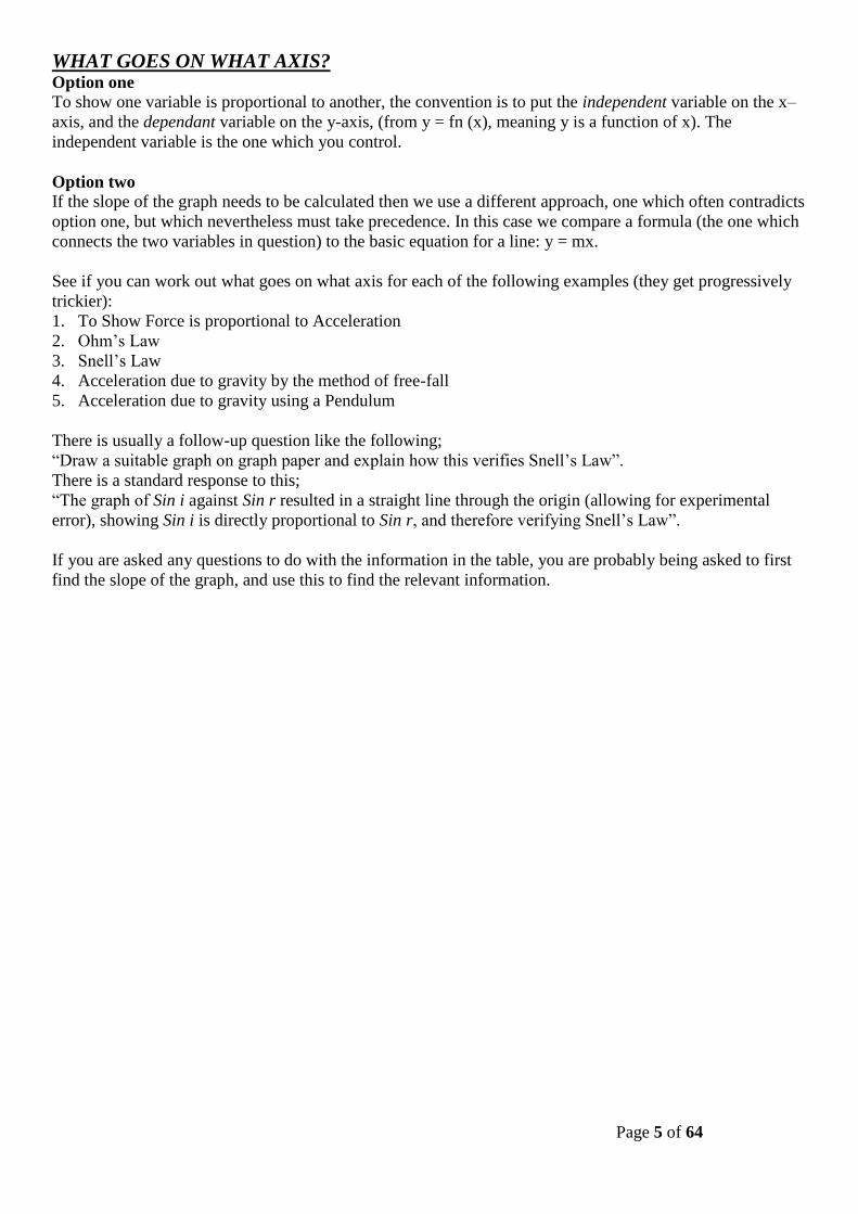
WHAT GOES ON WHAT AXIS?
Option one
To show one variable is proportional to another, the convention is to put the independent variable on the x–
axis, and the dependant variable on the y-axis, (from y = fn (x), meaning y is a function of x). The
independent variable is the one which you control.
Option two
If the slope of the graph needs to be calculated then we use a different approach, one which often contradicts
option one, but which nevertheless must take precedence. In this case we compare a formula (the one which
connects the two variables in question) to the basic equation for a line: y = mx.
See if you can work out what goes on what axis for each of the following examples (they get progressively
trickier):
1. To Show Force is proportional to Acceleration
2. Ohm’s Law
3. Snell’s Law
4. Acceleration due to gravity by the method of free-fall
5. Acceleration due to gravity using a Pendulum
There is usually a follow-up question like the following;
“Draw a suitable graph on graph paper and explain how this verifies Snell’s Law”.
There is a standard response to this;
“The graph of Sin i against Sin r resulted in a straight line through the origin (allowing for experimental
error), showing Sin i is directly proportional to Sin r, and therefore verifying Snell’s Law”.
If you are asked any questions to do with the information in the table, you are probably being asked to first
find the slope of the graph, and use this to find the relevant information.

Page 6 of 64
SUMMARY OF THE GRAPHS

Page 7 of 64
SECTION A: THEORY QUESTIONS
Most of the questions in Section A are repetitive and very straightforward once you have prepared
properly.(i.e. Draw a labelled diagram, how the two sets of values were obtained, sources of
error/precautions, etc. )
Usually these standard questions will then be followed by one or two tricky questions which are looking to
test for a deeper understanding of what’s going on.
I have highlighted the most common of these below.
Why is it important to keep (variable X) constant throughout the experiment?
Answer:
You can only investigate the relationship between two variables at any one time and variable X would be a
third variable.
Why should room temperature be approximately half-way between initial and final temperature (for
Heat experiments)?
Answer:
So that the heat lost to the environment when the system is above room temperature will cancel out the heat
taken in from the environment when the system is below room temperature.
What is the advantage in keeping the length/time/mass as large as possible?
Answer:
A larger length/time/mass would result in a smaller percentage error.
All of the following are taken from past papers.
Make sure when answering these that you check your answer against the appropriate marking
scheme; knowing the answer in your head and writing it down in such a way that you get full marks
in an exam can be two very, very different things.
Here you have most common theory questions from section A:
Measurement of the focal length of a concave mirror (i) How was an approximate value for the focal length found?
(ii) What was the advantage of finding the approximate value for the focal length?
Verification of Snell’s law of refraction / to measure the refractive index of a glass block
(i) Why would smaller values lead to a less accurate result?
Measurement of the focal length of a convex lens (i) Why is it difficult to measure the image distance accurately?
(ii) Give two precautions that should be taken when measuring the image distance.
(iii)What difficulty would arise if the student placed the object 10 cm from the lens?
Measurement of the specific heat capacity of water
(i) Explain why adding a larger mass of copper would improve the accuracy of the experiment.
Page 8 of 64
Measurement of the specific latent heat of fusion of ice
(i) Why was melting ice used?
(ii) Why was dried ice used?
(iii)Explain why warm water was used.
(iv) What should be the approximate room temperature to minimise experimental error?
(v) What was the advantage of having the room temperature approximately halfway between the initial
temperature of the water and the final temperature of the water?
Measurement of the specific latent heat of vaporisation of water
(i) How was the water cooled below room temperature?
(ii) How was the steam dried?
(iii)Why was dry steam used?
(iv) Why was a sensitive thermometer used?
(v) A thermometer with a low heat capacity was used to ensure accuracy. Explain why.
To measure the resistivity of the material of a wire
(i) Why did the student measure the diameter of the wire at different places?
(ii) The experiment was repeated on a warmer day. What effect did this have on the measurements?
(iii)Give two precautions that should be taken when measuring the length of the wire.
To investigate the variation of the resistance of a thermistor with temperature
(i) Use your graph to estimate the average variation of resistance per Kelvin in the range 45 °C – 55 °C.
(ii) In this investigation, why is the thermistor usually immersed in oil rather than in water?
To investigate the variation of current with potential difference for copper electrodes in a copper-
sulphate solution (i) What was observed at the electrodes as current flowed through the electrolyte?
(ii) Draw a sketch of the graph that would be obtained if inactive electrodes were used in this experiment.
To investigate the variation of current with potential difference for a semiconductor diode
(i) What is the function of the 330 Ω resistor in this circuit?
(ii) The student continued the experiment with the connections to the semiconductor diode reversed.
What adjustments should be made to the circuit to obtain valid readings?
(iii) Draw a sketch of the graph obtained for the diode in reverse bias.
To verify joule’s law
(i) Why was a fixed mass of water used throughout the experiment?
(ii) Given that the mass of water in the calorimeter was 90 g in each case, and assuming that all of the
electrical energy supplied was absorbed by the water, use the graph to determine the resistance of the
heating coil.
The specific heat capacity of water is 4200 J kg–1 K–1.
(iii)Explain why the current was allowed to flow for a fixed length of time in each case.
Measurement of acceleration due to gravity (g) using the freefall method
(i) Indicate the distance s on your diagram.
(ii) Describe how the time interval t was measured.
(iii)Give two ways of minimising the effect of air resistance in the experiment.
To show that acceleration is proportional to the force which caused it
(i) How was the effect of friction reduced in the experiment?
(i) Using your graph, find the mass of the body.

Page 9 of 64
(ii) On a trial run of this experiment, a student found that the graph did not go through the origin.
Suggest a reason for this.
(iii)Describe how the apparatus should be adjusted, so that the graph would go through the origin.
To verify the principle of conservation of momentum
(i) How could the accuracy of the experiment be improved?
(ii) How did the student know that body A was moving at constant velocity?
(iii)How were the effects of friction and gravity minimised in the experiment?
Verification of Boyle’s law
(i) Why should there be a delay between adjusting the pressure of the gas and recording its value?
(ii) Describe how the student ensured that the temperature of the gas was kept constant.
Investigation of the laws of equilibrium for a set of co-planar forces
(i) Describe how the centre of gravity of the metre stick was found.
(ii) How did the student know that the metre stick was in equilibrium?
(iii)Why was it important to have the spring balances hanging vertically?
Investigation of the relationship between periodic time and length for a simple pendulum and hence
calculation of g
(i) Give two factors that affect the accuracy of the measurement of the periodic time.
(ii) Why did the student measure the time for 30 oscillations instead of measuring the time for one?
(iii)How did the student ensure that the length of the pendulum remained constant when the pendulum was
swinging?
(iv) Explain why a small heavy bob was used.
(v) Explain why the string was inextensible.
(vi) Describe how the pendulum was set up so that it swung freely about a fixed point.
To measure the speed of sound in air
(i) How was it known that the air column was vibrating at its first harmonic?
Investigation of the variation of fundamental frequency of a stretched string with length (i) How did the student know that the string was vibrating at its fundamental frequency?
Investigation of the variation of fundamental frequency of a stretched string with tension
(i) Why was it necessary to keep the length constant?
(ii) How did the student know that the string was vibrating at its fundamental frequency?
(iii)How did the student know that resonance occurred?
(iv) Use your graph to calculate the mass per unit length of the string.
Measurement of the wavelength of monochromatic light
(i) What effect would each of the following changes have on the bright images formed:
using a monochromatic light source of longer wavelength
using a diffraction grating having 200 lines per mm
using a source of white light instead of monochromatic light?
(ii) Calculate the maximum number of images that are formed on the screen.
(iii)The laser is replaced with a source of white light and a series of spectra are formed on the screen.
Explain how the diffraction grating produces a spectrum.
(iv) Explain why a spectrum is not formed at the central (zero order) image.
(v) The values for the angles on the left of the central image are smaller than the corresponding ones on the
right. Suggest a possible reason for this.

Page 10 of 64
EXPERIMENT QUESTIONS (SECTION A) BY YEAR
Experiment Title 13 12 11 10 09 08 07 06 05 04 03 02
Concave Mirror
3 3
Convex Lens
2 2 3
Refractive Index
3 3
Verify F = Ma
1
g by free-fall
1 1
Conservation of Momentum
1 1
Simple Pendulum
1 1 1
Calibration Curve
Specific Heat Capacity
2
Latent Heat of Vapourisation
2 2 2
Latent Heat of Fusion
2 2
Boyle’s Law
2 2 1
Laws of Equiblibrium
1 1 1
Speed of Sound
3
Natural Frequency and Length
3 3
Natural Frequency and Tension
3 3 3
Wavelength of Light
3 3 2 2
Joule’s Law
4 4
Ohm’s Law
4
V I for a Filament Bulb
4
V I for copper sulphate
4 4
Semiconductor Diode
4 4
R versus Temp for a Metal
4
R versus Temp for Thermistor
4
Resistivity 4
4

Page 11 of 64
MEASUREMENT OF THE FOCAL LENGTH OF A CONCAVE MIRROR
APPARATUS: Concave mirror, screen, lamp-box with crosswire, metre stick, retort stand.
DIAGRAM
Procedure
1. Place the ray-box well outside the approximate focal length.
2. Move the screen until a clear inverted image of the crosswire is obtained.
3. Measure the distance u from the crosswire to the mirror, using the metre stick.
4. Measure the distance v from the screen to the mirror.
5. Repeat this procedure for different values of u.
6. Calculate the focal length of the mirror using the formula vuf
111 and get an average.
7. Plot a graph of 1/u against 1/v and use the intercepts to get two values for f. Then get the average of these two.
RESULTS
CONCLUSION
Using the graph we got an average value for the focal length of the mirror of 25.6 cm.
From the table of data we got an average value of 24.4 cm, which was close to the value we got from the graph,
suggesting that both readings are reasonably accurate.
SOURCES OF ERROR / PRECAUTIONS
1. Determining when the image was in sharpest focus; repeat each time and get an average.
2. Parallax error associated with measuring u and v; ensure your line of sight is at right angles to the metre stick.
3. Take all measurements from the centre of the mirror.
NOTES
How to find an approximate value for the focal length.
1. Focus the image of a distant object onto a screen.
2. Measure the distance between the mirror and the screen.
3. This corresponds to an approximate value for the focal length of the mirror.
Object
distance u
1/u
Image
distance v
1/v
Focal
Length f

Page 12 of 64
EXPLANATION OF THE GRAPH:
FORMULA: vuf
111 FUNCTION: y = mx + C
Calculate 1/u and 1/v values Label axes
Plot all points 1/v Straight line Extrapolate to cut axis (or axes) Read axis (or axes) value =
Focal length =
1/u
The graph of 1/u against 1/v (on the y-axis) is a straight line.
You know from your maths that any straight line cuts the x-axis when y=0
In our case, the line vuf
111 cuts the 1/u axis when 1/v = 0
Giving 1/u + 0 = 1/v the value of 1/u where line cuts 1/u axis is 1/f
Similarly the value of 1/v where line cuts 1/v axis is 1/f
EXAM QUESTIONS: 2007(Q3), 2013(Q3)
SAMPLE:
2007(Q3)
In an experiment to measure the focal length of a concave mirror, an approximate value for the focal length was found. The image distance v was then found for a range of values of the object distance u. The following data was recorded. 1. How was an approximate value for the focal length found? 2. What was the advantage of finding the approximate value for the focal length? 3. Describe, with the aid of a labelled diagram, how the position of the image was found. 4. Calculate the focal length of the concave mirror by drawing a suitable graph based on the recorded data.
u/cm 15.0 20.0 25.0 30.0 35.0 40.0
v/cm 60.5 30.0 23.0 20.5 18.0 16.5
Page 13 of 64
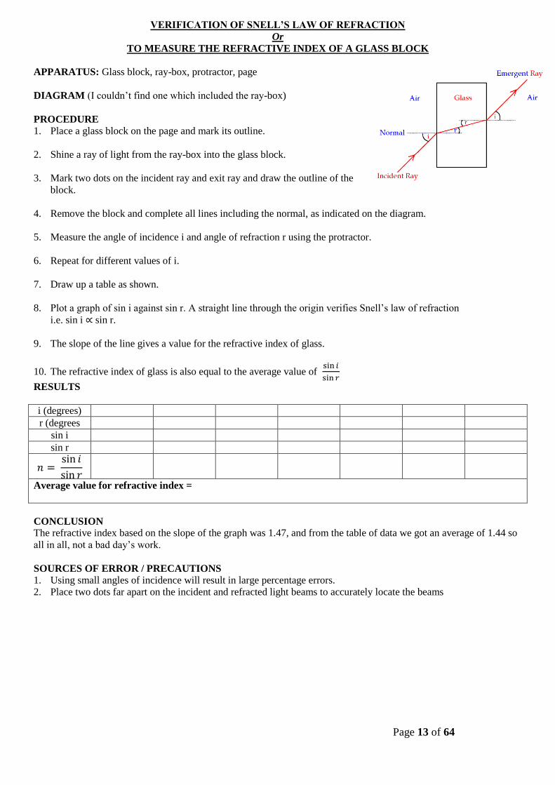
VERIFICATION OF SNELL’S LAW OF REFRACTION
Or
TO MEASURE THE REFRACTIVE INDEX OF A GLASS BLOCK
APPARATUS: Glass block, ray-box, protractor, page
DIAGRAM (I couldn’t find one which included the ray-box)
PROCEDURE 1. Place a glass block on the page and mark its outline.
2. Shine a ray of light from the ray-box into the glass block.
3. Mark two dots on the incident ray and exit ray and draw the outline of the
block.
4. Remove the block and complete all lines including the normal, as indicated on the diagram.
5. Measure the angle of incidence i and angle of refraction r using the protractor.
6. Repeat for different values of i.
7. Draw up a table as shown.
8. Plot a graph of sin i against sin r. A straight line through the origin verifies Snell’s law of refraction
i.e. sin i ∝ sin r.
9. The slope of the line gives a value for the refractive index of glass.
10. The refractive index of glass is also equal to the average value of sin 𝑖
sin 𝑟
RESULTS
i (degrees)
r (degrees
sin i
sin r
𝑛 = sin 𝑖
sin 𝑟
Average value for refractive index =
CONCLUSION
The refractive index based on the slope of the graph was 1.47, and from the table of data we got an average of 1.44 so
all in all, not a bad day’s work.
SOURCES OF ERROR / PRECAUTIONS
1. Using small angles of incidence will result in large percentage errors.
2. Place two dots far apart on the incident and refracted light beams to accurately locate the beams

Page 14 of 64
EXPLANATION OF THE GRAPH:
FORMULA: 𝑛 = sin 𝑖
sin 𝑟 FUNCTION: y = mx
Calculate sin i and sin r values Label axes
Plot all points
A straight line through the origin
verifies Snell’s law of refraction
i.e. sin i ∝ sin r.
The slope of the line gives a value for
the refractive index of glass Refractive index = slope = y2 – y1
/ x2
– x1
EXAM QUESTIONS: 2005(Q3), 2010(Q3)
SAMPLE:
2005(Q3)
In an experiment to verify Snell’s law, a student measured the angle of incidence i and the angle of refraction r for a ray of light entering a substance. This was repeated for different values of the angle of incidence. The following data was recorded. (i) Describe, with the aid of a diagram, how the student obtained the angle of refraction. (ii) Draw a suitable graph on graph paper and explain how your graph verifies Snell’s law. (iii) From your graph, calculate the refractive index of the substance. (iv) The smallest angle of incidence chosen was 200.
Why would smaller values lead to a less accurate result?
i/degrees 20 30 40 50 60 70
r/degrees 14 19 26 30 36 40

Page 15 of 64
TO FIND THE REFRACTIVE INDEX OF A LIQUID BY MEASURING THE REAL DEPTH AND THE
APPARENT DEPTH OF AN OBJECT IN THE LIQUID
APPARATUS: Beakers, mirror, retort stand, cork, pins, metre stick
DIAGRAM
PROCEDURE 1. Fill beaker with water and place pin at the centre of the base of
2. the beaker. This pin is the object.
3. Place the plane mirror accross the top of the beaker.Make sure the
4. water is not touching the back of the mirror
5. Stick the second pin in the cork of the retort stand. Adjust the position of the secomd pin until its image in the
plane mirror is in line with the image of the first pin in the water.
6. Adjust the height of the second pin until there is no parallax between the two images.
7. Measure with the metre stick:
a. -the distance from the object pin to the top of the beaker.
b. -the distance from the second pin to the top of the water.
8. Record these values.
9. complete the table below
RESULTS
Real depth Apparent depth Real depth / Apparent depth
Real depth / Apparent depth is the refractive index of liquid
SOURCES OF ERROR / PRECAUTIONS
Errors arise both in locating the position of no parallax and in measuring the distances with the metre stick
Page 16 of 64
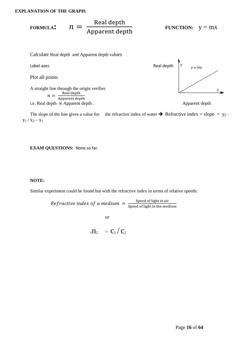
EXPLANATION OF THE GRAPH:
FORMULA: 𝑛 = Real depth
Apparent depth FUNCTION: y = mx
Calculate Real depth and Apparent depth values Label axes Real depth
Plot all points
A straight line through the origin verifies
𝑛 = Real depth
Apparent depth
i.e. Real depth ∝ Apparent depth . Apparent depth
The slope of the line gives a value for the refractive index of water Refractive index = slope = y2 –
y1 / x2
– x1
EXAM QUESTIONS: None so far.
NOTE:
Similar experiment could be found but with the refractive index in terms of relative speeds:
𝑅𝑒𝑓𝑟𝑎𝑐𝑡𝑖𝑣𝑒 𝑖𝑛𝑑𝑒𝑥 𝑜𝑓 𝑎 𝑚𝑒𝑑𝑖𝑢𝑚 = Speed of light in air
Speed of light in the medium
or
1n2 = c1 / c2

Page 17 of 64
MEASUREMENT OF THE FOCAL LENGTH OF A CONVEX LENS
APPARATUS Converging lens, screen, lamp-box with crosswire, metre stick, retort stand.
DIAGRAM
PROCEDURE
1. Place the ray-box well outside the approximate focal length.
2. Move the screen until a clear inverted image of the crosswire is obtained.
3. Measure the distance u from the crosswire to the lens, using the metre stick.
4. Measure the distance v from the screen to the lens.
5. Repeat this procedure for different values of u.
6. Calculate the focal length of the lens each time using the formula vuf
111 and get an average.
7. Plot a graph of 1/u against 1/v and use the intercepts to get two values for f. Then get the average of these two.
RESULTS
Object
distance u
1/u
Image
distance v
1/v
Focal
Length f
CONCLUSION
Using the graph we got an average value for the focal length of the lens of 25.6 cm.
From the table of data we got an average value of 24.4 cm, which was close to the value we got from the graph,
suggesting that both readings are reasonably accurate.
SOURCES OF ERROR / PRECAUTIONS
4. Determining when the image was in sharpest focus; repeat each time and get an average.
5. Parallax error associated with measuring u and v; ensure your line of sight is at right angles to the metre stick.
6. Take all measurements from the centre of the lens.
NOTES
How to find an approximate value for the focal length.
4. Focus the image of a distant object onto a screen.
5. Measure the distance between the lens and the screen.
6. This corresponds to an approximate value for the focal length of the lens.

Page 18 of 64
EXPLANATION OF THE GRAPH:
FORMULA: vuf
111 FUNCTION: y = mx + C
Calculate 1/u and 1/v values Label axes
Plot all points Straight line Extrapolate to cut axis (or axes) Read axis (or axes) value =
Focal length =
Using the graph to calculate the focal length
It is also possible to draw a graph, on graph paper, of 1/v (y-axis) against 1/u.
The equation of the line can be compared to the standard form of linear equation, y = mx + c.
In this case it is: 1/v = -1/u + 1/f. This cuts (intercepts) the y-axis (1/v axis) when x (1/u) is zero
i.e. 1/v = 0 + 1/f. Similarly the line intercepts the 1/u axis when 1/v is zero, giving us 1/u = 1/f.
From your graph get the average of the two intercepts, find the reciprocal to get the value of f.
EXAM QUESTIONS: 2003(Q3), 2009(Q3), 2012(Q3)
SAMPLE:
2012(Q3)
In an experiment to measure the focal length of a converging lens, a student measured the image distance v
for each of four different values of the object distance u.
The table shows the data recorded by the student.
u/cm 12.0 18.0 23.6 30.0
v/cm 64.5 22.1 17.9 15.4
(iv) Describe, with the aid of a labelled diagram, how the student obtained the data.
(v) Why is it difficult to measure the image distance accurately?
(vi) Using all of the data in the table, find the value for the focal length of the lens.
(vii) Why is it difficult to measure the image distance when the object distance is less than 10 cm?

Page 19 of 64
TO CALIBRATE A THERMOMETER USING THE LABORATORY MERCURY THERMOMETER AS A
STANDARD
APPARATUS
Mercury thermometer, unmarked thermometer, heat source, beaker of water, ruler.
DIAGRAM:
PROCEDURE 1. Set up apparatus as shown in the diagram.
2. Record the temperature θ, in °C, from the mercury thermometer and the corresponding length of alcohol in the
blank thermometer.
3. Allow the temperature of the water to increase by about 5 °C.
4. Repeat the procedure until at least ten sets of readings have been recorded.
5. Plot a graph of length l against temperature θ.
6. An unknown temperature can now be determined using the blank thermometer by noting the length of alcohol at
this temperature and then using the graph to calculate the temperature.
RESULTS
Temperature (θ) Length (cm)
CONCLUSION
When we plotted our results we got a reasonably straight line. We then tested our graph using some lukewarm water.
We got a length of 15cm on the blank thermometer and used the graph to give us a temperature of 56 0C. When we
used the mercury thermometer to check our results we got a temperature of 58 0C so all in all it wasn’t a complete
waste of time. Still though, I have to admit I’ve lived through more exciting events.
SOURCES OF ERROR / PRECAUTIONS
1. Heat the water very slowly so that it is easy to take temperature and length readings simultaneously.
2. Have your eye level with the liquid columns when taking temperature and length readings to avoid parallax error.

Page 20 of 64
EXPLANATION OF THE GRAPH:
FORMULA: none Calibration Curve of a thermometer
In this experiment you simply have
to measure (record) the temperature θ, in
°C, from the mercury thermometer and the
corresponding length of alcohol in the
blank thermometer.
The length is the thermometric property. Plot a graph of length l against temperature θ and that way we have the calibration curve of a thermometer.
EXAM QUESTIONS: None at higher level so far. For Ordinary Level: 2007, 2012
SAMPLE:
[2012 OL] You carried out an experiment to establish the calibration curve of a thermometer.
(i) Describe, with the aid of a diagram, the procedure you used in the experiment. (ii) Name the thermometric property of the thermometer you calibrated and describe how the value of this
property was measured. (iii) The following table shows the data obtained in an experiment to establish the calibration curve of a
thermometer.
Using the data in the table, draw a graph on graph paper to establish the calibration curve. Put temperature on the horizontal axis.
(iv) Use your calibration curve to determine the temperature when the value of the thermometric property is 60.
Temperature/ 0C 0 20 40 60 80 100
Value of thermometric property
5 14 29 48 80 130

Page 21 of 64
MEASUREMENT OF THE SPECIFIC HEAT CAPACITY OF WATER
APPARATUS
Power supply, joulemeter, heating coil, calorimeter, thermometer, electronic balance.
DIAGRAM
PROCEDURE
1. Find the mass of the water by first measuring the mass of the empty calorimeter, then the mass of the calorimeter
with water in it, and subtracting one form the other.
2. Set up the apparatus as shown in the diagram (with a power supply connected to the joulemeter).
3. Record the initial temperature of the water (we assume this to be the same temperature as the calorimeter).
4. Switch on the power supply and allow the temperature of the water to rise by about 10 degrees.
5. Switch off the power supply.
6. Note the reading on the joulemeter and the final temperature of the water (and calorimeter).
7. Calculate the specific heat capacity of water (cwater) using the equation:
Energy supplied = (mcΔθ)cal + (mcΔθ)water where Δθ is the change in temperature and ccal is known.
RESULTS
Mass of calorimeter:
Mass of calorimeter + water:
Mass of water:
Initial temperature of water (and calorimeter):
Final temperature of water (and calorimeter):
Change in temperature Δθ:
Joulemeter reading:
CONCLUSION
The theoretical value for the specific heat capacity of water = 4200 J kg–1 K–1. We got an answer of 7.
Conclusion? I need to start copying my answers from someone else.
SOURCES OF ERROR
1. Heat may be gained from or lost to the surroundings.
2. If a mercury thermometer is used, this may only be accurate to the nearest degree.
PRECAUTIONS 1. Ensure that the heating element is covered with water to avoid any loss of heat energy.
2. Ensure that the calorimeter is well insulated to avoid loss of heat energy.
3. Stir the water throughout the experiment to ensure that the thermometer reading reflects the heat supplied.
4. Use a sensitive thermometer graduated to 0.1 or 0.2 degrees. An error of 1 deg. in 10 is a large percentage error.
5. Ensure that room temperature is midway between the initial and final temperatures of the water.

Page 22 of 64
GRAPH: There is no graph for this experiment
FORMULA AND CALCULATIONS:
On the assumption that no heat is given or taken from the surroundings we have:
Energy supplied = (mcΔθ)cal + (mcΔθ)water
where Δθ is the change in temperature and ccal is known.
EXAM QUESTIONS: 2007(Q2)
SAMPLE:
2007(Q2) The specific heat capacity of water was found by adding hot copper to water in a copper calorimeter. This was not the method most students would have used to carry out the experiment so there was much annoyance when it appeared on the paper. Nevertheless it does differentiate between those students who understand the underlying principles and those who have just learned off a formula. The following data was recorded: (ii) Describe how the copper was heated and how its temperature
was measured. (iii) Using the data, calculate the energy lost by the hot copper (iv) Using the data, calculate the specific heat capacity of water. (v) Give two precautions that were taken to minimise heat loss to the surroundings. (vi) Explain why adding a larger mass of copper would improve the accuracy of the experiment.
mass of calorimeter 55.7 g
mass of calorimeter + water 101.2 g
mass of copper + calorimeter + water 131.4 g
initial temperature of water 16.5 oC
temperature of hot copper 99.5 oC
final temperature of water 21.0 oC

Page 23 of 64
MEASUREMENT OF THE SPECIFIC LATENT HEAT OF FUSION OF ICE
APPARATUS: Ice, water, calorimeter, lagging, beakers, kitchen paper, thermometer and electronic balance.
DIAGRAM:
PROCEDURE
1. Place some ice cubes in a beaker of water and keep taking the temperature with the thermometer until the ice-
water mixture reaches 0 °C.
2. Find the mass of the calorimeter.
3. Half fill the calorimeter with water warmed to approximately 10 °C above room temperature.
4. Find the combined mass of the calorimeter and water ice. The mass of the water can be calculated by subtraction.
5. Find the mass of the beaker and its contents. The mass of the ice can be calculated by subtraction.
6. Record the initial temperature (θinitial) of the calorimeter plus water.
7. Crush some ice and dry it carefully with blotting paper or filter paper.
8. Add the pieces of dry crushed ice to the calorimeter. Do this until the temperature of the water has fallen by about
20 °C.
9. Take a note of the lowest temperature reached (θfinal)
10. Use the formula below to calculate a value for the latent heat of fusion of ice.
RESULTS
Mass of calorimeter:
Mass of calorimeter plus water:
Room temperature:
Temperature of ice:
Initial temperature of water (θinitial):
Final temperature of water (θfinal):
Mass of calorimeter plus water plus ice:
CALCULATIONS
The rise in temperature of the ice (θΔmelted ice) = θfinal – 0 °C . . . . . . . . . . .
The fall in temperature of the calorimeter (Δθcal) = is θinitial – θfinal . . . . . . . . . . . .
The fall in temperature of the water (Δθwater) = is θinitial – θfinal . . . . . . . . . . . .
Mass of water:
Mass of ice:
We now have
Heat lost by calorimeter + heat lost by water = Heat gained by ice turning to water + heat gained by melted ice
(mcΔθ)cal + (mcΔθ)water = (ml)ice + (mcΔθ)melted ice
CONCLUSION
The theoretical value for specific latent heat of fusion of ice is 3.3 × 10⁵ J kg-1. We got a value of 7, so obviously
either the theory is crap or I need a new lab partner.

Page 24 of 64
PRECAUTIONS
1. Ensure that the ice is dried (dab it with tissue paper) before adding to the calorimeter.
2. Use warmed water (about 10 deg. above room temp.) at the start of the experiment so that, on average, heat is
neither lost or gained from the surroundings. This also helps the ice to melt more quickly speeding up the expt.
3. Use a well insulated calorimeter to avoid loss or gain of heat to the surroundings.
4. Stir well and record the lowest temperature when all of the ice has melted.
GRAPH: There is no graph for this experiment
EXAM QUESTIONS: 2002(Q2), 2008(Q2)
SAMPLE QUESTIONS:
2008(Q2) In an experiment to measure the specific latent heat of fusion of ice, warm water was placed in a copper calorimeter. Dried, melting ice was added to the warm water and the following data was recorded. Mass of calorimeter 60.5 g Mass of calorimeter + water 118.8 g Temperature of warm water 30.5 oC Mass of ice 15.1 g Temperature of water after adding ice 10.2 oC (vi) Explain why warm water was used. (vii) Why was dried ice used? (viii) Why was melting ice used? (ix) Describe how the mass of the ice was found. (x) What should be the approximate room temperature to minimise experimental error? (xi) Calculate the energy lost by the calorimeter and the warm water. (xii) Calculate the specific latent heat of fusion of ice.
2002(Q2)
In an experiment to measure the specific latent heat of fusion of ice, warm water was placed in an aluminium calorimeter. Crushed dried ice was added to the water. The following results were obtained. Mass of calorimeter.......................................= 77.2 g Mass of water.................................................= 92.5 g Initial temperature of water...........................= 29.4 0C Temperature of ice ........................................= 0 0C Mass of ice.....................................................= 19.2 g Final temperature of water.............................= 13.2 0C Room temperature was 21 0C. (i) What was the advantage of having the room temperature approximately halfway between the initial
temperature of the water and the final temperature of the water? (ii) Describe how the mass of the ice was found. (iii) Calculate a value for the specific latent heat of fusion of ice (iv) The accepted value for the specific latent heat of fusion of ice is 3.3 × 10⁵ J kg-1; suggest two reasons why your
answer is not this value.

Page 25 of 64
MEASUREMENT OF THE SPECIFIC LATENT HEAT OF VAPORISATION OF WATER
APPARATUS
Calorimeter, beaker, conical flask, steam trap, retort
stand, heat source, thermometer, electronic balance.
DIAGRAM
PROCEDURE
1. Find the mass of the calorimeter.
2. Half fill the calorimeter with water cooled to
approximately 10 °C below room temperature.
3. Find the mass of the water plus calorimeter and by
subtraction find the mass of the water.
4. Record the temperature of the calorimeter plus water θinitial
5. Boil the water in the flask until steam issues freely from the delivery tube.
6. Allow dry steam to pass into the water in the calorimeter until the temperature has risen by about 20 °C, then
remove the steam delivery tube from the water.
7. Record the final temperature θfinal of the calorimeter plus water plus condensed steam.
8. Find the mass of the calorimeter plus water plus condensed steam and by subtraction find the mass of the
condensed steam.
RESULTS
Mass of the calorimeter........................... =
Mass of calorimeter plus cold water .................................. =
Initial temperature of water..................... =
Temperature of the steam........................ =
Final temperature of water ...................... =
Final mass of steam calorimeter plus water plus steam ............................... =
CALCULATIONS
Mass of cold water .................................. =
Mass of steam .................................. =
Δθcondensed_steam = . . . . . . . .
Δθcal = . . . . . . . . . . . . .
Δθwater = . . . . . . . . . .
Energy lost by steam + energy lost by condensed steam cooling down = energy gained by calorimeter + energy gained
by the water
mlsteam + mcΔθcondensed_steam = mcΔθcal + mcΔθwater
CONCLUSION:
The theoretical value for the latent heat of vapourisation of water is 2.26 x 10⁶ J kg-1; we got an answer of 7. Therefore
we conclude that this experiment sucks.
PRECAUTIONS:
1. Ensure that only steam (not water) enters the water in the calorimeter. Use a "steam trap" (it actually traps water)
if available
2. Use a tilted insulated tube as an alternative delivery pipe for dry steam. This does away with the need to use a
steam trap.
3. If the water in the calorimeter is initially cooled to10 °C below room temperature and then heated to 10 °C above
room temperature the heat gains and heat losses approximately cancel each other out.
4. Use a well insulated calorimeter to avoid loss or gain of heat to the surroundings
5. Stir well and record the highest temperature when the steam has stopped bubbling into the water.

Page 26 of 64
GRAPH: There is no graph for this experiment
EXAM QUESTIONS: 2003(Q2), 2005(Q2), 2010(Q2)
SAMPLE:
2010(Q2) In an experiment to measure the specific latent heat of vaporisation of water, a student used a copper calorimeter containing water and a sensitive thermometer. The water was cooled below room temperature before adding dry steam to it. The following measurements were recorded.
Mass of copper calorimeter = 34.6 g Initial mass of calorimeter and water = 96.4 g Mass of dry steam added = 1.2 g Initial temperature of calorimeter and cooled water = 8.2 °C Final temperature of calorimeter and water = 20.0 °C
(vi) How was the water cooled below room temperature? (vii) How was the steam dried? (viii) Describe how the mass of the steam was determined. (ix) Why was a sensitive thermometer used? (x) Using the data, calculate the specific latent heat of vaporisation of water.
2005(Q2) In an experiment to measure the specific latent heat of vaporisation of water, cool water was placed in an insulated copper calorimeter. Dry steam was added to the calorimeter. The following data was recorded. Mass of calorimeter = 50.5 g Mass of calorimeter + water = 91.2 g Initial temperature of water = 10 oC Temperature of steam = 100 oC Mass of calorimeter + water + steam = 92.3 g Final temperature of water = 25 oC (i) Calculate a value for the specific latent heat of vaporisation of water. (ii) Why was dry steam used? (iii) How was the steam dried? (iv) A thermometer with a low heat capacity was used to ensure accuracy. Explain why.

Page 27 of 64
TO VERIFY JOULE’S LAW
APPARATUS:
Calorimeter with a lid, heating coil, power supply, rheostat, ammeter, thermometer, stopwatch, electronic balance.
DIAGRAM:
PROCEDURE:
1. Set up the circuit as shown.
2. Note the temperature.
3. Switch on the power and simultaneously start the stopwatch.
4. Make sure the current stays constant throughout; adjust the rheostat if necessary.
5. Note the current using the ammeter and note the time for which the current flowed using the stopwatch.
6. Stir and note the highest temperature. Calculate the change in temperature (θΔ)
7. Repeat the above procedure for increasing values of current I, taking at least six readings.
8. Plot a graph of I2 (y-axis) against θΔ
(x-axis).
RESULTS:
θinitial (0C)
θfinal (0C)
Δθ (0C)
I (A) 0.5 1.0 1.5 2.0 2.5 3.0
I2(A2)
CONCLUSION:
A graph of our results produced a straight-line through the origin thus verifying that Δθ α I2
and therefore verifies
Joule’s law.
PRECAUTIONS:
1. Put sufficient water in the calorimeter to cover the heating coil.
2. Take care not to exceed the current-rating marked on the rheostat and/or the calorimeter.
NOTES
1. See the note in the text-book to see how this experiment (where Δθ α I2) verifies Joule’s Law (P α I2).
2. Allow the coil to heat the water for about five minutes. This must be the same for each run.

Page 28 of 64
FORMULA: Δθ α I2 (Joule’s Law) FUNCTION: y=mx Electrical energy in = Heat energy out RI2 t = mcΔθ
GRAPH:
Label axes A straight line through origin shows that ∆ϑ ∝ I2 which verifies Joule’s Law.
The slope of the line can lead you to
find the value of the Resistance ( R )
of the heating coil if the
mass (m) of water to be heated is
constant and the time (t) that the
current flows through the heating
coil is constant too:
∆ϑ is in the y-axis and I2 in the x-axis
Since:
Electrical energy in = Heat energy out RI2 t = mcΔθ Therefore: Δθ = (R t/mc) I2
So the slope =(R t/mc)
EXAM QUESTIONS: 2006(Q4), 2003(Q4)
SAMPLE:
[2003 HL] In an experiment to verify Joule’s law, a heating coil was placed in a fixed mass of water. The temperature rise Δθ produced for different values of the current I passed through the coil was recorded.
In each case the current was allowed to flow for a fixed length of time. The table shows the recorded data. (i) Describe, with the aid of a labelled diagram, how the apparatus was arranged in this experiment. (ii) Using the given data, draw a suitable graph on graph paper and explain how your graph verifies Joule’s law. (iii) Explain why the current was allowed to flow for a fixed length of time in each case. (iv) Apart from using insulation, give one other way of reducing heat losses in the experiment.
I /A 1.5 2.0 2.5 3.0 3.5 4.0 4.5
Δθ / °C 3.5 7.0 10.8 15.0 21.2 27.5 33.0

Page 29 of 64
TO MEASURE THE RESISTIVITY OF THE MATERIAL OF A WIRE
APPARATUS:
Length of nichrome wire, micrometer or digital calilpers, ohmmeter, metre stick.
DIAGRAM:
PROCEDURE:
1. Tie a length of nichrome between the bars of the two stands as shown above. Stretch the wire enough to remove
any kinks or ‘slack’ in the wire.
2. Note the resistance of the leads when the crocodile clips are connected together.
3. Connect the crocodile clips to the wire. Read the resistance from the ohmmeter. Subtract the resistance of the
leads to get the resistance R of the wire.
4. Measure the length (L) of the wire between the crocodile clips with the metre stick.
5. Find the diameter (d) of the wire at different points, taking the zero error into account. Find the average value of
the diameter d. We use a digital callipers instead of the micrometer.
6. Calculate the resistivity using the formula ρ =𝑅𝜋𝑑2
4𝐿
7. Repeat using different lengths of wire and calculate an average value for ρ.
RESULTS:
Run
no.
Diameter d
(m)
RTotal
()
RLeads
()
Rnet
()
L
(m) ρ =
𝑅𝜋𝑑2
4𝐿
( m)
1.
2.
3.
Average value for resistivity = ________________ m.
CONCLUSION:
We found an average value for the resistivity of the wire as __________ m.
This is reasonably accurate because all our answers are close together and are reasonably close to the accepted value
of 100 × 10-8
Ω m (at 20 °C).
SOURCES OF ERROR / PRECAUTIONS:
1. Ensure that the wire is straight when measuring its length.
2. Measure only between the inside of the ohmmeter contacts. 3. Make sure to zero the reading on the callipers before starting.
NOTE:
When setting up lay the wire over a metre stick and clamp it to using G-clamps. The length of wire can now be
measured directly.

Page 30 of 64
GRAPH: There is no graph for this experiment
EXAM QUESTIONS: 2004(Q4), 2009(Q4)
SAMPLE:
[2009 HL] In an experiment to measure the resistivity of nichrome, the resistance, the diameter and appropriate length of a sample of nichrome wire were measured. The following data were recorded: Resistance of wire = 7.9 Ω Length of wire = 54.6 cm Average diameter of wire = 0.31 mm (i) Describe the procedure used in measuring the length of the sample of wire. (ii) Describe the steps involved in finding the average diameter of the wire. (iii) Use the data to calculate the resistivity of nichrome. (iv) The experiment was repeated on a warmer day. What effect did this have on the measurements?
[2004 HL]
The following is part of a student’s report of an experiment to measure the resistivity of nichrome wire. “The resistance and length of the nichrome wire were found. The diameter of the wire was then measured at several points along its length.” The following data was recorded. Resistance of wire = 32.1 Ω Length of wire = 90.1 cm Diameter of wire = 0.19 mm, 0.21 mm, 0.20 mm, 0.21 mm, 0.20 mm (i) Name an instrument to measure the diameter of the wire and describe how it is used. (ii) Why was the diameter of the wire measured at several points along its length? (iii) Using the data, calculate a value for the resistivity of nichrome. (iv) Give two precautions that should be taken when measuring the length of the wire.

Page 31 of 64
TO INVESTIGATE THE VARIATION OF THE RESISTANCE OF A METALLIC CONDUCTOR WITH
TEMPERATURE
APPARATUS:
Coil of wire, glycerol, beaker, heat source, thermometer, ohmmeter, boiling tube
DIAGRAM:
PROCEDURE:
1. Set up the apparatus as shown in the diagram.
2. Use the thermometer to note the temperature of the glycerol, which we assume to be the same as the temperature
of the coil.
3. Record the resistance of the coil of wire using the ohmmeter.
4. Heat the beaker and for each 10 °C rise in temperature record the resistance and temperature using the ohmmeter
and the thermometer.
5. Plot a graph of resistance against temperature.
RESULTS:
R ()
θ (0C)
CONCLUSION:
1. From the graph we can see that there is a linear relationship between the temperature of the wire and its resistance,
and that as one increases so does the other.
2. We believe our data to be reliable because it resulted in a straight line which the theory predicted.
PRECAUTIONS / SOURCES OF ERROR:
1. Check for the resistance of the connecting leads and contacts on the ohmmeter. Subtract from later readings
2. Heat very slowly to try to maintain thermal equilibrium between the water and glycerol and coil. When the bunsen
is removed wait until the temperature is steady before taking the resistance readings.
3. Use glycerol in the test tube as it is a better heat conductor than water.

Page 32 of 64
FORMULA: None FUNCTION: y = mx + C (linear function)
GRAPH:
Calculate R and T values Label axes
Plot all points Straight line
EXAM QUESTIONS: 2008(Q4)
SAMPLE:
2008(Q4) A student investigated the variation of the resistance R of a metallic conductor with its temperature θ. The student recorded the following data. (i) Describe, with the aid of a labelled diagram, how the data was obtained. (ii) Draw a suitable graph to show the relationship between the resistance of the metal conductor and its
temperature. (iii) Use your graph to estimate the resistance of the metal conductor at a temperature of –20 oC. (iv) Use your graph to estimate the change in resistance for a temperature increase of 80 oC. (v) Use your graph to explain why the relationship between the resistance of a metallic conductor and its
temperature is linear.
θ/o
C 20 30 40 50 60 70 80
R/Ω 4.6 4.9 5.1 5.4 5.6 5.9 6.1

Page 33 of 64
TO INVESTIGATE THE VARIATION OF THE RESISTANCE OF A THERMISTOR WITH
TEMPERATURE
APPARATUS:
Thermistor, glycerol, beaker, heat source, thermometer, ohmmeter, boiling tube
DIAGRAM:
PROCEDURE:
1. Set up the apparatus as shown in the diagram.
2. Use the thermometer to note the temperature of the glycerol, which we assume to be the same as the temperature of
the thermistor.
3. Record the resistance of the thermistor using the ohmmeter.
4. Heat the beaker and for each 10 °C rise in temperature record the resistance and temperature using the ohmmeter
and the thermometer.
5. Plot a graph of resistance against temperature.
RESULTS:
R ()
θ (0C)
CONCLUSION:
1. From the graph we can see that as temperature increases the resistance decreases.
2. We believe our data to be reliable because it resulted in a smooth curve, which the theory predicted.
PRECAUTIONS / SOURCES OF ERROR:
1. Check for the resistance of the connecting leads and contacts on the ohmmeter. Subtract from later readings.
2. Heat very slowly to try to maintain thermal equilibrium between the water and glycerol and thermistor. When the
bunsen is removed wait until the temperature is steady before taking the resistance readings.
3. Use glycerol in the test tube as it is a better heat conductor than water.
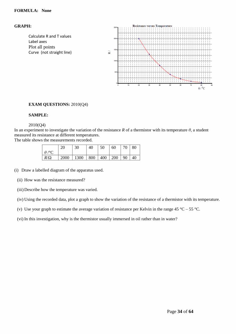
Page 34 of 64
FORMULA: None
GRAPH:
Calculate R and T values Label axes
Plot all points Curve (not straight line)
EXAM QUESTIONS: 2010(Q4)
SAMPLE:
2010(Q4) In an experiment to investigate the variation of the resistance R of a thermistor with its temperature θ, a student
measured its resistance at different temperatures.
The table shows the measurements recorded.
(i) Draw a labelled diagram of the apparatus used.
(ii) How was the resistance measured?
(iii) Describe how the temperature was varied.
(iv) Using the recorded data, plot a graph to show the variation of the resistance of a thermistor with its temperature.
(v) Use your graph to estimate the average variation of resistance per Kelvin in the range 45 °C – 55 °C.
(vi) In this investigation, why is the thermistor usually immersed in oil rather than in water?
θ /°C
20 30 40 50 60 70 80
R/Ω 2000 1300 800 400 200 90 40

Page 35 of 64
TO INVESTIGATE THE VARIATION OF CURRENT (I) WITH P.D. (V) FOR COPPER ELECTRODES IN
A COPPER-SULPHATE SOLUTION
APPARATUS:
Low voltage power supply, rheostat, voltmeter, ammeter, copper electrodes in a copper-sulphate solution.
DIAGRAM:
PROCEDURE:
1. Set up the circuit as shown.
2. Record the potential difference (V) and the current (I) using the voltmeter and ammeter respectively.
3. Adjust the rheostat to obtain different values for V and I.
4. Obtain at least six values for V and I.
5. Plot a graph of I against V.
RESULTS:
V (V)
I (A)
CONCLUSION:
1. We obtained a straight line through the origin therefore the current through the copper-sulphate solution is
proportional to the potential difference across it.
2. We believe our results to be reliable because they resulted in a straight line through the origin, as the theory
predicted.
SOURCES OF ERROR:
1. The copper-sulphate solution may not be concentrated enough.
2. The copper electrodes may have become oxidised and will no longer conduct.
PRECAUTIONS:
1. Sand the electrodes beforehand.
Page 36 of 64
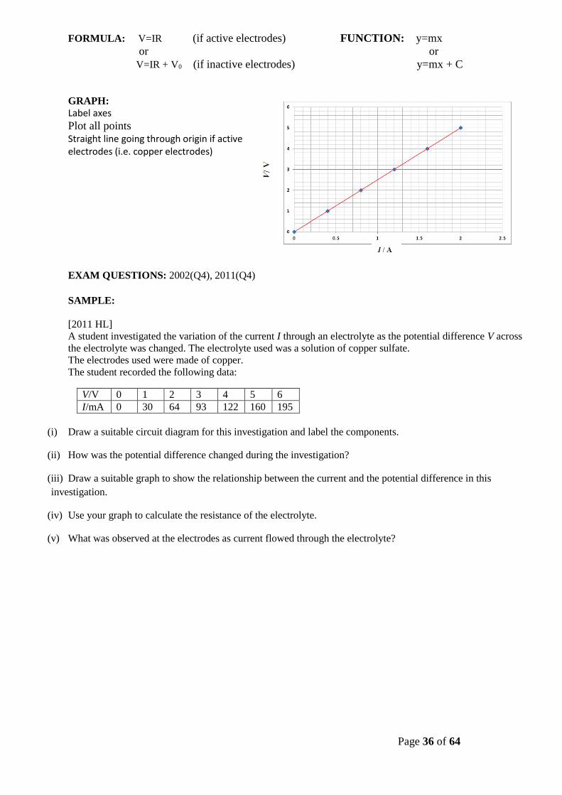
FORMULA: V=IR (if active electrodes) FUNCTION: y=mx
or or
V=IR + V0 (if inactive electrodes) y=mx + C
GRAPH:
Label axes
Plot all points Straight line going through origin if active electrodes (i.e. copper electrodes)
EXAM QUESTIONS: 2002(Q4), 2011(Q4)
SAMPLE:
[2011 HL]
A student investigated the variation of the current I through an electrolyte as the potential difference V across
the electrolyte was changed. The electrolyte used was a solution of copper sulfate.
The electrodes used were made of copper.
The student recorded the following data:
(i) Draw a suitable circuit diagram for this investigation and label the components.
(ii) How was the potential difference changed during the investigation?
(iii) Draw a suitable graph to show the relationship between the current and the potential difference in this
investigation.
(iv) Use your graph to calculate the resistance of the electrolyte.
(v) What was observed at the electrodes as current flowed through the electrolyte?
V/V 0 1 2 3 4 5 6
I/mA 0 30 64 93 122 160 195

Page 37 of 64
TO INVESTIGATE THE VARIATION OF CURRENT (I) WITH P.D. (V) FOR A METALLIC
CONDUCTOR AND HENCE CALCULATE THE RESISTANCE (OHM’S LAW)
APPARATUS:
Low voltage power supply, rheostat, voltmeter, ammeter, length of nichrome wire.
DIAGRAM:
PROCEDURE:
6. Set up the circuit as shown.
7. Record the potential difference (V) and the
current (I) using the voltmeter and ammeter
respectively.
8. Adjust the potential divider to obtain different
values for V and I.
9. Obtain at least six values for V and I.
10. Plot a graph of I against V.
11. Calculate the slope of the graph.
If plotting V on the y-axis and I on the x-axis then the slope of t he graph corresponds to the resistance of the
metallic conductor.
If plotting V on the x-axis and I on the y-axis then the slope of t he graph corresponds to the inverse of the
resistance of the metallic conductor.
RESULTS:
V (V)
I (A)
CONCLUSION:
3. Our graph resulted in a straight line through the origin which implies that the current is directly proportional to the
potential difference.
4. We believe our results to be reliable because they resulted in a straight line through the origin, as the theory
predicted.
5. The resistance of the wire may be determined from the reciprocal of the slope of the graph.
PRECAUTIONS: 1. Use a low voltage so that the current flowing will be small enough that the temperature of the wire stays constant.
2. Use a sensitive milli-ammeter and voltmeter to get accurate readings.
NOTES:
A varying voltage can be obtained from a fixed supply voltage by using a potential divider. It consists of a variable
resistor or fixed resistors in series. Move the slider to change the output voltage. This results in the output voltage
from the potential divider being a fraction of the input voltage.
Normally we would put V on the y-axis and I on the x-axis, and therefore the slope of the graph would correspond to
the resistance. In this case however calculating the resistance is not the main focus of the experiment; the main focus
is to investigate how the current depends upon the potential difference. That is why we put the independent variable
(the one we have control over) on the x-axis. Hence current goes on the y-axis.
We use the same approach for all of the variations (filament bulb, copper sulphate, semi-conductor diode).
For the coil of wire you could use a separate rheostat. The two connections in this are both at the bottom.
Alternatively you could use 1 m of 26 s.w.g. nichrome wire wound on a plastic comb. This has a resistance of
approximately 7.0 Ω.

Page 38 of 64
FORMULA: V=IR (Ohm’s Law) FUNCTION: y=mx
GRAPH:
Label axes
Plot all points A straight line through the origin
verifies Ohm’s law of refraction
i.e. V ∝ I.
The slope of the line gives a value for the
resistance if V is in the y-axis and I in the x-
axis
Resistance = slope = y2 – y1
/ x2
– x1
VERY IMPORTANT NOTE:
Sometimes you may get a graph that is not fully linear, that it’s a bit curvy at the end almost not following
Ohm’s law V=IR where R is the resistance (slope of the graph). R should be a constant value if the temperature of the
metallic conductor does not change. But inevitably, sometimes the temperature of the metallic conductor will increase,
and then we know that the resistance of the metallic conductor will increase too . That increase in resistance in the
metallic conductor will cause an increase of voltage across the metallic conductor (i.e. in that area of the graph the
voltage will not be directly proportional to the current, it will be a bit bigger than expected from Ohm’s Law)
EXAM QUESTIONS: 2013(Q4),
SAMPLE:
2013 Question 4
A student was asked to investigate the variation of current with potential difference for a thin
metallic conductor.
The student set up a circuit using appropriate equipment.
The student recorded the values of the current I passing through the conductor for the corresponding
values of potential difference V.
The recorded data are shown in the table.
(i) Draw and label the circuit diagram used by the student.
(ii) Name the device in the circuit that is used to vary the potential difference across the conductor.
(iii) Explain how the student used this device to vary the potential difference.
(iv) Use the data in the table to draw a graph on graph paper to show the variation of current with
potential difference.
(v) Use your graph to find the value of the resistance of the conductor when the current is 0.7 A.
(vi) Explain the shape of your graph.
V/V 1.0 2.0 3.0 4.0 5.0 6.0
I/A 0.17 0.34 0.50 0.64 0.77 0.88

Page 39 of 64
TO INVESTIGATE THE VARIATION OF CURRENT (I) WITH P.D. (V) FOR A FILAMENT BULB
APPARATUS:
Low voltage power supply, rheostat, voltmeter, ammeter, filament bulb.
DIAGRAM:
PROCEDURE:
1. Set up the circuit as shown (replace the letter X with A for ammeter above, and don’t write this into your report).
2. Record the potential difference (V) and the current (I) using the voltmeter and ammeter respectively.
3. Adjust the potential divider to obtain different values for V and I.
4. Obtain at least six values for V and I.
5. Plot a graph of I against V.
RESULTS:
V (V)
I (A)
CONCLUSION:
1. As the potential difference across the bulb increases so does the current, but not in a linear fashion therefore the
two are not directly proportional.
2. We believe our results to be reliable because they resulted in a smooth curve, as the theory predicted.
QUESTION:
1. Why does the graph start to level off at the end?
2. Why does this happen for the filament bulb but not for the coil of wire (metallic conductor) in the last experiment?
NOTES:
A varying voltage can be obtained from a fixed supply voltage by using a potential divider. It consists of a variable
resistor or fixed resistors in series. Move the slider to change the output voltage. This results in the output voltage
from the potential divider being a fraction of the input voltage.

Page 40 of 64
FORMULA: None
GRAPH:
Label axes Current v Voltage Plot all points
The relationship between current and potential difference for a filament lamp is non linear / not proportional
EXAM QUESTIONS: 2005(Q4),
SAMPLE:
2005(Q4)
A student investigated the variation of the current I flowing through a filament bulb for a range of different values of potential difference V.
(i) Draw a suitable circuit diagram used by the student. (ii) Describe how the student varied the potential difference. (iii) The student drew a graph, as shown, using data recorded in
the experiment. With reference to the graph, explain why the current is not proportional to the potential difference.
(iv) With reference to the graph, calculate the change in resistance of the filament bulb as the potential difference increases from 1 V to 5 V.
(v) Give a reason why the resistance of the filament bulb changes.
.

Page 41 of 64
INVESTIGATE THE VARIATION OF CURRENT (I) WITH P.D. (V) FOR A SEMICONDUCTOR DIODE
IN FORWARD BIAS
APPARATUS: Low voltage power supply, rheostat, voltmeter, ammeter, 330 Ω resistor, semiconductor diode DIAGRAM:
PROCEDURE: 1. Set up the circuit with the semiconductor diode in forward bias as shown. 2. Adjust the potential divider to obtain different values for the voltage V and hence for the current I. 3. Obtain at least ten values for V and for I using the voltmeter and the ammeter. 4. Plot a graph of I against V and join the points in a smooth, continuous curve. RESULTS:
V (volts)
I (milli-amps)
CONCLUSION: We can see from the graph that almost no current flows until the applied voltage exceeds 0.6 V for a silicon diode but then the current rises rapidly. GRAPH: Label axes Current v Voltage
Plot all points
The relationship between current and potential difference for a semiconductor diode is non linear / not proportional
FORMULA: None NOTE: A protective resistor, e.g. 330 Ω, should always be used in series with a diode in forward bias. Therefore even if the diode offers no resistance there will still be some other resistance in the circuit preventing the current getting too high. A germanium diode, e.g. OA91, gives very little current between 0 and 0.2 V but the current then increases rapidly above this voltage. A light emitting diode gives very little current up to 1.6 V but then the current rises rapidly accompanied by the emission of light.

Page 42 of 64
TO INVESTIGATE THE VARIATION OF CURRENT (I) WITH P.D. (V) FOR A SEMICONDUCTOR
DIODE IN REVERSE BIAS
APPARATUS:
Low voltage power supply, rheostat, voltmeter, ammeter, semiconductor diode.
DIAGRAM:
PROCEDURE:
1. Set up the circuit as above and set the
voltage supply at 20 V.
2. The micro-ammeter is used in this part of the experiment, as current values will be very low when a diode is in
reverse bias.
3. Adjust the potential divider to obtain different values for the voltage V and hence for the current I.
4. Obtain at least six values for V (0-20 V) and for I using the voltmeter and the micro-ammeter. Higher voltage
values are required for conduction in reverse bias.
5. Plot a graph of I against V and join the points in a smooth, continuous curve.
RESULTS:
V
(volts)
I
(micro-
amps)
CONCLUSION:
We found no current in reverse bias. In theory there should be a very small amount of current but it was too small to
be detected with our equipment.
PRECAUTIONS / SOURCES OF ERROR:
1. Use a microammeter when the diode is reverse biased as the current flowing is extremely small.
2. Change the positions of the microammeter and voltmeter (reverse biased) so that the current flowing through the
diode is the only one registered in the microammeter (not current through the voltmeter)
NOTES:
The position of the voltmeter has changed since a reverse biased diode has a very large resistance that is greater than
the resistance of most voltmeters. It is essential that the micro-ammeter reads only the current flowing through the
reverse biased diode as the sum of the currents flowing through the voltmeter and reverse biased diode may be much
larger.
Since the resistance of the micro-ammeter is negligible compared with the resistance of the reverse biased diode the
potential difference across the micro-ammeter and diode is almost the same as the potential difference across the diode
alone.
When using a silicon diode it is very difficult to detect the current in reverse bias as the current is so small and
changes very little with temperature variations.
For a germanium diode some reverse current can be detected (a few μA) at 4 V reverse bias. This conduction increases
rapidly when the diode is heated (by hand).

Page 43 of 64
MEASUREMENT OF VELOCITY USING A TICKER-TAPE TIMER
APPARATUS: Ticker timer and tape, low-voltage a.c. power supply, trolley, runway.
DIAGRAM
PROCEDURE
1. Set up the apparatus as in the diagram.
2. Connect the ticker timer to a low-voltage power supply.
3. Give the trolley a small push to start it moving.
4. Adjust the angle of inclination of the runway until the trolley moves with constant velocity, i.e. the spots on the
tape are all equidistant.
5. The ticker timer makes 50 spots per second. Therefore the time interval between two adjacent spots is 0.02 s.
6. Measure the length s of ten adjacent spaces.
7. The time t is 10 × 0.02 = 0.2 s.
8. As the trolley was travelling at constant velocity we can say that velocity = distant/time
9. Repeat using pushes of varying strengths.
10. Tabulate results as shown.
RESULTS
CONCLUSION
The dots were evenly spaced throughout, illustrating that the velocity remained constant.
SOURCES OF ERROR / PRECAUTIONS
1. Dust the runway to reduce friction.
2. Raise the trolley to offset friction such that the trolley moves at constant velocity.
3. Ignore the initial five or six dots on the tape as this shows the initial acceleration due to the push.
QUESTIONS
1. For ten spaces we need eleven dots. What would be the effect (if any) of using five spaces instead of ten?
2. What would be the effect of using twenty spaces?
3. What would be the effect of giving the trolley a high initial velocity?
NOTES
1. Ensure that the voltage rating of the timer is not exceeded.
2. Ignore the initial five or six dots on the tape as this shows the initial acceleration due to the push.
3. If the paper is turned the wrong way around it will be hard to spot any pattern.
GRAPH: none
EXAM QUESTIONS: none so far (only questions in OL).
s (m) t (s) v (m s-1)

Page 44 of 64
MEASUREMENT OF ACCELERATION
APPARATUS : Ticker timer and tape, a.c. power supply, trolley, runway
DIAGRAM
PROCEDURE
1. Set up the apparatus as in the diagram.
2. Connect the ticker timer to a suitable low-voltage power supply.
3. Allow the trolley to roll down the runway.
4. The trolley is accelerating as the distance between the spots is increasing.
5. The time interval between two adjacent dots is 0.02 s, assuming the ticker timer marks fifty dots per second.
6. Mark out five adjacent spaces near the beginning of the tape. Measure the length s1.
7. The time t1 is 5 × 0.02 = 0.1 s.
8. We can assume that the trolley was travelling at constant velocity for a small time interval.
Thus initial velocity u = distance/time = s1/t1
9. Similarly mark out five adjacent spaces near the end of the tape and find the final velocity v.
10. Measure the distance s in metres from the centre point of u to the centre point of v.
11. The acceleration is found using the formula: v2 = u2 + 2as or a = v2 – u2 / 2s
12. By changing the tilt of the runway different values of acceleration are obtained. Repeat a number of times.
13. Tabulate results as shown.
RESULTS
s1 (m) t1(s) u (m s -1) s2 (m) t2(s) v (m s -1) s (m) a (m s-2)
CONCLUSION
We set out to measure acceleration and at the end of the day that’s exactly what we did. We conclude with the ardent
wish that not all experiments are this mind-numbingly boring.
NOTES 1. Ignore the initial five or six dots on the tape since the trolley may not be moving with constant acceleration during
this time interval.
2. Ticker timers that use pre-carbonated tape are recommended because the friction due to paper drag is reduced.
3. Ensure that the voltage rating of the timer is not exceeded.
4. Some timers make one hundred dots in one second.
GRAPH: none EXAM QUESTIONS: none so far(only questions in OL)

Page 45 of 64
TO SHOW THAT ACCELERATION IS PROPORTIONAL TO THE FORCE WHICH CAUSED IT
APPARATUS Set of weights, electronic balance, trolley, ticker-tape timer and tape.
DIAGRAM
PROCEDURE
1. Set up the apparatus as shown in the diagram.
2. Start by taking one weight from the trolley and adding it to the hanger at the other end.
3. Note the weight at this end (including the weight of the hanger) using an electronic balance.
4. Release the system which allows the trolley to accelerate down the track.
5. Use the ticker-tape timer to calculate the acceleration.
6. Repeat these steps about seven times, each time taking a weight from the trolley and adding it to the other end.
7. Record the results for force and acceleration in a table.
8. Draw a graph of Force (on the y-axis) against acceleration (on the x-axis).
The slope of the graph corresponds to
the mass of the system (trolley plus hanger plus all the weights)
RESULTS
Force
(N)
Acceleration
(m s-2)
CONCLUSION
Our graph resulted in a straight line through the origin, verifying that the acceleration is proportional to the force, as
the theory predicted.
The slope of our force-acceleration graph was 0.32, which was in rough agreement with the mass of the system which
we measured to be 0.35 kg.
PRECAUTIONS / SOURCES OF ERROR
1. When adding weights to the hanging masses, you must take them from on top of the trolley.
2. Ensure that the runway in smooth, free of dust, and does not sag in the middle.
3. Ensure that the runway is tilted just enough for the trolley to roll at constant speed when no force is applied.

Page 46 of 64
When must the hanging weights be taken from on top of the trolley?
Answer: so that the mass of the system can be kept constant
We’re looking to investigate the relationship between the acceleration of an object and the force which caused it.
The force which is causing the acceleration is the hanging weights. What mass is accelerating as a result of these
weights dropping?
Well obviously the trolley plus the weights sitting on it are accelerating, but not just that; the hanging weights
themselves are also accelerating, so the total mass accelerating as a result of the hanging weights is:
trolley + weights sitting on trolley + hanging weights
Now if we’re looking to investigate the relationship between the acceleration of an object and the force which caused
it we need to keep all other variables constant. In this case one other variable is the mass which is )being accelerated.
The only way to increase the hanging weights while keeping the mass of the system constant, is to transfer weights
from the trolley to the hanging weights.
Using the ticker-tape system
If using the ticker-tape you will need to calculate the velocity at the beginning (u = s1/ t1), the velocity at the end (v =
s2/ t2) and then use the equation v2 = u2 + 2as, where s is the distance between the middle of first set of dots and the
middle of the second set of dots.
FORMULA: F = ma FUNCTION : y= mx GRAPH:
A straight line through the origin verifies
i.e. F ∝ a.
The slope of the line gives a value for the mass of the object
(m) if F is in the y-axis and a in the x-axis
mass = slope = y2 – y1
/ x2
– x1
EXAM QUESTIONS: 2010 (Q1) SAMPLE 2010(Q1): In an experiment to investigate the relationship between the acceleration of a body and the force applied to it, a student recorded the following data. (iv) Describe the steps involved in measuring the acceleration of the body. (v) Using the recorded data, plot a graph to show the relationship between the acceleration of the body and the
force applied to it. (vi) What does your graph tell you about this relationship? (vii) Using your graph, find the mass of the body. (viii) On a trial run of this experiment, a student found that the graph did not go through the origin. Suggest a reason for this. (ix) Describe how the apparatus should be adjusted, so that the graph would go through the origin.
s1 (m) t1(s) u (m s -1) s2 (m) t2(s) v (m s -
1)
s (m) a (m s-
2)
Force
(N)
F/N 0.20 0.40 0.60 0.80 1.00 1.20 1.40
a/m s–2 0.08 0.18 0.28 0.31 0.45 0.51 0.60

Page 47 of 64
TO VERIFY THE PRINCIPLE OF CONSERVATION OF MOMENTUM
APPARATUS Set of weights, electronic balance, trolley, ticker-tape timer and tape.
DIAGRAM
PROCEDURE
1. Set up the apparatus as shown in the diagram. The track is tilted slightly so that the trolleys will move at constant
velocity when given an initial push.
2. Note the mass of both trolleys to begin with.
3. Both trolleys are initially at rest.
4. Trolley one is given an initial push such that it moves at constant velocity until it collides with Trolley two
whereupon they will join together (because of the velcro) and move off as one combined mass
5. Use the ticker-tape to calculate the velocity of Trolley one before the collision and the velocity of the combined
mass after the collision.
6. Repeat the experiment a few times, each time adding masses from one trolley to the other .
7. Record the results in the table and for each run calculate the total momentum before and after the collision.
RESULTS AND CALCULATIONS:
MOMENTUM BEFORE MOMENTUM AFTER
Total Before Total After
m1 u1 m1u1 m2u2 m1u1+m2u2 m2 (m1 + m2) v3 (m1 + m2)v3
CONCLUSION
After completing the experiment we found that in each case the total momentum before the collision equalled the total
momentum after the collision (within the limits of experimental error), in agreement with the theory.
SOURCES OF ERROR / PRECAUTIONS
1. Ensure that the runway in smooth, free of dust, and does not sag in the middle.
2. Ensure that the runway is tilted just enough for the trolley to roll at constant speed.

Page 48 of 64
Notes
If using the linear air-track
In this case friction isn’t an issue and therefore the air-tack should be level.
To see if the track is level check that the trolley doesn’t drift toward either end.
Block the ten pairs of air holes nearest the buffer end of the track with cellotape. This part of the track will now
act as a brake on the vehicle.
Occasionally check the air holes on the linear air-track with a pin, to clear any blockages due to grit or dust.
If using the traditional ramp and ticker-tape timer
The track is tilted slightly (as in the diagram above) so that the trolleys will move at constant velocity when given
an initial push.
Ignore the first few dots on the tape. These represent where the trolley was being pushed.
Data-loggers
We use data-loggers to calculate the velocities because it’s much easier than counting dots on a piece of tape or
working out many amounts of calculations associated with the light-gates and air-track. However since the examiners
expect old-fashioned answers, we normally answer with the ticker-tape method.
FORMULA:
MOMENTUM BEFORE = MOMENTUM AFTER
m1u1+m2u2 = (m1 + m2)v3
GRAPH: none
EXAM QUESTIONS: 2011 (Q1), 2005 (Q1)
SAMPLE : 2005 (Q1) In an experiment to verify the principle of conservation of momentum, a body A was set in motion with a constant velocity. It was then allowed to collide with a second body B, which was initially at rest and the bodies moved off together at constant velocity. The following data was recorded. Mass of body A = 520.1 g Mass of body B = 490.0 g Distance travelled by A for 0.2 s before the collision = 10.1 cm Distance travelled by A and B together for 0.2 s after the collision = 5.1 cm (i) Draw a diagram of the apparatus used in the experiment. (ii) Describe how the time interval of 0.2 s was measured. (iii) Using the data calculate the velocity of the body A before and after the collision. (iv) Show how the experiment verifies the principle of conservation of momentum. (v) How were the effects of friction and gravity minimised in the experiment?
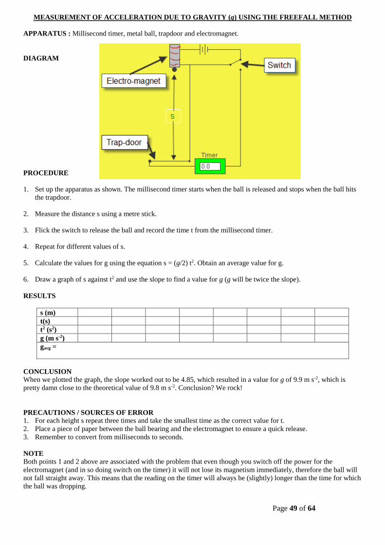
Page 49 of 64
MEASUREMENT OF ACCELERATION DUE TO GRAVITY (g) USING THE FREEFALL METHOD
APPARATUS : Millisecond timer, metal ball, trapdoor and electromagnet.
DIAGRAM
PROCEDURE
1. Set up the apparatus as shown. The millisecond timer starts when the ball is released and stops when the ball hits
the trapdoor.
2. Measure the distance s using a metre stick.
3. Flick the switch to release the ball and record the time t from the millisecond timer.
4. Repeat for different values of s.
5. Calculate the values for g using the equation s = (g/2) t2. Obtain an average value for g.
6. Draw a graph of s against t2 and use the slope to find a value for g (g will be twice the slope).
RESULTS
s (m)
t(s)
t2 (s2)
g (m s-2)
gavg =
CONCLUSION
When we plotted the graph, the slope worked out to be 4.85, which resulted in a value for g of 9.9 m s-2, which is
pretty damn close to the theoretical value of 9.8 m s-2. Conclusion? We rock!
PRECAUTIONS / SOURCES OF ERROR
1. For each height s repeat three times and take the smallest time as the correct value for t.
2. Place a piece of paper between the ball bearing and the electromagnet to ensure a quick release.
3. Remember to convert from milliseconds to seconds.
NOTE
Both points 1 and 2 above are associated with the problem that even though you switch off the power for the
electromagnet (and in so doing switch on the timer) it will not lose its magnetism immediately, therefore the ball will
not fall straight away. This means that the reading on the timer will always be (slightly) longer than the time for which
the ball was dropping.

Page 50 of 64
FORMULA: Since s = ut + ½ (g) t2 and the initial velocity is zero (u=0) then:
FORMULA: s = ½ (g) t2 FUNCTION: y = mx
GRAPH:
Calculation of t2 s
Axes s and t2 labelled points correctly plotted (s , t2) Straight line going through origin
Looking at the formula and the function , we can see that the slope is ½ (g) t2
If we find the slope then we can figure out the gravity g
EXAM QUESTIONS: 2009 (Q1), 2004 (Q1)
SAMPLE : 2004 (Q1) In an experiment to measure the acceleration due to gravity g by a free fall method, a student measured the time t for an object to fall from rest through a distance s. This procedure was repeated for a series of values of the distance s. The table shows the data recorded by the student.
s/cm 30 40 50 60 70 80 90
t/ms 244 291 325 342 371 409 420
(iv) Describe, with the aid of a diagram, how the student obtained the data. (v) Calculate a value for g by drawing a suitable graph. (vi) Give two precautions that should be taken to ensure a more accurate result.
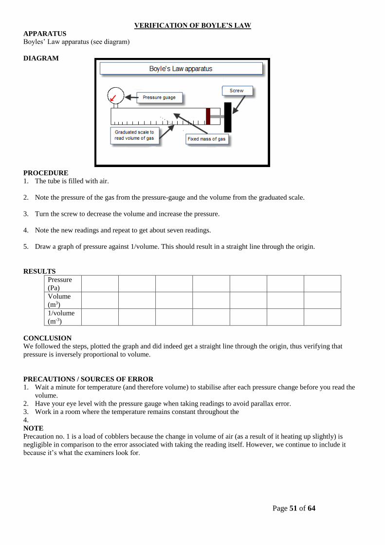
Page 51 of 64
VERIFICATION OF BOYLE’S LAW
APPARATUS
Boyles’ Law apparatus (see diagram)
DIAGRAM
PROCEDURE
1. The tube is filled with air.
2. Note the pressure of the gas from the pressure-gauge and the volume from the graduated scale.
3. Turn the screw to decrease the volume and increase the pressure.
4. Note the new readings and repeat to get about seven readings.
5. Draw a graph of pressure against 1/volume. This should result in a straight line through the origin.
RESULTS
Pressure
(Pa)
Volume
(m3)
1/volume
(m-3)
CONCLUSION
We followed the steps, plotted the graph and did indeed get a straight line through the origin, thus verifying that
pressure is inversely proportional to volume.
PRECAUTIONS / SOURCES OF ERROR
1. Wait a minute for temperature (and therefore volume) to stabilise after each pressure change before you read the
volume.
2. Have your eye level with the pressure gauge when taking readings to avoid parallax error.
3. Work in a room where the temperature remains constant throughout the
4.
NOTE
Precaution no. 1 is a load of cobblers because the change in volume of air (as a result of it heating up slightly) is
negligible in comparison to the error associated with taking the reading itself. However, we continue to include it
because it’s what the examiners look for.

Page 52 of 64
FORMULA: PV = K (Boyle’s Law) We can put it like: FORMULA: P =K/V FUNCTION : y= mx GRAPH:
A straight line through the origin verifies
i.e. P ∝ 1/V.
The slope of the line gives a value
for K if P is in the y-axis and 1/V in the x-axis
mass = slope = y2 – y1
/ x2
– x1
EXAM QUESTIONS: 2013 (Q3), 2003 (Q3)
SAMPLE 2003 (Q3):
In an experiment to verify Boyle’s law, a student measured the volume V of a gas at different values of the pressure p. The mass of the gas was not allowed to change and its temperature was kept constant. The table shows the data recorded by the student. (i) Describe with the aid of a diagram how the student obtained this data. (ii) Draw a suitable graph on graph paper to show the relationship between the pressure of the gas and its volume. (iii) Explain how your graph verifies Boyle’s law. (iv) Describe how the student ensured that the temperature of the gas was kept constant.
p/ kPa 120 180 220 280 320 380 440
V/cm3 9.0 6.0 5.0 4.0 3.5 3.0 2.5

Page 53 of 64
INVESTIGATION OF THE LAWS OF EQUILIBRIUM FOR A SET OF CO-PLANAR FORCES
APPARATUS: Two newton-meters, metre-stick, weights, paperclips, spirit-level, electronic balance
DIAGRAM
PROCEDURE 1. Find and note the centre of gravity of the metre-stick by hanging it from a thread and adjusting the position of the
thread such that the metre-stick is horizontal.
2. Find and note the mass of the metre-stick by weighing it on an electronic-balance.
3. Set up the apparatus as shown and move the weights around until the stick is horizontal and in equilibrium (not
rotating). The newton-metres must be vertical.
4. Record the reading on each newton-metre and the positions on the metre stick of each weight, each newton-metre
and the values of the weights themselves.
RESULTS AND CALCULATIONS FIRST LAW: TOTAL FORCES UP = TOTAL FORCES DOWN
RUN
No.
1st
newton-
metre (N)
2nd
newton-
metre (N)
Total
Upward
Forces (N)
W1
(N)
W2
(N)
Weight of
metre stick
(N)
Total
Downward
Forces (N)
1
2
SECOND LAW: TOTAL MOMENTS CLOCKWISE = TOTAL MOMENTS ANTI-CLOCKWISE
Clockwise Moments
Run
No.
W1
(N)
d1
(m)
W1d1
(Nm)
W2
(N)
d2
(m) W2d2
(Nm)
Wms
dms Wdms
(ms=metre-stick)
Total
moments clock-wise
1
2
Anti-Clockwise Moments
CONCLUSION
We can see from our results that we were able to verify both laws within the margins of experimental error.
SOURCES OF ERROR / PRECAUTIONS
1. Ensure that the Newton balances are vertical and the metre stick is horizontal when readings are taken.
2. Use large weights (i.e. multiples of 1N) to reduce percentage errors.
Run
No.
f3
1st
newton-metre:
(N)
d3
(m)
f3d3
(N m)
f4
2nd
newton-metre:
(N)
d4
(m)
f4d4
(N m)
Total
moments
anti-Clockwise
1
2

Page 54 of 64
NOTES
Why do we have to ensure that all forces are vertical?
Because the moment of a force is defined as being equal to the force multiplied by the perpendicular distance between
the force and the fulcrum. So the easiest way of making sure that forces and distances are perpendicular to each other
is to have the metre-stick horizontal and then all other forces must be perpendicular to this, i.e. vertical.
Do we have to use the extreme left hand side as our reference point?
When calculating the moments, we generally use the 0 cm mark as our fulcrum, and measure all distances from this
point. Strictly speaking we could take any point on the metre stick as our reference point (or fulcrum) but the 0 cm
mark is the easiest.
You should be able to work out the calculations about other points (in the 2002 exam students were asked to calculate
the moments about the 10 cm mark). Apart from all distances now being calculated from the 10 cm mark, the other
change could be that some forces which exerted a clockwise moment about the 0 cm mark may now exert an anti-
clockwise moment about the 10 cm mark.
Watch out!
Setting up the apparatus can be time-consuming and challenging, so you might want to consider the following advice:
As soon as you have everything set-up and balanced, sketch a diagram of it and indicate on it the position and force of
each object.
This should be done as quickly as possible while the apparatus is still stable before anyone bangs against it and brings
it all crashing down.
Once you have all the relevant readings you should fill in the table and work out the calculations – that way if your
results are way off you can double-check them without setting everything up again.
Use large weights
Not only will the large weights reduce the percentage errors associated with the weights themselves, but they will also
help to mask errors associated with the various forces not being horizontal and vertical.
If you are feeling adventurous you could try three or four weights acting down, rather than just two.
FORMULA: FIRST LAW: TOTAL FORCES UP = TOTAL FORCES DOWN
SECOND LAW: TOTAL MOMENTS CLOCKWISE = TOTAL MOMENTS ANTI-CLOCKWISE
GRAPH: None
EXAM QUESTIONS: 2002(Q1), 2007(Q1), 2013 (Q1)
SAMPLE A student investigated the laws of equilibrium for a set of co-planar forces acting on a metre stick. The student found that the centre of gravity of the metre stick was at the 50.4 cm mark and its weight was 1.2 N. (i) How did the student find the centre of gravity? (ii) How did the student find the weight, of the metre stick? (iii) Why is the centre of gravity of the metre stick not at the 50.0 cm mark? (iv) The student applied vertical forces to the metre stick and adjusted them until the metre stick was in equilibrium. How did the student know that the metre stick was in equilibrium? The student recorded the following data. (v) Calculate the net force acting on the metre stick. (vi) Calculate the total clockwise moment about a vertical axis of the metre stick. (vii) Calculate the total anti-clockwise moment about a vertical axis of the metre stick. (viii) Use these results to verify the laws of equilibrium
position on metre stick/cm 11.5 26.2 38.3 70.4 80.2
magnitude of force/N 2.0 4.5 3.0 5.7 4.0
direction of force down up down up down

Page 55 of 64
INVESTIGATION OF THE RELATIONSHIP BETWEEN PERIODIC TIME AND LENGTH FOR A
SIMPLE PENDULUM AND HENCE CALCULATION OF g
APPARATUS
Pendulum bob, split cork, ruler, string and timer
DIAGRAM
PROCEDURE
1. Place the thread of the pendulum between two halves of a cork or
between two coins and clamp to a stand.
2. Set the length of the thread at one metre (from the bottom of the cork or coins to the centre of the bob).
3. Set the pendulum swinging through a small angle (<10°).
4. Measure the time t for thirty complete oscillations.
5. Divide this time t by thirty to get the periodic time T.
6. Repeat for different lengths of the pendulum.
7. Draw a graph of T2
against length l and use the slope to calculate a value for g ( g = 4π2/slope).
RESULTS
l (m)
time for 30 oscillations (s)
time for 1 oscillation (s)
T2 (s2)
g
gavg
CONCLUSION
We got a value for acceleration due to gravity of 9.7 m s-2, which compares favourably with the theoretical value of
9.8
m s-2. We therefore conclude that the theory may well be correct.
SOURCES OF ERROR / PRECAUTIONS
1. Measuring from the bottom of the split-cork to the centre of the bob.
2. Do not cause the pendulum to swing through an angle greater than 10 degrees.
3. Ensure that the pendulum swings in one plane only - avoid circular movements.
4. Use a long pendulum as much as possible to minimise percentage errors associated with measuring the
length and also the time.

Page 56 of 64
What happens acceleration in Simple Harmonic Motion?
Recap
In linear motion, acceleration is always constant in direction and magnitude
In SHM, acceleration by its nature is not constant in either direction or magnitude.
Let’s take another look at this.
Consider a Simple Pendulum*
displacement velocity acceleration
Equiplibrium
position
0 max 0
Extreme
position
max 0 max
The aspect which most people find confusing here is that at the extremities the
velocity is zero, while the acceleration is a maximum, whereas at the equilibrium
position the opposite is the case. How can this be?
Answer:
You must think in terms of forces
Acceleration is directly proportional to the force causing it, so if force is a maximum acceleration must be also, and
vice versa. Now let’s look at the diagram in terms of forces.
At the equilibrium point the restoring force on the mass is zero – it’s not being pulled to the left or the right, therefore
the acceleration must be zero, whereas at the extremities the force pulling the mass back in is a maximum, therefore
the corresponding acceleration must also be also be a maximum.
The other point which might cause confusion is velocity being zero at the extreme positions, but remember we came
across this before; when an object is thrown up its instantaneous velocity is zero at the very top, (even though its
acceleration is not zero).
FORMULA: T = gl2 If you square at both sides of the equation, instead of having T ∝ l you will have
T2 ∝ l which is easier than dealing with square roots .
GRAPH:
Values of t(time for a number of oscillations) divided by number of oscillations recorded in order to get T (Period)
labelled T2 vs. l
straight line through the origin
therefore T2 is proportional to l
EXAM QUESTIONS: 2006(Q1), 2008(Q1), 2012 (Q1)
SAMPLE: 2006 (Q1)
In investigating the relationship between the period and the length of a simple pendulum, a pendulum was set up so that it could swing freely about a fixed point. The length l of the pendulum and the time t taken for 25 oscillations were recorded. This procedure was repeated for different values of the length. The table shows the recorded data. The pendulum used consisted of a small heavy bob attached to a length of inextensible string. (i) Explain why a small heavy bob was used. (ii) Explain why the string was inextensible. (iii) Describe how the pendulum was set up so that it swung
freely about a fixed point. (iv) Give one other precaution taken when allowing the pendulum to swing. (v) Draw a suitable graph to investigate the relationship between the period of the simple pendulum and its length. (vi) What is this relationship? (vii) Justify your answer.
l/cm 40.0 50.0 60.0 70.0 80.0 90.0 100.0
t/s 31.3 35.4 39.1 43.0 45.5 48.2 50.1

Page 57 of 64
TO MEASURE THE SPEED OF SOUND IN AIR
APPARATUS Graduated cylinder, resonance tube open at both ends, tuning forks of known frequency, metre stick, digital callipers
DIAGRAM
PROCEDURE 1. Set up the apparatus as shown in the diagram
2. Strike one of the tuning forks on a block of wood and hold it over the resonance tube.
3. Move the inner-tube slowly until the first loud resonant sound is heard.
4. Measure the distance from the top of the resonance tube to the top of the water (l ). This is approximately one
quarter of the wavelength.
5. Measure the inner-diameter of the resonance tube (d ) using the digital callipers.
6. Note the frequency of the tuning fork; this corresponds to the frequency of the vibrating air column in the
resonance tube.
7. The wavelength of sound is calculated using the formula: c = 4f (l+0.3d)
8. Repeat the procedure with tuning forks of different frequencies. Tabulate the results and get an average value for
the speed of sound in air.
RESULTS
Frequency
(Hz)
Length
(m)
c = f (4l)
(m/s)
diameter d
(m)
0.3 d
(m)
c = 4f(l+0.3d)
(m s-1)
Caverage =
CONCLUSION
We got an average value for the speed of sound to be 300 m s-1, which compares none too favourably with the
theoretical answer of 343 m s-1. But given that the answer is temperature dependent, it may well be the case that we
did our experiment perfectly, but just happened to be a corner of the lab which was at -50 0C.
PRECAUTIONS
1. Ensure that your eye is level with the top of the tube when measuring the length to avoid parallax error.
2. Start with the inner tube fully in the water and slowly raise it so that you don’t get a harmonic by mistake.
3. Repeat your efforts to find the loudest resonance position for each tuning fork. Take the average of the attempts.

Page 58 of 64
So where does the formula c = 4f(l+0.3d) come from?
From our notes we know that for a standing wave the length from node to anti-node is one quarter of the wavelength.
Length from node to anti-node is = /4
Now it’s not at all obvious from this diagram that the wave shape is merely a mathematical representation of the
relative size of the disturbance of the air molecules, but that’s what it is. On the left hand side (the node) there is
almost no disturbance, while on the right hand side (the anti-node) there is maximum disturbance.
Now this is all fine in theory, but in practice we have a 3-dimensional tube, and it turns out that the maximum
displacement of the air molecules is not just at the top of the pipe, but a little outside it. This extra distance is
approximately 0.3 times the diameter.
In this case that means
(Length of tube plus correction term) = /4
= 4 (Length of tube plus correction term)
= 4 (l + 0.3d)
Now we know c = f
c = f [4 (l + 0.3d)]
c = 4f (l + 0.3d)
Important lesson on how to be a good scientist:
We can ignore the small correction term in order to give us a rough idea of what L should be:
c = f c = f (4L ) 340 = 4(f)(L) L = 340 / 4 (f)
Now check this each time before you put a value for L into your table.
FORMULA: c = 4f (l+0.3d)
We can put it like:
FORMULA: l = (c/ 4f) - 0.3d FUNCTION: y =mx + C
Looking at the formula it’s straight line but NOT going through origin where
y= l , x= 1/f, C= - 0.3d , slope=c/4
GRAPH: straight line but NOT going through origin . To get the speed of sound in air (c) through the
graph, you only need to find the slope and then multiplying by 4, as the slope=c/4
EXAM QUESTIONS: 2006(Q3)
SAMPLE: 2006 (Q3)
A cylindrical column of air closed at one end and three different tuning forks were used in an experiment to measure the speed of sound in air. A tuning fork of frequency f was set vibrating and held over the column of air. The length of the column of air was adjusted until it was vibrating at its first harmonic and its length l was then measured. This procedure was repeated for each tuning fork. Finally, the diameter of the column of air was measured. The following data was recorded. Diameter of column of air = 2.05 cm. (ii) Describe how the length of the column of air was adjusted. (iii) Describe how the frequency of the column of air was measured. (iv) Describe how the diameter of the column of air was measured. (v) How was it known that the air column was vibrating at its first harmonic? (vi) Using all of the data, calculate the speed of sound in air.
f/Hz 512 480 426
l/cm 16.0 17.2 19.4

Page 59 of 64
INVESTIGATION OF THE VARIATION OF FUNDAMENTAL FREQUENCY OF A STRETCHED
STRING WITH LENGTH
APPARATUS: Sonometer, newton-meter, tension key, signal generator, u-magnet
DIAGRAM
PROCEDURE
1. Set up as shown on the diagram.
2. Fix the tension at a constant value.
3. Place the bridges as far apart as possible and measure the length of the wire l between the bridges with a metre
stick.
4. Slowly increase the applied a.c. frequency from 0 Hz until the paper-rider vibrates the most.
5. Note the value of this (fundamental frequency) and the length of the wire.
6. Repeat this procedure for different lengths of wire by varying the distance between the bridges.
7. Record the measurements in a table.
8. Plot a graph of frequency f against 1/length.
RESULTS
f (Hz)
l (m)
1/l (m-1)
CONCLUSION
We obtained a straight line through the origin which verifies that frequency is inversely proportional to the length.
PRECAUTIONS / SOURCES OF ERROR
1. Determining exactly where the resonance point is can be tricky so for each length repeat a few times and get an
average.
2. Avoid parallax errors when using a metre stick to measure the length of the wire.

Page 60 of 64
NOTES
1. The Signal Generator Instead of using the signal-generator and U-magnet, you could just use a tuning fork to generate a vibration of a
set frequency (set it vibrating and then stand it either on the sonometer or on one of the bridges). You then vary
the position of the second bridge until you reach resonance. In theory this is simpler; in practice it is much more
difficult to detect the resonance position because the string doesn’t vibrate sufficiently.
You may find the Signal Generator cutting out quite often if you have the current (Amplitude setting) up quite
high, so if you need a high current just use at that setting for as briefly as possible).
If you do go with the signal generator in the exam, you must remember to include the magnet also.
2. The paper rider If a paper rider is used to locate resonance, place it mid-way between the bridges.
Keep the paper rider as light as possible. Use a small piece of cellotape to hold the paper in the form of a loop.
A short length of drinking straw can also be used as a very light rider. This rider can be moved along the string to
detect the positions of nodes and antinodes when the string is vibrating at resonance.
3. Instead of using a newton-metre and a tension-control key you could use weights which hang off of one end.
4. Wear safety goggles in case the sonometer wire snaps.
FORMULA:
T
lf
2
1 FUNCTION: y = mx
GRAPH:
labelled f vs. 1/L straight line through the origin
therefore f 1/L
EXAM QUESTIONS: 2004(Q3), 2012 (Q3)
SAMPLE: 2012(Q3)
In an experiment to investigate the variation of the fundamental frequency f of a stretched string with its length l, the following data were recorded. (i) How was the data obtained? (ii) Using the data, draw a suitable
graph on graph paper to show the relationship between the fundamental frequency of the stretched string and its length.
(iii) The fundamental frequency of a stretched string depends on factors other than its length Name on these factors and give its relationship with the fundamental frequency. (iv) If you were doing an experiment to establish the relationship between the fundamental frequency of a stretched
string and this other factor, how would you obtain the relevant data?
f/Hz 95 102 114 126 141 165 194 232
l/m 0.603 0.553 0.503 0.453 0.403 0.353 0.303 0.253

Page 61 of 64
INVESTIGATION OF THE VARIATION OF FUNDAMENTAL FREQUENCY OF A STRETCHED
STRING WITH TENSION
APPARATUS
Sonometer, newton-meter, tension key, signal generator, u-magnet
DIAGRAM
PROCEDURE
1. Set up as shown on the diagram.
2. Fix the length at a constant value.
3. Set the tension to a low value.
4. Slowly increase the applied a.c. frequency from 0 Hz until the paper-rider vibrates the most.
5. Note the value of this frequency and the tension on the wire.
6. Repeat this procedure for different tensions by varying the tension-control key.
7. Record the measurements in a table.
8. Plot a graph of frequency f against the square root of tension.
RESULTS
f (Hz)
T (N)
T (N1/2)
CONCLUSION
A straight line through the origin will verify that frequency is proportional to the square root of tension.
PRECAUTIONS / SOURCES OF ERROR
Determining exactly where the resonance point is can be tricky so for each tension repeat a few times and get an
average.

Page 62 of 64
*The decibel adjusted scale dB(A) is used because it is adapted to the ear’s frequency response.
A sound gets louder if the sound intensity increases.
However it can get a lot more complicated; if the frequency were adjusted while the sound intensity remained
constant, we would also think that the sound had gotten louder (or quieter), even though a machine would detect no
increase in loudness.
This is because we are more sensitive to some frequencies than others.
So instead of just measuring decibels, we must also bear in mind the frequency involved; the units used to indicate this
new quantity are decibel adjusted (dBA).
A baby’s cry contains frequencies corresponding to the most sensitive part of the human ear’s frequency range (we are
most sensitive to sounds between 2000 Hz and 4000Hz)This means that sounds at these frequencies seem louder than
sounds at other frequencies. This is because the natural frequency of the main bone in the ear is about 3kHz.
*The speed of sound of sound in a solid is greater than in a liquid, which in turn is greater than that for a gas Remember the Cowboys in the Westerns listening for the sound of an on-coming train by putting their ear to the rail-
track?
*The loudness of a note depends upon the amplitude of the sound wave
Loudness also depends upon the sensitivity of the listener; we are more sensitive to some frequencies than others – see
the dBA.
*Harmonics and Overtones The concept of overtones is usually used in conjunction with musical instruments, which emit a number of multiples
all at the same time, whereas harmonics may refer to just a single multiple being sounded at a given time.
Harmonics in a pipe open at one end Harmonics in a pipe open at both ends
*Quality
The quality of a note depends upon the number of overtones present in the note
It also depends upon the relative strengths of the different overtones present.
In practice, when a musical instrument emits a given note (corresponding to a certain frequency), it will also emit a
number of overtones, but at lower strengths.
Different instruments emit different combinations of overtones, and at different strengths.
FORMULA:
T
lf
2
1 FUNCTION: y = mx
GRAPH:
labelled f vs. T straight line through the origin
therefore f T
EXAM QUESTIONS: 2002(Q3), 2009 (Q3)

Page 63 of 64
MEASUREMENT OF THE WAVELENGTH OF MONOCHROMATIC LIGHT
APPARATUS
Laser, diffraction grating (600 lines per mm), 2 metre sticks.
DIAGRAM
PROCEDURE
1. Clamp a metre stick horizontally in a stand.
2. Allow the laser beam to hit the metre stick normally (at 90°).
3. Move the metre stick sideways until the spot is on the 50 cm mark.
4. Place the grating between the laser and the metre stick, at right angles to the beam.
5. Observe the interference pattern on the metre stick – a series of bright spots.
6. Calculate the mean distance x between the centre (n=1) bright spot and the first (n =1) bright spot on both sides of
centre.
7. Measure the distance D from the grating to the metre stick.
8. Calculate θ using tan θ = x/D.
9. Calculate the distance d between the slits, using d =1/N, where N is the number of lines per metre on the grating.
10. Calculate the wavelength λ using nλ = dsinθ.
11. Repeat this procedure for different values of n and get the average value for λ.
RESULTS
n x (m) D (m) θ λ
CONCLUSION
We got a value of 7.10 × 10⁻⁷ m, which sits nicely in the accepted range of 620 – 750 nm for red light.
SOURCES OF ERROR / PRECAUTIONS
1. The diffraction grating may not have been exactly at right angles to the beam of light; x should be the same on
both sides. Measure x on both sides of the n = 0 position and take the average of the two readings. To reduce the
percentage error further just measure the total distance between both points and divide by 2
2. Determining the exact middle of the dot on the screen was difficult (repeat and get an average)

Page 64 of 64
FORMULA: n = d sin GRAPH:none EXAM QUESTIONS: 2004(Q2), 2006(Q2), 2008(Q3), 2011(Q3) SAMPLE: 2008 (Q3) In an experiment to measure the wavelength of monochromatic light, a diffraction pattern was produced using a diffraction grating with 500 lines per mm. The angle between the first order images was measured. This was repeated for the second and the third order images. The table shows the recorded data: (i) Draw a labelled diagram of the
apparatus used in the experiment. (ii) Explain how the first order images were identified. (iii) Describe how the angle between the first order images was measured. (iv) Use the data to calculate the wavelength of the monochromatic light.
2004(Q2)
In an experiment to measure the wavelength of monochromatic light, the angle θ between a central bright image (n = 0) and the first and second order images to the left and the right was measured. A diffraction grating with 500 lines per mm was used. The table shows the recorded data.
n 2 1 0 1 2
θ /degrees 36.2 17.1 0 17.2 36.3
(i) Describe, with the aid of a diagram, how the student obtained the data. (ii) Use all of the data to calculate a value for the wavelength of the light. (iii) Explain how using a diffraction grating with 100 lines per mm leads to a less accurate result. (iv) The values for the angles on the left of the central image are smaller than the corresponding ones on the right.
Suggest a possible reason for this.
Angle between first order images
Angle between second order images
Angle between third order images
34.20 71.60 121.60