learning and model validation - sfu.cakkasa/chokasa_res_revised4.pdf · learning and model...

LEARNING AND MODEL VALIDATION

IN-KOO CHO AND KENNETH KASA

Abstract. This paper studies adaptive learning with multiple models. An agent oper-ating in a self-referential environment is aware of potential model misspecification, andtries to detect it, in real-time, using an econometric specification test. If the currentmodel passes the test, it is used to construct an optimal policy. If it fails the test, anew model is selected. As the rate of coefficient updating decreases, one model becomesdominant, and is used ‘almost always’. Dominant models can be characterized using thetools of large deviations theory. The analysis is used to address two questions posed bySargent’s (1999) Phillips Curve model.

JEL Classification Numbers: C120, E590

If only good things survive the tests of time and practice, evolution produces intelligent design. –Sargent (2008, p.6)

1. Introduction

This paper offers fresh insight into an age-old question - How should policymakersbalance theory and empirical evidence? We study one particular approach to answeringthis question. It consists of the following four-step trial-and-error strategy: (1) An agententertains a competing set of models, M, called the ‘model class’, each containing acollection of unknown parameters. The agent suspects that all his models are misspecified;(2) As a result, each period the agent tests the specification of his current model; (3) Ifthe current model survives the test, the model is updated and used to formulate a policyfunction, under the provisional assumption that the model will not change in the future,and (4) If the model is rejected, the agent experiments by selecting a new model from M.We refer to this combined process of estimation, testing, and selection as model validation.Our goal is to characterize the dynamics of this model validation process.

Our paper builds on the previous work of Sargent (1999). Sargent compares two alter-native histories of the rise and fall of postwar U.S. inflation. These histories differ in theroles played by theory and empirical evidence in macroeconomic policy. According to the“Triumph of the Natural Rate Hypothesis”, inflation was conquered by a Central Bankthat listened to theorists. Theorists convinced the Bank to incorporate the public’s expec-tations into its model. According to the “Vindication of Econometric Policy Evaluation”,inflation was instead conquered by a Central Bank that adapted a simple reduced formstatistical model to evolving conditions. Our model validation approach blends elementsof both the ‘Triumph’ story and the ‘Vindication’ story. According to model validation,

Date: June, 2014.We thank the editor and three anonymous referees for helpful comments. We are also grateful to JimBullard, Steve Durlauf, Lars Hansen, Seppo Honkapohja, Albert Marcet, and Tom Sargent for helpfuldiscussions. Financial support from the National Science Foundation (ECS-0523620, SES-0720592) isgratefully acknowledged.

1

2 IN-KOO CHO AND KENNETH KASA

the role of theorists is to convince policymakers to add (good) models to M. The role ofeconometricians is to then evaluate these models empirically. We argue this blending oftheory and evidence is reasonably descriptive of actual practice. Policymakers rarely trustmodels that have obvious data inconsistencies. However, good policymakers know that itis all too easy to make bad models fit the data, so it is important that models be basedon sound economic theory, even if there is disagreement about the right theory. Despiteits descriptive realism, the normative implications of model validation are not well under-stood, and so one of our goals is to shed light on the conditions under which it producesgood outcomes, and just as important, when it does not. Given the assumed endogeneityof the data-generating process, this kind of question has been neglected by the traditionaleconometrics literature.

1.1. A Motivating Example. It is useful to begin by illustrating model validation inaction. This will highlight both its strengths and its potential weaknesses. We do thisby revisiting Sargent’s (1999) Conquest model. Sargent studied the problem of a CentralBank that wants to minimize a quadratic loss function in unemployment and inflation,E(u2

n+π2n), but is unsure about the true model. The Bank posits a reduced form regression

model of the form, un = γ0 +γ1πn, and then tries to learn about it by adaptively updatingthe parameter estimates using a (discounted) least-squares algorithm. The Bank’s optimalinflation target, xn = −γ0,nγ1,n/(1+ γ2

1,n), evolves along with its parameter estimates. Un-beknownst to the Bank, the true relationship between un and πn is governed by a NaturalRate model, in which only unanticipated inflation matters, un = u∗ − θ(πn − xn) + v1,n,where u∗ is the natural rate of unemployment, and πn − xn = v2,n represents unexpectedinflation. The inflation shock, v2,n, is i.i.d. Notice that the Bank’s model is misspecified,since it neglects the role of expectations in shifting the Phillips Curve. Evolving expecta-tions manifest themselves as shifts in the estimated intercept of the reduced form PhillipsCurve.

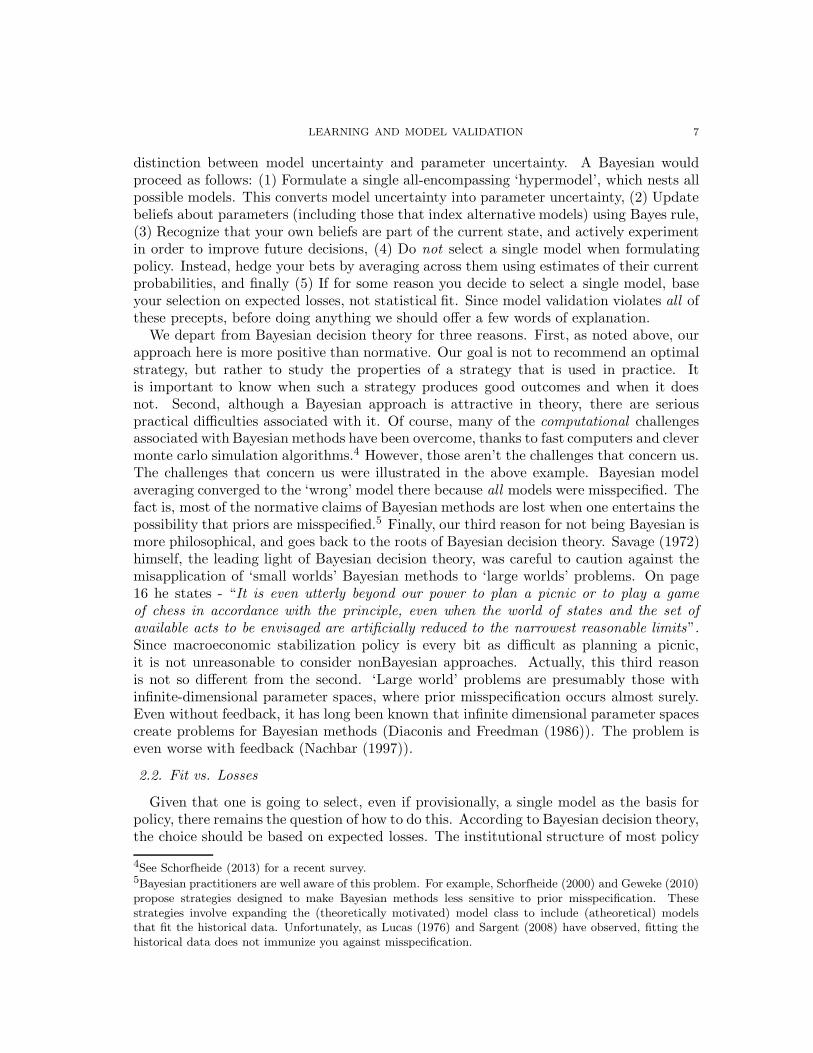
The top left panel of Figure 1 illustrates the resulting inflation dynamics, using thesame parameter values as Sargent (1999).

500 1000 1500 2000 2500−2

0

2

4

6Inflation in Sargents Model

500 1000 1500 2000 2500−2

0

2

4

6Inflation with Recursive t−test

500 1000 1500 2000 2500−2

0

2

4

6Inflation with Model Averaging

500 1000 1500 2000 2500−2

0

2

4

6Inflation with Model Validation

Figure 1. Model Averaging vs. Model Validation in Sargent’s Conquest Model

LEARNING AND MODEL VALIDATION 3

The striking feature here is the recurring cycle of gradually rising inflation, and occa-sional sharp inflation stabilizations. As noted by Cho, Williams, and Sargent (2002), thiscycle represents the interplay between the model’s mean dynamics and its escape dynam-ics. The mean dynamics reflect the Central Bank’s efforts to eliminate systematic forecasterrors. These errors are eliminated once inflation reaches its Self-Confirming Equilibrium(SCE) value of 5%. The escape dynamics are more exotic. At the SCE, the Bank’s beliefsare free to wander in any direction, and when sequences of positively correlated inflationand Phillips Curve shocks occur, they cause the Bank to revise downward its PhillipsCurve slope estimate, and therefore, its inflation target. Since in truth there is no ex-poitable trade-off, these inflation reductions produce further downward revisions, and theprocess feeds on itself until inflation reaches the Ramsey outcome of zero inflation. Fromhere, with no further changes in the inflation target, the Bank begins to rediscover thePhillips Curve, due to the presence of inflation shocks acting within the model’s naturalrate structure. This produces a gradual pull back to the SCE.

A natural question at this point is - To what extent is the Central Bank really learninganything here? True, it’s revising estimates of a model in light of new data, but in practicepolicymakers spend most of their time looking for new and improved models, not refiningestimates of a given model. In Sargent (1999), the Central Bank never really evaluates thePhillips Curve as a theoretical model of inflation and unemployment; it merely reconsidersthe strength of an unquestioned trade-off. Evidently, this produces a bad outcome, as theBank repeatedly succumbs to the temptation to try to exploit the Phillips Curve.

The remaining three panels of Figure 1 therefore explore the consequences of moresophisticated learning strategies, assuming the Bank confronts the same sequence of ex-ogenous shocks. The top right panel assumes the Bank engages in a traditional process ofhypothesis testing. In particular, suppose the Bank entertains the possibility that there isno trade-off. In response, the Bank decides to sequentially test the hypothesis that γ1 = 0,and if the hypothesis is not rejected, it sets the inflation target to zero. Clearly, this makesvirtually no difference, other than a slight delay in the return to the SCE. The fact is,there is a correlation between inflation and unemployment, albeit not an exploitable one,and this correlation causes the Bank to quickly reject the null hypothesis that γ1 = 0.The problem, of course, is that the Bank’s model is subject to a fundamental misspecifica-tion, based on a misinterpretation of the role of the public’s expectations in the inflationprocess. To break out of its inflation cycle, the Bank must consider other models.

The bottom two panels of Figure 1 assume the Bank has two models: (1) the statisticalPhillips Curve, as before, and (2) a vertical Phillips Curve, un = γ0+εn. The second modelcalls on the Bank to always set target inflation to zero. The problem is that it is not surewhich model is correct. The lower left panel assumes the Bank responds to this uncertaintyin traditional Bayesian fashion, by averaging across the two models. That is, it assigns aprior to the two models, updates its prior as new data come in, and each period sets itsinflation target as the current probability weighted average of the target recommended byeach of the two models, which is optimal given its quadratic loss function.1 The red lineplots the recursively estimated probability of the Natural Rate model. The initial prior isassumed to be (.5, .5), with parameter values initialized at their respective SCE values.

1Note, the Bank is not fully complying with an optimal Bayesian strategy, since we assume it does notactively experiment.


Although early on the Bank has confidence for awhile in the Natural Rate Hypothesis, iteventually comes to believe that the misspecified Phillips Curve is the correct model, andit never regains any confidence in the Natural Rate Hypothesis. How can this be? Howcould a Bayesian ever settle on the wrong model when the true model is in the support ofhis prior? The usual Bayesian consistency theorems do not apply here because the verticalPhillips Curve does in fact contain a subtle misspecification, since the data continue tobe generated by Sargent’s expectations-augmented Phillips Curve, in which one of theshocks is unexpected inflation. This introduces feedback from the Bank’s policy to theactual data-generating process, which the vertical Phillips curve neglects. In contrast,the statistical Phillips curve exploits this feedback to improve its relative fit, and so iteventually drives out the vertical Phillips Curve.2

The lower right panel of Figure 1 illustrates what happens under model validation.The Bank has the same two models as before, but now selects just one model whenformulating its inflation target. The selection is based on the outcome of a recursiveLagrange Multiplier test (discussed in more detail below). The current model continues tobe used as long as it appears to be well specified. If the current model is rejected, a newmodel is randomly selected, with selection probabilities determined by historical relativeforecast accuracy. (The figure uses a logit function with a ‘choice intensity parameter’ of 2).The simulation is initialized by assuming the Bank begins with Sargent’s statistical PhillipsCurve, with parameters set at their SCE values. As before, parameter estimates eventuallyescape from the neighborhood of the SCE, and move toward the Ramsey outcome. InSargent’s analysis, this large and rapid movement does not lead the Bank to reconsiderthe validity of the Phillips Curve. In contrast, under model validation, the escape triggersa rejection of the specification test, and the Bank switches to the vertical Phillips Curve.Once it does so, it ‘never’ goes back, and inflation remains at the Ramsey outcome. Note,the Bank does not rule out the possibility of an expoitable trade-off once it switches tothe vertical Phillips Curve. The vertical Phillips Curve continues to be tested just asthe exploitable Phillips Curve was tested. The difference is that the likelihood of escapeand rejection is orders of magnitude smaller for the vertical Phillips Curve, and so for allpractical purposes the Bank learns not to exploit the Phillips Curve. The analysis in thepaper will explore in detail why some models are more resilient to repeated specificationtesting than others. We shall see that a key part of the story lies in the strength of theirself-referential feedback.

1.2. Lessons. So what lessons have been learned here? First, the comparison betweenmodel validation and recursive t-testing highlights the importance of allowing agents to

2Evans, Honkapohja, Sargent, and Williams (2013) contains a similar result. They consider a standardcobweb model, in which agents average between a time-varying parameter specification, and a constant-parameter specification. They assume the true model has constant parameters, but find that Bayesianmodel averaging often converges to the time-varying parameter model, even when the initial prior putssignificant weight on the true constant parameter model. This occurs when self-referential feedback frombeliefs to outcomes is sufficiently strong. Cogley, Colacito, and Sargent (2007) is also similar. Theyconsider a Central Bank that averages between a Natural Rate model and a statistical Phillips Curve. Intheir model, the Central Bank always learns the true model. Two factors explain the difference: (1) TheirNatural Rate model is not misspecified, as it correctly conditions on expected inflation. This eliminatesone source of feedback. (2) They assume the Bank knows each model’s parameter values, so that policyonly depends on model weights, not parameter estimates. This eliminates the other source of feedback.


entertain multiple models. A statistician might argue that the difference between thestatistical Phillips Curve and the vertical Phillips Curve cannot possibly be relevant, sincethe vertical Phillips Curve is nested within the statistical Phillips Curve. Isn’t there reallyjust one model here? By starting with the more general specification, wouldn’t a goodeconometrician eventually discover the right model? Although this is a valid argumentwhen the data are exogenous and the general model encompasses the true model, it doesnot apply when the data are endogenous and all models are misspecified, e.g., whenalternative models respond differently to underlying feedback in the data. Fully capturingthe intricate feedbacks that exist between macroeconomic policy and time-series data is achallenging exercise, to say the least, and so it is important to devise learning strategiesthat are reliable even when all models potentially misspecify this feedback. Second, thecomparison between model validation and model averaging simply reinforces this point. ABayesian would never commit to a single model on the basis of a hypothesis test. Why nothedge your bets and average? Again, this makes sense when the prior encompasses thetruth, but there is no guarantee it produces good outcomes when priors are misspecified.The above example illustrates the dangers of model averaging with endogenous data andmisspecified models.

Although suggestive, the above simulations are just an example. How, if at all, dothey generalize? As in Sargent (2008) and Fudenberg and Levine (2009), our goal in thispaper is to understand how feedback and experimentation interact to influence macroeco-nomic model selection. Addressing this question poses serious technical challenges. Withendogenous data and multiple models, each with adaptively estimated coefficients, theunderlying state of the economy is of high dimension, and it evolves nonlinearly. Thekey to making this system tractable is to exploit the fact that under certain conditionssubsets of the variables evolve on different time-scales. By appropriately averaging overeach subset, we can simplify the analysis to one of studying the interactions between lowerdimensional subsystems. This is a commonly employed strategy in science, going back to19th century celestial mechanics. Marcet and Sargent (1989) were the first to apply it inthe macroeconomic learning literature.

Our analysis extends the work of Marcet and Sargent (1989). We show that modelvalidation dynamics feature a hierarchy of three time scales. This hierarchy of time-scalespermits us to focus separately on the problems of control, model revision, and modelselection. As in Marcet and Sargent (1989), economic variables evolve on a ‘fast’, calendartime-scale, whereas coefficient estimates evolve on a ‘slow’, model revision time-scale. Thenew element here is that under appropriate assumptions on specification testing, modelselection occurs on a ‘really slow’, model switching time-scale. Model switches are rarehere, because they are triggered by departures from a model’s self-confirming equilibrium,and are therefore ‘large deviation’ events. The fact that each model’s coefficients canbe adapted to fit the data it generates is crucial to this result, and it illustrates a keydifference between specification testing with endogenous data and specification testingwith exogenous data.

We show that model selection dynamics can be approximated by a low dimensionalMarkov chain, in which each model’s coefficients are fixed at their self-confirming values,and the economic data are fixed at the mean of the invariant distribution associated withthese values. In the limit, as the update gain parameter converges to zero, the invariantdistribution of this Markov chain collapses onto a single model. We can identify this model


from its large deviations rate function. Our analysis therefore provides an equilibriumselection criterion for recursive learning models. It can also be interpreted as a refinementof the concept of self-confirming equilibria.

Large deviation methods provide an interesting interpretation of this limiting model.We show that it is the model possessing the largest ‘rate function’. A key result in thetheory of large deviations (Sanov’s theorem) links this rate function to relative entropyand the Kullback-Leibler Information Criterion (KLIC). The KLIC is a pervasive conceptin the econometrics literature on model testing and selection. The relative entropy that isbeing captured by each model’s rate function is the KLIC distance between the probabilitydistribution associated with its SCE and the distribution associated with the closest modelthat triggers a rejection or escape. This extends the results of White (1982) in a naturalway to the case of endogenous data.

The remainder of the paper is organized as follows. Section 2 provides an overviewof some new issues that arise when combining model uncertainty with adaptive learning.Section 3 maps our model validation approach into a standard Stochastic Recursive Al-gorithm. Section 4 uses results from the large deviations literature to characterize modelvalidation dynamics. Section 5 derives explicit expressions for the case of linear Gaussianmodels. These expressions show that feedback is a key determinant of a model’s durability.Section 6 returns to Sargent’s (1999) Conquest model. We first use our large deviationsanalysis to explain the results in Figure 1. We then go on to consider a second example.In this example the Bank is unsure about identification; in particular, whether to imposea Classical or Keynesian identification restriction. Here model validation leads to the‘wrong’ model. Section 7 briefly discusses some related literature, while Section 8 offers afew concluding remarks. An appendix contains proofs of some technical results.

2. Overview

Incorporating multiple models into the learning literature raises a host of new questionsand issues. This section briefly outlines how model validation addresses these issues. Manyof the ingredients are inspired by the discussion in Sims (2002), who visited the world’smajor Central Banks, and described their basic policymaking strategies. Interestingly,these strategies are quite similar. They share the following features: (1) They all usemultiple models, (2) The models have evolved over time in response to both theory anddata, (3) At a given point in time, there is a reliance on a ‘primary model’, and (4) Theprocess itself is decentralized between a professional staff that develops and monitors themodels, and a smaller group of appointed policymakers who make decisions by combiningmodel projections with other (more subjective) data. Sims (2002) goes on to criticizemany of these practices, and advocates a more Bayesian approach to policy. In contrast,we adopt a less normative and more descriptive viewpoint, and seek to characterize theoutcomes produced by this process.

2.1. Why Not Bayesian?

Bayesian decision theory offers an elegant and theoretically coherent methodology fordealing with model uncertainty.3 From a Bayesian perspective, there is no meaningful

3See, e.g., Brock, Durlauf, and West (2007) for an application of Bayesian decision theory to modeluncertainty and macroeconomic policy.


distinction between model uncertainty and parameter uncertainty. A Bayesian wouldproceed as follows: (1) Formulate a single all-encompassing ‘hypermodel’, which nests allpossible models. This converts model uncertainty into parameter uncertainty, (2) Updatebeliefs about parameters (including those that index alternative models) using Bayes rule,(3) Recognize that your own beliefs are part of the current state, and actively experimentin order to improve future decisions, (4) Do not select a single model when formulatingpolicy. Instead, hedge your bets by averaging across them using estimates of their currentprobabilities, and finally (5) If for some reason you decide to select a single model, baseyour selection on expected losses, not statistical fit. Since model validation violates all ofthese precepts, before doing anything we should offer a few words of explanation.

We depart from Bayesian decision theory for three reasons. First, as noted above, ourapproach here is more positive than normative. Our goal is not to recommend an optimalstrategy, but rather to study the properties of a strategy that is used in practice. Itis important to know when such a strategy produces good outcomes and when it doesnot. Second, although a Bayesian approach is attractive in theory, there are seriouspractical difficulties associated with it. Of course, many of the computational challengesassociated with Bayesian methods have been overcome, thanks to fast computers and clevermonte carlo simulation algorithms.4 However, those aren’t the challenges that concern us.The challenges that concern us were illustrated in the above example. Bayesian modelaveraging converged to the ‘wrong’ model there because all models were misspecified. Thefact is, most of the normative claims of Bayesian methods are lost when one entertains thepossibility that priors are misspecified.5 Finally, our third reason for not being Bayesian ismore philosophical, and goes back to the roots of Bayesian decision theory. Savage (1972)himself, the leading light of Bayesian decision theory, was careful to caution against themisapplication of ‘small worlds’ Bayesian methods to ‘large worlds’ problems. On page16 he states - “It is even utterly beyond our power to plan a picnic or to play a gameof chess in accordance with the principle, even when the world of states and the set ofavailable acts to be envisaged are artificially reduced to the narrowest reasonable limits”.Since macroeconomic stabilization policy is every bit as difficult as planning a picnic,it is not unreasonable to consider nonBayesian approaches. Actually, this third reasonis not so different from the second. ‘Large world’ problems are presumably those withinfinite-dimensional parameter spaces, where prior misspecification occurs almost surely.Even without feedback, it has long been known that infinite dimensional parameter spacescreate problems for Bayesian methods (Diaconis and Freedman (1986)). The problem iseven worse with feedback (Nachbar (1997)).

2.2. Fit vs. Losses

Given that one is going to select, even if provisionally, a single model as the basis forpolicy, there remains the question of how to do this. According to Bayesian decision theory,the choice should be based on expected losses. The institutional structure of most policy

4See Schorfheide (2013) for a recent survey.5Bayesian practitioners are well aware of this problem. For example, Schorfheide (2000) and Geweke (2010)propose strategies designed to make Bayesian methods less sensitive to prior misspecification. Thesestrategies involve expanding the (theoretically motivated) model class to include (atheoretical) modelsthat fit the historical data. Unfortunately, as Lucas (1976) and Sargent (2008) have observed, fitting thehistorical data does not immunize you against misspecification.


environments makes this difficult in practice. Policy environments in economics oftenmimic those in the natural sciences, which feature a division of labor between technicians,who build and validate models, and policymakers, who evaluate costs and benefits andmake decisions based (partly) on model projections. The fact is, model builders often haveimperfect knowledge of the objectives and contraints of policymakers, which makes loss-based model selection procedures problematic. Model validation focuses on the problemof the technicians. These technicians blend theory and evidence in an effort to give thebest advice possible to policymakers. It is not too surprising that a separation betweenmodel validation and decision-making can produce bad outcomes. Section 6 provides anexample.6 Perhaps more surprising is the observation that it sometimes does producegood outcomes, as we saw in Figure 1.

2.3. Counterfactuals

The fact that the data-generating process responds to the agent’s own beliefs is a crucialissue even without model uncertainty. It means all the classical econometric results onconvergence and consistency of least-squares estimators go out the window. Developingmethods that allow one to rigorously study the consequences of feedback has been a centralaccomplishment of the macroeconomic learning literature. Evans and Honkapohja (2001)summarize this literature.

When one turns to inference, however, new issues arise. First, the presence of feedbackmeans that we cannot directly apply recent econometric advances in testing and comparingmisspecified models (White (1994)). Although we assume the agent is aware of theseadvances, and tries to implement them, we cannot appeal to known results to studytheir consequences. Second, traditionally it has been assumed that agents are unawareof feedback. Although beliefs are revised in an adaptive and purposeful manner, thisadaptation is strictly passive. This is a reasonable assumption in the context of learningthe parameters of a single model, mainly because one is already confined to a local analysis.With multiple models, however, the distinction between local and global analysis becomesmore important. We depart from tradition here by assuming the agent is aware of feedback,even though he responds to it in a less than optimal manner. In particular, he realizesthat with multiple models he confronts a difficult counterfactual - How would things havebeen different if instead a different model had been used in the past? Fitting a modelto data that was generated while a different model was in use could produce misleadinginferences about the prospects of a given model. For the questions we address, it is notimportant how exactly the agent responds to this counterfactual. What’s important isthat he is aware of its dangers.

2.4. Specification Testing

We assume the agent sticks with a model until sufficient evidence mounts against it.This evidence takes the form of an econometric specification test. It turns out specificationtesting can be embedded within a standard Stochastic Recursive Algorithm. In particular,the orthogonality condition that drives parameter updating can be interpreted as a scorestatistic, or equivalently, a localized likelihood ratio statistic, which can be used as thebasis of a sequential Lagrange Multiplier test. (See, e.g., Chapter 5 of Benveniste, Metivier,

6Kocherlakota (2007) provides more examples of the dangers of basing model selection on model fit.


and Priouret (1990)). When the score statistic exceeds a time-varying theshold tuned tothe environment’s feedback, it indicates that required parameter changes are faster andlarger than specified by the constant gain null hypothesis of gradual parameter drift.7

2.5. Escape Dynamics, Type I Errors, and the Robustness of Self-Confirming Equilibria

We assume for simplicity that each model, when used, has a unique, stable, self-confirming equilibrium. This means that each model, if given the chance, is capable ofpassing the specification test. This does not imply it is the ‘true’ data-generating process.In fact, the entire model class may be misspecified. However, with endogenous data, eachmodel can adapt to fit the data that it itself generates. It is this possibility that wreakshavoc with the application of traditional statistical results.

Although all models are capable of passing the test, they are not all equally likelyto do so on a repeated basis. Some models are more ‘attached’ to their self-confirmingequilibrium, while others are more apt to drift away. Model drift is driven by the fact thatcoefficient estimates drift in response to constant gain updating. We calibrate the testingthreshold so that this kind of normal, gradual, parameter drift does not trigger modelrejection. However, as noted by Sargent (1999), constant gain algorithms also featurerare, but recurrent, ‘large deviations’ in their sample paths. These large deviations can becharacterized analytically by the solution of a deterministic control problem. It is theserare escapes from the self-confirming equilibrium that trigger model rejections. In a sensethen, model rejections here are Type I errors.

The value function of the large deviations control problem is called the ‘rate function’,and as you would expect, it depends sensitively on the tails of the score statistic. InSection 4 we show that as the update gain decreases the model with the largest ratefunction becomes dominant, in the sense that it is used ‘almost always’. This bears someresemblence to results in the evolutionary game theory literature (Kandori, Mailath, andRob (1993)). It also provides a selection criterion for models with multiple stable self-confirming equilbria.

2.6. Experimentation

When a model is rejected we assume the agent randomly selects a new model (whichmay turn out to be the existing model). This randomness is deliberate. It does not reflectcapriciousness or computational errors, but instead reflects a strategic response to modeluncertainty (Foster and Young (2003)). It can also be interpreted as a form of experi-mentation. Of course, macroeconomic policymakers rarely conduct explicit experiments,but they do occasionally try new things. Although the real-time dynamics of model selec-tion naturally depend on the details of the experimentation process, our main conclusionsabout the stability and robustness of self-confirming equilibria do not.

3. A General Framework

Traditional learning models focus on the dynamic interaction between beliefs and ob-served data. Beliefs are summarized by the current estimates of a model’s parameters,

7Another possible response to an excessively large score statistic would be to allow the update gain toincrease. See Kostyshyna (2012) for an analysis of this possibility.


βn ∈ Rd1 , and are updated recursively as follows,

βn = βn−1 + εnG(βn−1, Xn)

where G : Rd1 × Rd2 → Rd1 captures some notion of the model’s fit or performance.In many applications G is determined by least squares orthogonality conditions. The‘gain sequence’, εn dictates how sensitive beliefs are to new information. In stationaryenvironments εn → 0, as each new observation becomes less important relative to theexisting stock of prior knowledge. However, in nonstationary environments it is optimalto keep ε bounded away from zero, and that is the case we consider. For simplicty, weassume it is a constant. The data, Xn ∈ Rd2 , evolve according to a stationary Markovprocess

Xn = F (βn−1, Xn−1, Wn)

where Wn ∈ Rd3 is a vector of exogenous shocks. The function F : Rd1 ×Rd2 ×Rd3 → Rd2

captures the interaction between the agent’s model, his beliefs, and the underlying envi-ronment. The key feature here is the dependence of F on β. This makes the environment‘self-referential’, in the sense that the underlying data-generating process depends on theagent’s beliefs.

Most of the existing learning literature has been devoted to studying systems of thisform. This is not an easy task, given that it represents a nonlinear, dynamic, stochasticsystem. Until recently attention primarily focused on long-run convergence and stabilityissues. A more recent literature has focused on sample path properties. As noted earlier,the key to making the analysis feasible is to exploit the fact that βn and Xn operate ondifferent time-scales, due to the presence of ε in the parameter update equations. As ε → 0,βn evolves more and more slowly relative to Xn. This allows us to decouple the analysisof the interaction between beliefs and outcomes into two separate steps: (1) First examinethe long-run average behavior of the data for given beliefs, X(β), and then substitute thisaveraged behavior into the belief update equations, which then produces an autonomousequation for βn. In the economics literature, this ‘mean ODE approach’ was pioneered byMarcet and Sargent (1989). Evans and Honkapohja (2001) provide a detailed summary.

Model validation represents a natural extension of these ideas. When agents entertainmultiple candidate models, one can simply index them by a discrete model indicator,sn ∈ M, and then think of sn as just another parameter. However, in contrast to Bayesiandecision theory, the agent is assumed to display a greater reluctace to revise beliefs aboutsn than about other parameters.8 Our maintained assumption is that the agent believesthere to be a single best model within M, and the goal is to find it, while at the sametime balancing the ongoing pressures of meeting control objectives.

Technically, the key issue is to show that specification testing introduces a third time-scale, in the sense that the evolution of sn can itself be decoupled from the evolution ofeach model’s parameter estimates. So, to begin the analysis, we just need to augment theupdating and data processes as follows:

βin = βi

n−1 + εGi(sn−1, βn−1, Xn) ∀i ∈ M (3.1)Xn = F (sn−1, βn−1, Xn−1, Wn) (3.2)

8We thank an anonymous referee for providing this interpretation. Note, this kind of distinction betweenmodels and parameters is also present in Hansen and Sargent’s (2008, chpt. 18) work on robust learning.


The first equation implies the parameter estimates of each model will in general dependon which model is currently being used. This reflects our assumption that each modelis continuously updated, even when it is not being used to make decisions. The secondequation makes clear that now the economy is operating with a new layer of self-reference.Not only does policy potentially depend on beliefs about a particular model, but also onthe model itself. The feedback from beliefs to the actual DGP is case specific, and can bequite complex and highly nonlinear. Fortunately, all we need is the following assumption.

Assumption 3.1. For fixed (βn, sn) = (β, s), the state variables Xn possess a uniqueinvariant distribution.

Our analytical methods rely heavily on the ability to ‘average out’ fluctuations in Xn

for given values of the model coefficients and model indicator. Assumption 3.1 guaranteesthese averages are well defined. Evans and Honkapohja (2001) provide sufficient conditions.To facilitate the analysis, we further assume that the set of feasible coefficients for eachmodel satisfies some regularity conditions.

Assumption 3.2. Let Bi be the set of all feasible coefficients for model i. We assumethat Bi is compact and convex.

This compactness assumption can be interpreted as a priori knowledge about the DGP.Although the agent does not know the precise values of the coefficients, he can rule out out-rageously large coefficients. These bounds can be enforced algorithmically by a ‘projectionfacility’ (see, e.g., Kushner and Yin (1997)). Convexity is mainly a technical assumption,designed to address the learning dynamics along the boundary of the parameter space.

As noted earlier, we assume the agent operates under a ‘if it’s not broke, don’t fix it’principle, meaning that models are used until they appear to be misspecified, as indicatedby a statistical specification test. The test is performed recursively, in real-time, and forthe same reasons that past data are discounted when computing parameter estimates,we assume estimates of the test statistic, θn ∈ R1

+, are updated using a constant gainstochastic approximation algorithm,

θn = θn−1 + εα[Q(sn−1, βn−1, Xn) − θn−1] (3.3)

where Q(sn−1, βn−1, Xn) is the time-n value of the statistic. Averaging by letting α > 0 isimportant, as it prevents single isolated shock realizations from triggering model rejections.At the same time, letting α < 1 is convenient, since otherwise θn evolves more slowly thanβn, making the test statistic depend on the history of the coefficient estimates, rather thanjust their current magnitudes. This would complicate the derivation of the large deviationproperties of the test statistic.

Finally, if |M| = m, then the model indicator parameter, sn, follows an m-state Markovchain that depends on the current value of the test statistic relative to an evolving testthreshold, θn,

sn+1 = I(θn≤θn) · sn + (1 − I(θn≤θn)) · Πn+1 (3.4)

where I is an indicator function, and Πn is a post-rejection model selection distributionwith elements πi

n, i = 1, 2, · · ·m. The only restriction that must be placed on Πn isthat it have full support ∀n. In practice, one would expect Πn to evolve, and to reflectthe historical relative performance of the various models, with better performing models


receiving higher weights. Our analysis permits this, as long as the elements of Πn remainstrictly positive. In our simulations we use the logit function,

πin =

e−φωi,n

∑mj=1 e−φωj,n

where ωi,n is an estimate of model-i’s one-step ahead forecast error variance, and φ is a‘choice intensity’ parameter. As φ increases, the agent is less prone to experiment.

Equations (3.1)-(3.4) summarize our model validation framework. Our goal is to un-derstand the asymptotic properties of this system (as ε → 0), with a special focus on theasymptotic properties of the model selection parameter, sn.

3.1. Mean ODEs and Self-Confirming Equilibria. Notice the Xn vector on the right-hand side of (3.1) corresponds to the actual law of motion given by (3.2), which dependson both the current model and the agent’s control and estimation efforts. This makesthe agent’s problem self-referential. It also makes analysis of this problem difficult. Tosimplify, we exploit a two-tiered time-scale separation, one between the evolution of thedata, Xn, and the evolution of each model’s coefficient estimates, βi

n, and another betweenthe evolution of the coefficient estimates and the rate of model switching, sn. A key conceptwhen doing this is the notion of a mean ODE, which is obtained by following four steps:(1) Substitute the actual law for Xn given by (3.2) into the parameter update equationsin (3.1), (2) Freeze the coefficient estimates and model indicator at their current values,(3) Average over the stationary distribution of the ‘fast’ variables, Xn, which exists byAssumption 1, and (4) Form a continuous time interpolation of the resulting autonomousdifference equation, and then obtain the mean ODE by taking limits as ε → 0.

Assumption 3.1 assures us that this averaging is well defined. We also need to makesure it is well behaved. To facilitate notation, write the update equations for model-i asfollows. Let P k

β,s(Xn+k ∈ ·|Xn) be the k-step transition probability of the data for fixedvalues βn = β and sn = s, and let Γβ,s(dξ) = limk→∞ P k(·) be its ergodic limit. Definethe function

gi(s, βi) =∫

Gi(s, βi, ξ)Γβ,s(dξ) (3.5)

We impose the following regularity condition on g(·),

Assumption 3.3. For all i and s, gi(s, βi) is a Lipschitz continuous function of βi.

Continuity is essential for our averaging strategy to work. Note that since the parameterspace is bounded, Assumption 3.3 implies g is bounded.

A subtlety arises here from model switching. We assume that after a model is rejectedit continues to be fit to data generated by other models. As a result, there is no guaranteethat while a model is not being used its coefficient estimates remain in the neighborhoodof its self-confirming equilibrium. Instead, its estimated coefficients tend to gravitateto some other self-confirming equilibrium, one that satisfies the model’s orthogonalitycondition given that data are being generated by another model. However, as long asmodel rejections occur on a slower time-scale than coefficient updating, we can apply thesame averaging principle as before, the only difference is that now for each model we obtaina set of m mean ODEs (the next section contains a formal proof),

βis = gi(s, βi

s) s = 1, 2, · · ·m (3.6)


where βis denotes model i’s coefficient estimates given that model s is generating the data.

Note that when model s 6= i generates the data, its coefficent estimates influence model-i’smean ODE. This is because the rate of coefficient updating is assumed to be the same forall models. A self-confirming equilibrium for model-i, β∗

i,s, is defined to be a stationarypoint of the mean ODE in (3.6), i.e., gi(s, β∗

i,s) = 0. Note that in general it depends onwhich model is generating the data. To simplify the analysis, we impose the followingassumption

Assumption 3.4. Each model i = 1, 2, · · · , m has a unique vector of globally asymptoti-cally stable Self-Confirming Equilibria, β∗

i,s, s = 1, 2, · · · , m

This is actually stronger than required. All we really need is global asymptotic stabilityof β∗

i,i, ∀i. This guarantees that after a period of disuse, each model converges back to itsown unique self-confirming equilibrium. If this weren’t the case, then the problem wouldlose its Markov structure. However, given the boundedness we’ve already imposed onthe parameter space, we don’t need to worry too much about how a model’s coefficientestimates behave while other models generate the data. Finally, note that if a model’s ownself-confirming equilibrium is unstable, one would expect its relative use to shrink rapidlyto zero as ε → 0, since in this case model rejections are not rare events triggered by largedeviations. Instead, they occur rapidly in response to a model’s own mean dynamics.

3.2. Model Validation. There is no single best way to validate a model. The rightapproach depends on what the model is being used for, and the nature of the relevantalternatives. In this paper we apply a Lagrange Multiplier (LM) approach. LM tests canbe interpreted as Likelihood Ratio tests against local alternatives, or as first-order approx-imations of the Kullback-Leibler Information Criterion (KLIC). Their defining feature isthat they are based solely on estimation of the null model, and do not require specificationof an explicit alternative. As a result, they are often referred to as misspecification tests.Benveniste, Metivier, and Priouret (1990) (BMP) outline a recursive validation procedurebased on LM testing principles. Their method is based on the observation that the inno-vation in a typical stochastic approximation algorithm is proportional to the score vector.Essentially then, what is being tested is the significance of the algorithm’s update term.

Our approach is similar to that of BMP, except our null and alternative hypotheses areslightly different. BMP fix a model’s coefficients and adopt the null that the score vectoris zero when evaluated at these fixed values. A rejection indicates that the coefficients (orsomething else) must have changed. In our setting, with multiple models and endogenousdata, it is not always reasonable to interpret nonzero score vectors as model rejections. Ittakes time for a new model to converge to its own self-confirming equilibrium. While thisconvergence is underway, a model’s score vector will be nonzero, as it reflects the presenceof nonzero mean dynamics. We want to allow for this drift in our null hypothesis. Onepossible way to do this would be to incorporate a ‘burn in’ period after model switching,during which no testing takes place. The idea would be to give new models a chance toadapt to their own data. Another possibility would be to only update models while theyare in use. Neither of these approaches seem to be widely applied in practice. Instead,we incorporate drift into the null by using a decreasing test threshold. The initial valuemust be sufficiently tolerant that new models are not immediately rejected, despite havingdrifted away from their own self-confirming equilibrium values while other models are used.


On the other hand, as a model converges the test becomes more stringent and the thresholddecreases, as confidence in the model grows. We assume the threshold’s initial level andrate of decrease are calibrated so that model rejections are rare events.

To be more explicit, consider the case of a linear VAR model, Xn = βXn−1 + εn, whereXn is s × 1, and where the true DGP is also linear, Xn = T (β)Xn−1 + C(β)vn. (Westudy this case in more detail in Section 5). Letting Λn be an s × s matrix with columnscontaining each equation’s score vector, we have

Λn = R−1n−1Xn−1[X ′

n−1(T (βn−1)′ − β′n−1) + v′nC(β)′]

where Rn is a recursive estimate of the second moment matrix of Xn. The null hypothesisis then, H0 : vec(Λn)′Ω−1

n vec(Λn) ≤ θn, where Ωn is a recursive estimate of var(vec(Λn))

Ωn = Ωn−1 + εα[vec(Λn)vec(Λn)′ − Ωn−1]

and where the threshold, θn, decreases with n. Keep in mind this is a sequential test, muchlike the well know CUSUM test of Brown, Durbin, and Evans (1975), or the ‘monitoringstuctural change’ approach of Chu, Stinchcombe, and White (1996). Hence, anotherreason to have a tolerant threshold is to control for the obvious size distortions inducedby repeated testing.9

3.3. Model Selection. When the LM test is rejected a new model is randomly selected.Our main conclusions are robust to the details of this selection process. For example, itcould be based on a deliberate search process which favors models that have performedrelatively well historically. The only essential feature is that the support of the distributionremain full. This ensures a form of ergodicity that is crucial for our results. In whatfollows we simply assume that post-rejection model selection probabilities are denoted byπi

n, where πin > 0 ∀i, n. Hence, the most recently rejected model may be re-selected,

although this probability could be made arbitrarily small.

4. Analysis

Let Xn = (Xn, β1, β2, · · · βm, θn, θn, sn) denote the period-n state of the economy. Itconsists of: (i), the current values of all endogenous and exogenous variables, (ii), thecurrent values of all coefficient estimates in all models, (iii), the test statistic for the cur-rently used model, (iv), the current test threshold, and (v), the current model indicator.Clearly, in general this is a high dimensional vector. In this section, we show how the di-mensionality of the state can be greatly reduced. In particular, we show how the evolutionof the state can be described by the interaction of three smaller subsystems. None of thesesubsystems are Markov when studied in isolation on a calendar time scale. However, theycan be shown to be approximately Markov when viewed on the appropriate time-scales.The analysis therefore consists of a sequence of convergence proofs.

We begin by casting model validation in the form of a Stochastic Recursive Algorithm(SRA). We then approximate the evolution of the coefficient estimates under the assump-tion that model switching takes place at a slower rate than coefficient updating. Next,

9As stressed by both Brown, Durbin, and Evans (1975) and Chu, Stinchcombe, and White (1996), anoptimal threshold would distribute Type I error probabilities evenly over time, and would result in anincreasing threshold. In fact, with an infinite sample, the size is always one for any fixed threshold. Thefact that our agent discounts old data effectively delivers a constant sample size, and diminishes the gainsfrom an increasing threshold.


conditions are provided under which this assumption is valid, in the sense that modelrejections become large deviation events. Fourth, we prove that model switching dynam-ics can be approximated by a low-dimensional Markov chain. Finally, using this Markovchain approximation, we show that in general the limiting distribution across models col-lapses onto a single, dominant model, which we then characterize using the tools of largedeviations theory.

4.1. Representation as a Stochastic Recursive Algorithm. We have purposelystayed as close as possible to the standard SRA framework.10 These models feature aninterplay between beliefs and outcomes. Our model validation framework features thesesame elements, but incorporates model testing and selection dynamics as well. It is usefulto begin by collecting together the model’s equations for the case of linear VAR modelsand a linear DGP:

We first have a set of model update equations,

βin = βi

n−1 + εΛin (4.7)

Λin = (Ri

n−1)−1X i

n−1[(Xin)′ − (X i

n−1)′βi

n−1] (4.8)

Rin = Ri

n−1 + ε[X in−1(X

in−1)

′ − Rin−1] (4.9)

Through feedback, these determine the actual DGP,

Xn = A(sn−1, βn−1)Xn−1 + C(sn−1, βn−1)vn (4.10)

Models are tested by forming the recursive LM test statistics

θin = θi

n−1 + εα[vec(Λin)′Ω−1

i,nvec(Λin) − θi

n−1] (4.11)

Ωi,n = Ωi,n−1 + εα[vec(Λin)vec(Λi

n)′ − Ωi,n−1] (4.12)

Hence, θin is just a recursively estimated χ2 statistic. If a model contains p parameters,

its degrees of freedom would be p.Finally, the model indicator, sn, evolves as an m-state Markov Chain, where m = |M|.

Its evolution depends on the evolution of the test statistic relative to the threshold, aswell as the model selection distribution

sn+1 = I(θn≤θn) · sn + (1 − I(θn≤θn)) · Πn+1 (4.13)

where I is an indicator function, and Πn is a model selection distribution with elementsπi

n, i = 1, 2, · · ·m. Let pn ∈ ∆m−1 be the time-n probability distribution over models,and let Pn be an m × m state transistion matrix, where Pij,n is the time-n probability ofswitching from model i to model j. Model selection dynamics can then be represented asfollows

p′n+1 = p

′nPn (4.14)

The diagonal elements of Pn are given by

Prob[θin ≤ θn)] + Prob[θi

n > θn)] · πin (4.15)

and the off-diagonals are given by

Prob[θin > θn] · πj

n (4.16)

10Benveniste, Metivier, and Priouret (1990) and Evans and Honkapohja (2001) contain good textbooktreatments of SRA methods.


where θn is a sequence of test thresholds (to be discussed below).

4.2. Time-Scale Separation. Equations (4.7) - (4.16) constitute a high-dimensional sys-tem of nonlinear stochastic difference equations. The key to making the system tractableis the application of so-called ‘singular perturbation’ methods, which exploit the fact thatsubsets of the variables evolve on different time-scales. By appropriately averaging oversubsets of the variables, we can simplify the analysis to one of studying the interactionsbetween smaller subsystems, each of which can be studied in isolation.

We shall show that model validation dynamics feature a hierarchy of three time scales.The state and control variables evolve on a ‘fast’, calendar time-scale. The coefficients ofeach model evolve on a ‘slow’, model revision time-scale, where each unit of time corre-sponds to 1/ε units of calendar time. Finally, model switching occurs on a ‘really slow’,large deviations time-scale, where each unit of model time corresponds to exp[S∗/ε] unitsof coefficient time, where S∗ is a model specific ‘rate function’, summarizing how difficultit is to escape from each model’s self-confirming equilibrium. This hierarchy of time-scalesgreatly simplifies the analysis of model validation, as it permits us to focus separatelyon the problems of control, model revision, and model selection. The novel aspect ofour analysis is the ultimate, large deviations time scale. It involves rare but recurrentMarkov switching among the finite set of models, each with coefficients fixed at their self-confirming values, and with the underlying data fixed at the mean of a model specificinvariant distribution. In other words, we are going to replace the above time-varyingMarkov transition matrix, Pn, with a constant, state-independent, transition matrix, P,with elements determined by the large deviations properties of each of the models. Akey feature of these large deviation properties is that model switches are approximatelyexponentially distributed, thus validating the homogeneous Markov chain structure of theapproximation. In the spirit of Kandori, Mailath, and Rob (1993), it will turn out that asε → 0 the stationary distribution across models will collapse onto a single model.

4.3. Mean ODE Approximation of Model Revisions. We need to characterize thedynamic interactions among three classes of variables: (1) The state and control variablesthat appear as regressors within each model, Xn, (2) The coefficient estimates, βn, and(3) The model indicator, sn. We start in the middle, with the coefficient estimates. Theirdynamics can be approximated by averaging over the Xn variables for given values of themodel coefficients and model indicator. This produces equation (3.5). We want to showthat as ε → 0, the random path of each model’s coefficient estimates can be approximatedby the path of a deterministic ODE when viewed on a sufficiently long time-scale. To definethis time-scale, let βi,n be the real-time sequence of coefficient estimates of model-i, and letβ∗

i,n be its SCE, given whatever model is generating the data during period-n. Let βεi (t) be

the piecewise-constant continuous-time interpolation of the model-i’s coefficient estimates,βε

i (t) = βi,n ∀t ∈ [εn, ε(n + 1)), and let β∗εi (t) be the continuous-time interpolation of the

sequence of SCEs. Finally, define βi,n = βi,n − β∗i,n and βε

i (t) = βεi (t) − β∗ε

i (t) as the real-and continuous-time sequences of deviations between model coefficient estimates and theirSCE values. The following result describes the sense in which the random paths of βε

i (t)can be approximated by a deterministically switching ODE,

Proposition 4.1. Given Assumptions 3.3 and 4.4, as ε → 0, βεi (t) converges weakly (in

the space, D([0,∞)) of right-continuous functions with left-hand limits endowed with the


Skorohod topology) to the deterministic process βi(t), where βi(t) solves the mean ODE,

βi = gi(βi(t)) (4.17)

Proof. See Appendix A. ut

Figure 2 illustrates the nature of this approximation for model-i, for the case of threemodels, where the set of its self-confirming equilibria are assumed to be: β∗

i,1 = 1, β∗i,2 = 2,

and β∗i,3 = 3. Over time, model-i’s coefficients converge to the self-confirming equilibrium

pertaining to whichever model is currently generating the data. The ODEs capture themean path of the coefficient estimates in response to rare model switches. Later we shallsee that on a logarithmic, large deviations time scale we can approximate these paths bytheir limit points, since the relative amount of time they remain in the neighborhood ofeach self-confirming equilibrium grows as ε → 0.

50 100 150 200 2500

0.5

1

1.5

2

2.5

3

3.5

4

Time

SCE

mean ODE

Figure 2. Mean ODE Approximation

Proposition 4.1 can be interpreted as a function space analog of the Law of LargeNumbers. The scaled process βε(t) plays the role of “observations”, and the mean ODEβ(t) plays the role of the “expected value” to which βε(t) converges as the number ofobservations [t/ε] increases. It implies that on any finite time interval the path of theinterpolated process βε

i (t) closely shadows the solution of the mean ODE with arbitrarilyhigh probability as ε → 0.

4.4. Diffusion Approximations. We can also obtain a function space analog of theCentral Limit Theorem by studying the fluctuations of βε

i (t) around the mean ODE βi(t).To do this, define the scaled difference between the interpolated deviation process, βε

i (t),and the mean ODE

U εi (t) =

βεi (t) − βi(t)√

ε

we can state the following result


Proposition 4.2. Conditional on the event that model i continues to be used, as ε → 0U ε

i (t) converges weakly to the solution of the stochastic differential equation

dU(t) = giβ(βi(t))U(t)dt + R1/2(βi(t))dW

where giβ(·) is the Jacobian of gi(·) and R(·) is the stationary long-run covariance matrix

with elements

Rij(β) =∞∑

k=−∞cov[Gi(β, Xk(β), xk(β)), Gj(β, X0(β), x0(β))]

Proof. See Appendix B. ut

This result can be used to calibrate the test threshold, θn. The sequence of test statisticsin 4.11 can also be approximated by a diffusion on the time-scale tθ = t · εα−1. Under thenull, the mean dynamics are simple, E(Λ′Ω−1Λ) = p, the number of degrees of freedomof the test (i.e., the number of model coefficients). Letting θε(tθ) = θε(tθ) − p, we get thefollowing Ornstein-Uhlenbeck approximation for the path of the test statistic,

dθ = −θdtθ +√

εαRdW

where R2 is the variance of the centered test statistic, which depends on the fourth mo-ments of the data. This implies the test statistic exhibits typical fluctuations of order√

εα · C, where C is given by,

C =∫ ∞

0e−sR2e−sds =

12R2

If we want model rejections to be rare events, the limiting test threshold needs to becomfortably above this, so that isolated shock realizations do not trigger model rejections.

4.5. Markov Chain Approximation of Model Switching. Propositions 4.1 and 4.2describe the average behavior of each model’s coefficient estimates. Both are conditionedon a fixed time horizon. Eventually, however, for any ε > 0, the coefficient estimates willwander a significant distance from the SCE (significant, that is, relative to the

√ε Central

Limit scaling). We have in mind a situation where this potentially triggers a model switch.These switches are rare, in the sense that they occur in response to tail events in the modelrevision process. We must now characterize these tail events. We do this using the toolsof large deviations (LD) theory.

The analysis consists of four main steps. First, using results from Dupuis and Kushner(1989) and Cho, Williams, and Sargent (2002), we provide conditions under which eachmodel’s sequence of coefficient estimates satisfies a Large Deviations Principle. Second,we use the Contraction Principle to link the LD properties of the coefficient estimates tothe LD properties of the LM test statistics. Third, we use the LD properties of the teststatistics to construct a homogeneous Markov Chain approximation of the model selectionprocess. Finally, using this approximation, we characterize the limiting model distribution,and identify a ‘dominant’ model in terms of its LD rate function.

We begin with a definition

Definition 4.3. Let E be a separable Banach space. Suppose Sn, n > 0 are E-valuedrandom variables. It is said that n−1Sn satisfies a Large Deviations Principle if there


is a lower semicontinuous rate function I : E → [0,∞], with compact level sets I−1([0, a])for all a > 0, such that

lim infn→∞

n−1 log P (n−1Sn ∈ A) ≥ − infx∈A

I(x)

for all open subsets A ⊂ E, and

lim supn→∞

n−1 logP (n−1Sn ∈ B) ≤ − infx∈B

I(x)

for all closed subsets B ⊂ E

In our setting, Sn will either be a sequence of coefficient estimates, or a sequence of teststatistics, with E then corresponding to the relevant path space. The crucial object hereis the rate function, I(x). Definition 4.3 shows precisely the sense in which large deviationevents are rare, i.e., their probability declines exponentially with n, and the rate functionplays the role of a scale factor in this decline. If one process has a uniformly larger ratefunction than another, the relative frequency of its escapes will vanish.

Large deviations calculations have three components: (1) An H-functional, (2) the Le-gendre transformation of the H-functional, and (3) an action functional used to determinethe large deviations rate function. The H-functional is the log moment generating func-tion of the martingale difference component of the least-squares orthogonality conditions.Existence of the H-functional is the key existence condition of our model. Write the pa-rameter update equations for each model as (since the same condition applies for eachi ∈ M, we omit superscripts for simplicity),

βn = βn−1 + εg(s, β) + ε[G(sn−1, βn−1, Xn−1, Wn)− g(s, β)]

= βn−1 + εg(s, β) + εG(sn−1, βn−1, Xn−1, Wn)

so that G(·) represents the martingale difference component of the update algorithm. Weassume G(·) satisfies the following assumption.

Assumption 4.4. For all i ∈ M, the following limit exists uniformly in β and s (withprobability one),

limk,n

1k

logEn exp

a′

k−1∑

j=0

Gi(s, βi, X in+j , W

in+1+j)

where limk,n means the limit exists as k → ∞ and n → ∞ in any way at all.

This limit defines the H-functional, and we denote it as H : M×B×Rd++ 7→ R+, where

d is the dimensionality of the parameter space. Existence of H(s, β, a) imposes restrictionson the tails of the data and the shocks, and must be verified on a case-by-case basis.11

The Legendre transform of H(s, β, a) is defined as follows,

L(s, β, λ) = supa

[λ · a −H(s, β, a)] (4.18)

In static, i.i.d., environments this is the end of the story. The probability of witnessing alarge deviation of λ from the mean would be of order exp[−nL(λ)]. However, in dynamicsettings things are more complicated. The relevant sample space is now a function space,

11In Cho and Kasa (2013) we provide an example for the case of univariate linear regression models andGaussian data and shocks.


and large deviations consist of sample paths. Calculating the probability of a large de-viation involves solving a dynamic optimization problem. The Legendre transformationL(s, β, λ) now plays the role of a flow cost function, summarizing the instantaneous prob-abilistic cost of any given path away from the self-confirming equilibrium. For a givenboundary, the value function of this control problem captures the probability of escapingfrom the self-confirming equilibrium to any given point on the boundary. If only the ra-dius of the boundary is specified, as in our specification testing problem, then one mustalso minimize over the boundary. The control problem characterizing the large deviationproperties of the estimated coefficients can now be written as the minimization of thefollowing action functional:

S(s0, β0) = infT>0

infβ

∫ T

0L(s, β, β)dt (4.19)

subject to the boundary conditions β(0) = β0, s(0) = s0, and β(T ) ∈ ∂B, where ∂Bdenotes the escape boundary. Since the action functional is stationary and T is free, thesolution is characterized by the following Hamilton-Jacobi-Bellman equation,

infβL(s, β, β) + ∇S · β = 0

where ∇S denotes the gradient of S with respect to β. This can equivalently be written,

supβ

−∇S · β − L(s, β, β) = 0 (4.20)

We now make an important observation. The Legendre transform in (4.18) defines a convexduality relationship between H(s, β, a) and L(s, β, λ). This means the HJB equation in(4.20) can be written compactly as,

H(s, β,−∇S) = 0 (4.21)

The solution of this problem depends on both the model being estimated and the modelbeing used to generate the data. Denote its solution by S∗. The following propositionlinks S∗ to the large deviation properties of each model’s sequence of coefficient estimates

Proposition 4.5. Fix s = s0, and let βεi (t) be the continuous-time interpolation of model-

i’s estimated coefficient vector. Let S∗i denote the solution of the control problem in 4.19,

and B be a set containing model-i’s unique SCE (given s = s0). Then, given Assumptions3.1-3.4 and Assumption 4.4, model-i’s large deviation properties are given by:

(1) If the exogenous shocks, W i are i.i.d. and unbounded, and there exist constantsκ > 1 and Q < ∞ such that ∀n and s ≥ 0

P (|Gi(·)| ≥ s|Fn) < Qe−sκ(w.p.1)

then, for βε(0) ∈ B

lim supε→0

ε logP (βεi (t) /∈ B for some 0 < t ≤ T ) ≤ −S∗

i

(2) If the exogenous shocks, W i, are bounded, and S∗i is continuous on ∂B, then

limε→0

ε logP (βεi (t) /∈ B for some 0 < t ≤ T ) = −S∗

i


(3) Given the assumptions of part (2), and letting τ εi = inft≤T (βε

i (t) /∈ B) then

limε→0

ε log E(τ εi ) = S∗

i

If the shocks are unbounded then limε→0 ε log E(τ εi ) ≥ S∗

i

Proof. For part (1) see Dupuis and Kushner (1989). For parts (2) and (3) see Kushnerand Yin (1997) and Dupuis and Kushner (1987) (Theorem 5). ut

The are several noteworthy features of this result. First, note that the escape probabil-ities and mean escape times are independent of βε

i (0) ∈ B. This reflects the fact that themean dynamics are stabilizing for all βε(t) ∈ B, so it is very likely that βε

i (t) converges to asmall neighborhood of β∗

i before it succeeds in escaping.12 Second, and closely related, theescape times are approximately exponentially distributed. This is important in deliveringa homogeneous Markov Chain approximation to the model switching dynamics. Again,this reflects the fact that points within B are very likely to converge to the SCE beforeescaping. This makes each escape attempt independent from its predecessors, which elim-inates ‘duration dependence’ and makes waiting times exponential. Third, note that wehave said nothing about the evolution of the second moment matrix, R. Remember that itis being updated at the same time (and at the same rate) as β(t). However, its evolutionis deterministic, and does not introduce additional sources of noise that can drive escape.Consequently, the dynamics of R are tied to those of β. Fourth, since S∗ depends on B,the escape boundary, so do the escape probabilities and mean escape times. The ‘bigger’B is, the less likely an escape.13

The remarkable thing about Propositions 4.1 and 4.5 is that together they characterizethe sample paths of a nonlinear stochastic dynamic process in terms of the solutions oftwo deterministic differential equations; one characterizing the mean dynamics and theother characterizing the escape dynamics.

Solution of the large deviations control problem in 4.19 involves a minimization overpoints on the boundary, ∂B, of the parameter space. Since with overwhelming probabil-ity the escape path hits the boundary at a unique point, one could in principle calculatetest statistics based directly on fluctuations in the coefficient estimates. However, a bet-ter approach is to base inferences on the sequence of estimated scores. Under the null,these behave as innovations, and therefore will more clearly reveal alternatives featuringbreaks or other structural changes.14 Hence, we must now translate the LD results for thecoefficients into LD results for the LM test statistics in equation (4.11).

To do this, we make use of the following result (Dembo and Zeitouni (1998), p. 126):

Theorem 4.6. (Contraction Principle) Let X and and Y be Hausdorff topologicalspaces and f : X → Y a continuous function. Consider a rate function S : X → [0,∞].

12A little more formally, given two initial conditions, (β1(0), β2(0)), within some ρ1-neighborhood of β∗,then for any ρ2 < ρ1, the probability that one of them escapes to ∂B before both get within a ρ2-neighborhood of β∗ goes to zero as ε → 0.13Technically, this is only true of uniform expansions of B, e.g., increasing the radius of a symmetric ballaround β∗. Since escapes are very likely to occur in a single particular direction, expanding B in otherdirections will have no effect on escape probabilities.14Benveniste, Metivier, and Priouret (1990) emphasize this point. See p. 182.


(a): For each y ∈ Y define S ′(y) = infS(x) : x ∈ X, y = f(x). Then S ′ is a ratefunction on Y .

(b): If S controls the LDP associated with a family of probability measures µε on X, thenS ′ controls the LDP associated with the family of probability measures µε f−1 on Y .

The contraction principle tells us that large deviations principles are preserved by con-tinuous mappings. Of course, depending on the properties of f , the rate function S ′ mightbe quite different from the rate function S, so the large deviation properties of x and ythemselves (e.g., escape times and escape routes) might be quite different. However, thecontraction principle provides a means for translating between the two.

To use this result we must establish that θn is in some sense a continuous function ofβn. This requires two steps. First, define the function, F i : Rdi → R+, where di is thenumber of variables in model i, as the score function, F i(βi

n−1) = vec(Λin)′Ω−1

i,nvec(Λin),

and then form the continuous-time interpolation of the recursive LM test statistic

θε(t) = θε(0) + εα

[t/ε]∑

i=0

[F (βε(i))− θε(i)] (4.22)

As usual, average out the state dynamics by defining θ(t) = limε→0 θε(t) as its limit.The second step is to note that for 0 < α < 1 the θε(t) process evolves faster than theβε(t) process. More precisely, θε(t) is ‘exponentially equivalent’ to θε(F (βε(t)).15 Thismeans the LD properties of θ are driven by the LD properties of F (β) via the contractionprinciple. (See Theorem 4.2.13 in Dembo and Zeitouni (1998)). Hence, we have:

Proposition 4.7. Each model’s LM test statistic process, θεi (t), has a locally stable equi-

librium at θ∗i = F (β∗i ) = 0, and it satisfies a large deviations principle with rate function

given by

Vi(θ) = infT>0

infβ:θ=F (β)

∫ T

0Li(s, β, β)dt

subject to θ(te) /∈ Bθ for some 0 < te < T , where ∂Bθ defines a rejection threshold.

Proof. The stability of θ∗ is clear from inspection of (4.22). The proof then just consistsin verifying that F (β) is continuous. ut

The analysis so far has exploited a time-scale separation between the data and eachmodel’s coefficient estimates. We’ve studied the evolution of a model’s coefficients byaveraging out the dynamics of the state variables. Everything has been conditional on sn,i.e., the current model. The next step in our analysis exploits a different kind of time-scale separation; namely, between the coefficient estimates and the frequency of modelswitching. After a new model is selected, its coefficients can be well away from their newSCE values. Applying the LM test with a fixed threshold would lead to instantaneousrejection. As noted earlier, we assume the agent in our model is quite sophisticated, andis aware of feedback. Specifically, he knows that it takes time for a new model to convergeto its own SCE. While this convergence is underway, a model’s score vector will be nonzero,

15θε(t) and θε(F (βε(t))) are exponentially equivalent if for each δ > 0,lim supε→0 εlogP [d(θε(t), θε(F (βε(t))) > δ] = −∞, where d is the sup norm on the space of con-tinuous, bounded functions.


as it reflects the presence of nonzero mean dynamics. The agent wants to incorporate thisdrift into the null hypothesis. We assume that drift is incorporated into the null via adeclining test threshold. In other words, the test becomes more stringent the longer amodel has been in use.

To be more precise, let nk be a sequence of random model switching times, i.e.,nk+1 = infn > nk : sn 6= snk

. Define an ‘epoch’ as an interval during which a singlemodel is in use. To ensure new models are given a chance to fit their own data, we assumethe test threshold begins each epoch at a sufficiently high value that model rejectionscontinue to be rare events, in the above large deviations sense. Since the contribution ofthe mean dynamics to the test statistic is given by the difference in the gradients of the gi

functions, θ0 should be of the same order as the maximum distance between the gradients.If convergence between SCE is monotone, then θ0 ≈ maxi,j ||gi

β(i, βi,∗) − giβ(j, βi,∗)||. (If

convergence is not monotone, then one would also need to maximize over the paths of β).In principle, one could allow model specific θ0, but the extra conservativism associatedwith maximizing over i has no bearing on inferences about model dominance. Then, overtime, as the currently used model converges to its SCE, the agent can afford to increase thetest’s power by letting the test threshold decline, i.e., θn+1 < θn ∀ n ∈ nk, · · ·nk+1 −1. Note that an optimal threshold sequence would require detailed knowledge of thedynamic properties of each model. Such knowledge is not likely to be possessed by actualpolicymakers. Fortunately, none of our conclusions depend on the assumption that thethreshold sequence is optimal in any sense, or that the test’s nominal size corresponds toits actual size. To summarize, we impose the following assumption

Assumption 4.8. There exists a deterministic sequence of test thresholds, θn, such thatAssumption 4.4 and Proposition 4.5 remain valid for all i ∈ M and all s ∈ M.

Given global asymptotic stability, existence is not an issue. However, actually comput-ing θn will be unavoidably model specific. (See Cho and Kasa (2013) for an example).

Since model rejections are rare in the large deviations sense, we can now average outthe dynamics in βi(t) and focus on switches between models. To do this we define a newlogarithmic time-scale, τ = ε log(t), where τ can be interpreted as the time-scale overwhich model switching occurs. In other words, each unit of model switching time, τ ,corresponds to exp[ε−1] units of model revision time. Large deviation events only become‘visible’ on this scale. Over this length of time we can average over the excursions thatβ(t) takes away from the SCE, and fix its value at β∗ (its long-run average), just as wefixed the values of the state variables at their stationary equilibrium values when studyingthe dynamics of β(t). In fact, to obtain the necessary averaging for all models, we mustactually employ the time-scale (ε/V ) log(t), where V is the largest LD rate function amongall the models.

As when studying the evolution of a model’s coefficients, we start by defining a continuous-time interpolation of the discrete distribution over the models, pn. Over short horizons, thetransition probability matrix, Pn, of this Markov Chain is quite complex (see eqs. (4.15)-(4.16)). Our goal is to simplify this matrix by applying singular perturbation methods.Define the continuous-time interpolation of pn as usual, i.e., pε(t) = pn for t ∈ [εn, ε(n+1)).Next, use the change of variables τ = (ε/V ) log(t), and consider the rescaled process, pε(τ).This process can be characterized as an m-state homogeneous Markov Chain.


Proposition 4.9. Assume ∀i ∈ 1, 2, · · ·m that θi(t) is calibrated to reject during escapesof Model i. Assume πi(t) ∈ [a, a] ∀i, t, where a > 0 and a < 1. Then for τ fixed, pε(τ)converges weakly as ε → 0 to a homogenous m-state Markov Chain with generator Q,

qij = π∗j e(V −V ∗

i )/ε qii = −

m∑

j 6=i

π∗j

e(V −V ∗

i )/ε

which possesses a unique invariant distribution as τ → ∞,

pεi =

π∗i eV ∗

i /ε

∑mj=1 π∗

j eV ∗

j /ε(4.23)

where π∗i is model i’s selection probability defined at its SCE.

Proof. See Appendix C. ut

Note that for τ to remain constant, t must increase very rapidly as ε → 0. This reflectsthe rarity of the escapes.

4.6. Dominant Models. The invariant distribution in (4.23) shows what happens whenτ → ∞ ‘slower’ (or after) ε → 0. It’s also useful to ask what happens when τ → ∞ ‘faster’(or before) ε → 0. It’s clear from equation (4.23) that this limit is degenerate.

Proposition 4.10. As ε → 0 the invariant model distribution collapses onto the modelwith the largest LD rate function.

This means that in the limit, and over very long time horizons, the agent uses oneof the models ‘almost always’. The dominant model will be the model with the largestLD rate function. This model survives specification testing longer than any other model.Interestingly, the dominant model may not be the best fitting model. Of course, allelse equal, poorly fitting models will have smaller rate functions and will not endurespecification testing for long. A large residual variance generates a lot of noise around theSCE, and therefore, makes escape easier. However, the precision of a model’s estimatesalso matters. Precise estimates are less liable to wander from their SCE values. Hence,overfitted models can escape just as quickly as underfitted models. In fact, recursivetesting based on one-step ahead forecast errors embodies a model complexity cost thatresolves the bias/variance trade-off that inevitably arises when attempting to discriminateamong models (Hansen and Yu (2001)).

The reader may have noticed that we have not paid much attention to the details ofrandomization. Propositions 4.9 and 4.10 show why. It turns out that our LD approachis robust with respect to the details of experimentation. All that matters is that eachmodel’s chances of being selected remain strictly bounded between 0 and 1.

Corollary 4.11. As long as the experimentation probabilities, πit, remain strictly bounded

between 0 and 1 as ε → 0, the identity of the dominant SCE is independent of the detailsof randomization.

Proof. Follows directly from equation (4.23). ut


4.7. An Information-Theoretic Interpretation. We have defined a validated self-confirming equilibrium as an outcome generated by a model which survives specificationtesting longer than any other model in M. We have identified this model as the model withthe maximum large deviations rate function, defined at its own self-confirming equilibrium.To readers familiar with information theory and statistics, this may appear to be a puzzlingresult. From Sanov’s Theorem we know rate functions are connected to relative entropies,and then, from either Stein’s lemma (classical) or Chernoff bounds (Bayesian), we knowthat relative entropies are connected to detection error probabilities. In particular, largerrelative entropies should make it easier to detect discrepancies between a model and thetrue DGP. That is, larger relative entropies reduce the probabilities of Type I and TypeII errors. Why then are models with large rate functions more durable?

This apparent contradiction illustrates a key difference between model validation withexogenous data and model validation with endogenous data. With endogenous data, eachmodel has the capacity to mimic the true DGP. In this case, rejecting a model constitutes aType I error, and as usual, a larger rate function implies a smaller Type I error probability(or more precisely, it increases the rate at which it converges to zero).

4.8. Example. Suppose |M| = 3. Let V ∗i be the large deviations rate function for model-

i, evaluated at its unique stable SCE. The combination of constant gain learning, spec-ification testing, and random model selection induces an approximating 3-state ergodicMarkov chain across models. Model switches are triggered by escapes from each model’sSCE. As ε → 0, these escape probabilities are of order e−V ∗

i /ε. Model selection dynamicscan therefore be approximated by the 3-state transition matrix, P = I + Qε, where Qε isthe generator

Qε =

−(π∗2 + π∗

3)e−V ∗1 /ε π∗

2e−V ∗

1 /ε π∗3e

−V ∗1 /ε

π∗1e−V ∗

2 /ε −(π∗1 + π∗

3)e−V ∗2 /ε π∗

3e−V ∗

2 /ε

π∗1e−V ∗

3 /ε π∗2e

−V ∗3 /ε −(π∗

1 + π∗2)e

−V ∗3 /ε

(4.24)

and where π∗i ∈ (0, 1) are parameters determining which model is more likely to be selected

following a given model rejection.The stationary distribution is as follows,

p1 = ∆−1a1e−(V ∗

2 +V ∗3 )/ε

p2 = ∆−1a2e−(V ∗

1 +V ∗3 )/ε

p3 = ∆−1a3e−(V ∗

1 +V ∗2 )/ε

where∆ = a1e

−(V ∗2 +V ∗

3 )/ε + a2e−(V ∗

1 +V ∗3 )/ε + a3e

−(V1+V ∗2 )/ε

and where ai are constants that are independent of ε. Therefore,p2

p1∝ e−(V ∗

1 −V ∗2 )/ε p3

p1∝ e−(V ∗

1 −V ∗3 )/ε

Suppose Model 1 is dominant, so that V ∗1 > V ∗

2 and V ∗1 > V ∗

3 . Then notice that as ε → 0,Model 1 is used almost always, and this conclusion does not depend on the experimentationprobabilities.


4.9. Real-Time Relevance of Model Switching. Model switches are rare events here,which raises the question of whether they occur sufficiently often to be of empirical rele-vance. In the context of monetary policy, evidence in Romer and Romer (2002) suggeststhe Fed switched models every 10-20 years during the postwar era, or once every 150-250periods if the discrete time interval is a month. Can model validation generate switchesthis often? On the one hand, it almost certainly can. Suppose T is an observed meanswitching frequency. The above results imply T ∼ ε · e−V ∗/ε, which increases in ε. Hence,one can typically match an observed mean escape time by selecting a sufficiently high gain.On the other hand, remember these are limit results, as ε → 0. For a given ε > 0, theyare just approximations, and the quality of the approximation is case-specific. In somecases ε = .10 might be sufficiently small to provide an adequate approximation. In others,ε = .001 might be too large. In practice, one could first calibrate ε to observed modelswitches, and then conduct simulations to verify that the predicted escape times matchthe simulations.

One should keep in mind that the results here are also useful when observed modelswitching takes place too infrequently to be of empirical relevance. That is, one can adoptthe perspective of a game-theorist, or of the early advocates of the Rational ExpectationsHypothesis, and view our analysis as providing an equilibrium selection criterion. Fromthis perspective, learning has already taken place at some prior stage, and the task is toexplain why a given equilibrium/model is observed.

5. The Linear Gaussian Case

The previous section showed that the asymptotic properties of model validation hingecritically on a set of model specific large deviation rate functions. Unfortunately, numericalmethods are typically required to compute these rate functions. For example, even if aclosed-form expression for the H-functional can be obtained, one must still proceed to solvea nonlinear control problem to find the rate function. In this section, we consider a classof models where some analytical headway is possible. These models feature conditionallylinear state dynamics and Gaussian disturbances. In this case, least squares orthogonalityconditions are quadratic forms of Gaussian random variables, and we can use the resultsof Bryc and Dembo (1997) to simplify the resulting calculations.

Consider then a model class where each model is a vector autoregression,

Xn = βXn−1 + εn (5.25)

and the actual law given these beliefs is

Xn = T11(β)Xn−1 + T12(β)Zn−1 + v1,n (5.26)

where Xn is an s × 1 vector, β and T11(β) are s × s matrices, T12(β) is an s × q matrix,and v1,n ∼ i.i.d.N(0, Σ). The Tij(β) functions encode the feedback between beliefs andoutcomes, and can be highly nonlinear. For Assumption 3.1 to be satisfied, they must beappropriately bounded (uniformly). The presence of Zn−1 allows for the possibility thatthe model in question is underparameterized. Alternative models can be represented byalternative specifications of the X and Z vectors. It is assumed that omitted variablesalso follow a Gaussian vector autogression, Zn = T21(β)Xn−1 + T22(β)Zn−1 + v2,n. Noticethat model specification determines the dynamic properties of a model’s error term.


The linear Gaussian model in (5.25)-(5.26) has been a workhorse in applied macroe-conomics, both under Rational Expectations and under adaptive learning. For example,it has been used in present value asset pricing models and New Keynesian Phillips curvemodels. (See Evans and Honkapohja (2001) for a full catalogue of examples). As a simpleexample, if the true model takes the form of a Lucas supply curve (or cobweb model),

Xn = δEn−1Xn + γXn−1 + vn

and the Perceived Law of Motion (PLM) is correctly specified, then the Actual Law ofMotion (ALM) is

Xn = (δβ + γ)Xn−1 + vn = T (β)Xn−1 + vn

Hence, the results derived here are of wide applicability.

5.1. Calculation of H-functional and Large Deviation Rate Function. Define(Φn)′ = ((Xn)′, (Zn)′) as the combined vector of included and excluded variables, so thatΦn = T (β)Φn−1 + vn, with var(vn) = Σ. Let F (ω) be the spectral density matrix of Φn,and define the s × s matrix of co-states, α, where columns are the co-states pertaining tothe coefficients in each equation. The rate function is then the solution of the followingcalculus of variations problem S(β) = inf β

∫L(β, β), where L is the Legendre transform

of the H-functional. From Bryc and Dembo (1997), the solution of this problem can bestated as follows:

Proposition 5.1. Assume the following Riccati equation has a unique positive definitesolution ∀ β ∈ B

P = Σ + T (β)′PT (β) + T (β)′P [(2W (α, β)−1 − P ]−1PT (β)

where the weighting matrix, W (α, β), is given as follows:

W (α, β) =[

(T11(β) − β)′α′R−1 + 12R−1αΣα′R−1 1

2T12(β)′α′R−1

12R−1αT12(β) 0

](5.27)

and is assumed to be uniformly positive semi-definite. Then for the case of linear GaussianVAR models the LD rate function solves the following nonlinear PDE

detF0(−Sβ, β) = 1 (5.28)

where F0 = F(0) is given by the following (canonical) spectral factorization

Is+q − 2WF (z)F (z−1)′ = F(z)F0F(z−1)′

Proof. See Appendix D. ut

This nonlinear PDE must be solved subject to the boundary conditions, S(β∗) = 0,where β∗ are the self-confirming values of the model’s coefficients (presumed to be unique),and β(T ) = ∂B, where ∂B defines the relevant escape boundary. The value of the ratefunction is then found by taking the minimum over the escape boundary. Clearly, thissort of problem cannot in general be solved with pencil and paper. In practice, since it’sfirst-order, one would use the ‘method of characteristics’ to convert it to a system of ODEs,which can then be solved relatively easily with standard algorithms. However, rather thanpursue a numerical approach, we consider a few special cases, which can be solved byhand. This will provide some intuition about what determines a dominant model.


5.2. Case 1: Correctly Specified Univariate Model. In this case, s = 1, q = 0, andonly the upper left element of W in (5.27) is relevant. One can then readily verify that(5.28) is solved by

−(T11(β) − β) =12SβR−1Σ

Using the fact that R evolves deterministically, we can first integrate this with respect toβ and then evaluate R at β. This yields the following rate function

S(β) = 2Σ−1R(β)∫ β

β∗[s − T11(s)]ds (5.29)

where β∗ is the SCE value of β and R(β) = Σ/(1 − T 211(β)). Note that a model will

be resilient (i.e., have a large rate function) when the mean dynamics are strong, asrepresented by s−T11(s). When this term is large, deviations from the SCE produce largediscrepancies between the ALM and the PLM, which are easily identified and corrected.This makes escapes difficult. Escapes are also difficult when parameters are preciselyestimated, which occurs when R (the second moment matrix of X) is large relative to Σ.Variation in the explanatory variables produces precise parameter estimates. Notice thatΣ cancels out of (5.29). On the one hand, a higher Σ adds noise, which makes escapeeasier. On the other hand, a higher Σ increases variation of the explanatory variables.This makes parameter estimates more precise, and escapes more difficult. In the VARcase, the two effects exactly offset.

Although this is a special case, it does reveal a crucial point that applies more generally,namely, there is no guarantee that true models will be dominant. Misspecified models candominate either because their feedback is stronger, or because their parameters are moreprecisely estimated. This highlights a key distinction between specification testing withendogenous data and specification testing with exogenous data.16

Finally, note that in the above cobweb example, T (β) = δβ + γ is linear, and theintegral in (5.29) can actually be evaluated to give: S(β) = Σ−1R(β)(1 − δ)(β − β∗)2,where R(β) = Σ/[1 − (γ + δβ)2)], and β∗ = γ/(1 − δ) is the SCE in this case. Notethat the feedback parameter, δ, has an ambiguous effect on the rate function. On theone hand, a larger δ produces stronger feedback between the PLM and ALM. This makesspecification errors harder to identify, and weakens the pull back to the SCE, which makesescapes easier. On the other hand, a larger δ increases the variance of the regressor, whichincreases the precision of the parameter estimate, which makes escape more difficult.

5.3. Case 2: Correctly Specified Multivariate Model With Potential Function.Again q = 0, and only the upper left part of W in (5.27) is relevant. Now, however, thisis an s × s matrix, and the PDE in (5.28) becomes

−(T (β) − β)′S ′βR−1 =

12R−1SβΣS ′

βR−1

Assuming Sβ is invertible, we can write this as

Sβ = 2R(β − T (β)′Σ−1 (5.30)

16Although more precise estimates yield a lower test threshold, making model rejection easier, remember

we assume this effect is O(var(β)), whereas the escape time to a given boundary point is O(exp(1/var(β))).


where R(β) is the solution of the Lyapunov equation R = T (β)RT ′(β) + Σ. Although inthe scalar case we can always integrate this to derive the rate function, this integrationstrategy won’t work in general in the vector case. However, it will work if appropriatesymmetry conditions are satisfied, which guarantees the existence of a potential function.To derive these conditions, vectorize the HJB equation in (5.30) to get

vec(Sβ) = 2(Σ−1 ⊗ R(β))vec(β − T (β) (5.31)

This gives us

Proposition 5.2. If there exists a function V (β) such that ∇V (β) = (Σ−1⊗R(β))vec(β−T (β) and V (β∗) = 0 then the rate function for a correctly specified multivariate model isS(β) = 2V (β).

When will this potential function exist? Besides the usual differentiability conditions,a necessary and sufficient condition is that ∂Ψi(β)/∂βk = ∂Ψk/∂βi ∀i, k where Ψi is theith component of the vector function on the right-hand side of (5.31). A simple exampleoccurs when both T11 and Σ are diagonal, in which case all cross partials are zero. Whenthis is the case, the rate function takes the form

S(β) = 2s∑

i=1

∫ ββ∗[s − Ti(s)]ds

1 − T 2i (β)

which is an obvious vector analog of the previous scalar example.

5.4. Case 3: Misspecified Models. So far we’ve only considered correctly specifiedmodels, which of course is rather limiting given our purposes. The easiest case of mis-specification to consider is when relevant variables are omitted. Consider the case of aunivariate model (s = 1), which can always be integrated, and assume there is a singleomitted variable (q = 1), which is both exogenous and i.i.d (T21 = T22 = 0). In thiscase, misspecification just produces an error term with larger variance. However, as notedabove, in VAR models this has offsetting effects on the rate function. Hence, if two VARmodels differ only in which i.i.d. exogenous variables they exclude, their relative ratefunctions will depend only on the their own T -mappings.

5.5. Large Deviations of the Test Statistic. The previous section showed that thecontraction principle can be used to deduce the rate function for θ from the rate functionfor β. Consider again the case of a correctly specified univariate VAR. Averaging over(xn, vn) while keeping βn fixed, we have E(Λ2) = [T (β) − β]2 + σ2R−1 and Ω = σ2R−1.Hence, F (β) = 1 + σ−2R[T (β)− β]2. Proposition 4.7 then yields the following expressionfor the rate function of θ,

V (θ) = infβ:θ=F (β)

2

σ−2R

∫ β

β∗[s − T (s)]ds

Suppose T (β) is linear, e.g., T (β) = a+bβ, so that∫ ββ∗[s−T (s)]ds = 1

2 [β−T (β)]2/(1−b).Notice then that the rate function takes the extremely simple form, V (θ) = (θ−1)/(1−b).Minimization over the escape boundary, ∂B, is also simple, since θ is univariate andobviously positive, so there is only one direction to escape. If θ∞ is the limiting value of thethreshold, the rate function in the neighborhood of the SCE is just V ∗ = (θ∞− 1)/(1− b).As noted in section 4.4, θ∞ should be set so that routine fluctuations in θn do not trigger


model rejections. These fluctuations are of order ε(1−α)/2R, where R is the standarddeviation in the diffusion approximation of θ (around its SCE). Thus, θ∞ > 1+ ε(1−α)/2R.

Unfortunately, matters aren’t quite so simple when T is nonlinear, or when the model ismultivariate. In these more general cases, the tight connection between the form of the teststatistic and the form of the coefficient rate function will be severed, and V ∗ will depend onθ∞ nonlinearly. In practice, it is easier to leave the calibration of the test statistic implicit,and to assume that model rejections are triggered by escapes of the coefficients. Inferencesabout dominant models can then be based directly on the coefficient rate functions.

6. Applications

This section applies our results to two examples based on Sargent’s (1999) Conquestmodel. The first example illustrates the importance of the model class. The secondexample shows that model validation can be used to learn about identification.

6.1. Importance of the Model Class. Let’s return to the example in the Introduction.That example showed, as Sims (1982) argued long ago, that adaptive policymakers couldlearn to do the right thing even without a priori knowledge of the true model. The key wasto expand the model class, and consider multiple models. We saw that averaging acrossthese models in a Bayesian fashion, or formulating a single large encompassing model,produced worse outcomes than selecting a single small model. We are now in a positionto understand why.

Model validation predicts that a dominant model will be the model with maximum largedeviations rate function. In this case, this is an easy comparison to make. We know fromCWS (2002) that the static Phillips Curve rate function is S∗ = .0005, using the sameparameter values as in Sargent (1999). The mean escape time is exp[S∗/ε] continuous timeunits, or ε−1 exp[S∗/ε] discrete time units, where ε is the gain. Hence, when ε = .01 weshould observe escapes every 105 periods.17 Figure 3 plots a representative inflation pathfrom Sargent’s model, along with its associated LM specification test statistic.18

With two degrees of freedom a conventional critical value would be in the neighborhoodof 6.0. Clearly, during escapes the Bank would have reasons to doubt the specificationof its model. Notice, however, that escapes occur less frequently than predicted. Thisdiscrepancy could arise for two reasons. First, as noted in Proposition 4.5, with Gaussianshocks the above formula merely provides a lower bound on mean escape times. Second,keep in mind these are all asymptotic results. It could well be that ε = .01 is too large toprovide an accurate approximation.19

The calculation of the rate function for the vertical Phillips Curve is especially simple.Since the sequence of coefficient estimates becomes Gaussian, the rate function is wellknown to be S∗(x) = .5(x − u∗)2/(σ2

1 + σ22). Note that in this linear setting, the rate

function is symmetric, and escapes are equally likely to occur in either direction. To

17Warning: The distribution of escape times is not symmetric. It is exponential, with a long right tail.Hence, the median escape time is less than this.18Some details: (1) Let xn = (1, πn) be the regression vector, Rn be its second moment matrix, ξn be thetime-n model residual, and let σ2

n = σ2n−1 + η(ξ2

n − σ2n−1), (2) The bottom panel of Figure 3 then reports

the recursively estimated statistic, θn = θn−1 + ε[(x′nξ′

n)R−1n (xnξn)/σ2

n − θn−1].19Kolyuzhnov, Bogomolova, and Slobodyan (2014) show that in dynamic Phillips Curve models the gainmust be much smaller than ε = .01 before large deviations approximations become accurate.


0 1000 2000 3000 4000 5000−2

0

2

4

6

Time

Infla

tion

0 1000 2000 3000 4000 50000

10

20

30

40

Time

Sco

re S

tatis

tic

Figure 3. Sequential LM tests in Sargent’s Model

maintain comparability with the static Phillips Curve we need to calibrate the boundarypoint, x, so that model rejections occur only during escapes, and with approximately equalstatistical evidence. From Figure 3, rejections of the static Phillips Curve occur when theLM test reaches levels of approximately 16. Since in the case of a vertical Phillips Curve,the LM test essentially becomes a recursive F-test, or a squared t-statistic, this suggestsa mean escape time of approximately ε−1 exp[8] discrete time units; that is, about onceevery 300,000 periods! Clearly, the vertical Phillips Curve would dominate, and for allpractical purposes the Bank would stick to a low inflation policy forever.

The intuition for why the vertical Phillips Curve dominates follows from our previousresults. Earlier we saw that models exhibiting strong self-referential feedback will berelatively fragile. Strong feedback makes it difficult to identify discrepancies between thePerceived and Actual laws of motion, and so coefficient estimates more easily escape fromtheir SCE values. Feedback strength is determined by the slope (or Jacobian) of a model’sT -map. When this is large,

∫[s − T (s)]ds is small, and so the rate function is also small.

The static Phillips Curve is relatively fragile because its T -map is steeper (Evans andHonkapohja (2001, pgs. 325-28) provide a detailed derivation). In fact, the T -map of thevertical Phillips Curve is flat, since there is no feedback whatsoever from beliefs to theactual law of motion in this case.

6.2. Classical vs. Keynesian Identification Restrictions. The Phillips curve can beestimated two ways, depending on which variable is assigned as the dependent variable.This choice reflects an assumption about causation and identification. Sargent (1999) andCWS (2002) assume unemployment is the dependent variable,

un = γ0 + γ1πn (6.32)

They call this the “Classical fit”, since it regards inflation as an exogenous process that isunder the control of the Central Bank. In practice, a more common specification assumesinflation is the dependent variable. This is called the “Keynesian fit”, since it regards


inflation as being determined by aggregate demand.20

πn = β0 + β1un. (6.33)

It is important to note that here both the Classical fit and the Keynesian fit are misspecifiedmodels of the true expectations augmented Phillips curve

un = u∗ − θ(πn − xn) + v1,n πn = xn + v2,n (6.34)

since they both neglect the role of the public’s expectations in the inflation process. How-ever, there is a sense in which the Keynesian fit is ‘more’ misspecified, since its implicitidentification restriction that unemployment is uncorrelated with the error term is invalid.

The key difference between the Classical and Keynesian models stems from alternativeidentification restrictions, which are based on alternative assumptions about the nature ofthe inflation process. Different assumptions about identification produce different beliefsabout the ‘sacrifice ratio’, and hence, produce different self-confirming inflation rates. Animportant question is to what extent deliberate or ‘natural’ experiments can be used tolearn about which identification restriction is valid. The usual claim that identificationrestrictions are untestable does not apply here, since the data are endogenous and the deci-sionmaker receives information about identification by witnessing the economy’s responseto policies that are based on alternative identification restrictions.

As before, suppose the Central Bank updates each model’s coefficients using a recursiveleast square algorithm, and then selects the inflation target xn by minimizing Eu2

n + π2n.

The two models lead to different optimal policies, and more importantly, different self-confirming equilibrium inflation rates. Under the Classical fit, optimal policy is

xc,n = −γ0,nγ1,n

1 + γ21,n

. (6.35)

and estimates converge to the self-confirming equilibrium

γ0 = u∗(1 + γ21), γ1 = −θ (6.36)

Optimal policy in the self-confirming equilibrium is xc = θu∗. Under the Keynesian fit in(6.33), optimal policy is

xk,n =β0,n

1 + β21,n

. (6.37)

and estimates converge to the self-confirming equilibrium

β0 = −u∗(1 + β21)

β1, β1 = − θσ2

2

(σ21 + θ2σ2

2)(6.38)

Optimal policy in the self-confirming equilibrium is xk = θu∗(1 + σ2

1

θ2σ22

). Note that infla-

tion is higher in the Keynesian self-confirming equilibrium. Comparing (6.36) and (6.38),it is clear the Keynesian fit produces a flatter Phillips curve, which then produces a largerestimate of the sacrifice ratio. Fears about the consequences of inflation stabilization causethe Keynesian Central Banker to tolerate a higher average inflation rate.

20See King and Watson (1994) for a detailed account of the debate between these two schools of thought,and the evidence each used to bolster its case. Romer and Romer’s (2002) evidence points to a thirdpossibility. They argue that by the early 1970s the Fed believed in the Natural Rate Hypothesis, butadopted a Keynesian identification scheme, which required an estimate of the natural rate. They arguethe inflation of the 1970s was caused by an underestimate of the natural rate.


A natural question at this point is why a Central Bank would use the Keynesian model,since it’s ‘more’ misspecified than the Classical model, and produces larger social costs.The validation process offers a clue.

6.2.1. Calculation of H-functionals. Both models here are linear and Gaussian, so in prin-ciple the H-functionals follow directly from the results in Section 5. However, in theneighborhood of their respective SCE, they are also static, since neither contains lagsand both imply a constant inflation target at the SCE. The i.i.d./Gaussian nature of thedisturbances then means we can compute the H-functionals with pencil and paper, via astandard complete-the-squares calculation. The following lemma summarizes the results.

Lemma 6.1. Define the change of variables, z′ = α′R−1, where α are the original co-states for the model coefficients. For the Classical model define δc,0 = u∗ + θxc(γ) − γ0

and δc,1 = (−θ − γ1), where xc(γ) is given by (6.35). For the Keynesian model defineδk,0 = u∗θ−1 + xk(β) − β0 and δk,1 = (−θ−1 − β1), where xk(β) is given by (6.37). TheClassical and Keynesian H-functionals are then given as follows:

Hc(γ, z) = z1δc,0 +12σ2

1z2c,1 +

Acxc + 12σ2

2A2c + x2

cBc

1 − 2σ22Bc

− 12

log(1 − 2σ22Bc) (6.39)

Hk(β, z) = z1δk,0 − λz1u∗ +

12σ2

1z21 +

Aku∗ + 12σ2

uA2k + u∗2Bk

1 − 2σ2uBk

− 12

log(1− 2σ2uBk)

where

Ac = (z1δc,1 + z2δc,0 + σ21z1z2) Bc = (z2δc,1 +

12σ2

1z22)

Ak = z1δk,1 + z2δk,0 + λ(z1 − u∗z2) + σ2εz1z2 Bk = (z2δk,1 +

12σ2

1z22)

and where σ2ε = θ−2χ2σ2

1 + (1 − χ)2σ22 and χ = θ2σ2

2/(θ2σ22 + σ2

2).

Proof. See Appendix E ut

6.2.2. Calculation of Rate Functions. The rate function solves a control problem withflow cost given by the Legendre transform of the H-functional. First consider the Classicalmodel. Exploiting duality, we can write the HJB equation as, Hc(γ, α) = 0. This is afirst-order nonlinear PDE. An analogous PDE characterizes the Keynesian rate function.The solutions of these PDEs are described in the following proposition:

Proposition 6.2. The Classical model’s large deviation rate function is given by,

Sc(γ0, γ1) =1σ2

1

(u∗ − γ0

1 + γ21

)2

+σ2

2

σ21

(−θ − γ1)2 . (6.40)

while the Keynesian model’s large deviation rate function is given by,

Sk(β0, β1) =1σ2

ε

(β0β

21

1 + β21

+ u∗β1

)2

+σ2

u

σ2ε

(λ− θ−1 − β1

)2. (6.41)

Proof. See Appendix F. ut


Notice that both Sc = 0 and Sk = 0 at the SCE. However, due to correlation betweenthe error term and the regressor in the Keynesian fit, the self-confirming value of β1 isbiased away from −1/θ. Since λ > 0, the Keynesian Central Bank thinks |θ| is biggerthan it really is, which leads it to set a higher inflation target.

6.2.3. Interpretation. Equations (6.40) and (6.41) are the bottom-line of the analysis.They offer the following clues about which model is likely to dominate:

(1) Assuming units are such that variances are small numbers, as in Sargent (1999),the escape dynamics in both models are driven by the first term in (6.40) and (6.41),since the second term is multiplied by a (small) variance. Hence, the magnitudeof the rate function is dominated by small changes in the first term.

(2) Notice that in the Classical fit the first term remains nearly zero as the Ramseyoutcome is approached (i.e., as |γ1| goes to zero and γ0 goes to u∗). Althoughthe decline in |γ1| causes the second term in Sc to increase, it is multiplied by σ2

2,which tempers its influence.

(3) In the Keynesian model, notice that since β1 < 0, the first term remains smallwhen |β1| increases. It is much less sensitive to changes in β0. Via the ‘inversePhelps problem’, increases in |β1| cause the central bank to reduce inflation.

(4) For Sargent’s (1999) calibration, the Keynesian rate function is larger than theClassical rate function. When θ = 1 and σ2

1 = σ22 = σ2 we have σ2

u = 2σ2

and σ2ε = σ2. Hence, the denominator variances are the same in both, but the

numerator variance multiplying the second term is twice as large in the Keynesianmodel. This implies escapes are much rarer in the Keynesian model. (This has beenconfirmed by our simulations, available upon request). Intuitively, the regressor inthe Keynesian model has a higher variance, because the variance of u is double thevariance of π. This causes the Keynesian slope coefficient to be relatively preciselyestimated, which makes escape difficult. Interestingly, the relative stability of theKeynesian fit was emphasized by King and Watson (1994).

6.2.4. Escape boundary. Note that (6.40) induces an ellipse in the space of coefficients(γ0, γ1), with a center at the SCE (6.36). By changing coordinates we can convert theminimization problem over the boundary to an eigenvalue problem. Specifically, noticethat if we set y1 = u∗+θx−γ0 and y1 = −θ−γ1, then finding the escape point to a disk ofradius ρ around the SCE becomes the eigenvalue problem: min y′Rcy subject to y′y = ρ2.The escape direction is given by the eigenvector associated with the smallest eigenvalue.To determine which of the two endpoints is the minimum we can just substitute into Sc.Letting λ be the smallest eigenvalue of Rc, escape occurs along the nonlinear trajectory(1 − λ)(u∗ − γ0) − λθxc(γ) = xc(γ)γ1. Escape is dictated by the smallest eigenvalue ofRc, since this is the largest eigenvalue of R−1

c , and R−1c is proportional to the variance-

covariance matrix of the regression coefficients. Hence, escapes occur in the direction alongwhich coefficient estimates are most variable.

6.2.5. Comparison. In our first example, model validation led to the ‘right’ model, whereasin this second example it led to the ‘wrong’ model. Why the difference? With endogenousdata, where models can adapt to their own data, a statistical specification test will notnecessarily identify the true model. Nor will it necessarily identify the best model in termsof the policymaker’s objectives. In the first example it did, but in the second it didn’t.


Clearly, if the test were based on outcomes, the Classical identification scheme wouldprevail, despite its more frequent statistical rejection. Not only does it produce lowerself-confirming inflation (with the same average unemployment rate), its more frequentescapes would actually enhance its relative fitness, since escapes to Ramsey lead to betteroutcomes. As discussed in Section 2, we base specification testing on statistical fit notbecause we think it is normatively appealing, but rather because we think it is often moredescriptively accurate. Still, it would be interesting to adopt a more normative approach,and study the implications of a validation process that is based on outcomes rather thanon fit. It could also be interesting to combine the previous two examples, by adding avertical Phillips Curve to M in the second example. One might conjecture that it wouldagain dominate, and model validation would again lead to the right model.

7. Related Literature

Our proposed model validation framework departs from the existing literature in tworespects. First and foremost, it allows agents to consider more than one model. Sec-ond, the agents in our approach are somewhat more sophisticated than in conventionalmacroeconomic learning models, in the sense that they are assumed to be aware of theirown influence over the DGP. Here we briefly review some prior work that has examinedeach of these issues separately.

From the beginning, researchers have worried about the passive nature of recursiveleast-squares learning. For example, the early work of Bray and Savin (1986) touchedon this issue, asking whether agents could use standard diagnostics, like Chow tests andDurbin-Watson statistics, to detect the parameter variation that their own learning be-havior generates. Bray and Savin (1986) found that when convergence is slow, agentsare generally able to detect the misspecification of their models. Bullard (1992) and Mc-Gough (2003) studied convergence and stability when the agent’s Perceived Law of Motionallows for time-varying parameters. McGough (2003) showed that convergence to Ratio-nal Expectations can still occur as long as this time-variation is expected to damp outat a sufficiently rapid rate. Perhaps more closely related to our own work, Sargent andWilliams (2005) showed that priors about parameter drift have a strong influence on thelarge deviation properties of constant gain learning algorithms. However, this prior workall takes place within the confines of a single model.

More recently, a number of papers have begun to consider adaptive learning with mul-tiple models. For example, in a repeated game context, Foster and Young (2003) allowplayers to construct, test, and revise simple models of their opponent’s behavior. Hypoth-esis testing produces convergence to Nash equilibria in a relatively strong sense, althoughtesting errors produce rare but recurrent experimentation phases. Our paper shares manyof these same features, but focuses on equilibrium selection rather than convergence. Adam(2005) studies a Central Bank that selects between two inflation forecasting models. Heshows that a misspecified model can be dominant. With feedback, use of a misspeci-fied model can place correctly specified models at a forecasting disadvantage. In Adam(2007), he presents experimental evidence suggesting that subjects do indeed switch be-tween forecasting models. We show that similar results can arise with real-time hypothesistesting and model validation. Our approach is also similar to Brock and Hommes (1997)and Branch and Evans (2007). However, their goal is quite different. They posit a large


collection of agents who randomly select between two models, with weights determinedby recent forecasting performance. In contrast, we posit a single agent who continuouslychallenges the existing model, and where hypothesis testing generates model switches.

Finally, one criticism that could be made of our approach is that it lacks formal decision-theoretic foundations. Interestingly, there has been some recent work along these lines.Gilboa, Postlewaite, and Schmeidler (2008) argue that hypothesis testing and model se-lection are actually more consistent with recent developments in decision theory than areBayesion methods. Ortoleva (2012) proposes a formal axiomatic justification of hypothesistesting based on a ‘prior over priors’. Selecting a new prior in response to a low probabilityevent is analogous to selecting a new model. However, his framework is essentially static,and therefore does not incorporate the feedback that is so central to our problem.

8. Concluding Remarks

Macroeconomic policymakers use multiple models. These models evolve over time, andthere appear to be switches between them. The narrative evidence in Romer and Romer(2002) provides a fascinating description of this process. This paper has tried to modelthis process and evaluate its properties. We’ve done this by combining recent work inboth macroeconomics and econometrics. From macroeconomics, we’ve borrowed from thework of Sargent (1999) and Evans and Honkapohja (2001) on boundedly rational learningdynamics. From econometrics, we’ve borrowed from work on the analysis of misspecifiedmodels (White (1994)). As it turns out, this produces a rather difficult marriage.

From a macroeconomic standpoint, it is difficult because we abandon the Rational Ex-pectations Hypothesis, thereby putting ourselves into the ‘wilderness of bounded rational-ity’. We do this not because we like to analyze difficult and ill-posed problems, but simplybecause of the casual observation that, as econometricians, macroeconomic policymakersdo not spend their time refining estimates of a known model, but instead spend most oftheir time searching for new and better models. Although it is not necessary to abandonRational Expectations and traditional Bayesian decision theory when confronting modeluncertainty, we think there are good reasons to explore alternative approaches.21

The marriage between macroeconomics and econometrics is difficult from an econo-metric standpoint because, presumably, policymakers have some influence over the data-generating processes they are attempting to learn about. The econometric analysis ofmisspecified models with endogenously generated data is truly uncharted territory.

Although we feel this paper takes a significant step forward in understanding the inter-play between macroeconomics and econometrics, there are certainly many loose ends andunexplored avenues remaining. One possibility is to consider alternative specification tests.Here we focused on LM tests. However, there are many possibilities, depending on whatsort of potential misspecification is of most concern. As noted earlier, it would be useful tostudy the implications of a validation process that is based on economic objectives, ratherthan on measures of statistical fit. Perhaps the most interesting and important extensionwould be to allow the agent to entertain doubts about the entire model class itself. Thework of Hansen and Sargent (2008) on robust filtering of discrete hidden states offers oneroute toward such an extension.

21See Sargent (1993), Hansen and Sargent (2008), Kreps (1998), Bray and Kreps (1987), and Gilboa,Postlewaite, and Schmeidler (2008).


Appendix A. Proof of Proposition 4.1

There are two key steps to any weak convergence argument: (1) Establish tightness, and (2) Identify thelimit. Tightness delivers compactness (in the space, D([0,∞), of right-continuous functions with left-handlimits, endowed with the Skorohod topology) via Prohorov’s Theorem, which then guarantees existenceof a weakly convergent subsequence. Proving tightness can be challenging. However, given our level ofgenerality, we simply assume it by imposing Assumption 3.2, since the details of any proof are unavoidablycase specific. One can always guarantee it by resort to a projection facility.

To identify the limit, we employ the martingale method (Kushner and Yin (1997)). The martingalemethod is based on the following definition:

Definition A.1: Let S be a metric space, and A be a linear operator on B(S) (the set of Borel measurablefunctions on S). Let x(·) = x(t) : t ≥ 0 be a right-continuous process with values in S such that for eachf(·) in the domain of A,

f(x(t))−∫ t

0

Af(x(s))ds

is a martingale with respect to the filtration Ft = σx(s) : s ≤ t. Then x(·) is said to be a solution of themartingale problem with operator A.

The definition of the operator A will depend on the nature of the underlying process, which in turndepends on the relevant time-scale. In this section, when considering weak convergence to an ODE, A willbe the simple differential generator, Af(x) = x′∇f(x). However, when considering the rate of convergenceto this ODE, A will be the generator of a diffusion process. Later, when considering convergence to aMarkov chain on a logarithmic time scale, A will be the infinitesimal generator of a jump process.

From the above definition, it is clear that application of the martingale method requires a way ofverifying that a process is a martingale. The following is a key result in the theory of Markov processes,

Theorem A.2: (Ethier and Kurtz (1986)) A right-continuous process x(t) is a solution of the martingaleproblem for operator A if and only if

E

(i∏

j=1

hj(x(tj))

(f(x(ti+1)) − f(x(ti)) −

∫ ti+1

ti

Af(x(s))ds

))= 0 (A.42)

for each 0 ≤ t1 < t2 < · · · < ti+1, f(·) in the domain of A, and h1, · · ·hi ∈ Cb, the space of continuous,bounded functions.

Hence, saying that a process solves a martingale problem is a statement about its finite-dimensionaldistributions. The logic of the martingale method can now be described as follows. We have a family ofstochastic processes, xε(t), characterized by a parameter, ε. For us, ε is the update gain, and xε(t) arecontinuous-time interpolations of the paths of the coefficient estimates, test statistics, and model indicators.Given tightness, we know that as ε → 0 there is subsequence of xε(t) that converges weakly to a limit.Call it x(t). Depending on the case in hand, our claim will be that x(t) is given by a particular kind ofstochastic process, e.g., an ODE (ie, a degenerate process), a diffusion, or a Markov chain. To establish thisclaim we show that x(t) solves the martingale problem for the generator, A, associated with this process.This involves substituting the ε-indexed process into (A.42) and verifying that as ε → 0 the expectationconverges to zero. For this logic to work there must be a sense in which the solution of the martingaleproblem is unique. Fortunately, this is the case:

Theorem A.3: (Ethier and Kurtz (1986)) Let x(·) and y(·) be two stochastic processes in D([0,∞)), andlet A be an infinitesimal generator. If for any f in the the domain of A

f(x(t))− f(x(0)) −∫ t

0

Af(x(s))ds and f(y(t)) − f(y(0)) −∫ t

0

Af(y(s))ds

are Ft-martingales, and x(t) and y(t) have the same distribution for each t ≥ 0, then x(·) and y(·) havethe same distribution on the path space D([0,∞)).

We can now prove the proposition. Let β∗i,n be the SCE of model-i. From Assumption 3.4, specification

testing and model switching cause β∗i,n to exhibit jumps, since the SCE depends on the model used to


generate the data. Let βi,n be the real-time sequence of coefficient estimates, and βεi (t) be its piecewise-

constant continuous time interpolation. Similarly, let β∗εi (t) be the continuous time interpolation of β∗

i,n.

If we then define βi,n = βi,n − β∗i,n and βε

i (t) = βεi (t) − β∗ε

i (t) as the deviations of the estimates from thecurrent SCE, we want to show

βεi (t) ⇒ βi(t) as ε → 0

where βi(t) solves to the mean ODE, βi = gi(βi(t)). Let βoi (t) be the weak sense limit of βε

i (t). Based onthe above results, we must therefore show that

f(βoi (t + s)) − f(βo

i (t)) −∫ t+s

t

gi(βoi (u)) · ∇f(βo

i (u))du

is a martingale for f ∈ C2b , the space of bounded, twice continuously differentiable functions. From Theorem

A.2, this requires showing (omitting i-subscripts for simplicity)

limε→0

E

(i∏

j=1

hj(βε(tj))

(f(βε(t + s)) − f(βε(t)) −

∫ t+s

t

g(βε(u)) · ∇f(βε(u))du

))= 0 (A.43)

where f ∈ C2b and hj ∈ Cb, and 0 < tj ≤ t. First, by virtue of the properties of hj and f , the definition

of weak convergence, and the Skorohod representation, which allows us to assume w.p.1 convergence onfinite time intervals (see Kushner and Yin (1997, chpt. 7), we have

limε→0

E

(i∏

j=1

hj(βε(tj))

(f(βε(t + s)) − f(βε(t))

))= E

(i∏

j=1

hj(βo(tj))

(f(βo(t + s)) − f(βo(t))

))

Choose a sequence nε such that nε → ∞ as ε → 0, and at the same time ε · nε → 0. We shall use nε toperform the requisite averaging. Next, divide the interval [t, t + s] into subintervals of length δε ≡ ε · nε,and the discrete-time interval, [t/ε, (t + s)/ε], into steps of size nε. By definition we have,

limε→0

E

(i∏

j=1

hj(βε(tj))

(f(βε(t + s)) − f(βε(t)

))= lim

ε→0E

i∏

j=1

hj(βε(tj))

(t+s)/ε−1∑

k=t/ε

[f(βk+nε) − f(βk)]

Using the law of iterated expectations and the fact that f ∈ C2b , a Taylor series approximation yields,

E

i∏

j=1

hj (βε(tj))

(t+s)/ε−1∑

k=t/ε

[f(βk+nε ) − f(βk)]

= E

i∏

j=1

hj (βε(tj))

(t+s)/ε−1∑

k=t/ε

[∇f(βk)ε

k+nε−1∑

r=k

Ek(H(βr,Φr, s)]

+O(ε)

where we’ve used the large deviations result from section 4.5 that β∗t+s − β∗

t is o(ε) for s ∼ O(ε−1). Nowthe key step is to average over the last term of the previous equation. Write this term as,

ε

(t+s)/ε−1∑

k=t/ε

[∇f(βk)

k+nε−1∑

r=k

Ek(G(βr,Xr, sk))] = δε

(t+s)/ε−1∑

k=t/ε

∇f(βk)

[1

nε

k+nε−1∑

r=k

Ek(G(βr,Xr, s))

]

Using Assumption 3.3, the properties of δε and nε, and the continuity of ∇f then implies

δε

(t+s)/ε−1∑

k=t/ε

∇f(βk)

[1

nε

k+nε−1∑

r=k

Ek(G(βr, Xr, s)

]→∫ t+s

t

∇f(βo(u))g(βo(u))du (A.44)

The final step is to again use the continuity and boundedness of g and ∇f , along with the definition ofweak convergence, to show that

limε→0

E

(i∏

j=1

hj(βε(tj))

(∫ t+s

t

g(βε(u))∇f(βε(u))du

))= E

(i∏

j=1

hj(βo(tj))

(∫ t+s

t

g(βo(u))∇f(βo(u))du

))

(A.45)Combining (A.44) with (A.45) establishes the equality in (A.43) and the proposition is proved.


Appendix B. Proof of Proposition 4.2

Again we can apply the martingale method. The logic and the steps are the same as in Appendix A.There are only two noteworthy differences. First, due to the

√ε Central Limit scaling here, the operator

A becomes the generator of a diffusion,

Af(x) = ∇f(x) · ∇g(x)x +1

2ε · tr[∇2f(x) · R(x)]

where derivatives are evaluated along the path of the mean ODE. Second, when performing the averagingas in (A.44) one must invoke the invariance principle

√ε

t/ε−1∑

j=0

εj ⇒∫ t

0

R1/2dW as ε → 0

where ε is the martingale difference component of the least squares orthogonality conditions, and R isits variance-covariance matrix. The details are left to the interested reader. (Proof of a similar result iscontained in Yin and Krishnamurthy (2005). The only difference is that in their problem the slow Markovswitching process is exogenous).

Appendix C. Proof of Proposition 4.9

Since experimentation probabilities are bounded away from 0 and 1, the chain is recurrent and ergodic.Tightness is therefore not an issue. What needs to be done is to identify the limit. Again we can applythe martingale method. The steps are the same as in Appendix A, except now, on an exponentially longtime-scale, the averaging and Taylor series approximations work somewhat differently. On this time-scale,the dynamics of βε(t) average out completely, and βε(t) becomes pinned to its (model-dependent) SCEvalue. In contrast, the Markov switching dynamics of sn now become visible.

Since β(t) and θ(t) live on the same time-scale, it is notationally convenient to define the vector,ϕε(t) = (βε(t), θε(t)). It is also convenient to introduce the change of variable, τ = ε log(t). Giventightness, let ϕo(τ) and so(τ) be the weak sense limits of ϕε(τ) and sε(τ). The proposition asserts thefollowing process is a martingale,

f(ϕo(τ + s), so(τ + s)) − f(ϕo(τ), so(τ)) −∫ τ+s

τ

Af(ϕo(u), so(u))du

where the operator, A, is now given by

Af(ϕ(u), s(u)) =

m∑

j=1

qs(u)jf(ϕ∗s(u), j)

where

qs(u)j = πj · e−V ∗(s(u))/ε and qs(u)s(u) = −

∑

j 6=s(u)

πj

· e−V ∗(s(u))/ε (C.46)

From Theorem A.2, we must show

limε→0

E

(i∏

j=1

hj(ϕε(tj), s

ε(tj))

(f(ϕε(τ + s), sε(τ + s)) − f(ϕε(τ), sε(τ)) −

∫ τ+s

τ

m∑

j=1

qs(u)jf(ϕ∗s, j)du

))= 0

(C.47)where f ∈ C2

b , hj ∈ Cb, and 0 < tj ≤ τ . Again by virture of the properties of hj and f , the definition ofweak convergence, and the Skorohod representation, we have

limε→0

E

i∏

j=1

hj (ϕε(tj), sε(tj))(f(ϕε(τ + s), sε(τ + s)) − f(ϕε(τ), sε(τ))

) = E

i∏

j=1

hj(ϕo(tj), so(tj))

(f(ϕo(τ + s), so(τ + s)) − f(ϕo(τ), so(τ))

)


Hence, we must show the left-hand side converges to the stated operator. To begin, decompose theleft-hand side as

limε→0

E

(i∏

j=1

hj(ϕε(tj), s

ε(tj)) (f(ϕε(τ + s), sε(τ + s)) − f(ϕε(τ), sε(τ)))

)

= limε→0

E

(i∏

j=1

hj(ϕε(tj), s

ε(tj)) [f(ϕε(τ + s), sε(τ + s)) − f(ϕε(τ + s), sε(τ))] + [f(ϕε(τ + s), sε(τ)) − f(ϕε(τ), sε(τ))]

)

Consider the second term,

limε→0

E

(i∏

j=1

hj(ϕε(tj), s

ε(tj)) (f(ϕε(τ + s), sε(τ)) − f(ϕε(τ), sε(τ)))

)

Our first goal is to show that this is zero. Using the law of iterated expectations and a second-order Taylorseries approximation we can write this as (higher order terms are neglible),

limε→0

E

(i∏

j=1

hj(ϕε(tj), s

ε(tj))Eτ

∇f(ϕε(τ), sε(τ)) · (ϕε(τ + s) − ϕε(τ)) +

1

2∇2f(ϕε(τ), sε(τ))(ϕε(τ + s) − ϕε(τ))2

)

On exponentially long time-scales, paths of ϕ(τ) can be decomposed into two ‘regimes’. One regimeconsists of fluctuations around the neighborhood of a SCE while a given model is in use. The secondregime consists of transits between SCE following model rejections. From Proposition 4.5, the expectedduration of the first regime is of order exp(V ∗/ε) in units of t, or just V ∗ in units of τ . From Proposition4.2, Eτ (ϕε(τ + s) − ϕε(τ)) = 0 and Eτ (ϕε(τ + s) − ϕε(τ))2 ∼ O(ε) during this regime. In general, it isdifficult to say anything precise about mean transit times between SCE. Clearly, they will depend on thegradient of the mean dynamics. Fortunately, all we really need is the following assumption,

Assumption C.1. Mean transit times between neighborhoods of SCE are bounded, and independent of ε(in units of t).

Note that this implies mean transit times are O(ε−1) in calendar time, n. The following restriction onthe mean dynamics provides a simple sufficient condition that validates assumption C.1,

Contractivity Condition: If D is the domain of ϕ, then the mean dynamics, g(·), satisfy the contractivitycondition if ∀ϕ1, ϕ2 ∈ D

〈g(ϕ1) − g(ϕ2), ϕ1 − ϕ2〉 ≤ −α · |ϕ1 − ϕ2|2

To see how this delivers assumption C.1, let |B| be the size of D (in the Euclidean metric), and let ρ bethe size of the neighborhood around each SCE. We then have

Lemma C.2. Let t denote the mean transit time between all SCE, and let tm denote its maximum. Thengiven assumption C.1 we have

t ≤ tm ≤ 1

αln

(|B|ρ

)

Proof. Let ϕ∗ denote the new SCE, and ϕ(0) denote the initial value of ϕ. By direct calculation,

d

dt

1

2|ϕ − ϕ∗|2 = |ϕ − ϕ∗| · ϕ

= 〈ϕ − ϕ∗, h(ϕ) − h(ϕ∗)〉≤ −α|ϕ − ϕ∗|2

where the second line uses the fact that, by definition, g(ϕ∗) = 0. Then, by Gronwall’s inequality,|ϕ − ϕ∗| ≤ e−αt|ϕ(0) − ϕ∗|, and the result follows. ut


Now let Iρ be the indicator function for the event |ϕ−ϕ∗| ≤ ρ. We can use Iρ to decompose Eτ (ϕε(τ +s) − ϕε(τ)) as follows,

Eτ (ϕε(τ + s) − ϕε(τ)) = Eτ [(ϕε(τ + s) − ϕε(τ)) · Iρ] + Eτ [(ϕε(τ + s) − ϕε(τ)) · (1 − Iρ)]

=

(eV ∗/ε

t + eV ∗/ε

)· 0 +

(t

t + eV ∗/ε

)· µtransit

where µtransit denotes the mean distance between SCE, and where the second line uses Proposition 4.5.The point to notice here is that the second term in the second line becomes neglible as ε → 0. It is clearthat the same logic applies to the second-order term in the Taylor series. The only difference is that thedominating term is O(ε) rather than zero. Hence, using the fact that ∇f and ∇2f are bounded, we’veestablished limε→0 Eτ (ϕε(τ + s) − ϕε(τ)) = 0.

We must now go back to consider the first term in the decomposition,

limε→0

E

(i∏

j=1

hj(ϕε(tj), s

ε(tj)) (f(ϕε(τ + s), sε(τ + s)) − f(ϕε(τ + s), sε(τ)))

)(C.48)

Our goal is to show that this converges to

E

(i∏

j=1

hj(ϕo(tj), s

o(tj))

(∫ τ+s

τ

m∑

j=1

qs(u)jf(ϕ∗s(u), j)du

))

with q given by C.46. As in Appendix A, choose a sequence nε such that nε → ∞ as ε → 0, and at thesame time ε · nε → 0. We use nε to perform the requisite averaging. Next, divide the interval [t, t + s] intosubintervals of length δε ≡ ε · nε, and the discrete-time interval, [t/ε, (t + s)/ε], into steps of size nε. Tofacilitate notation, define the function t(τ) = exp(τ/ε). Then, by definition, we can then write C.48 as

limε→0

E

i∏

j=1

hj(ϕε(tj), s

ε(tj))

t(τ+s)/ε∑

k=t(τ)/ε

[f(ϕεk+nε , s

εk+nε) − f(ϕε

k+nε , sεk)]

(C.49)

By Proposition 4.2, and the continuity and boundedness of f(·) and ϕ(·), we have

limε→0

Ek[f(ϕε(k + nε), sε(k + nε)) − f(ϕε(k + nε), s

ε(k))] = Ek[f(ϕε(k), sε(k + nε)) − f(ϕε(k), sε(k))]

Hence, by the law of iterated expectations, we can replace C.49 with

limε→0

E

i∏

j=1

hj(ϕε(tj), s

ε(tj))

t(τ+s)/ε∑

k=t(τ)/ε

[f(ϕεk, sε

k+nε) − f(ϕεk, sε

k)]

(C.50)

Now, as before, we divide the above sum into segments of length nε over which we average, and againexploit the law of iterated expectations, to replace C.50 with

limε→0

E

i∏

j=1

hj(ϕε(tj), s

ε(tj))

t(τ+s)/ε∑

k=t(τ)/ε

k+nε−1∑

n=k

En[f(ϕεk, sε

n+1) − f(ϕεk, sε

n)]

(C.51)

Next, we can use the Markov transition probabilities to replace the inner expectation in C.51 to get

limε→0

E

i∏

j=1

hj(ϕε(tj), s

ε(tj))

t(τ+s)/ε∑

k=t(τ)/ε

m∑

j0=1

m∑

j=1

k+nε−1∑

n=k

[f(ϕεk, j)Pn(sε

n+1 = j|sεn = j0) − f(ϕε

k, j0)]Isn=j0

(C.52)From Section 4, the transition probability matrix can be written,

Pn = I + Qεn

where Qεn is the generator of a continuous-time Markov chain,

Qεn = diag[c1,n, c2,n, · · · , cm,n] · Π ≡ Cn · Π


where ci,n = Prob[θεi,n > θε

n], and where the m × m selection matrix, Π has the form

πij =

πj if i 6= j

−∑

j 6=i πij if i = j.

From Section 4 we know limε→0 ci,n ∼ ε ·exp[−V ∗i /ε], where V ∗

i is the rate function for model-i. To averageover such rare events, we scale each ci,n by ε−1 exp[V ∗/ε], where V ∗ is the maximum rate function, andthen write22

Pn = I + εe−V ∗/ε · Qεn

where the rescaled generator, Qεn, is given by

Qεn ≡ 1

εeV ∗/ε · Cn · Π

Now choose nε so that nε → ∞ as ε → 0, and at the same time δε ≡ εe−V ∗/ε · nε → 0. That is, nε cannotincrease faster than the maximum (discrete) large deviations time-scale. This allows us to write C.52 as

limε→0

E

i∏

j=1

hj(ϕε(tj), s

ε(tj))

t(τ+s)/ε∑

k=t(τ)/ε

m∑

j0=1

m∑

j=1

k+nε−1∑

n=k

[f(ϕεk, j)Pn(sε

n+1 = j|sεn = j0) − f(ϕε

k, j0)]Isn=j0

= limε→0

E

i∏

j=1

hj(ϕε(tj), s

ε(tj))

δε

t(τ+s)/ε∑

k=t(τ)/ε

m∑

j0=1

m∑

j=1

1

nε

k+nε−1∑

n=k

[f(ϕεk, j)Pn(sε

n+1 = j|sεn = j0) − f(ϕε

k, j0)]Isn=j0

= limε→0

E

i∏

j=1

hj(ϕε(tj), s

ε(tj))

δε

t(τ+s)/ε∑

k=t(τ)/ε

m∑

j0=1

m∑

j=1

1

nε

k+nε−1∑

n=k

[qεn,j0 ,jf(ϕε

k, j)]Isn=j0

= E

(i∏

j=1

hj(ϕo(tj), s

o(tj))

(∫ τ+s

τ

m∑

j=1

qs(u)jf(ϕ∗s(u), j)du

))

with qs(u)j given by C.46, and where the bottom line follows from ergodicity and Proposition 4.5. Thebottom line establishes the equality in C.47 and the proof is complete.

Appendix D. Proof of Proposition 5.1

To start, write the update equations as follows:

βn+1 = βn + εG(βn, Xn)

= βn + εg(βn) + ε[G(βn,Xn) − g(βn)]

where g() picks up the mean dynamics by averaging over the ergodic distribution of Xn for fixed β. Forthis example it is just g(β) = (T11(β) − β)′ + R−1ΩyzT12(β)′, where R is the steady state second momentmatrix of Xn, and Ωxz is the steady state cross second moment matrix between Xn and Zn. The martingaledifference component, G − g, can then be written,

G − g = (R−1n Xn(Xn)′ − I)(T11(β) − β)′ + (R−1

n Xn(Zn)′ − R−1Ωxz)T12(β)′ + R−1n Xnv′

n+1

To derive the H-functional, define the the s × s matrix of co-states, α, where the columns are co-statespertaining to the coefficients in each equation. Using the fact that vec(ABC) = (C ′ ⊗A) · vec(B), we canthen write the H-functional as

H(βn, α) = log Enexp[vec(α)′[(T11(β)− β)⊗ R−1∞∑

j=0

vec(Xn+jX ′n+j) + T12(β)⊗ R−1

∞∑

j=0

vec(Xn+jZ′n+j)

− vec(T11(β)− β)′ − vec(R−1ΩyzT12(β)′) + (Is ⊗ R−1)

∞∑

j=0

vec(Xn+jv′n+j)]]

22Note, this rescaling bears some resemblance to the strategy of ‘Importance Sampling’ in the simulationof rare event probabilities. See, e.g., Bucklew (2004).


Since X, Z, and v are jointly gaussian, we can use the results in Bryc and Dembo (1997) to evaluate this.To do so, we must write the summation as a quadratic form. The following result is useful when doingthis (Magnus & Neudecker (2007, p. 35))

tr(ABCD) = (vecD′)′(C ′ ⊗ A)vec(B)

This implies the equality

vec(α)′[(T (β) − β) ⊗ R−1]vec(XX ′) = tr(R−1XX ′(T (β) − β)′α′) = X ′[(T (β) − β)′α′R−1]X

where the second equality uses the fact that tr(ab′) = b′a when a and b are s × 1. Using this result andsequentially conditioning on Xn+j allows us to write the last term in the H-functional as the followingquadratic form:

Enexp[vec(α)′(Is ⊗ R−1)

∞∑

j=0

vec(Xn+jv′n+j)] = exp

[1

2

∞∑

j=0

X ′n+jR

−1αΣα′R−1Xn+j

]

since vec(α)′[Is ⊗ R−1]vec(Xv′) = tr(R−1Xv′Iα′) = v′Iα′R−1X = X ′R−1αv and Eeµ′v = e.5µ′Σµ.Finally, letting (Φn)′ = ((Yn)′, (Zn)′), we can appeal to Theorem 2.2 in Bryc and Dembo (1997) to get

H(β,α)

= −vec(α)′ · [vec(T (β) − β) + vec(R−1ΩyzT12(β)′)] + log En exp

∞∑

j=0

Φ′n+jW (α, β)Φn+j

= −vec(α)′ · [vec(T (β) − β) + vec(R−1ΩyzT12(β)′)] − 1

4π

∫ 2π

0

logdet Is+q − 2W (α, β)F (ω)dω

= −vec(α)′vec(g) − 1

4πi

∮logdet

Is+q − 2W (α, β)F (z)F (z−1)′

dz

z

where F (ω) is the spectral density matrix of the joint Φn process, and the weighting matrix, W (α, β), isgiven by eq. (5.27) in the text. The intuition behind the appearance of the spectral density here comesfrom the ‘Toeplitz distribution theorem’, which implies that as n → ∞ the matrix of eigenvectors in thediagonalization of the variance-covariance matrix converges to the discrete Fourier transform matrix. Note,for the integral to be well defined (i.e., for the rate function to exist) we must in general impose parameterrestrictions. These restrictions are easily derived. (See below).

To get the rate function, we must now compute the Legendre transform of H(β,α).

L(β, λ) = supα

vec(α)′[λ − vec(g(β))] − H(β,α)

= supα

vec(α)′λ − H

where

H = vec(α)′vec(g) + H = − 1

4πi

∮logdet

Is+q − 2W (α, β)F (z)F (z−1)′

dz

z

The rate function is then the solution of the following calculus of variations problem, S(β) = infβ

∫L(β, β)

The HJB equation for this problem can be written

0 = infβL + vec(Sβ)′ · vec(β)

= H(β,−Sβ)

= − 1

4πi

∮logdet

Is+q − 2W (−Sβ , β)F (z)F (z−1)′

dz

z

where Sβ is an s × s matrix whose columns are the gradients of each equation’s coefficients. To evaluatethis integral, we need to perform the following (canonical) spectral factorization

Is+q − 2WF (z)F (z−1)′ = F(z)F0F(z−1)′ (D.53)

where F0 = F(0), which is a function of both Sβ and β. The evaluation of the above log integral followsimmediately from the well known formula for the innovation variance of a stochastic process, and we obtain


the following compact expression for the rate function:

logdetF0(−Sβ , β) = 0 ⇒ detF0(−Sβ , β) = 1

As before, define (Φn)′ = ((Yn)′, (Zn)′) as the combined vector of included and excluded variables, andassume Φn = T (β)Φn−1 + vn, with var(vn) = Σ. In this case, the spectral density of Φn is F (z)F (z−1)′ =(I −Tz)−1Σ(I − z−1T ′)−1, and solving the spectral factorization problem in (D.53) can be converted intothe problem of solving a Riccati equation. In particular, we can write23

2W [(2W )−1 − (I − Tz)−1Σ(I − Tz−1)−1] = 2W [I − z(I − Az)−1K][(2W )−1 − P ][I − K′z−1(I − z−1A′)−1]

where K = A′P [(2W )−1 − P ]−1, and where P is the solution to the following Riccati equation,

P = Σ + T ′PT + T ′P [(2W )−1 − P ]−1PT (D.54)

From this it is clear that F (0) = 2W [(2W )−1 − P ] = I − 2WP , and so the PDE determining the ratefunction is |I − 2WP | = 1, where both W and P are functions of Sβ . Existence conditions take the formof parameter restrictions that guarantee this Riccati equation has a unique positive definite solution.

Appendix E. Proof of Lemma 6.1

First consider the Classical fit. Its H-functional is,

Hc(γ,α) = log Eeα′R−1(1,π)′ [un−γ0−γ1π] = log Eez1δc,0+(z1δc,1+z2δc,0)π+(z1+πz2)v1+z2δc,1π2= Hc(γ, z)

where the second equality follows by substituting in the true law for un, and then simplifying using thechanges of variables described in the statement of Lemma 6.1. The expectation here is with respect to theergodic joint distribution of (π, v1), conditional on the coefficient estimates. This makes the expectationespecially easy to evaluate, since this distribution is i.i.d Gaussian, with zero cross correlation. We canevaluate the expectation by first conditioning on π. Using the formula for a log-normal, we get

Hc(γ, z) = z1δc,0 +1

2σ2

1z21 + log Ee(z1δc,1+z2δc,0+σ2

1z1z2)π+(z2δc,1+ 12 σ2

1z22)π2

= z1δc,0 +1

2σ2

1z21 + log EeAcπ+Bcπ2

We must now take expectations with respect to the distribution of π. Note that (conditional on γ) πis i.i.d normal with mean π = x(γ) and variance σ2

π = σ22 . Evaluating the expectation using the usual

‘complete-the-square’ trick gives equation (6.39).For the Keynesian fit, we can follow exactly the same steps. There is one important difference, however.

Now there is correlation between the error term and the regressor, so we must be a little careful whencomputing the expectation. Begin with the H-functional for the Keynesian fit,

Hk(β, z) = log Eez1δk,0+(z1δk,1+z2δk,0)u+(z1+uz2)v1/θ+z2δk,1u2

What is new here is the third term in the exponent. In the Keynesian fit, u and v1 are correlated, becauseu = u∗ − θv2 + v1. Thus, we cannot condition first on v1, treating u as a constant. Instead we need tocompute the mean and variance of v1 conditional on u. Things still work out nicely since the conditionaldistribution of v1 is normal. We just need to compute the following regression,

E(v1|z1 + uz2) = φ0 + φ1(z1 + uz2) = φ1(u − u∗)z2 = λ(u − u∗)

where λ = θ−1σ21/(θ2σ2

1 + σ21). The second equality follows from the fact that the regression intercept is

φ0 = −φ1(z1 + u∗z2), and the third equality just simplifies notation, using φ1 = θ−1σ21/[z2(θ

2σ22 + σ2

1)].The conditional variance we need is just the variance of the regression residual. This residual is

ε = θ−1χv1 + (1 − χ)v2

23The form of this Riccati equation is closely related to those arising in the robust control literature. SeeHansen and Sargent (2007b, pgs. 182-195) for details on this derivation.


Its variance is σ2ε = θ−2χ2σ2

1 + (1 − χ)2σ22, where χ ≡ θ2σ2

2/(θ2σ2

2 + σ22). Now apply the same sequential

conditioning strategy as before. First condition on u, and take expectations with respect to v1. This givesus,

Hk(β, z) = z1δk,0 − λz1u∗ +

1

2σ2

εz21 + log Ee(z1δk,1+z2δk,0+λ(z1−u∗z2)+σ2

ε z1z2)u+(z2δ1+ 12 σ2

εz22)u2

≡ z1δk,0 − λz1u∗ +

1

2σ2

εz21 + log EeAku+Bku2

.

Again using a ‘complete-the-squares’ trick, we can evaluate this to get the expression for Hk in Lemma6.1.

Appendix F. Proof of Proposition 6.2

We can first solve Hc(γ, z) = 0, and then find α by unwinding the transformation z′ = α′R−1. Giventhe form of the H-functional, it is natural to seek a solution where Bc = 0. This implies

z2 = − 2

σ21

δc,1

(Note, we must avoid the trivial solution z1 = z2 = 0). Substituting this back into Hc we find the followingsolution for z1,

z1 = − 2

σ21

δc,0

Reversing the transformation gives us α = Rcz, where

Rc =

[1 xc

xc x2c + σ2

2

]

Therefore, we have

α1 = − 2

σ21

[δc,0 + xcδc,1] α2 = − 2

σ21

[xδc,0 + (x2

c + σ22)δc,1

].

Remember, (α1, α2) are the derivatives of the rate function with respect to γ0 and γ1, so we must integratethese back to get the rate function. When integrating these we must substitute for δc,0 and δc,1 in termsof γ0 and γ1, but we do not want to substitute in for xc in terms of the γ’s, since this term arises fromthe second moment matrix, Rc, which is reacting to the escape, but not driving the escape. Substitutingin for the δ’s gives us

α1 = − 2

σ21

[u∗ − γ0 − xγ1] α2 = − 2

σ21

[x(u∗ − γ0 − xγ1) + σ2

2(−θ − γ1)].

This system is easily integrated, and yields

Sc(γ0, γ1) =1

σ21

(u∗ − γ0 − xcγ1)2

+σ2

2

σ21

(−θ − γ1)2 .

Finally, substituting in xc = −γ0γ1/(1 + γ21) gives us the classical rate function in equation (6.40).

We follow exactly the same steps to calculate the Keynesian rate function. Solving Hk(z,β) = 0 yields

z1 = − 2

σ2ε

[δk,0 − λu∗] z2 = − 2

σ2ε

[δk,1 + λ]

Next, we can use the fact that

Rk =

[1 u∗

u∗ u∗2 + σ2u

]

to unwind the transformation, and solve for the α’s. This gives us,

α1 = − 2

σ2ε

[δk,0 + u∗δk,1] α2 = − 2

σ2ε

[u∗(δk,0 + u∗δk,1) + σ2

u(δk,1 + λ)].

Substituting in for the δ’s and integrating back gives,

Sk(β0, β1) =1

σ2ε

(xk − β0 − u∗β1)2

+σ2

u

σ2ε

(λ − θ−1 − β1

)2.

Finally, substituting in for xk = β0/(1 + β21), we get the Keynesian rate function in equation (6.41).


Appendix G. Simulations

This appendix provides details of the calibrations used in the simulations contained in Figures 1 and 3.Matlab programs are available upon request. The calibrations for both Figures are the same, and for themost part, are identical to those in Sargent (1999). The parameter values are as follows:

Parameter Values Used in Figures 1 and 3u∗ θ σ1 σ2 ε φ τ

5.0 1.0 0.3 0.3 .015 2.0 10.0

The new elements here are in the final two columns. φ indexes the ‘choice intensity’ parameter usedin the logit function for model selection (see page 12 in the main text). As φ increases, the agent is lessprone to experiment. The results are reasonably robust for moderate values of φ. (As noted in the maintext, none of the paper’s asymptotic results depend on φ). τ is the test threshold for the score statisticin the neighborhood of the self-confirming equilibrium. A value of 10 is motivated by the fact that thestatistic has two degrees of freedom, and rejections are assumed to be triggered by large deviations. Thesimulations in both figures were initialized at the self-confirming equilibrium.


References

Adam, K. (2005): “Learning to Forecast and Cyclical Behavior of Output and Inflation,” MacroeconomicDynamics, 9, 1–27.

(2007): “Experimental Evidence on the Persistence of Output and Inflation,” Economic Journal,117, 603–36.

Benveniste, A., M. Metivier, and P. Priouret (1990): Adaptive Algorithms and Stochastic Approx-imations. Springer-Verlag, Berlin.

Branch, W. A., and G. W. Evans (2007): “Model Uncertainty and Endogenous Volatility,” Review ofEconomic Dynamics, 10, 207–37.

Bray, M., and N. Savin (1986): “Rational Expectatons Equilibria, Learning, and Model Specification,”Econometrica, 54, 1129–60.

Bray, M. M., and D. M. Kreps (1987): “Rational Learning and Rational Expectations,” in Arrow andthe Ascent of Modern Economic Theory, ed. by G. R. Feiwel, pp. 597–625. New York University Press.

Brock, W. A., S. N. Durlauf, and K. D. West (2007): “Model Uncertainty and Policy Evaluation:Some Theory and Empirics,” Journal of Econometrics, 136, 629–64.

Brock, W. A., and C. Hommes (1997): “A Rational Route to Randomness,” Econometrica, 65, 1059–1095.

Brown, R., J. Durbin, and J. Evans (1975): “Techniques for Testing the Constancy of RegressionRelationships over Time,” Journal of the Royal Statistical Society, Series B, 37, 149–72.

Bryc, W., and A. Dembo (1997): “Large Deviations for Quadratic Functionals of Gaussian Processes,”Journal of Theoretical Probability, 10, 307–332.

Bucklew, J. A. (2004): Introduction to Rare Event Simulation. Springer.Bullard, J. (1992): “Time-Varying Parameters and Nonconvergence to Rational Expectations underLeast-Squares Learning,” Economics Letters, 40, 159–66.

Cho, I.-K., and K. Kasa (2013): “Learning and Model Validation: An Example,” in Macroeconomicsat the Service of Public Policy, ed. by T. J. Sargent, and J. Vilmunen. Oxford University Press.

Cho, I.-K., N. Williams, and T. J. Sargent (2002): “Escaping Nash Inflation,” Review of EconomicStudies, 69, 1–40.

Chu, J., M. Stinchcombe, and H. White (1996): “Monitoring Structural Change,” Econometrica, 64,1045–1065.

Cogley, T., R. Colacito, and T. J. Sargent (2007): “Benefits from U.S. Monetary Policy Experi-mentation in the Days of Samuelson and Solow and Lucas,” Journal of Money, Credit, and Banking, 39,67–99.

Dembo, A., and O. Zeitouni (1998): Large Deviations Techniques and Applications. Springer-Verlag,New York, 2nd edn.

Diaconis, P., and D. Freedman (1986): “On the Consistency of Bayes Estimates,” Annals of Statistics,14, 1–26.

Dupuis, P., and H. J. Kushner (1987): “Asymptotic Behavior of Constrained Stochastic Approxima-tions vis the Theory of Large Deviations,” Probability Theory and Related Fields, 75, 223–44.

(1989): “Stochastic Approximation and Large Deviations: Upper Bounds and w.p.1 Convergence,”SIAM Journal of Control and Optimization, 27, 1108–1135.

Ethier, S., and T. Kurtz (1986): Markov Processes: Characterization and Convergence. Wiley-Interscience.

Evans, G. W., and S. Honkapohja (2001): Learning and Expectations in Macroeconomics. PrincetonUniversity Press.

Evans, G. W., S. Honkapohja, T. J. Sargent, and N. Williams (2013): “Bayesian Model Averaging,Learning, and Model Selection,” in Macroeconomics at the Service of Public Policy, ed. by T. J. Sargent,and J. Vilmunen. Oxford University Press.

Foster, D. P., and H. P. Young (2003): “Learning, Hypothesis Testing and Nash Equilibrium,” Gamesand Economic Behavior, 45, 73–96.

Fudenberg, D., and D. K. Levine (2009): “Self-Confirming Equilibrium and the Lucas Critique,”Journal of Economic Theory, 144, 2354–71.

Geweke, J. (2010): Complete and Incomplete Econometric Models. Princeton University Press.


Gilboa, I., A. W. Postlewaite, and D. Schmeidler (2008): “Probability and Uncertainty in EconomicModeling,” Journal of Economic Perspectives, 22, 173–188.

Hansen, L. P., and T. J. Sargent (2008): Robustness. Princeton University Press.Hansen, M. H., and B. Yu (2001): “Model Selection and the Principle of Minimum Description Length,”Journal of the American Statistical Association, 96, 746–774.

Kandori, M., G. Mailath, and R. Rob (1993): “Learning, Mutation and Long Run Equilibria inGames,” Econometrica, 61, 27–56.

King, R. G., and M. W. Watson (1994): “The Post-War U.S. Phillips Curve: A Revisionist EconometricHistory,” Carnegie-Rochester Conference Series on Public Policy, 41, 157–219.

Kocherlakota, N. R. (2007): “Model Fit and Model Selection,” Federal Reserve Bank of St. LouisReview, 89, 349–60.

Kolyuzhnov, D., A. Bogomolova, and S. Slobodyan (2014): “Escape Dynamics: A Continuous-TimeApproximation,” Journal of Economic Dynamics and Control, 38, 161–83.

Kostyshyna, O. (2012): “Application of an Adaptive Step-Size Algorithm in Models of Hyperinflation,”Macroeconomic Dynamics, 16, 355–75.

Kreps, D. M. (1998): “Anticipated Utility and Dynamic Choice,” in Frontiers of Research in EconomicTheory: The Nancy L. Schwartz Memorial Lectures, 1983-1997. Cambridge University Press.

Kushner, H. J., and G. G. Yin (1997): Stochastic Approximation Algorithms and Applications. Springer-Verlag.

Lucas, Jr., R. E. (1976): “Econometric Policy Evaluation: A Critique,” in The Phillips Curve and LaborMarkets, ed. by K. Brunner, and A. Meltzer. Carnegie-Rochester Conf. Series on Public Policy.

Magnus, J. R., and H. Neudecker (2007): Matrix Differential Calculus with Applications in Statisticsand Econometrics. John Wiley and Sons, third edn.

Marcet, A., and T. J. Sargent (1989): “Convergence of Least Squares Learning Mechanisms in SelfReferential Linear Stochastic Models,” Journal of Economic Theory, 48, 337–368.

McGough, B. (2003): “Statistical Learning with Time-Varying Parameters,” Macroeconomic Dynamics,7, 119–39.

Nachbar, J. H. (1997): “Prediction, Optimization, and Learning in Repeated Games,” Econometrica,65, 275–309.

Ortoleva, P. (2012): “Modeling the Change of Paradigm: Non-Bayesian Reactions to Unexpected News,”American Economic Review, 102, 2410–36.

Romer, C. D., and D. H. Romer (2002): “The Evolution of Economic Understanding and PostwarStabilization Policy,” Proceedings of the 2002 Jackson Hole Conference, pp. 11–78.

Sargent, T. J. (1993): Bounded Rationality in Macroeconomics. Clarendon Press.(1999): The Conquest of American Inflation. Princeton University Press.(2008): “Evolution and Intelligent Design,” American Economic Review, 98, 5–37.

Sargent, T. J., and N. Williams (2005): “Impacts of Priors on Convergence and Escapes from NashInflation,” Review of Economic Dynamics, 8, 360–391.

Savage, L. J. (1972): The Foundations of Statistics. Dover Publications, second revised edn.Schorfheide, F. (2000): “A Loss-Function Based Evaluation of DSGE Models,” Journal of AppliedEconometrics, 15, 645–70.

Schorfheide, F. (2013): “Estimation and Evaluation of DSGE Models: Progress and Challenges,” inAdvances in Economics and Econometrics, 10th World Congress, Volume III, ed. by D. Acemoglu, M. Ar-relano, and E. Deckel. Cambridge University Press.

Sims, C. A. (1982): “Policy Analysis with Econometric Models,” Brookings Papers on Economic Activity,1:1982, 107–164.

(2002): “The Role of Models and Probabilities in the Monetary Policy Process,” Brookings Paperson Economic Activity, 33(2), 1–62.

White, H. (1982): “Maximum Likelihood Estimation of Misspecified Models,” Econometrica, 50, 1–25.(1994): Estimation, Inference and Specification Analysis. Cambridge University Press.

Yin, G. G., and V. Krishnamurthy (2005): “LMS Algorithms for Tracking Slow Markov Chains WithApplications to Hidden Markov Estimation and Adaptive Multiuser Detection,” IEEE Transactions onInformation Theory, 51(7), 2475–91.


In-Koo Cho Kenneth KasaDepartment of Economics Department of EconomicsUniversity of Illinois Simon Fraser Universityemail: [email protected] email: [email protected]

learning and model validation - sfu.cakkasa/chokasa_res_revised4.pdf · learning and model...

Documents