lecture 1 ele 301: signals and systems - princeton.educuff/ele301/files/lecture1_1.pdf · ele 301:...

Lecture 1ELE 301: Signals and Systems

Prof. Paul Cuff

Princeton University

Fall 2011-12

Cuff (Lecture 1) ELE 301: Signals and Systems Fall 2011-12 1 / 45

Course Overview

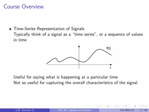
Time-Series Representation of SignalsTypically think of a signal as a “time series”, or a sequence of valuesin time

t

f(t)

Useful for saying what is happening at a particular timeNot so useful for capturing the overall characteristics of the signal.


Idea 1: Frequency Domain Representation of Signals

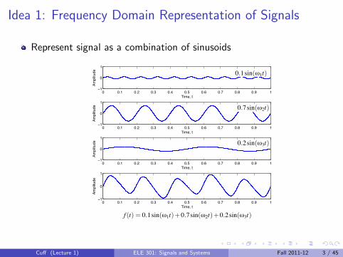
Represent signal as a combination of sinusoids

0 0.1 0.2 0.3 0.4 0.5 0.6 0.7 0.8 0.9 1!1

0

1

Am

plit

ude

Time, t

0 0.1 0.2 0.3 0.4 0.5 0.6 0.7 0.8 0.9 1!1

0

1

Am

plit

ude

Time, t

0 0.1 0.2 0.3 0.4 0.5 0.6 0.7 0.8 0.9 1!1

0

1

Am

plit

ude

Time, t

0 0.1 0.2 0.3 0.4 0.5 0.6 0.7 0.8 0.9 1!1

0

1

Am

plit

ude

Time, t

f (t) = 0.1sin(ω1t)+0.7sin(ω2t)+0.2sin(ω3t)

0.1sin(ω1t)

0.7sin(ω2t)

0.2sin(ω3t)


This example is mostly a sinusoid at frequency ω2, with smallcontributions from sinusoids at frequencies ω1 and ω3.

I Very simple representation (for this case).I Not immediately obvious what the value is at any particular time.

Why use frequency domain representation?I Simpler for many types of signals (AM radio signal, for example)I Many systems are easier to analyze from this perspective (Linear

Systems).I Reveals the fundamental characteristics of a system.

Rapidly becomes an alternate way of thinking about the world.


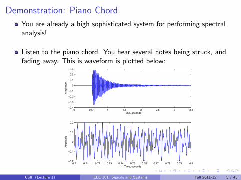
Demonstration: Piano Chord

You are already a high sophisticated system for performing spectralanalysis!

Listen to the piano chord. You hear several notes being struck, andfading away. This is waveform is plotted below:

0 0.5 1 1.5 2 2.5 3 3.5−0.4

−0.3

−0.2

−0.1

0

0.1

0.2

0.3

Time, seconds

Ampl

itude

0.7 0.71 0.72 0.73 0.74 0.75 0.76 0.77 0.78 0.79 0.8−0.2

−0.1

0

0.1

0.2

Time, seconds

Ampl

itude


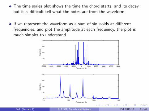
The time series plot shows the time the chord starts, and its decay,but it is difficult tell what the notes are from the waveform.

If we represent the waveform as a sum of sinusoids at differentfrequencies, and plot the amplitude at each frequency, the plot ismuch simpler to understand.

−5000 −4000 −3000 −2000 −1000 0 1000 2000 3000 4000 50000

10

20

30

40

Frequency, Hz

Mag

nitu

de

0 500 1000 15000

10

20

30

40

Mag

nitu

de

Frequency, Hz


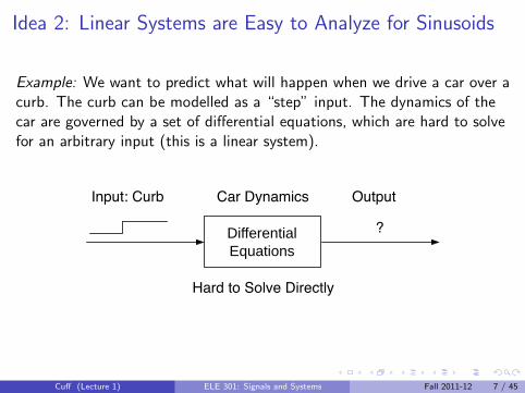
Idea 2: Linear Systems are Easy to Analyze for Sinusoids

Example: We want to predict what will happen when we drive a car over acurb. The curb can be modelled as a “step” input. The dynamics of thecar are governed by a set of differential equations, which are hard to solvefor an arbitrary input (this is a linear system).

Differential Equations

Input: Curb Car Dynamics Output

?

Hard to Solve Directly


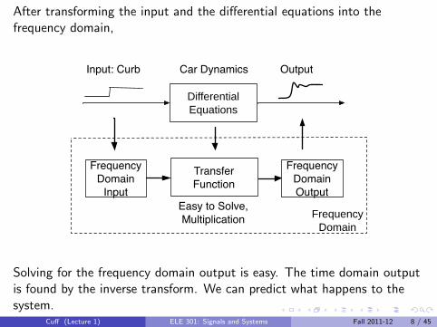
After transforming the input and the differential equations into thefrequency domain,

Frequency Domain

Input

Transfer Function

Frequency Domain Output

Differential Equations

Input: Curb Car Dynamics Output

Easy to Solve,Multiplication Frequency

Domain

Solving for the frequency domain output is easy. The time domain outputis found by the inverse transform. We can predict what happens to thesystem.


Idea 3: Frequency Domain Lets You Control LinearSystems

Often we want a system to do something in particular automaticallyI Airplane to fly levelI Car to go at constant speedI Room to remain at a constant temperature

This is not as trivial as you might think!


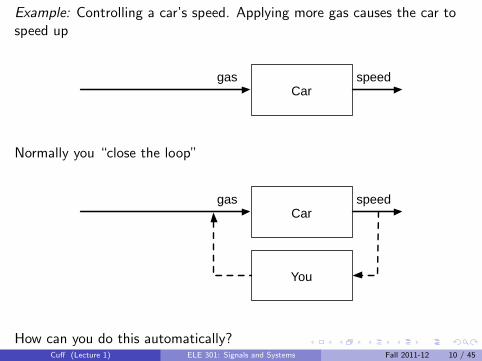
Example: Controlling a car’s speed. Applying more gas causes the car tospeed up

Cargas speed

Normally you “close the loop”

Cargas speed

You

How can you do this automatically?Cuff (Lecture 1) ELE 301: Signals and Systems Fall 2011-12 10 / 45

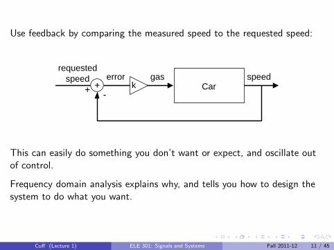
Use feedback by comparing the measured speed to the requested speed:

Cargas speed

requestedspeed ++ -

errork

This can easily do something you don’t want or expect, and oscillate outof control.

Frequency domain analysis explains why, and tells you how to design thesystem to do what you want.


Course Outline

It is useful to represent signals as sums of sinusoids (the frequencydomain)

This is the “correct” domain to analyze linear time-invariant systems

Linear feedback control, sampling, modulation, etc.

What sort of signals and systems are we talking about?


Signals

Typical think of signals in terms of communication and informationI radio signalI broadcast or cable TVI audioI electric voltage or current in a circuit

More generally, any physical or abstract quantity that can bemeasured, or influences one that can be measured, can be thought ofas a signal.

I tension on bike brake cableI roll rate of a spacecraftI concentration of an enzyme in a cellI the price of dollars in eurosI the federal deficit

Very general concept.


Systems

Typical systems take a signal and convert it into another signal,I radio receiverI audio amplifierI modemI microphoneI cell telephoneI cellular metabolismI national and global economies

Internally, a system may contain many different types of signals.

The systems perspective allows you to consider all of these together.

In general, a system transforms input signals into output signals.


Continuous and Discrete Time SignalsMost of the signals we will talk about are functions of time.

There are many ways to classify signals. This class is organizedaccording to whether the signals are continuous in time, or discrete.

A continuous-time signal has values for all points in time in some(possibly infinite) interval.

A discrete time signal has values for only discrete points in time.

t

f(t)

n

f [n]

2 4-2-4 0

Signals can also be a function of space (images) or of space and time(video), and may be continuous or discrete in each dimension.


Types of Systems

Systems are classified according to the types of input and output signals

Continuous-time system has continuous-time inputs and outputs.I AM or FM radioI Conventional (all mechanical) car

Discrete-time system has discrete-time inputs and outputs.I PC computer gameI MatlabI Your mortgage

Hybrid systems are also very important (A/D, D/A converters).I You playing a game on a PCI Modern cars with ECU (electronic control units)I Most commercial and military aircraft


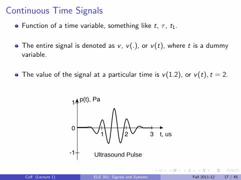
Continuous Time Signals

Function of a time variable, something like t, τ , t1.

The entire signal is denoted as v , v(.), or v(t), where t is a dummyvariable.

The value of the signal at a particular time is v(1.2), or v(t), t = 2.

t, us

p(t), Pa1

-1

01 2 3

Ultrasound Pulse


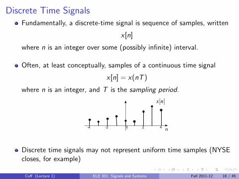
Discrete Time SignalsFundamentally, a discrete-time signal is sequence of samples, written

x [n]

where n is an integer over some (possibly infinite) interval.

Often, at least conceptually, samples of a continuous time signal

x [n] = x(nT )

where n is an integer, and T is the sampling period.

n2 4-2-4 0

x[n]

Discrete time signals may not represent uniform time samples (NYSEcloses, for example)

There may not be an underlying continuous time signal (NYSE closes,again)

There may not be any underlying physical reality (PC computer game)


Summary

A signal is a collection of data

Systems act on signals (inputs and outputs)

Mathematically, they are similar. A signal can be represented by afunction. A system can be represented by a function (the domain isthe space of input signals).

We focus on 1-dimensional signals.

Our systems are not random.


Signal Characteristics and Models

Operations on the time dependence of a signalI Time scalingI Time reversalI Time shiftI Combinations

Signal characteristics

Periodic signals

Complex signals

Signals sizes

Signal Energy and Power


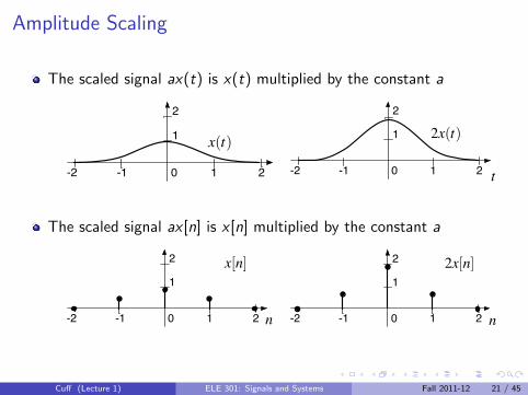
Amplitude Scaling

The scaled signal ax(t) is x(t) multiplied by the constant a

-2 -1 0 1 2

1

2

x(t)

-2 -1 0 1 2

1

2

2x(t)

t

The scaled signal ax [n] is x [n] multiplied by the constant a

-2 -1 0 1 2

1

2 x[n]

n -2 -1 0 1 2

1

2 2x[n]

n


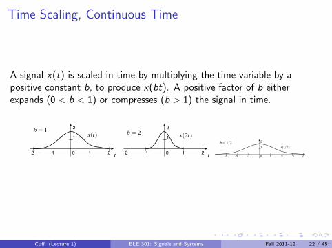
Time Scaling, Continuous Time

A signal x(t) is scaled in time by multiplying the time variable by apositive constant b, to produce x(bt). A positive factor of b eitherexpands (0 < b < 1) or compresses (b > 1) the signal in time.

-2 -1 0 1 2

1

2

t

x(t)b= 1

-2 -1 0 1 2

1

2

t

x(2t)b= 2

-2 -1 0 1 2

1

2

t-3 3

b= 1/2x(t/2)


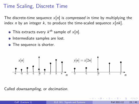
Time Scaling, Discrete Time

The discrete-time sequence x [n] is compressed in time by multiplying theindex n by an integer k , to produce the time-scaled sequence x [nk].

This extracts every kth sample of x [n].

Intermediate samples are lost.

The sequence is shorter.

2 4-2-4 0 1 3-1-3

x[n]

n

y[n] = x[2n]

2-2 0 1-1 n

Called downsampling, or decimation.


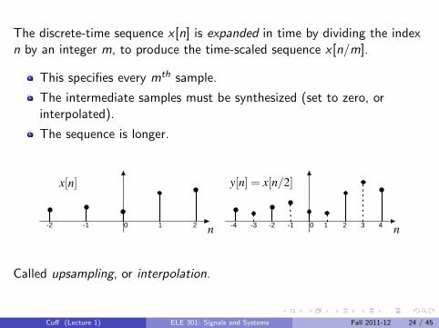
The discrete-time sequence x [n] is expanded in time by dividing the indexn by an integer m, to produce the time-scaled sequence x [n/m].

This specifies every mth sample.

The intermediate samples must be synthesized (set to zero, orinterpolated).

The sequence is longer.

2-2 0 1-1 n

x[n]

2 4-2-4 0 1 3-1-3 n

y[n] = x[n/2]

Called upsampling, or interpolation.


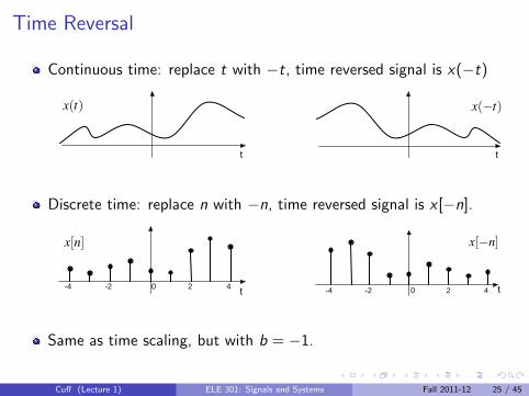
Time Reversal

Continuous time: replace t with −t, time reversed signal is x(−t)

t

x(t)

t

x(−t)

Discrete time: replace n with −n, time reversed signal is x [−n].

t2 4-2-4 0

x[n]

t

x[−n]

2 4-2-4 0

Same as time scaling, but with b = −1.


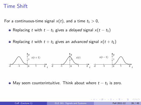
Time Shift

For a continuous-time signal x(t), and a time t1 > 0,

Replacing t with t − t1 gives a delayed signal x(t − t1)

Replacing t with t + t1 gives an advanced signal x(t + t1)

-2 -1 0 1 2

1

2

t

x(t+1)

-2 -1 0 1 2

1

2

t

x(t)

-2 -1 0 1 2

1

2

t

x(t−1)

May seem counterintuitive. Think about where t − t1 is zero.


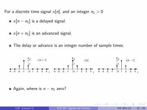
For a discrete time signal x [n], and an integer n1 > 0

x [n − n1] is a delayed signal.

x [n + n1] is an advanced signal.

The delay or advance is an integer number of sample times.

-2 -1 0 1 2

1

2

t-4 -3 3 4

x[n+1]

-2 -1 0 1 2

1

2

t-4 -3 3 4

x[n]

-2 -1 0 1 2

1

2

t-4 -3 3 4

x[n−1]

Again, where is n − n1 zero?


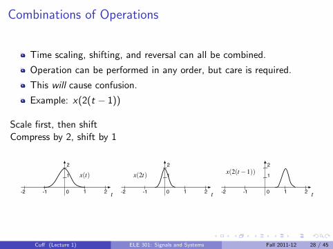
Combinations of Operations

Time scaling, shifting, and reversal can all be combined.

Operation can be performed in any order, but care is required.

This will cause confusion.

Example: x(2(t − 1))

Scale first, then shiftCompress by 2, shift by 1

-2 -1 0 1 2

1

2

t

x(t)

-2 -1 0 1 2

1

2

t

x(2t)

-2 -1 0 1 2

1

2

t

x(2(t−1))


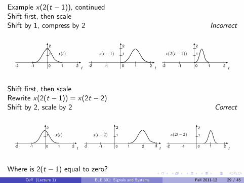
Example x(2(t − 1)), continuedShift first, then scaleShift by 1, compress by 2 Incorrect

-2 -1 0 1 2

1

2

t

x(t)

-2 -1 0 1 2

1

2

t

x(t−1)

-2 -1 0 1 2

1

2

t

x(2(t−1))

Shift first, then scaleRewrite x(2(t − 1)) = x(2t − 2)Shift by 2, scale by 2 Correct

-2 -1 0 1 2

1

2

t

x(t)

-2 -1 0 1 2

1

2

t3

x(t−2)

-2 -1 0 1 2

1

2

t

x(2t−2)

Where is 2(t − 1) equal to zero?


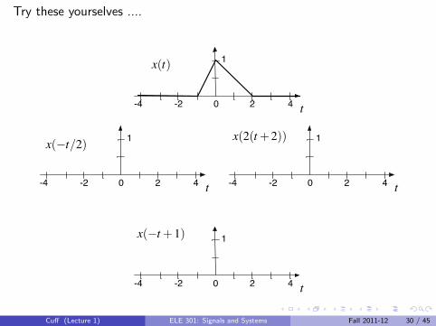
Try these yourselves ....

t-4 -2 0 2 4

1x(t)

-4 -2 0 2 4

1

t

x(−t/2)

-4 -2 0 2 4

1

t

x(2(t+2))

-4 -2 0 2 4

1

t

x(−t+1)


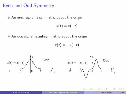
Even and Odd Symmetry

An even signal is symmetric about the origin

x(t) = x(−t)

An odd signal is antisymmetric about the origin

x(t) = −x(−t)

-2 -1 0 1 2

1

2

t

Evenx(t) = x(−t)

-2 -1 0 1 2

1

2

t

Oddx(t) =−x(−t)


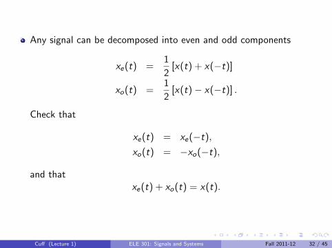
Any signal can be decomposed into even and odd components

xe(t) =1

2[x(t) + x(−t)]

xo(t) =1

2[x(t)− x(−t)] .

Check that

xe(t) = xe(−t),

xo(t) = −xo(−t),

and thatxe(t) + xo(t) = x(t).


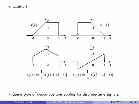
Example

-1 0 1

1

2

t -1 0 1

1

2

t

-1 0 1

1

2

t -1 0 1

1

2

t

x(t) x(−t)

xe(t) =12 [x(t)+ x(−t)] xo(t) =

12 [x(t)− x(−t)]

Same type of decomposition applies for discrete-time signals.


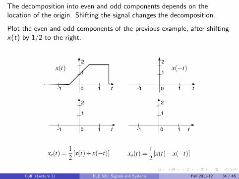
The decomposition into even and odd components depends on thelocation of the origin. Shifting the signal changes the decomposition.

Plot the even and odd components of the previous example, after shiftingx(t) by 1/2 to the right.

-1 0 1

1

2

t -1 0 1

1

2

t

-1 0 1

1

2

t -1 0 1

1

2

t

x(t) x(−t)

xe(t) =12 [x(t)+ x(−t)] xo(t) =

12 [x(t)− x(−t)]


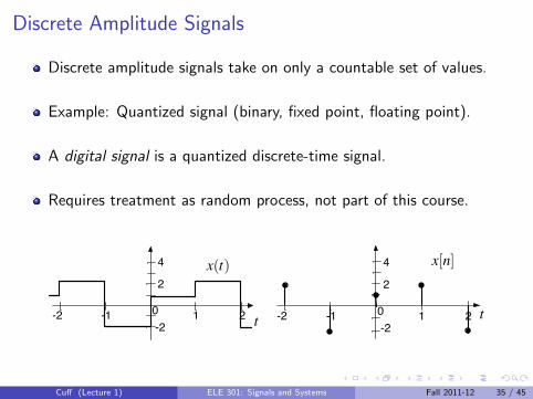
Discrete Amplitude Signals

Discrete amplitude signals take on only a countable set of values.

Example: Quantized signal (binary, fixed point, floating point).

A digital signal is a quantized discrete-time signal.

Requires treatment as random process, not part of this course.

-2 -1 0 1 2

2

4

t

x(t)

-2-2 -1 0 1 2

2

4

t-2

x[n]


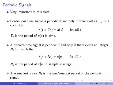
Periodic Signals

Very important in this class.

Continuous time signal is periodic if and only if there exists a T0 > 0such that

x(t + T0) = x(t) for all t

T0 is the period of x(t) in time.

A discrete-time signal is periodic if and only if there exists an integerN0 > 0 such that

x [n + N0] = x [n] for all n

N0 is the period of x [n] in sample spacings.

The smallest T0 or N0 is the fundamental period of the periodicsignal.


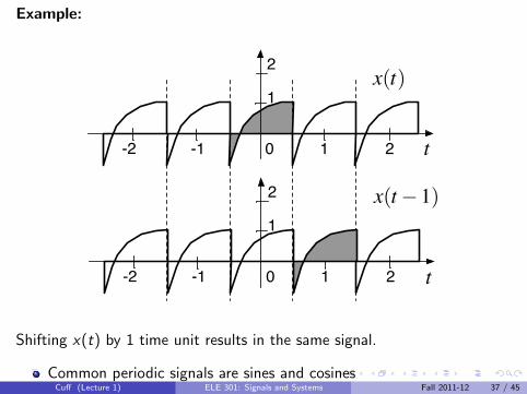
Example:

-2 -1 0 1 2

1

2

t

x(t)

-2 -1 0 1 2

1

2

t

x(t−1)

Shifting x(t) by 1 time unit results in the same signal.

Common periodic signals are sines and cosines

x(t) = A cos(2πt/T0 − θ)

x [n] = A cos(2πn/N0 − θ)

An aperiodic signal is a signal that is not periodic.

Seems like a simple concept, but there are some interesting casesI Is

x [n] = A cos(2πna− θ)

periodic for any a?I Is the sum of periodic discrete-time signals periodic?I Is the sum of periodic continuous-time signals periodic?


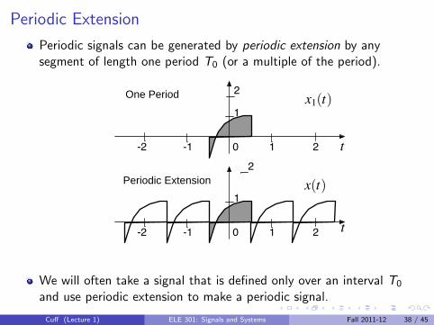
Periodic Extension

Periodic signals can be generated by periodic extension by anysegment of length one period T0 (or a multiple of the period).

-2 -1 0 1 2

1

2

t

-2 -1 0 1 2

1

2

t

x(t)

x1(t)One Period

Periodic Extension

We will often take a signal that is defined only over an interval T0

and use periodic extension to make a periodic signal.


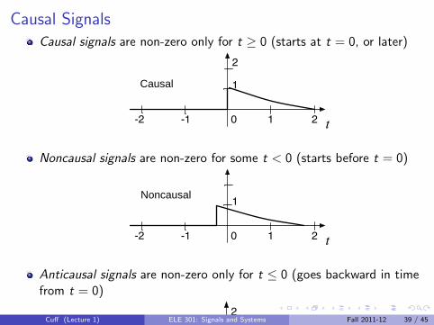
Causal SignalsCausal signals are non-zero only for t ≥ 0 (starts at t = 0, or later)

-2 -1 0 1 2

1

2

t

Causal

Noncausal signals are non-zero for some t < 0 (starts before t = 0)

-2 -1 0 1 2

1

t

Noncausal

Anticausal signals are non-zero only for t ≤ 0 (goes backward in timefrom t = 0)

-2 -1 0 1 2

1

2

t

AnticausalCuff (Lecture 1) ELE 301: Signals and Systems Fall 2011-12 39 / 45

Complex Signals

So far, we have only considered real (or integer) valued signals.

Signals can also be complex

z(t) = x(t) + jy(t)

where x(t) and y(t) are each real valued signals, and j =√−1.

Arises naturally in many problemsI Convenient representation for sinusoidsI CommunicationsI Radar, sonar, ultrasound


Review of Complex Numbers

Complex number in Cartesian form: z = x + jy

x = <z , the real part of z

y = =z , the imaginary part of z

x and y are also often called the in-phase and quadrature componentsof z .

j =√−1 (engineering notation)

i =√−1 (physics, chemistry, mathematics)


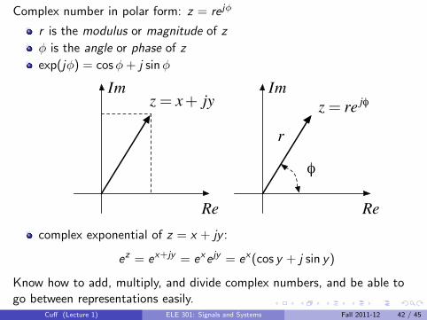
Complex number in polar form: z = re jφ

r is the modulus or magnitude of z

φ is the angle or phase of z

exp(jφ) = cosφ+ j sinφ

Im

Re

z= x+ jy

r

φ

Im

Re

z= re jφ

complex exponential of z = x + jy :

ez = ex+jy = exe jy = ex(cos y + j sin y)

Know how to add, multiply, and divide complex numbers, and be able togo between representations easily.


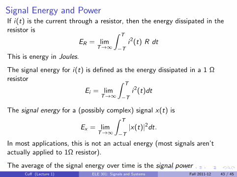
Signal Energy and PowerIf i(t) is the current through a resistor, then the energy dissipated in theresistor is

ER = limT→∞

∫ T

−Ti2(t) R dt

This is energy in Joules.

The signal energy for i(t) is defined as the energy dissipated in a 1 Ωresistor

Ei = limT→∞

∫ T

−Ti2(t)dt

The signal energy for a (possibly complex) signal x(t) is

Ex = limT→∞

∫ T

−T|x(t)|2dt.

In most applications, this is not an actual energy (most signals aren’tactually applied to 1Ω resistor).

The average of the signal energy over time is the signal power

Px = limT→∞

1

2T

∫ T

−T|x(t)|2dt.

Again, in most applications this is not an actual power.

Signals are classified by whether they have finite energy or power,

An energy signal x(t) has energy 0 < Ex <∞

A power signal x(t) has power 0 < Px <∞

These two types of signals will require much different treatment later.


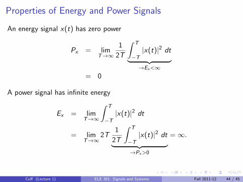
Properties of Energy and Power Signals

An energy signal x(t) has zero power

Px = limT→∞

1

2T

∫ T

−T|x(t)|2 dt︸︷︷︸→Ex<∞

= 0

A power signal has infinite energy

Ex = limT→∞

∫ T

−T|x(t)|2 dt

= limT→∞

2T1

2T

∫ T

−T|x(t)|2 dt︸︷︷︸

→Px>0

=∞.


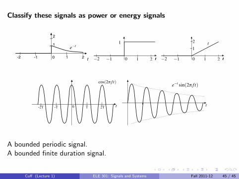
Classify these signals as power or energy signals

-2 -1 0 1 2

1

2

t

e−t1

tt1 2−1 0−2

1

tt1 2−1 0−2

2 t

T 2T-2T -T 0

cos(2π f t)

t t

e−t sin(2π f t)

A bounded periodic signal.A bounded finite duration signal.


lecture 1 ele 301: signals and systems - princeton.educuff/ele301/files/lecture1_1.pdf · ele 301:...

Documents