lecture 1 linear quadratic regulator: discrete-time ﬁnite ... · ee363 winter 2008-09 lecture 1...

EE363 Winter 2008-09

Lecture 1

Linear quadratic regulator:Discrete-time finite horizon

• LQR cost function

• multi-objective interpretation

• LQR via least-squares

• dynamic programming solution

• steady-state LQR control

• extensions: time-varying systems, tracking problems

1–1

LQR problem: background

discrete-time system xt+1 = Axt + But, x0 = xinit

problem: choose u0, u1, . . . so that

• x0, x1, . . . is ‘small’, i.e., we get good regulation or control

• u0, u1, . . . is ‘small’, i.e., using small input effort or actuator authority

• we’ll define ‘small’ soon

• these are usually competing objectives, e.g., a large u can drive x tozero fast

linear quadratic regulator (LQR) theory addresses this question

Linear quadratic regulator: Discrete-time finite horizon 1–2

LQR cost function

we define quadratic cost function

J(U) =N−1∑

τ=0

(xT

τ Qxτ + uTτ Ruτ

)+ xT

NQfxN

where U = (u0, . . . , uN−1) and

Q = QT ≥ 0, Qf = QTf ≥ 0, R = RT > 0

are given state cost, final state cost, and input cost matrices


• N is called time horizon (we’ll consider N = ∞ later)

• first term measures state deviation

• second term measures input size or actuator authority

• last term measures final state deviation

• Q, R set relative weights of state deviation and input usage

• R > 0 means any (nonzero) input adds to cost J

LQR problem: find ulqr0 , . . . , u

lqrN−1 that minimizes J(U)


Comparison to least-norm input

c.f. least-norm input that steers x to xN = 0:

• no cost attached to x0, . . . , xN−1

• xN must be exactly zero

we can approximate the least-norm input by taking

R = I, Q = 0, Qf large, e.g., Qf = 108I


Multi-objective interpretation

common form for Q and R:

R = ρI, Q = Qf = CTC

where C ∈ Rp×n and ρ ∈ R, ρ > 0

cost is then

J(U) =N∑

τ=0

‖yτ‖2 + ρ

N−1∑

τ=0

‖uτ‖2

where y = Cx

here√

ρ gives relative weighting of output norm and input norm


Input and output objectives

fix x0 = xinit and horizon N ; for any input U = (u0, . . . , uN−1) define

• input cost Jin(U) =∑N−1

τ=0 ‖uτ‖2

• output cost Jout(U) =∑N

τ=0 ‖yτ‖2

these are (competing) objectives; we want both small

LQR quadratic cost is Jout + ρJin


plot (Jin, Jout) for all possible U :

Jin

Jout U1

U2

U3

• shaded area shows (Jin, Jout) achieved by some U

• clear area shows (Jin, Jout) not achieved by any U


three sample inputs U1, U2, and U3 are shown

• U3 is worse than U2 on both counts (Jin and Jout)

• U1 is better than U2 in Jin, but worse in Jout

interpretation of LQR quadratic cost:

J = Jout + ρJin = constant

corresponds to a line with slope −ρ on (Jin, Jout) plot


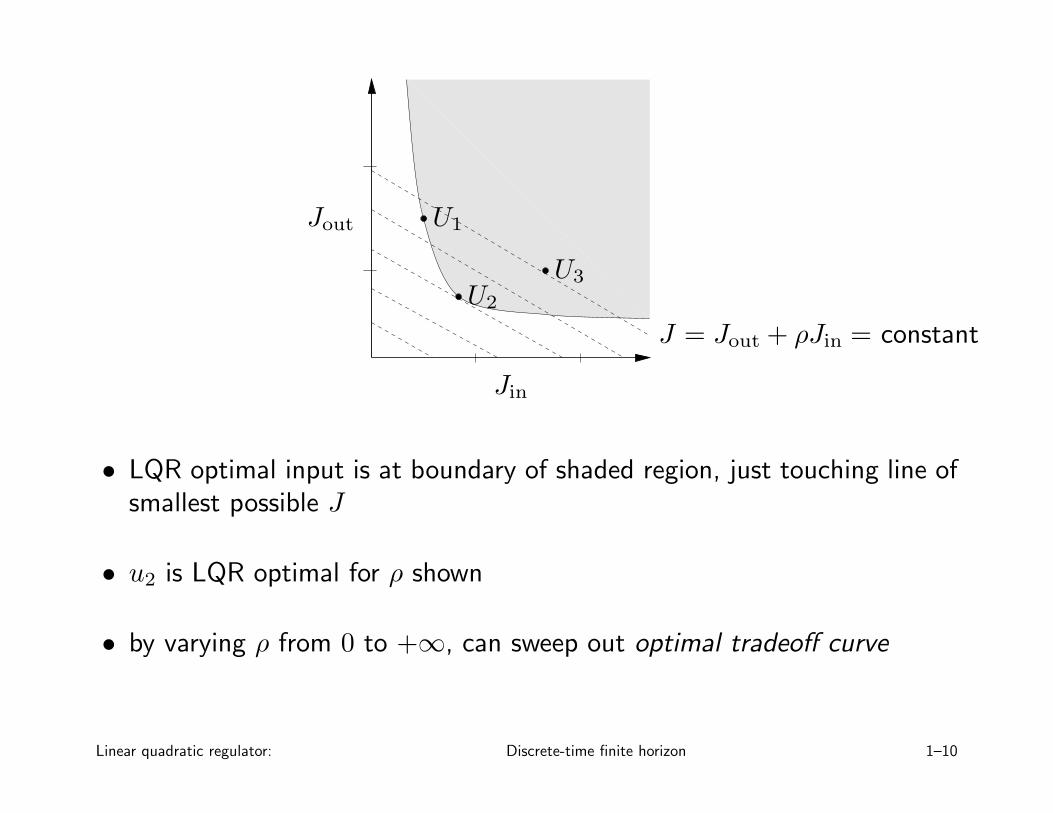
Jin

Jout U1

U2

U3

J = Jout + ρJin = constant

• LQR optimal input is at boundary of shaded region, just touching line ofsmallest possible J

• u2 is LQR optimal for ρ shown

• by varying ρ from 0 to +∞, can sweep out optimal tradeoff curve


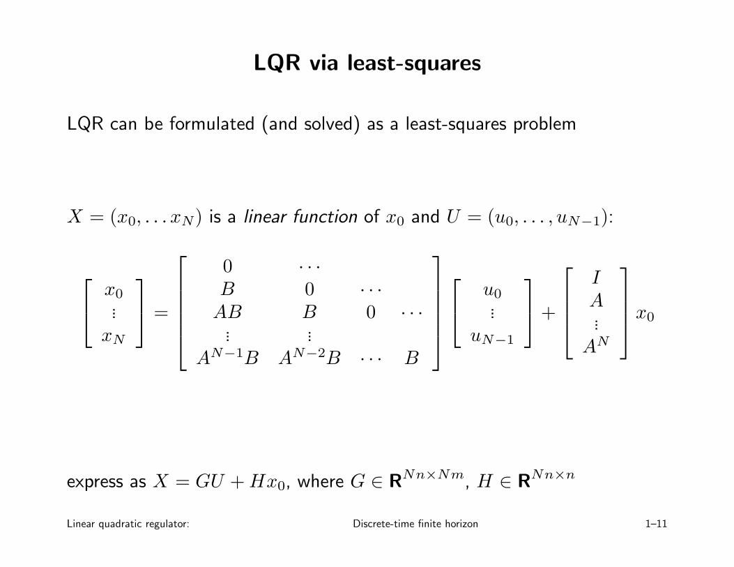
LQR via least-squares

LQR can be formulated (and solved) as a least-squares problem

X = (x0, . . . xN) is a linear function of x0 and U = (u0, . . . , uN−1):

x0...

xN

=

0 · · ·B 0 · · ·

AB B 0 · · ·... ...

AN−1B AN−2B · · · B

u0...

uN−1

+

I

A...

AN

x0

express as X = GU + Hx0, where G ∈ RNn×Nm, H ∈ RNn×n


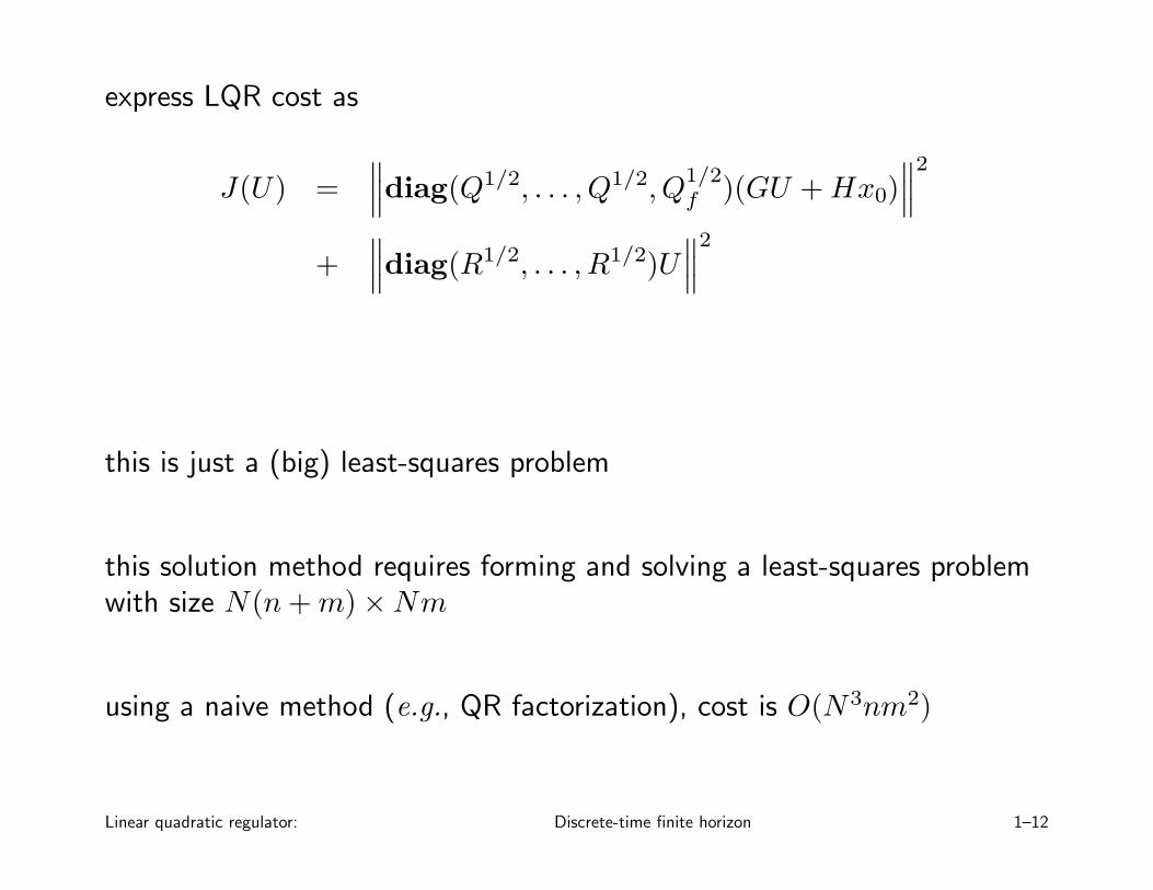
express LQR cost as

J(U) =∥∥∥diag(Q1/2, . . . , Q1/2, Q

1/2f )(GU + Hx0)

∥∥∥

2

+∥∥∥diag(R1/2, . . . , R1/2)U

∥∥∥

2

this is just a (big) least-squares problem

this solution method requires forming and solving a least-squares problemwith size N(n + m) × Nm

using a naive method (e.g., QR factorization), cost is O(N3nm2)


Dynamic programming solution

• gives an efficient, recursive method to solve LQR least-squares problem;cost is O(Nn3)

• (but in fact, a less naive approach to solve the LQR least-squaresproblem will have the same complexity)

• useful and important idea on its own

• same ideas can be used for many other problems


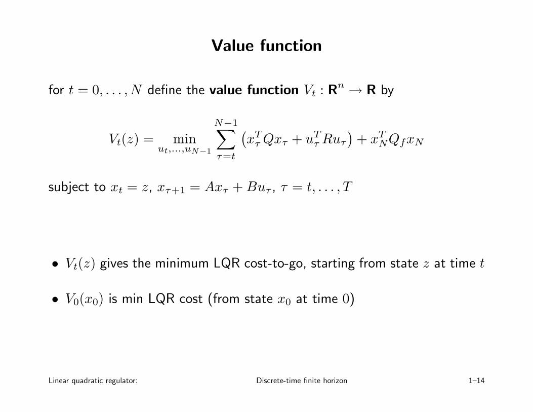
Value function

for t = 0, . . . , N define the value function Vt : Rn → R by

Vt(z) = minut,...,uN−1

N−1∑

τ=t

(xT

τ Qxτ + uTτ Ruτ

)+ xT

NQfxN

subject to xt = z, xτ+1 = Axτ + Buτ , τ = t, . . . , T

• Vt(z) gives the minimum LQR cost-to-go, starting from state z at time t

• V0(x0) is min LQR cost (from state x0 at time 0)


we will find that

• Vt is quadratic, i.e., Vt(z) = zTPtz, where Pt = PTt ≥ 0

• Pt can be found recursively, working backward from t = N

• the LQR optimal u is easily expressed in terms of Pt

cost-to-go with no time left is just final state cost:

VN(z) = zTQfz

thus we have PN = Qf


Dynamic programming principle

• now suppose we know Vt+1(z)

• what is the optimal choice for ut?

• choice of ut affects

– current cost incurred (through uTt Rut)

– where we land, xt+1 (hence, the min-cost-to-go from xt+1)

• dynamic programming (DP) principle:

Vt(z) = minw

(zTQz + wTRw + Vt+1(Az + Bw)

)

– zTQz + wTRw is cost incurred at time t if ut = w

– Vt+1(Az + Bw) is min cost-to-go from where you land at t + 1


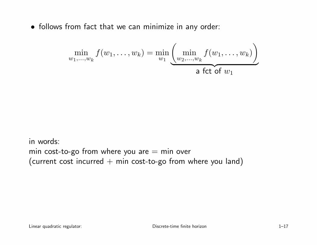
• follows from fact that we can minimize in any order:

minw1,...,wk

f(w1, . . . , wk) = minw1

(

minw2,...,wk

f(w1, . . . , wk)

)

︸︷︷︸

a fct of w1

in words:min cost-to-go from where you are = min over(current cost incurred + min cost-to-go from where you land)


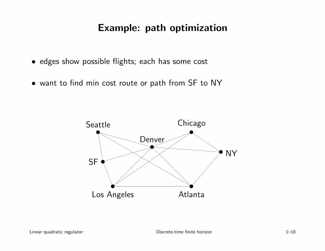
Example: path optimization

• edges show possible flights; each has some cost

• want to find min cost route or path from SF to NY

SFNY

Seattle

Atlanta

Chicago

Denver

Los Angeles


dynamic programming (DP):

• V (i) is min cost from airport i to NY, over all possible paths

• to find min cost from city i to NY: minimize sum of flight cost plus mincost to NY from where you land, over all flights out of city i

(gives optimal flight out of city i on way to NY)

• if we can find V (i) for each i, we can find min cost path from any cityto NY

• DP principle: V (i) = minj(cji + V (j)), where cji is cost of flight fromi to j, and minimum is over all possible flights out of i


HJ equation for LQR

Vt(z) = zTQz + minw

(wTRw + Vt+1(Az + Bw)

)

• called DP, Bellman, or Hamilton-Jacobi equation

• gives Vt recursively, in terms of Vt+1

• any minimizing w gives optimal ut:

ulqrt = argmin

w

(wTRw + Vt+1(Az + Bw)

)


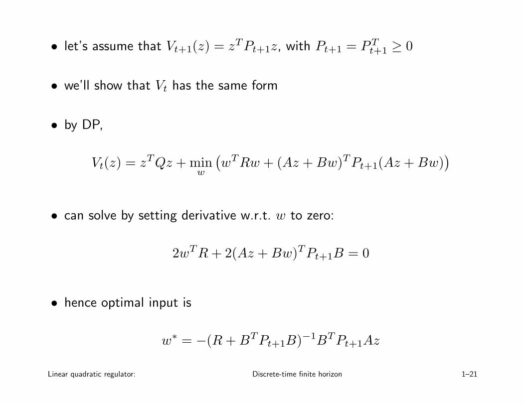
• let’s assume that Vt+1(z) = zTPt+1z, with Pt+1 = PTt+1 ≥ 0

• we’ll show that Vt has the same form

• by DP,

Vt(z) = zTQz + minw

(wTRw + (Az + Bw)TPt+1(Az + Bw)

)

• can solve by setting derivative w.r.t. w to zero:

2wTR + 2(Az + Bw)TPt+1B = 0

• hence optimal input is

w∗ = −(R + BTPt+1B)−1BTPt+1Az


• and so (after some ugly algebra)

Vt(z) = zTQz + w∗TRw∗ + (Az + Bw∗)TPt+1(Az + Bw∗)

= zT(Q + ATPt+1A − ATPt+1B(R + BTPt+1B)−1BTPt+1A

)z

= zTPtz

where

Pt = Q + ATPt+1A − ATPt+1B(R + BTPt+1B)−1BTPt+1A

• easy to show Pt = PTt ≥ 0


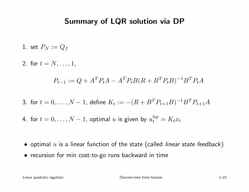
Summary of LQR solution via DP

1. set PN := Qf

2. for t = N, . . . , 1,

Pt−1 := Q + ATPtA − ATPtB(R + BTPtB)−1BTPtA

3. for t = 0, . . . , N − 1, define Kt := −(R + BTPt+1B)−1BTPt+1A

4. for t = 0, . . . , N − 1, optimal u is given by ulqrt = Ktxt

• optimal u is a linear function of the state (called linear state feedback)

• recursion for min cost-to-go runs backward in time


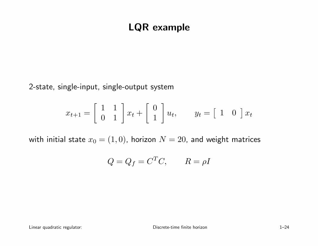
LQR example

2-state, single-input, single-output system

xt+1 =

[1 10 1

]

xt +

[01

]

ut, yt =[

1 0]xt

with initial state x0 = (1, 0), horizon N = 20, and weight matrices

Q = Qf = CTC, R = ρI


optimal trade-off curve of Jin vs. Jout:

0 0.1 0.2 0.3 0.4 0.5 0.6 0.7 0.8 0.9 10

1

2

3

4

5

6

Jin

Jout

circles show LQR solutions with ρ = 0.3, ρ = 10


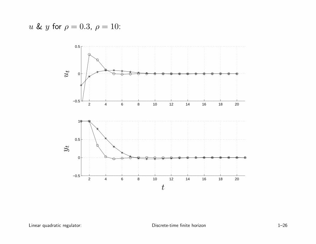
u & y for ρ = 0.3, ρ = 10:

2 4 6 8 10 12 14 16 18 20−0.5

0

0.5

2 4 6 8 10 12 14 16 18 20−0.5

0

0.5

1

t

ut

yt


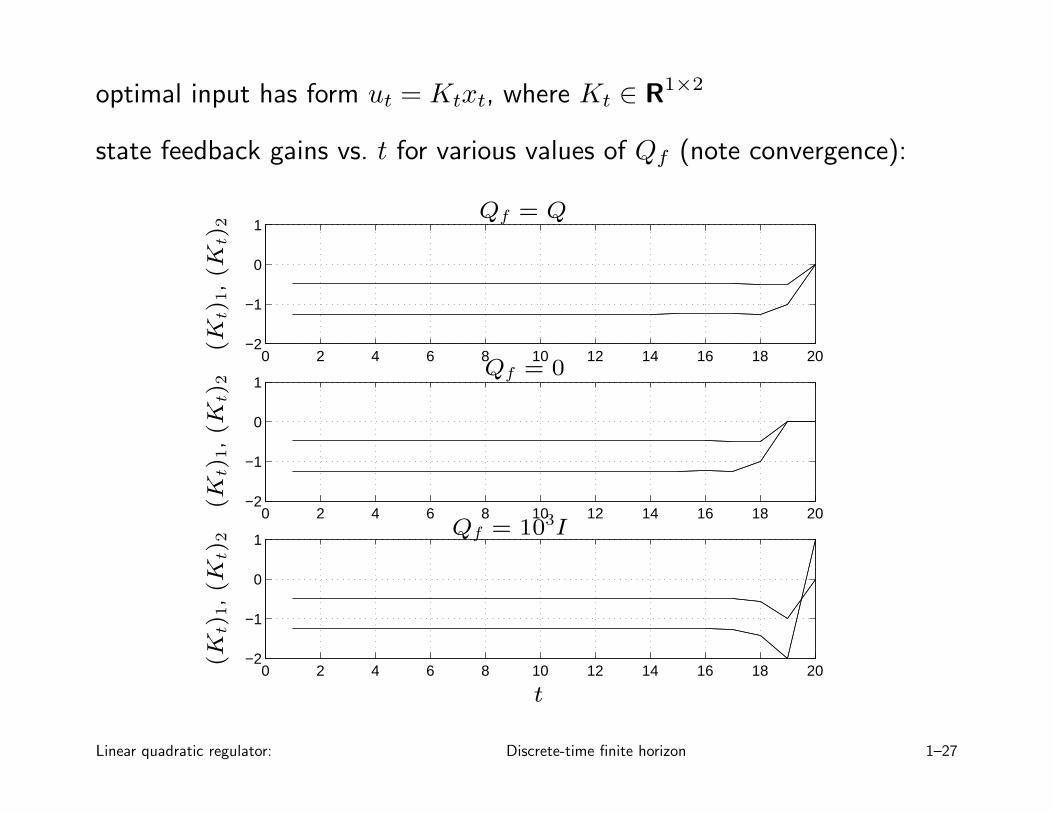
optimal input has form ut = Ktxt, where Kt ∈ R1×2

state feedback gains vs. t for various values of Qf (note convergence):

0 2 4 6 8 10 12 14 16 18 20−2

−1

0

1

0 2 4 6 8 10 12 14 16 18 20−2

−1

0

1

0 2 4 6 8 10 12 14 16 18 20−2

−1

0

1

t

(Kt)

1,(K

t)2

(Kt)

1,(K

t)2

(Kt)

1,(K

t)2

Qf = Q

Qf = 0

Qf = 103I


Steady-state regulator

usually Pt rapidly converges as t decreases below N

limit or steady-state value Pss satisfies

Pss = Q + ATPssA − ATPssB(R + BTPssB)−1BTPssA

which is called the (DT) algebraic Riccati equation (ARE)

• Pss can be found by iterating the Riccati recursion, or by direct methods

• for t not close to horizon N , LQR optimal input is approximately alinear, constant state feedback

ut = Kssxt, Kss = −(R + BTPssB)−1BTPssA

(very widely used in practice; more on this later)


Time-varying systems

LQR is readily extended to handle time-varying systems

xt+1 = Atxt + Btut

and time-varying cost matrices

J =N−1∑

τ=0

(xT

τ Qτxτ + uTτ Rτuτ

)+ xT

NQfxN

(so Qf is really just QN)

DP solution is readily extended, but (of course) there need not be asteady-state solution


Tracking problems

we consider LQR cost with state and input offsets:

J =N−1∑

τ=0

(xτ − xτ)TQ(xτ − xτ)

+

N−1∑

τ=0

(uτ − uτ)TR(uτ − uτ)

(we drop the final state term for simplicity)

here, xτ and uτ are given desired state and input trajectories

DP solution is readily extended, even to time-varying tracking problems


Gauss-Newton LQR

nonlinear dynamical system: xt+1 = f(xt, ut), x0 = xinit

objective is

J(U) =

N−1∑

τ=0

(xT

τ Qxτ + uTτ Ruτ

)+ xT

NQfxN

where Q = QT ≥ 0, Qf = QTf ≥ 0, R = RT > 0

start with a guess for U , and alternate between:

• linearize around current trajectory

• solve associated LQR (tracking) problem

sometimes converges, sometimes to the globally optimal U


some more detail:

• let u denote current iterate or guess

• simulate system to find x, using xt+1 = f(xt, ut)

• linearize around this trajectory: δxt+1 = Atδxt + Btδut

At = Dxf(xt, ut) Bt = Duf(xt, ut)

• solve time-varying LQR tracking problem with cost

J =

N−1∑

τ=0

(xτ + δxτ)TQ(xτ + δxτ)

+N−1∑

τ=0

(uτ + δuτ)TR(uτ + δuτ)

• for next iteration, set ut := ut + δut


lecture 1 linear quadratic regulator: discrete-time ﬁnite ... · ee363 winter 2008-09 lecture 1...

Documents