lecture 1 the new keynesian model of monetary …lecture 2 - policy analysis in the new keynesian...
TRANSCRIPT

Lecture 1
The New Keynesian Model of Monetary Policy
Lecturer – Campbell Leith
University of Glasgow
The New Keynesian model of monetary policy is
becoming increasingly standard in the analysis of
monetary policy. This particular treatment follows Carl
Walsh (2003), “Monetary Theory and Policy”, chapter 5.
Another good reference is by Richard Clarida, Jordi Galí,
and Mark Gertler, “The Science of Monetary Policy: A New
Keynesian Perspective”, Journal of Economic Literature Vol.
XXXVII (December 1999), pp. 1661–1707
Key Features:
• Households consume a basket of goods and supply
labour to imperfectly competitive firms.
• Firms only change prices after a random interval of
time (i.e. prices are sticky).
• Since prices are sticky monetary policy can have
real effects in the short-run.
Problems we need to analyse:
• Households’ Problems: (1)allocation of spending
across goods, and (2)allocation of spending across
time.
• Firms Pricing/Production decision.
Households:
The utility function of the representative household is
given by,
11 1
0 1 1 1
bi t i t i t i
ti t i
C M NEb P
σ ηγβ χσ η
−− +∞+ + +
= +
⎡ ⎤⎛ ⎞⎢ ⎥+ −⎜ ⎟− − +⎢ ⎥⎝ ⎠⎣ ⎦
∑ (1)
Where Ct+i is a basket of goods, M/P are real money
balances and N is labour supply.
The consumption basket is defined in the following CES
form,
1 1 1
0t jtC c dj
θθ θθ− −⎡ ⎤
= ⎢ ⎥⎣ ⎦∫ (2)
where θ is the elasticity of demand for the individual
goods and 1θ > .
Problem 1 - The optimal allocation of a given
consumption expenditure across the individual goods in
the consumption basket.

This initial problem amounts to minimizing the cost of
buying Ct,
1
0
minjt jt
jtp c dj
c ∫ (3)
subject to, 1 1 1
0t jtC c dj
θθ θθ− −⎡ ⎤
= ⎢ ⎥⎣ ⎦∫ (4)
Form the Lagrangian,
1 1 1 1
0 0t jt jt t t jtL p c dj C c dj
θθ θθψ− −
⎛ ⎞⎡ ⎤⎜ ⎟= + − ⎢ ⎥⎜ ⎟⎣ ⎦⎜ ⎟
⎝ ⎠∫ ∫ (5)
The first order condition with respect to good j is,
11 1 11
0
0tjt t jt jt
jt
L p c dj cc
θ θθ θψ− − −
⎛ ⎞⎡ ⎤∂ ⎜ ⎟= − =⎢ ⎥⎜ ⎟∂ ⎣ ⎦⎜ ⎟
⎝ ⎠∫ (6)
Using the definition of the consumption basket,
1
0jt t t jtp C cθ θψ−
− = (7)
Rearranging,
jt
jt tt
pc C
θ
ψ
−⎛ ⎞
= ⎜ ⎟⎝ ⎠ (8)

From the definition of the composite level of
consumption this implies,
1 11 1 1
1
0 0
1jtt t jt t
t t
pC C dj p dj C
θθ θ θ
θ θθ θθ
ψ ψ
− −− −
−−
⎡ ⎤⎡ ⎤ ⎡ ⎤⎛ ⎞ ⎛ ⎞⎢ ⎥⎢ ⎥= = ⎢ ⎥⎜ ⎟ ⎜ ⎟⎢ ⎥⎢ ⎥⎝ ⎠ ⎝ ⎠ ⎣ ⎦⎢ ⎥⎣ ⎦
⎣ ⎦
∫ ∫ (9)
Solving for the lagrange multiplier,
11 1
1
0t jt tp dj P
θθψ
−−⎡ ⎤
= ≡⎢ ⎥⎣ ⎦∫ (10)
The lagrange multiplier can be considered to be the price
index appropriate for the consumption bundle.
Substituting this back into the first order condition, (8)
yields,
jt
jt tt
pc C
P
θ−⎛ ⎞
= ⎜ ⎟⎝ ⎠ (11)
As θ → ∞ we move towards perfect competition and firms
enjoy less market power. This equation is effectively the
demand curve facing the firm j for its product.

Problem 2 - The Household’s Intertemporal Problem:
Before maximizing utility we need to consider the
households budget constraint. This is given, in nominal
terms by,
1 1 1(1 )t t t t t t t t t tPC M B W N M R B− − −+ + = + + + + ∏ (12)
Where tΠ are the profits from the imperfectly
competitive firms redistributed to households.
Dividing by the price level P, we can rewrite this in real
terms as,
1 11(1 )t t t t t t
t t tt t t t t t
M B W M BC N RP P P P P P
− −−
∏+ + = + + + + (13)
Therefore, forming the Lagrangian for the problem,
11 1
01 1
1
1 1 1
(1 )
bi t i t i t i
t it
it i t i t i t i t i t i
t i t i t i t it i t i t i t i t i t i
C M Nb P
EM B W M BC N RP P P P P P
σ ηγβ χσ η
λ
−− ++ + +
∞+
=+ + + + − + − +
+ + + + −+ + + + + +
⎛ ⎞⎡ ⎤⎛ ⎞⎜ ⎟⎢ ⎥+ −⎜ ⎟− − +⎜ ⎟⎢ ⎥⎝ ⎠⎣ ⎦⎜ ⎟⎜ ⎟⎛ ⎞∏
+ + + − − − + −⎜ ⎟⎜ ⎟⎜ ⎟⎝ ⎠⎝ ⎠
∑
(14)

The first order conditions for consumption are given by,
( ) 0it i t iC σβ λ−+ ++ = (15)
Money,
11 1
0b
t i t it i t i
t t i
M PP P
γβ λ λ−
+ ++ + +
+ + +
⎛ ⎞+ − =⎜ ⎟
⎝ ⎠ (16)
Labour Supply,
0i t it i t i
t i
WNP
ηβ χ λ ++ +
+
− − = (17)
Bonds,
11
(1 ) 0t it i t i t i
t i
PRP
λ λ ++ + + +
+ +
− + = (18)
Using the equation of motion for the Lagrange multiplier
we can obtain the Euler equation for consumption,
11
(1 ) tt t t t
t
PC R E CP
σ σβ− −+
+
⎛ ⎞= + ⎜ ⎟
⎝ ⎠ (19)
Money,
1
b
t tt
t t
M RCP R
σγ−
−⎛ ⎞=⎜ ⎟ +⎝ ⎠
(20)
Labour Supply,
t
t tt
WN CP
η σχ −= (21)

Firms:
Firms are profit maximisers, but they face three
constraints. Firstly they must work with a given
production technology given by,
jt t jtc Z N= (22)
which is linear in labour input (there is no capital) and an
aggregate productivity disturbance Z. The expected value
of Z is 1.
Secondly, the face the downward sloping demand curve
given by,
jt
jt tt
pc C
P
θ−⎛ ⎞
= ⎜ ⎟⎝ ⎠ (23)
Finally, we are going to adopt nominal inertia in the form
of Calvo (1983) contracts. In any period (1 )ω− of firms
are randomly chosen to be able to change their price.
Therefore in setting prices, firms must take account of
future economic conditions since the price they set today
may still be in place tomorrow.
Since labour is the only input in the productive process
the real marginal cost of production is given by,
/t t
tt
W PMCZ
= (24)
The firm’s pricing problem then becomes,
1
,0
jt jtit i t i t i t i
i t i t i
p pE MC C
P P
θ θ
ω− −
∞
+ + += + +
⎡ ⎤⎛ ⎞ ⎛ ⎞⎢ ⎥∆ −⎜ ⎟ ⎜ ⎟⎢ ⎥⎝ ⎠ ⎝ ⎠⎣ ⎦
∑ (25)
This problem is the same for all firms able to change
their prices in period t.
The first order condition for the optimal price, p*
is given by,
* *
, *0
1(1 ) 0i t tt i t i t i t i
i t i t t i
p pE MC CP p P
θ θ
ω θ θ− −
∞
+ + += + +
⎡ ⎤⎛ ⎞ ⎛ ⎞⎛ ⎞⎢ ⎥∆ − − =⎜ ⎟ ⎜ ⎟⎜ ⎟⎢ ⎥⎝ ⎠ ⎝ ⎠⎝ ⎠⎣ ⎦
∑
(26)
Flexible Price Equilibrium:
It is helpful to examine the equilibrium when prices are
flexible.
When firms are able to adjust their prices every period
then this reduces to, *
1t
tt
p MCP
θθ
⎛ ⎞ ⎛ ⎞=⎜ ⎟ ⎜ ⎟−⎝ ⎠⎝ ⎠ (27)
Where 1θ
θ⎛ ⎞⎜ ⎟−⎝ ⎠ reflects the markup of prices over
marginal costs due to the fact that firms enjoy market
power.
Since, when prices are flexible, all firms will be setting
the same price there are no relative price differences and
using the definition of marginal cost this can be written
as,
/1
1t t
t
W PZ
θθ
⎛ ⎞= ⎜ ⎟−⎝ ⎠ (28)

Using the labour supply condition on the part of the
household we obtain,
/( 1)t t t
t t
W Z NP C
η
σ
χθ θ −= =
− (29)
We now need to consider how to log-linearise. Take
natural logarithms of both sides of equation (29) to
obtain,
ln ln/( 1)
t t
t
Z NC
η
σ
χθ θ −=
− (30)
Taking the total derivative and evaluating at the steady-
state yields,
1 1 1
t t tdZ dN dCZ N C
η σ= + (31)
Defining ˆ tt
dxxx
= as being the percentage deviation of
variable x from its steady-state value allows us to write
this condition as,
ˆˆ ˆf f f
t t tZ N Cη σ= + (32)
where the f superscript denotes the fact that we are
currently considering the flex price equilibrium. This is
the loglinearised version of (29).
Doing the same to the production function yields,
ˆ ˆˆ f f f
t t ty N Z= + (33)
Which since there is no government spending in the
current model (so that ˆ ˆf ft ty c= ) we can combine these
to yield,
1 ˆˆ f f
t ty Zησ η
⎛ ⎞+= ⎜ ⎟+⎝ ⎠ (34)
This describes the variations in output that emerge due to
productivity shocks when prices are flexible.
Since this reflects optimal private sector responses to
productivity shocks, there is no need for policy to
attempt to offset these output fluctuations.
Now we return to consider the sticky price case.
The price index evolves according to,
( )11 * 11(1 )t t tP p P
θθ θω ω−− −
−= − + (35)
Inflation is then determined by this definition and the
expression for the optimal price,
,*0
1
,0
1
i t it i t i t i
i tt
t i t it i t i
i t
PE MCPp
P PEP
θ
θ
ωθ
θω
∞+
+ +=
−∞+
+=
⎛ ⎞∆ ⎜ ⎟⎛ ⎞ ⎛ ⎞ ⎝ ⎠=⎜ ⎟ ⎜ ⎟−⎝ ⎠ ⎛ ⎞⎝ ⎠
∆ ⎜ ⎟⎝ ⎠
∑
∑ (36)
Log-linearising the first equation yields,
*
1ˆ ˆˆ(1 )t t tP p Pω ω −= − + (37)
Log-linearsing the second gives,
( )*
0
ˆ ˆˆ i it t t i t i
i
p E MC Pω β∞
+ +=
⎡ ⎤= +⎢ ⎥⎣ ⎦∑ (38)]
This can be quasi-differenced to yield a forward-looking
difference equation in the optimal reset price,
* *
1ˆ ˆˆ ˆt t t t tp E p MC Pωβ += + + (39)
Combining the two equations gives,
11
ˆ ˆˆ ˆ ˆ ˆ1 1 1 1
t tt t t t t
t
P PP E P MC Pω ωωβ ωβω ω ω ω
+−
⎛ ⎞− = − + +⎜ ⎟
− − − −⎝ ⎠ (40)
Solving for inflation yields,
1ˆ
t t t tE MCπ β π κ+= + (41)
where
(1 )(1 )ω ωβκ
ω− −
=
This is the New Keynesian Phillips curve embedded in a
General Equilibrium model.
However, it is helpful to manipulate this futher.
Recall that marginal cost is given by,
/t t
tt
W PMCZ
= (42)
Log-linearising yields,
ˆ ˆ ˆ ˆt t t tMC W P Z= − − (43)
Using the labour supply condition(30) gives,
ˆ ˆ ˆ ˆˆ( )
1 ˆˆ( )
t t t t t
t t
MC W P y N
y Zησ ησ η
= − − −
⎡ ⎤⎛ ⎞+= + −⎢ ⎥⎜ ⎟+⎝ ⎠⎣ ⎦
(44)
But from the definition of the flex price output, this can
be further rewritten as,
ˆ ˆ ˆ( )( )ft t tMC y yσ η= + − (45)
Therefore, the NKPC can be re-written as,
1 ˆ ˆ( )ft t t t tE y yπ β π κ+= + − (46)
where (1 )(1 )( ) ( ) ω ωβκ σ η κ σ η
ω− −
= + = +
and the forcing variable is the ‘output gap’. This
measures the extent to which actual output is different
from the level that would occur under flexible prices.

The General Equilibrium:
Output is governed by the Euler equation in
consumption,
1 11 ˆˆ ˆ ( )t t t t t ty E y R E πσ+ += − − (47)
Which can also be rewritten in terms of the output gap,
1 1 11 ˆ( )t t t t t t tx E x R E uπσ+ + += − − + (48)
where 1ˆ ˆf ft t t tu E y y+= − which only depends upon
exogenous productivity disturbances, and ˆ ˆ ft t tx y y= − .
The New Keynesian Model for Monetary Policy
Analysis:
Therefore the dynamic model consists of a description of
AD,
1 1 11 ˆ( )t t t t t t tx E x R E uπσ+ + += − − + (49)
And AS,
1t t t tE xπ β π κ+= + (50)
and is completed by a description of monetary policy
(which de scribes the setting of nominal interest rates,
tR either directly or indirectly through control of
monetary aggregates).
Lecture 2 - Policy Analysis in the New Keynesian Model:
The Monetary Policy Transmission Mechanism
In this subsection we simulate our basic New Keynesian
model in order to understand the basic monetary policy
transmission mechanism. With monetary policy
following a simple rule,
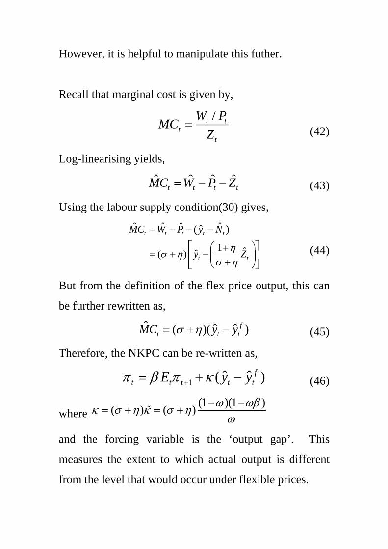
ˆt t tR vδπ= + (51)
and the policy shock following an autoregressive process
10.5t t tv v ε−= +
We adopt the parameters in Walsh Chapter 5. 0.99β = ,
1σ η= = , 1.5δ = and 0.8ω = .
Fig1 – Autoregressive Shock
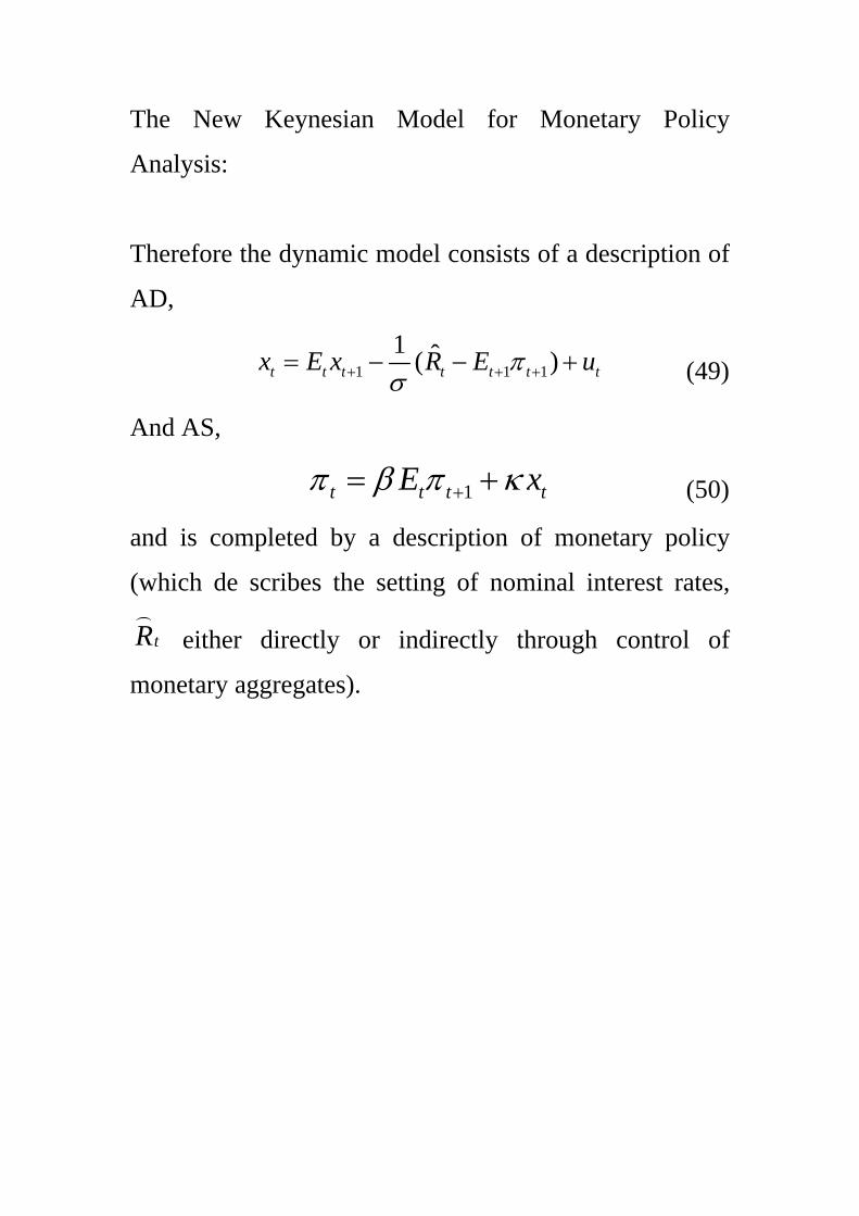
Fig 2 – iid With no autoregressive aspect to the policy
shock the movements in variables are instantaneous.
-3
-2.5
-2
-1.5
-1
-0.5
0
0.5
1
1.5
-1 0 1 2 3 4 5 6 7 8
InfRx
-1.5
-1
-0.5
0
0.5
1
1.5
-1 0 1 2 3 4 5 6 7 8
InfRx
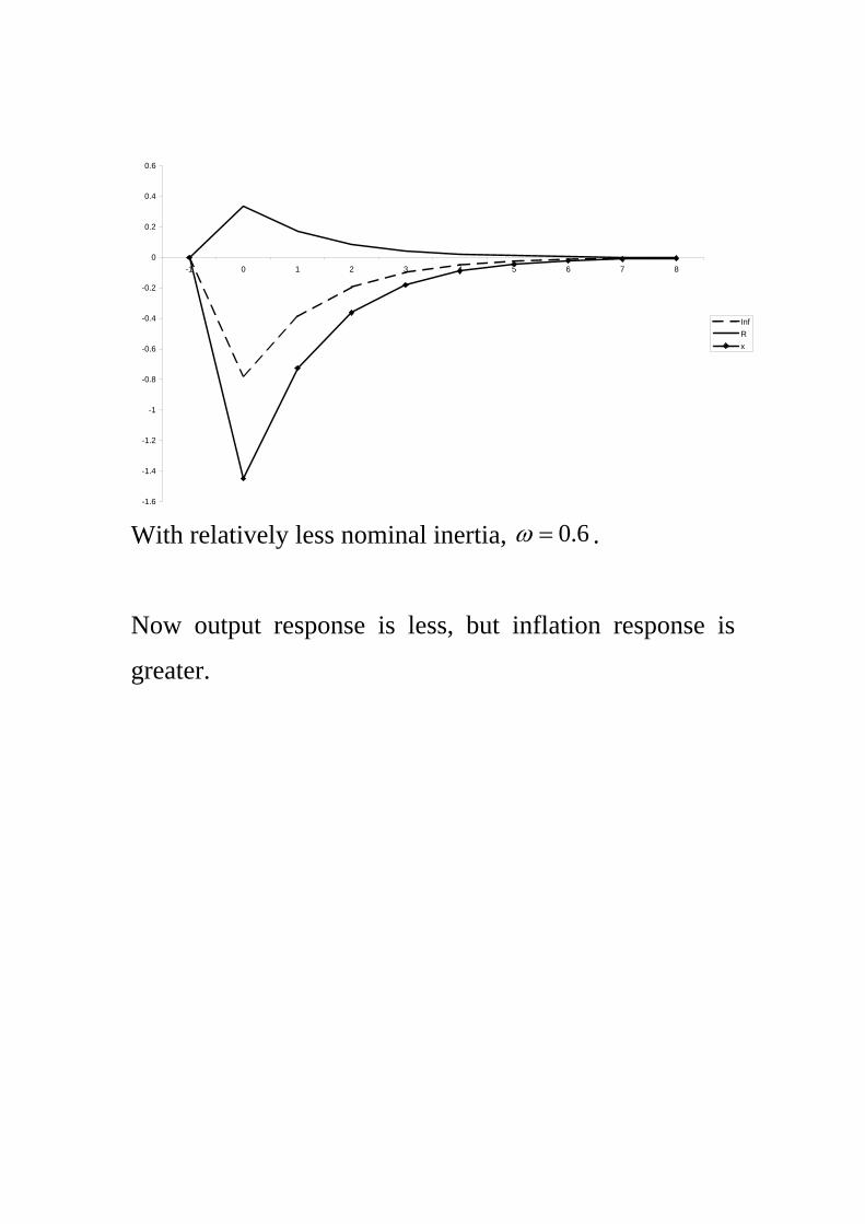
With relatively less nominal inertia, 0.6ω = .
Now output response is less, but inflation response is
greater.
-1.6
-1.4
-1.2
-1
-0.8
-0.6
-0.4
-0.2
0
0.2
0.4
0.6
-1 0 1 2 3 4 5 6 7 8
InfRx
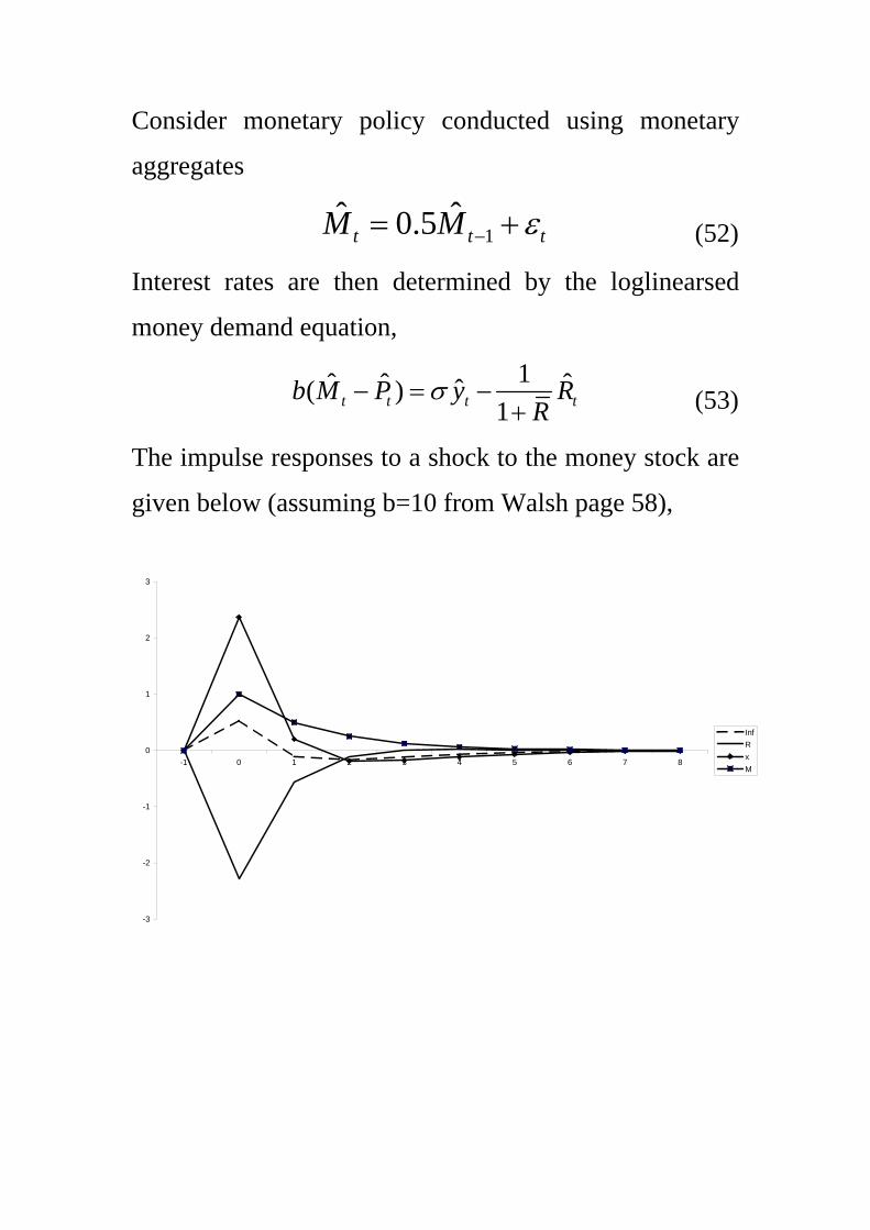
Consider monetary policy conducted using monetary
aggregates
1ˆ ˆ0.5t t tM M ε−= + (52)
Interest rates are then determined by the loglinearsed
money demand equation,
1ˆ ˆ ˆˆ( )
1t t t tb M P y RR
σ− = −+ (53)
The impulse responses to a shock to the money stock are
given below (assuming b=10 from Walsh page 58),
-3
-2
-1
0
1
2
3
-1 0 1 2 3 4 5 6 7 8
InfRxM

Policy Objectives:
Walsh considers the welfare of our representative
household can be written as,
1
0
( , ) ( ( ), )t t t t tV U Y Z v y i Z di= − ∫ (54)
where the first term represents the instantaneous utility
from consuming the consumption basket (given the level
of the productivity shock) and the second term captures
the disutility of supplying the various goods in the
economy (i.e. the disutility of labour effort is
proportional to output).

Walsh then follows Woodford (2003) to approximate the
representative household’s utility by the following
quadratic loss function,
2 * 2
0 0( )i i
t t i t t i t ii i
E V E x xβ β π λ∞ ∞
+ + += =
⎡ ⎤≈ −Ω + −⎣ ⎦∑ ∑ (55)
where
( )1 212 (1 )(1 )cYU ω θ η θ
ω ωβ−⎡ ⎤
Ω = +⎢ ⎥− −⎣ ⎦ (56)
and
(1 )(1 )
(1 )ω ωβ σ ηλ
ω ηθ θ− − +⎡ ⎤= ⎢ ⎥ +⎣ ⎦
(57)
We will not formally derive this (see Woodford(2003) or
Walsh(2003)) but it is useful to obtain some intuition for
this specification.
Recall that tx is the gap between output and the output
level that would emerge under flexible prices, and x* is
the gap between the steady-state efficient level of output
and the actual steady-state level of output.
Although this looks like a standard quadratic loss
function there are two crucial differences.
1.The output gap is measured relative to equilibrium
under flexible prices rather than the simple steady-state
output/trend output level of output.
In other words the flex price equilibrium incorporates the
optimal consumption/leisure and labour supply responses
to productivity shocks.
2.The reason for including inflation is now clear.
Sticky prices lead to a dispersion of prices and therefore
output across firms.
This has two costs for economic agents:
(1)Because of diminishing marginal utility price
dispersion has a direct utility cost (the utility gained from
consuming more of the cheaper goods is less than the
utility lost from consuming less of the expensive goods).

(2)Additionally, the cost of producing more of the cheap
goods is also typically more than the reduced costs of
producing less of the expensive goods (due to
diminishing marginal product in production, or
diminishing marginal utility of leisure if
consumers/workers are attached to specific firms).
Many authors assume that x*=0 and achieve this by
adopting some kind of fiscal subsidy to ensure that
steady-state output is at its efficient level and the
distortion due to imperfect competition has been
eliminated.
In this case the central bank’s loss function becomes,
2 2
0
( )it t i t i
i
E xβ π λ∞
+ +=
⎡ ⎤+⎣ ⎦∑ (58)
In this case we have no inflationary bias, but we do have
a stabilization bias which we illustrate below.

Optimal Policy Under Commitment
Firstly we consider optimal policy under commitment.
The bank has to minimize this loss function subject to the
structural model of the economy,
Therefore the dynamic model consists of a description of
AD,
1 1 11 ˆ( )t t t t t t tx E x R E uπσ+ + += − − + (59)
And AS,
1t t t tE xπ β π κ+= + (60)
Form the Lagrangian,
[ ]
2 21 1
0
1
1 ˆ ( ) ( )
it t i t i t i t i t i t i t i t i
i
t i t i t i t i t i
E x x x R u
x e
β π λ θ πσ
ψ π βπ κ
∞
+ + + + + + + + + +=
+ + + + + +
⎡ ⎤⎡ ⎤+ + − + − −⎣ ⎦ ⎢ ⎥⎣ ⎦+ − − −
∑
(61)

The first order condition in respect of the interest rate is
given by
1 0t t iEθσ + =
(62)
In other words, 0t t iEθ + = for i>=0 i.e. the lagrange
multiplier for the Euler equation is zero since it does not
impose any real constraint on monetary policy.
This implies that the policy could have been set up as if
the central bank controlled the output gap rather than the
interest rate (see for example Clarida et al, 1999).
Using this condition, the remaining first-order conditions
are, for inflation at time t,
0t tπ ψ+ = (63)
and for the inflation in subsequent periods,
1( ) 0t t i t i t iE π ψ ψ+ + + −+ − = (64)
and the output gap,
( ) 0t t i t iE xλ κψ+ +− = (65)

The potential time-inconsistency of policy is clear, since
in period t the central bank would set inflation equal to
t tπ ψ= − and promise to set 1 1( )t t tπ ψ ψ+ += − − .
However when period t+1 arrives the bank would wish to
set 1 1t tπ ψ+ += − .

Timelessly Optimal Policy
Woodford suggests an alternative ‘timeless perspective’
where the central bank implements (64) and (65) even in
the initial period- the bank behaves as if the policy had
always been in place. Doing this, combining the two
conditions yields,
( )1t i t i t ix xλπκ+ + + −
⎛ ⎞= − −⎜ ⎟⎝ ⎠ (66)
Summing over the infinite horizon yields,
( )10 0
t i t i t ii i
x xλπκ
∞ ∞
+ + + −= =
⎛ ⎞= − −⎜ ⎟⎝ ⎠
∑ ∑ (67)
which implies,
( )1 1p p x xλκ∞ − ∞ −
⎛ ⎞− = − −⎜ ⎟⎝ ⎠ (68)
In other words, since the output gap must eventually be
eliminated, 0x∞ = , and we can assume the initial value of
the output gap before a shock hit was also zero, 1 0x− = ,
then this means that commitment policy will ensure,
1p p∞ −= (69)
i.e. commitment policy will return the price level to its
initial value following inflationary shocks.

Policy Under Discretion:
When the central bank operates under discretion it takes
inflation expectations as given (since it cannot influence
them as it can under commitment). Therefore it has an
essentially static problem to minimize,
2 2t txπ λ+ (70)
subject to,
1t t t t tE x eπ β π κ+= + + (71)
which gives,
0t txκπ λ+ = (72)
Note that this condition is the same as the initial
condition at time t under commitment (ie. In the first
period of commitment the central bank cannot affect
initial expectations and so implements the discretionary
solution).
There is no promise on the part of the monetary
authorities to return the price level to its initial value
under discretionary policy.


Inflation response under precommitment less.
The Price Level under commitment –Pc
0
0.1
0.2
0.3
0.4
0.5
0.6
0.7
0.8
0.9
1
-1 0 1 2 3 4 5 6 7 8 9 10 11 12 13 14 15 16 17 18
Pc
-0.2
0
0.2
0.4
0.6
0.8
1
1.2
-1 0 1 2 3 4 5 6 7 8 9
infcinfd

Output fall less under commitment, but more sustained.
Inflation paths with correlated shock with coefficient of
0.9
-0.06
-0.05
-0.04
-0.03
-0.02
-0.01
0-1 0 1 2 3 4 5 6 7 8 9
xcxd
-2
0
2
4
6
8
10
12
14
16
18
-1 0 1 2 3 4 5 6 7 8 9
infcinfd

Again, output cost of stabilizing economy initially less
under commitment, but more prolonged.
There is a clear welfare improvement under commitment
given nature of loss function ( 1λ = for simplicity).
-1.8
-1.6
-1.4
-1.2
-1
-0.8
-0.6
-0.4
-0.2
0-1 0 1 2 3 4 5 6 7 8 9
xcxd
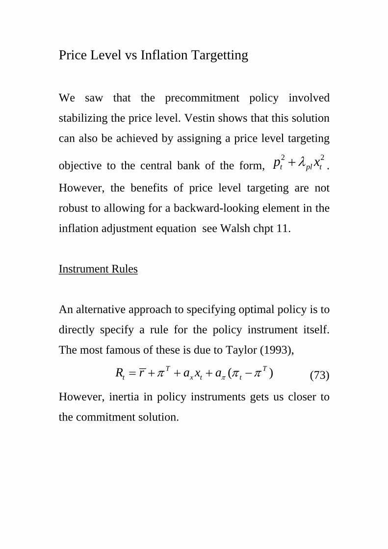
Price Level vs Inflation Targetting
We saw that the precommitment policy involved
stabilizing the price level. Vestin shows that this solution
can also be achieved by assigning a price level targeting
objective to the central bank of the form, 2 2t pl tp xλ+ .
However, the benefits of price level targeting are not
robust to allowing for a backward-looking element in the
inflation adjustment equation see Walsh chpt 11.
Instrument Rules
An alternative approach to specifying optimal policy is to
directly specify a rule for the policy instrument itself.
The most famous of these is due to Taylor (1993),
( )T Tt x t tR r a x aππ π π= + + + − (73)
However, inertia in policy instruments gets us closer to
the commitment solution.

Conclusions
• The New Keynesian Model gives a micro-founded genereal equilibrium model with sufficient nominal frictions to make monetary policy interesting.
• Its microfoundations also allow the construction of a welfare function for policy analysis which is consistent with maximising the utility of the representative consumer/worker.
• Commitment policy typically tries to make policy history dependent and in this case adopts a policy of price level targeting despite the fact that this is not an explicit objective.
• The desire to make policy history dependent may also explain the observed inertia in interest rates.