lecture 10: medical image segmentation as an …bagci/teaching/mic17/lec10.pdf• each pixel = node...
TRANSCRIPT
MEDICAL IMAGE COMPUTING (CAP 5937)
LECTURE 10: Medical Image Segmentation as an Energy Minimization Problem
Dr. Ulas BagciHEC 221, Center for Research in Computer Vision (CRCV), University of Central Florida (UCF), Orlando, FL [email protected] or [email protected]
1SPRING 2017
Outline• Energy functional
– Data and Smoothness terms• Graph Cut
– Min cut– Max Flow
• Applications in Radiology Images
2

Motivation 3
Manual annotation through expert raters. Shown are image patches with the tumor structures that are annotated in the different modalities (top left) and the final labels for the whole dataset (right). Image patches show from left to right: the whole tumor visible in FLAIR (A), the tumor core visible in T2 (B), the enhancing tumor structures visible in T1c (blue), surrounding the cystic/necrotic components of the core (green) (C). Segmentations are combined to generate the final labels of the tumor structures (D): edema (yellow), non-enhancing solid core (red), necrotic/cystic core (green), enhancing core(blue). Credit: BRATS paper/TMI

Labeling & Segmentation• Labeling is a common way for modeling various computer
vision problems (e.g. optical flow, image segmentation, stereo matching, etc)
4

Labeling & Segmentation• Labeling is a common way for modeling various computer
vision problems (e.g. optical flow, image segmentation, stereo matching, etc)
• The set of labels can be discrete (as in image segmentation)
5
L = {l1, . . . , lm} with L = m

Labeling & Segmentation• Labeling is a common way for modeling various computer
vision problems (e.g. optical flow, image segmentation, stereo matching, etc)
• The set of labels can be discrete (as in image segmentation)
• Or continuous (tracking, etc.)
6
L = {l1, . . . , lm} with L = m
L ⇢ Rnfor n � 1

Labeling is a function• Labels are assigned to sites (pixel locations)
7

Labeling is a function• Labels are assigned to sites (pixel locations)• For a given image, we have
8
|⌦| = Ncols
.Nrows

Labeling is a function• Labels are assigned to sites (pixel locations)• For a given image, we have• Identifying a labeling function (with segmentation) is
9
|⌦| = Ncols
.Nrows
f : ⌦ ! L

Labeling is a function• Labels are assigned to sites (pixel locations)• For a given image, we have• Identifying a labeling function (with segmentation) is
We aim at calculating a labeling function that minimizes a given (total) error or energy
10
|⌦| = Ncols
.Nrows
f : ⌦ ! L

Labeling is a function• Labels are assigned to sites (pixel locations)• For a given image, we have• Identifying a labeling function (with segmentation) is
We aim at calculating a labeling function that minimizes a given (total) error or energy
11
|⌦| = Ncols
.Nrows
f : ⌦ ! L
E(f) =X
p2⌦
[Edata
(p, fp
) +X
q2A(p)
Esmooth
(fp
, fq
)]
*A is an adjacency relation between pixel locations

Example of Energy Minimization Methods
12
Credit: Zhao et al., IJNMBE 15

Energy Function?• Penalizing results which are not compatible with the
observed images/volumes
13

Energy Function?• Penalizing results which are not compatible with the
observed images/volumes
14
Unary (data) cost (inverted)

Energy Function?• Penalizing results which are not compatible with the
observed images/volumes• Enforcing spatial coherence.
15
Pairwise (boundary) cost (inverted)

Energy Function?• Penalizing results which are not compatible with the
observed images/volumes• Enforcing spatial coherence.
16
Pairwise (boundary) cost (inverted)
p q
Segmentation as an Energy Minimization Problem• Edata assigns non-negative penalties to a pixel location p
when assigning a label to this location.
10/1/15
17

Segmentation as an Energy Minimization Problem• Edata assigns non-negative penalties to a pixel location p
when assigning a label to this location.• Esmooth assigns non-negative penalties by comparing the
assigned labels fp and fq at adjacent positions p and q.
18
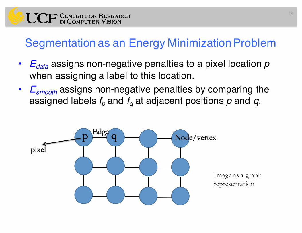
Segmentation as an Energy Minimization Problem• Edata assigns non-negative penalties to a pixel location p
when assigning a label to this location.• Esmooth assigns non-negative penalties by comparing the
assigned labels fp and fq at adjacent positions p and q.
19
Node/vertexEdge
pixel
p q
Image as a graphrepresentation

Segmentation as an Energy Minimization Problem• Edata assigns non-negative penalties to a pixel location p
when assigning a label to this location.• Esmooth assigns non-negative penalties by comparing the
assigned labels fp and fq at adjacent positions p and q.
20
This optimization model is characterized by local interactions along edges between adjacent pixels, and often called MRF (Markov Random Field) model.

Energy Function-Details
21
E(f) =X
p2⌦
[Edata
(p, fp
) +X
q2A(p)
Esmooth
(fp
, fq
)]

Energy Function-Details
22
E(f) =X
p2⌦
[Edata
(p, fp
) +X
q2A(p)
Esmooth
(fp
, fq
)]
Edata(p, fp) = (p)
(p = 0) = �logP (p 2 BG)
(p = 1) = �logP (p 2 FG)
Example Data Term:

Energy Function-Details
23
E(f) =X
p2⌦
[Edata
(p, fp
) +X
q2A(p)
Esmooth
(fp
, fq
)]
Edata(p, fp) = (p)
(p = 0) = �logP (p 2 BG)
(p = 1) = �logP (p 2 FG)
Example Data Term:
(p, q) = Kpq�(p 6= q) where
Kpq =exp(��(Ip � Iq)2/(2�2))
||p, q||
Example Smoothness Term:

Energy Function-Details
24
E(f) =X
p2⌦
[Edata
(p, fp
) +X
q2A(p)
Esmooth
(fp
, fq
)]
E(p) =X
p2⌦
p(p) +X
p2⌦
X
q2A(p)
pq(p, q)
p⇤ = argminp2L
E(p)

Energy Function-Details
25
E(f) =X
p2⌦
[Edata
(p, fp
) +X
q2A(p)
Esmooth
(fp
, fq
)]
E(p) =X
p2⌦
p(p) +X
p2⌦
X
q2A(p)
pq(p, q)
p⇤ = argminp2L
E(p)
To solve this problem, transform the energy functional into min-cut/max-flow problem and solve it!

Graph Cuts for Optimal Boundary Detection (Boykov ICCV 2001)
26
26
F
B
F
B
F
F F
F B
B
B
• Binary label: foreground vs. background• User labels some pixels • Exploit
– Statistics of known Fg & Bg– Smoothness of label
• Turn into discrete graph optimization– Graph cut (min cut / max flow)
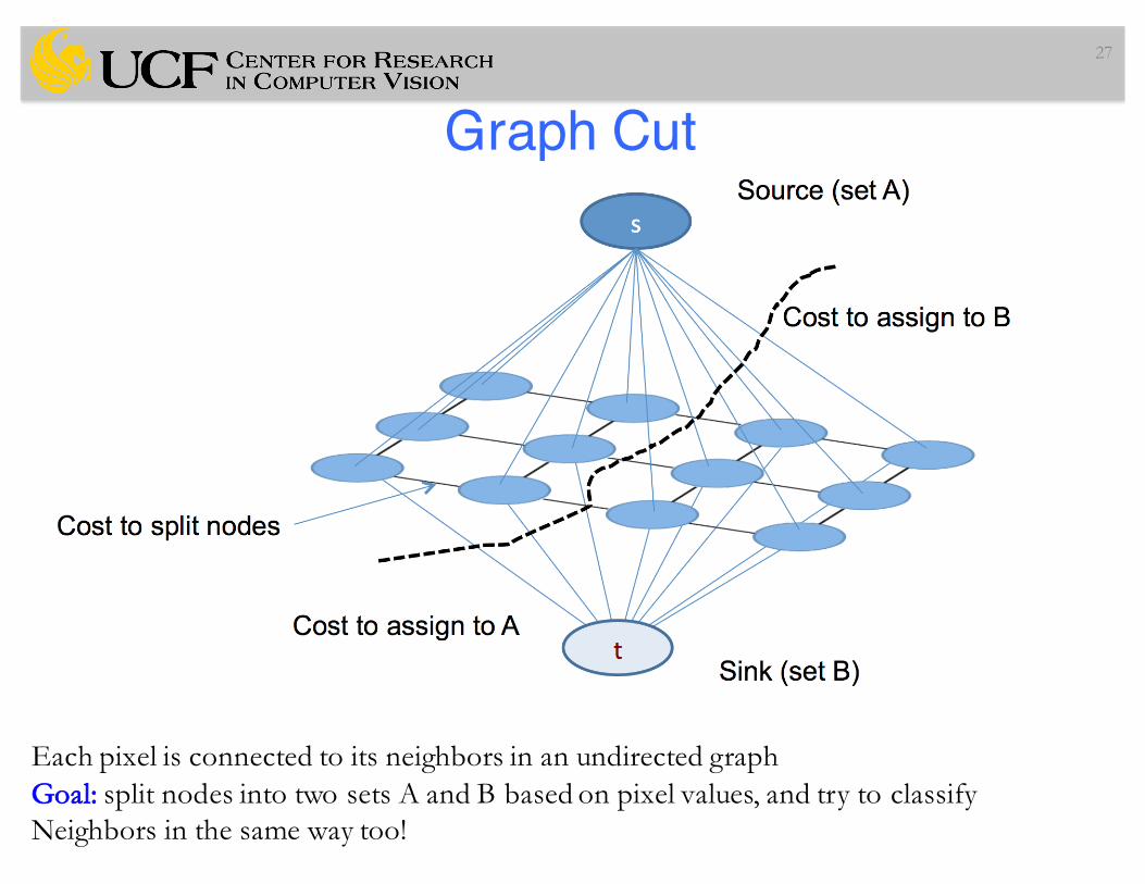
Graph Cut27
Each pixel is connected to its neighbors in an undirected graphGoal: split nodes into two sets A and B based on pixel values, and try to classify Neighbors in the same way too!

Graph Cut28
Each pixel is connected to its neighbors in an undirected graphGoal: split nodes into two sets A and B based on pixel values, and try to classify Neighbors in the same way too!

Graph-Cut29
• Each pixel = node• Add two nodes F & B• Labeling: link each pixel to either F or B
F
B
F
B
F
F F
F B
B
B
Desired result

Cost Function: Data term
30
• Put one edge between each pixel and both F & G• Weight of edge = minus data term
B
F

Cost Function: Smoothness term31
• Add an edge between each neighbor pair• Weight = smoothness term
B
F

Min-Cut32
• Energy optimization equivalent to graph min cut• Cut: remove edges to disconnect F from B• Minimum: minimize sum of cut edge weight
B
Fcut
Min-Cut33
Source
Sink
v1 v2
2
5
9
42
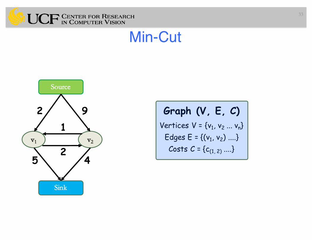
1Graph (V, E, C)
Vertices V = {v1, v2 ... vn}Edges E = {(v1, v2) ....}Costs C = {c(1, 2) ....}

Min-Cut34
Source
Sink
v1 v2
2
5
9
42
1
What is a st-cut?
An st-cut (S,T) divides the nodes between source and sink.
What is the cost of a st-cut?
Sum of cost of all edges going from S to T
5 + 2 + 9 = 16

Min-Cut35
What is a st-cut?
An st-cut (S,T) divides the nodes between source and sink.
What is the cost of a st-cut?
Sum of cost of all edges going from S to T
Source
Sink
v1 v2
2
5
9
42
1
2 + 1 + 4 = 7
What is the st-mincut?
st-cut with the minimum cost

How to compute min-cut?36
Source
Sink
v1 v2
2
5
9
42
1
Solve the dual maximum flow problem
In every network, the maximum flow equals the cost of the st-mincut
Min-cut\Max-flow Theorem
Compute the maximum flow between Source and Sink
Constraints
Edges: Flow < Capacity
Nodes: Flow in & Flow out

Max-Flow Algorithms
37
Augmenting Path Based Algorithms
1. Find path from source to sink with positive capacity
2. Push maximum possible flow through this path
3. Repeat until no path can be found
Source
Sink
v1 v2
2
5
9
42
1
Algorithms assume non-negative capacity
Flow=0
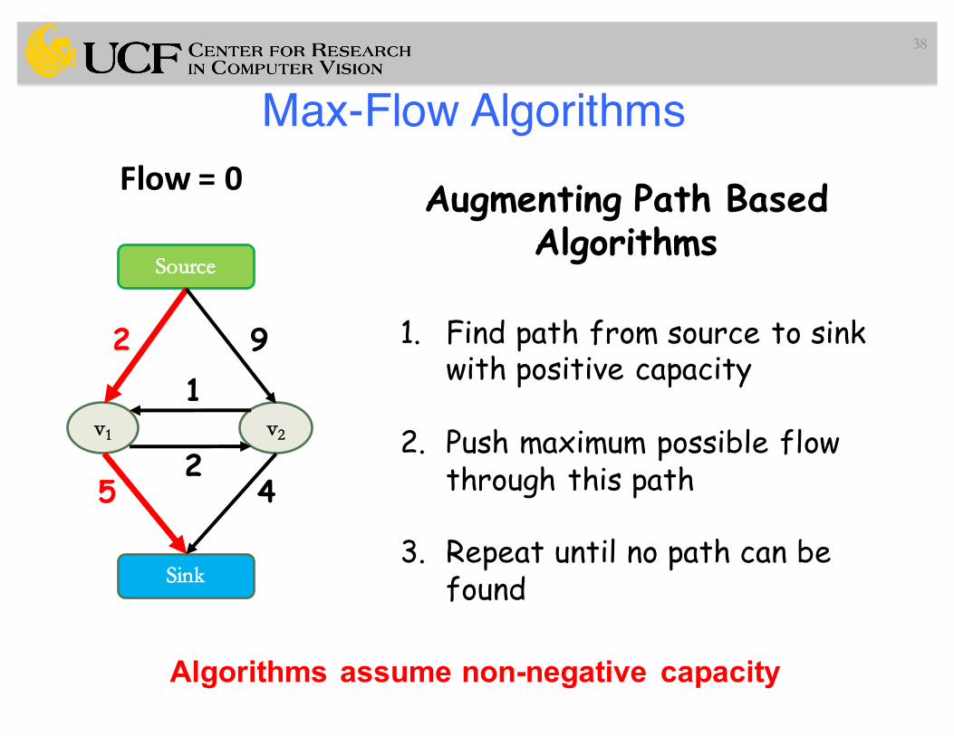
Max-Flow Algorithms38
Augmenting Path Based Algorithms
1. Find path from source to sink with positive capacity
2. Push maximum possible flow through this path
3. Repeat until no path can be found
Algorithms assume non-negative capacity
Source
Sink
v1 v2
2
5
9
42
1
Flow=0

Max-Flow Algorithms
39
Augmenting Path Based Algorithms
1. Find path from source to sink with positive capacity
2. Push maximum possible flow through this path
3. Repeat until no path can be found
Algorithms assume non-negative capacity
Source
Sink
v1 v2
2-2
5-2
9
42
1
Flow=0+2

Max-Flow Algorithms
40
Augmenting Path Based Algorithms
1. Find path from source to sink with positive capacity
2. Push maximum possible flow through this path
3. Repeat until no path can be found
Algorithms assume non-negative capacity
Source
Sink
v1 v2
0
3
9
42
1
Flow=2

Max-Flow Algorithms
41
Augmenting Path Based Algorithms
1. Find path from source to sink with positive capacity
2. Push maximum possible flow through this path
3. Repeat until no path can be found
Algorithms assume non-negative capacity
Source
Sink
v1 v2
0
3
9
42
1
Flow=2

Max-Flow Algorithms
42
Augmenting Path Based Algorithms
1. Find path from source to sink with positive capacity
2. Push maximum possible flow through this path
3. Repeat until no path can be found
Algorithms assume non-negative capacity
Source
Sink
v1 v2
0
3
9
42
1
Flow=2

Max-Flow Algorithms
43
Augmenting Path Based Algorithms
1. Find path from source to sink with positive capacity
2. Push maximum possible flow through this path
3. Repeat until no path can be found
Algorithms assume non-negative capacity
Source
Sink
v1 v2
0
3
5
02
1
Flow=2+4

Max-Flow Algorithms
44
Augmenting Path Based Algorithms
1. Find path from source to sink with positive capacity
2. Push maximum possible flow through this path
3. Repeat until no path can be found
Algorithms assume non-negative capacity
Source
Sink
v1 v2
0
3
5
02
1
Flow=6

Max-Flow Algorithms
45
Augmenting Path Based Algorithms
1. Find path from source to sink with positive capacity
2. Push maximum possible flow through this path
3. Repeat until no path can be found
Algorithms assume non-negative capacity
Source
Sink
v1 v2
0
3
5
02
1
Flow=6

Max-Flow Algorithms
46
Augmenting Path Based Algorithms
1. Find path from source to sink with positive capacity
2. Push maximum possible flow through this path
3. Repeat until no path can be found
Algorithms assume non-negative capacity
Source
Sink
v1 v2
0
2
4
02+1
1-1
Flow=6+1

Max-Flow Algorithms
47
Augmenting Path Based Algorithms
1. Find path from source to sink with positive capacity
2. Push maximum possible flow through this path
3. Repeat until no path can be found
Algorithms assume non-negative capacity
Source
Sink
v1 v2
0
2
4
03
0
Flow=7
Max-Flow Algorithms
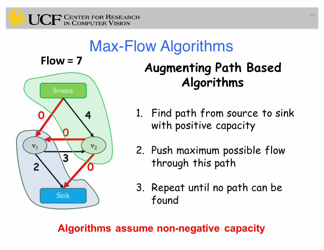
48
Augmenting Path Based Algorithms
1. Find path from source to sink with positive capacity
2. Push maximum possible flow through this path
3. Repeat until no path can be found
Algorithms assume non-negative capacity
Source
Sink
v1 v2
0
2
4
03
0
Flow=7

Another Example-Max Flow
49
source
sink
9
5
6
8
42
2
2
5
3
5
5
311
6
2
3
Ford & Fulkerson algorithm (1956)
Find the path from source to sink
While (path exists)
flow += maximum capacity in the path
Build the residual graph (“subtract” the flow)
Find the path in the residual graph
End

Another Example-Max Flow
50
source
sink
9
5
6
8
42
2
2
5
3
5
5
311
6
2
3
Ford & Fulkerson algorithm (1956)
Find the path from source to sink
While (path exists)
flow += maximum capacity in the path
Build the residual graph (“subtract” the flow)
Find the path in the residual graph
End

Another Example-Max Flow
51
source
sink
9
5
6
8
42
2
2
5
3
5
5
311
6
2
3
Ford & Fulkerson algorithm (1956)
Find the path from source to sink
While (path exists)
flow += maximum capacity in the path
Build the residual graph (“subtract” the flow)
Find the path in the residual graph
End
flow = 3

Another Example-Max Flow
52
source
sink
9
5
6-3
8-3
42+3
2
2
5-3
3-3
5
5
311
6
2
3
Ford & Fulkerson algorithm (1956)
Find the path from source to sink
While (path exists)
flow += maximum capacity in the path
Build the residual graph (“subtract” the flow)
Find the path in the residual graph
End
flow = 3
+3

Another Example-Max Flow
53
source
sink
9
5
3
5
45
2
2
2
5
5
311
6
2
3
Ford & Fulkerson algorithm (1956)
Find the path from source to sink
While (path exists)
flow += maximum capacity in the path
Build the residual graph (“subtract” the flow)
Find the path in the residual graph
End
flow = 3
3

Another Example-Max Flow
54
source
sink
9
5
3
5
45
2
2
2
5
5
311
6
2
3
Ford & Fulkerson algorithm (1956)
Find the path from source to sink
While (path exists)
flow += maximum capacity in the path
Build the residual graph (“subtract” the flow)
Find the path in the residual graph
End
flow = 3
3

Another Example-Max Flow
55
source
sink
9
5
3
5
45
2
2
2
5
5
311
6
2
3
Ford & Fulkerson algorithm (1956)
Find the path from source to sink
While (path exists)
flow += maximum capacity in the path
Build the residual graph (“subtract” the flow)
Find the path in the residual graph
End
flow = 6
3

Another Example-Max Flow
56
source
sink
9-3
5
3
5-3
45
2
2
2
5
5
3-311
6
2
3-3
Ford & Fulkerson algorithm (1956)
Find the path from source to sink
While (path exists)
flow += maximum capacity in the path
Build the residual graph (“subtract” the flow)
Find the path in the residual graph
End
flow = 6
3
+3
+3

Another Example-Max Flow
57
source
sink
6
5
3
2
45
2
2
2
5
5
11
6
2
Ford & Fulkerson algorithm (1956)
Find the path from source to sink
While (path exists)
flow += maximum capacity in the path
Build the residual graph (“subtract” the flow)
Find the path in the residual graph
End
flow = 6
3
3
3
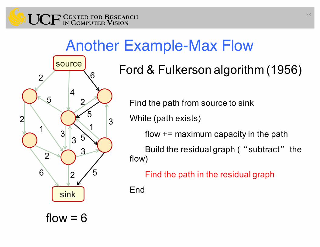
Another Example-Max Flow
58
source
sink
6
5
3
2
45
2
2
2
5
5
11
6
2
Ford & Fulkerson algorithm (1956)
Find the path from source to sink
While (path exists)
flow += maximum capacity in the path
Build the residual graph (“subtract” the flow)
Find the path in the residual graph
End
flow = 6
3
3
3

Another Example-Max Flow
59
source
sink
6
5
3
2
45
2
2
2
5
5
11
6
2
Ford & Fulkerson algorithm (1956)
Find the path from source to sink
While (path exists)
flow += maximum capacity in the path
Build the residual graph (“subtract” the flow)
Find the path in the residual graph
End
flow = 11
3
3
3

Another Example-Max Flow
60
source
sink
6-5
5-5
3
2
45
2
2
2
5-5
5-5
1+51
6
2+5
Ford & Fulkerson algorithm (1956)
Find the path from source to sink
While (path exists)
flow += maximum capacity in the path
Build the residual graph (“subtract” the flow)
Find the path in the residual graph
End
flow = 11
3
3
3

Another Example-Max Flow
61
source
sink
1
3
2
45
2
2
2
61
6
7
Ford & Fulkerson algorithm (1956)
Find the path from source to sink
While (path exists)
flow += maximum capacity in the path
Build the residual graph (“subtract” the flow)
Find the path in the residual graph
End
flow = 11
3
33

Another Example-Max Flow
62
source
sink
1
3
2
45
2
2
2
61
6
7
Ford & Fulkerson algorithm (1956)
Find the path from source to sink
While (path exists)
flow += maximum capacity in the path
Build the residual graph (“subtract” the flow)
Find the path in the residual graph
End
flow = 11
3
33

Another Example-Max Flow
63
source
sink
1
3
2
45
2
2
2
61
6
7
Ford & Fulkerson algorithm (1956)
Find the path from source to sink
While (path exists)
flow += maximum capacity in the path
Build the residual graph (“subtract” the flow)
Find the path in the residual graph
End
flow = 13
3
33

Another Example-Max Flow
64
source
sink
1
3
2-2
45
2-2
2-2
2-2
61
6
7
Ford & Fulkerson algorithm (1956)
Find the path from source to sink
While (path exists)
flow += maximum capacity in the path
Build the residual graph (“subtract” the flow)
Find the path in the residual graph
End
flow = 13
3
33
+2
+2

Another Example-Max Flow
65
source
sink
1
3
45
61
6
7
Ford & Fulkerson algorithm (1956)
Find the path from source to sink
While (path exists)
flow += maximum capacity in the path
Build the residual graph (“subtract” the flow)
Find the path in the residual graph
End
flow = 13
3
33
2
2

Another Example-Max Flow
66
source
sink
1
3
45
61
6
7
Ford & Fulkerson algorithm (1956)
Find the path from source to sink
While (path exists)
flow += maximum capacity in the path
Build the residual graph (“subtract” the flow)
Find the path in the residual graph
End
flow = 13
3
33
2
2

Another Example-Max Flow
67
source
sink
1
3
45
61
6
7
Ford & Fulkerson algorithm (1956)
Find the path from source to sink
While (path exists)
flow += maximum capacity in the path
Build the residual graph (“subtract” the flow)
Find the path in the residual graph
End
flow = 15
3
33
2
2

Another Example-Max Flow
68
source
sink
1
3-2
4-25
61
6-2
7
Ford & Fulkerson algorithm (1956)
Find the path from source to sink
While (path exists)
flow += maximum capacity in the path
Build the residual graph (“subtract” the flow)
Find the path in the residual graph
End
flow = 15
3
33+2
2
2-2
+2
Another Example-Max Flow
69
source
sink
1
1
5
61
4
7
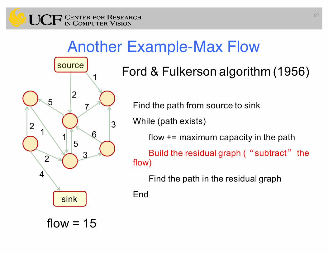
Ford & Fulkerson algorithm (1956)
Find the path from source to sink
While (path exists)
flow += maximum capacity in the path
Build the residual graph (“subtract” the flow)
Find the path in the residual graph
End
flow = 15
3
35
2
2
2

Another Example-Max Flow
70
source
sink
1
1
5
61
4
7
Ford & Fulkerson algorithm (1956)
Find the path from source to sink
While (path exists)
flow += maximum capacity in the path
Build the residual graph (“subtract” the flow)
Find the path in the residual graph
End
flow = 15
3
35
2
2
2

Another Example-Max Flow
71
source
sink
1
1
5
61
4
7
Ford & Fulkerson algorithm (1956)
Find the path from source to sink
While (path exists)
flow += maximum capacity in the path
Build the residual graph (“subtract” the flow)
Find the path in the residual graph
End
flow = 15
3
35
2
2
2

Another Example-Max Flow
72
source
sink
1
1
5
61
4
7
Ford & Fulkerson algorithm (1956)
Why is the solution globally optimal ?
flow = 15
3
35
2
2
2

Another Example-Max Flow
73
source
sink
1
1
5
61
4
7
Ford & Fulkerson algorithm (1956)
Why is the solution globally optimal ?
1. Let S be the set of reachable nodes in the
residual graph
flow = 15
3
35
2
2
2
S
Another Example-Max Flow
74
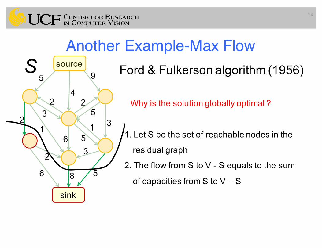
Ford & Fulkerson algorithm (1956)
Why is the solution globally optimal ?
1. Let S be the set of reachable nodes in the
residual graph
2. The flow from S to V - S equals to the sum
of capacities from S to V – S
source
sink
9
5
6
8
42
2
2
5
3
5
5
311
6
2
3
S

Another Example-Max Flow
75
flow = 15
Ford & Fulkerson algorithm (1956)
Why is the solution globally optimal ?
1. Let S be the set of reachable nodes in the residual graph
2. The flow from S to V - S equals to the sum of capacities from S to V – S
3. The flow from any A to V - A is upper bounded by the sum of capacities from A to V – A
4. The solution is globally optimal
source
sink
8/9
5/5
5/6
8/8
2/40/2
2/2
0/2
5/5
3/3
5/5
5/5
3/30/10/1
2/6
0/2
3/3
Individual flows obtained by summing up all paths

Another Example-Max Flow
76
source
sink
9
5
6
8
42
2
2
5
3
5
5
311
6
2
3
S
T
cost = 18
source
sink
9
5
6
8
42
2
2
5
3
5
5
311
6
2
3
S
T

Another Example-Max Flow
77
source
sink
9
5
6
8
42
2
2
5
3
5
5
311
6
2
3
S
T
cost = 23

Another Example-Max Flow
78
C(x) = 5x1 + 9x2 + 4x3 + 3x3(1-x1) + 2x1(1-x3)
+ 3x3(1-x1) + 2x2(1-x3) + 5x3(1-x2) + 2x4(1-x1)
+ 1x5(1-x1) + 6x5(1-x3) + 5x6(1-x3) + 1x3(1-x6)
+ 3x6(1-x2) + 2x4(1-x5) + 3x6(1-x5) + 6(1-x4)
+ 8(1-x5) + 5(1-x6)
source
sink
9
5
6
8
42
2
2
5
3
5
5
311
6
2
3
x1 x2
x3
x4
x5
x6

Another Example-Max Flow
79
C(x) = 2x1 + 9x2 + 4x3 + 2x1(1-x3)
+ 3x3(1-x1) + 2x2(1-x3) + 5x3(1-x2) + 2x4(1-x1)
+ 1x5(1-x1) + 3x5(1-x3) + 5x6(1-x3) + 1x3(1-x6)
+ 3x6(1-x2) + 2x4(1-x5) + 3x6(1-x5) + 6(1-x4)
+ 5(1-x5) + 5(1-x6)
+ 3x1 + 3x3(1-x1) + 3x5(1-x3) + 3(1-x5)
source
sink
9
5
6
8
42
2
2
5
3
5
5
311
6
2
3
x1 x2
x3
x4
x5
x6

Another Example-Max Flow
80
C(x) = 2x1 + 9x2 + 4x3 + 2x1(1-x3)
+ 3x3(1-x1) + 2x2(1-x3) + 5x3(1-x2) + 2x4(1-x1)
+ 1x5(1-x1) + 3x5(1-x3) + 5x6(1-x3) + 1x3(1-x6)
+ 3x6(1-x2) + 2x4(1-x5) + 3x6(1-x5) + 6(1-x4)
+ 5(1-x5) + 5(1-x6)
+ 3x1 + 3x3(1-x1) + 3x5(1-x3) + 3(1-x5)
3x1 + 3x3(1-x1) + 3x5(1-x3) + 3(1-x5)
=
3 + 3x1(1-x3) + 3x3(1-x5)
source
sink
9
5
6
8
42
2
2
5
3
5
5
311
6
2
3
x1 x2
x3
x4
x5
x6

Another Example-Max Flow
81
C(x) = 3 + 2x1 + 6x2 + 4x3 + 5x1(1-x3)
+ 3x3(1-x1) + 2x2(1-x3) + 5x3(1-x2) + 2x4(1-x1)
+ 1x5(1-x1) + 3x5(1-x3) + 5x6(1-x3) + 1x3(1-x6)
+ 2x5(1-x4) + 6(1-x4)
+ 2(1-x5) + 5(1-x6) + 3x3(1-x5)
+ 3x2 + 3x6(1-x2) + 3x5(1-x6) + 3(1-x5)
3x2 + 3x6(1-x2) + 3x5(1-x6) + 3(1-x5)
=
3 + 3x2(1-x6) + 3x6(1-x5)
source
sink
9
5
3
5
45
2
2
2
5
5
311
6
2
33
x1 x2
x3
x4
x5
x6
82
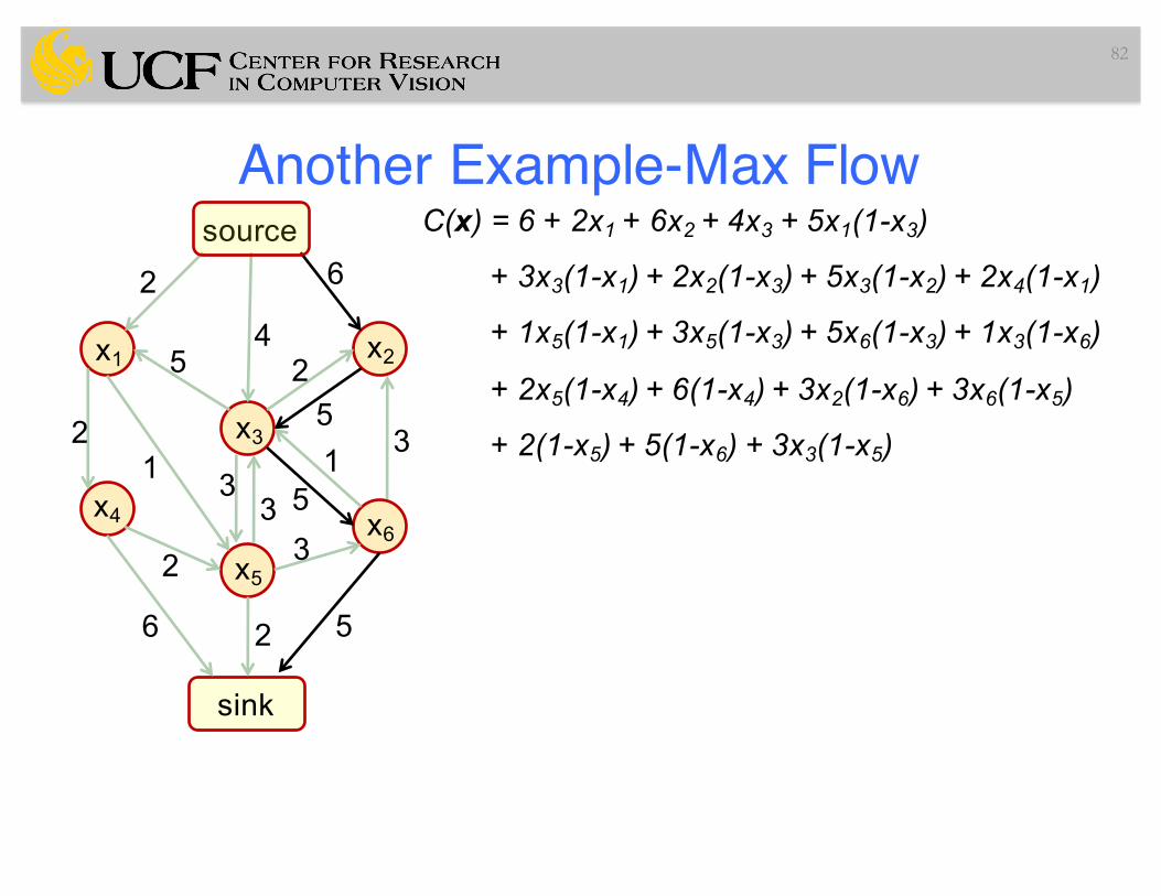
C(x) = 6 + 2x1 + 6x2 + 4x3 + 5x1(1-x3)
+ 3x3(1-x1) + 2x2(1-x3) + 5x3(1-x2) + 2x4(1-x1)
+ 1x5(1-x1) + 3x5(1-x3) + 5x6(1-x3) + 1x3(1-x6)
+ 2x5(1-x4) + 6(1-x4) + 3x2(1-x6) + 3x6(1-x5)
+ 2(1-x5) + 5(1-x6) + 3x3(1-x5)
source
sink
6
5
3
2
45
2
2
2
5
5
11
6
2
3
3
3
x1 x2
x3
x4
x5
x6
Another Example-Max Flow

Another Example-Max Flow83
C(x) = 15 + 1x2 + 4x3 + 5x1(1-x3)
+ 3x3(1-x1) + 7x2(1-x3) + 2x1(1-x4)
+ 1x5(1-x1) + 6x3(1-x6) + 6x3(1-x5)
+ 2x5(1-x4) + 4(1-x4) + 3x2(1-x6) + 3x6(1-x5)
source
sink
1
1
5
61
4
7
3
35
2
2
2x1 x2
x3
x4
x5
x6 cost = 0
min cut
S
T
cost = 0
• All coefficients positive
• Must be global minimum
S – set of reachable nodes from s

History of Max-Flow Algorithms84
Augmenting Path and Push-Relabeln: #nodesm: #edgesU: maximum edge weight
Algorithms assume non-negative edge
weights
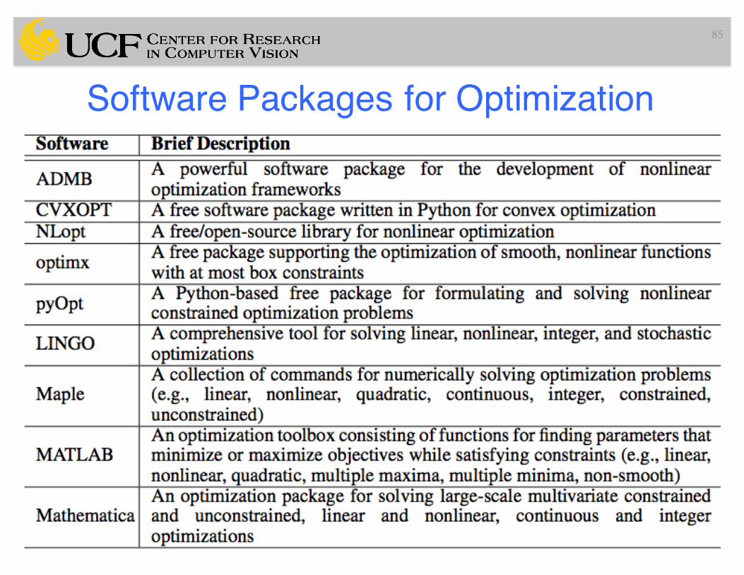
Software Packages for Optimization
85

Applications Used in Energy Minimization Based Segmentation Methods
86

Applications
87

Interactive Organ Segmentation (Boykov and Jolly, MICCAI 2000)
88
Segmentation of multiple objects. (a-c): Cardiac MRI. (d): Kidney CE-MR angiography

Interactive Organ Segmentation (Boykov and Jolly, MICCAI 2000)
89
Segmentation of the right lung in CT. (a): representative 2D slice of original 3D data. (b): segmentation results on the slice in (a). (c-d) 3D visualization of segmentation results.

AUTOMATIC HEART ISOLATION FOR CT CORONARY VISUALIZATION USING GRAPH-CUTS (Funka-Lea et al, ISBI 2006)
• Isolating the entire heart allows the coronary vessels on the surface of the heart to be easily visualized despite the proximity of surrounding organs such as the ribs and pulmonary blood vessels.
90

AUTOMATIC HEART ISOLATION FOR CT CORONARY VISUALIZATION USING GRAPH-CUTS (Funka-Lea et al, ISBI 2006)
• Isolating the entire heart allows the coronary vessels on the surface of the heart to be easily visualized despite the proximity of surrounding organs such as the ribs and pulmonary blood vessels.
• Numerous techniques have been described for segmenting the left ventricle of the heart in images from various types of medical scanners but rarely has the entire heart been segmented.
91

AUTOMATIC HEART ISOLATION FOR CT CORONARY VISUALIZATION USING GRAPH-CUTS (Funka-Lea et al, ISBI 2006)
• Isolating the entire heart allows the coronary vessels on the surface of the heart to be easily visualized despite the proximity of surrounding organs such as the ribs and pulmonary blood vessels.
• Numerous techniques have been described for segmenting the left ventricle of the heart in images from various types of medical scanners but rarely has the entire heart been segmented.
• Graph-cut formation:
92

AUTOMATIC HEART ISOLATION FOR CT CORONARY VISUALIZATION USING GRAPH-CUTS (Funka-Lea et al, ISBI 2006)
• Isolating the entire heart allows the coronary vessels on the surface of the heart to be easily visualized despite the proximity of surrounding organs such as the ribs and pulmonary blood vessels.
• Numerous techniques have been described for segmenting the left ventricle of the heart in images from various types of medical scanners but rarely has the entire heart been segmented.
• Graph-cut formation:
93

AUTOMATIC HEART ISOLATION FOR CT CORONARY VISUALIZATION USING GRAPH-CUTS (Funka-Lea et al, ISBI 2006)
• Isolating the entire heart allows the coronary vessels on the surface of the heart to be easily visualized despite the proximity of surrounding organs such as the ribs and pulmonary blood vessels.
• Numerous techniques have been described for segmenting the left ventricle of the heart in images from various types of medical scanners but rarely has the entire heart been segmented.
• Graph-cut formation:
94
(C is center)

AUTOMATIC HEART ISOLATION FOR CT CORONARY VISUALIZATION USING GRAPH-CUTS (Funka-Lea et al, ISBI 2006)
• Isolating the entire heart allows the coronary vessels on the surface of the heart to be easily visualized despite the proximity of surrounding organs such as the ribs and pulmonary blood vessels.
• Numerous techniques have been described for segmenting the left ventricle of the heart in images from various types of medical scanners but rarely has the entire heart been segmented.
• Graph-cut formation:
95
If cos(.) <0, (0 otherwise.)
(C is center)

AUTOMATIC HEART ISOLATION FOR CT CORONARY VISUALIZATION USING GRAPH-CUTS (Funka-Lea et al, ISBI 2006)
96
Top Left:A balloon is expanded within the heart. The heart wall pushes the balloon toward the heart center as the balloon grows.
Top right: volume rendering of original heart volume.
Bottom left: heart cropped based on segmentation mask.
Bottom right:volume rendering after automatic heart isolation algorithm.

Measurement of hippocampal atrophy using 4D graph-cut segmentation: Application to ADNI (Wolz, et al. NeuroImage 10)
• Proposed a method for simultaneously segmenting longitudinal magnetic resonance (MR) images
97

Measurement of hippocampal atrophy using 4D graph-cut segmentation: Application to ADNI (Wolz, et al. NeuroImage 10)
• Proposed a method for simultaneously segmenting longitudinal magnetic resonance (MR) images– 3D MRI + time component (longitudinal)
98

Measurement of hippocampal atrophy using 4D graph-cut segmentation: Application to ADNI (Wolz, et al. NeuroImage 10)
• Proposed a method for simultaneously segmenting longitudinal magnetic resonance (MR) images– 3D MRI + time component (longitudinal)
• A 4D graph is used to represent the longitudinal data: – edges are weighted based on spatial and intensity priors and connect
spatially and temporally neighboring voxels represented by vertices in the graph.
99

Measurement of hippocampal atrophy using 4D graph-cut segmentation: Application to ADNI (Wolz, et al. NeuroImage 10)
• Proposed a method for simultaneously segmenting longitudinal magnetic resonance (MR) images– 3D MRI + time component (longitudinal)
• A 4D graph is used to represent the longitudinal data: – edges are weighted based on spatial and intensity priors and connect
spatially and temporally neighboring voxels represented by vertices in the graph.
– Solving the min-cut/max-flow problem on this graph yields the segmentation for all time-points in a single step
100

Measurement of hippocampal atrophy using 4D graph-cut segmentation: Application to ADNI (Wolz, et al. NeuroImage 10)
• Proposed a method for simultaneously segmenting longitudinal magnetic resonance (MR) images– 3D MRI + time component (longitudinal)
• A 4D graph is used to represent the longitudinal data: – edges are weighted based on spatial and intensity priors and connect
spatially and temporally neighboring voxels represented by vertices in the graph.
– Solving the min-cut/max-flow problem on this graph yields the segmentation for all time-points in a single step
• Time-series image can be considered as a single (4D) image, with the following dimensions: x,y,z and t
101

Measurement of hippocampal atrophy using 4D graph-cut segmentation: Application to ADNI (Wolz, et al. NeuroImage 10)
• Proposed a method for simultaneously segmenting longitudinal magnetic resonance (MR) images– 3D MRI + time component (longitudinal)
• A 4D graph is used to represent the longitudinal data: – edges are weighted based on spatial and intensity priors and connect
spatially and temporally neighboring voxels represented by vertices in the graph.
– Solving the min-cut/max-flow problem on this graph yields the segmentation for all time-points in a single step
• Time-series image can be considered as a single (4D) image, with the following dimensions: x,y,z and t
102
6 spatial neighborsin 3DAnd 2 temporal neighbors
and

Measurement of hippocampal atrophy using 4D graph-cut segmentation: Application to ADNI (Wolz, et al. NeuroImage 10)
103
a. Right hippocampus segmentation (baseline), b. follow up segmentation (12 months)

Integrated Graph Cuts for Brain Image Segmentation (Song et al, MICCAI 2006)
• In addition to image intensity, tissue priors and local boundary information are integrated into the edge weight metrics in the graph.
104

Integrated Graph Cuts for Brain Image Segmentation (Song et al, MICCAI 2006)
• In addition to image intensity, tissue priors and local boundary information are integrated into the edge weight metrics in the graph.
105
Example of the graph with three terminals for brain MRI tissue segmentation of gray matter (GM), white matter (WM), and cerebrospinal fluid (CSF). The set of nodes V includes all voxels and terminals. The set of edges E includes all n-links and t-links.
n-links: voxel-to-voxel edgest-links: voxel-to-terminal edges

Integrated Graph Cuts for Brain Image Segmentation (Song et al, MICCAI 2006)
106

Integrated Graph Cuts for Brain Image Segmentation (Song et al, MICCAI 2006)
107
Pairwise termAtlas termData termRegularizationterm

Integrated Graph Cuts for Brain Image Segmentation (Song et al, MICCAI 2006)
108
Atlas termData termRegularizationterm
(T2, segmentation results)

GC + Appearance Model109
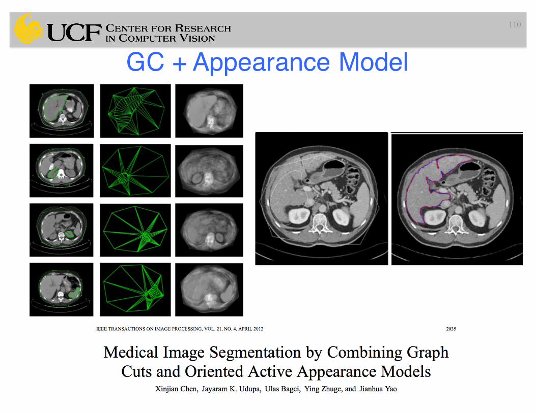
GC + Appearance Model110

GC + Shape Model
111

• Regions used for calculating Dice score, sensitivity, specificity, and robust Hausdorff score. Region T1 is the true lesion area (outline blue), T0 is the remaining normal area. P1 is the area that is predicted to be lesion by—for example—an algorithm (outlined red), and P0 is predicted to be normal. P1 has some overlap with T1 in the right lateral part of the lesion, corresponding to the area referred to as P1Λ T1 in the definition of the Dice score. (Credits: BRATS paper)
112
Summary– Data and Smoothness Terms -> Graph based segmentation methods– Additional terms can(should) be added into segmentation formulation
based observation/need and problem definition– Problems formulated as a MRF task can be solved by max-flow/min-
cut
113

Slide Credits and References• Fredo Durand• M. Tappen• R. Szelisky• http://www.csd.uwo.ca/faculty/yuri/Abstracts/eccv06-tutorial.html• J.Malcolm, Graph Cut in Tensor Scale• Interactive Graph Cuts for Optimal Boundary & Region Segmentation of
Objects in N-D images.Yuri Boykov and Marie-Pierre Jolly.In International Conference on Computer Vision, (ICCV), vol. I, 2001.http://www.csd.uwo.ca/~yuri/Abstracts/iccv01-abs.html
• http://www.cse.yorku.ca/~aaw/Wang/MaxFlowStart.htm• http://research.microsoft.com/vision/cambridge/i3l/segmentation/GrabCut.htm• http://www.cc.gatech.edu/cpl/projects/graphcuttextures/• A Comparative Study of Energy Minimization Methods for Markov Random
Fields. Rick Szeliski, Ramin Zabih, Daniel Scharstein, Olga Veksler, Vladimir Kolmogorov, Aseem Agarwala, Marshall Tappen, Carsten Rother. ECCV 2006www.cs.cornell.edu/~rdz/Papers/SZSVKATR.pdf
• P. Kumar, Oxford University.
114