lecture 11: alternatives to ols with limited dependent ...gasweete/crj604/old/lectures/lecture...
TRANSCRIPT
Lecture 11: Alternatives to OLS with
limited dependent variables, part 2
Poisson
Negative binomial
Tobit
Censored/truncated models
Sample selection corrections

PEA vs APE (again)
PEA: partial effect at the average
The effect of some x on y for a hypothetical case with
sample averages for all x’s.
This is obtained by setting all Xs at their sample
mean and obtaining the slope of Y with respect to
one of the Xs.
APE: average partial effect
The effect of x on y averaged across all cases in the
sample
This is obtained by calculating the partial effect for all
cases, and taking the average.

PEA vs APE: different?
In OLS where the independent variable is
entered in a linear fashion (no squared or
interaction terms), these are equivalent. In fact, it
is an assumption of OLS that the partial effect of
X does not vary across x’s.
PEA and APE differ when we have squared or
interaction terms in OLS, or when we use
logistic, probit, poisson, negative binomial, tobit
or censored regression models.

PEA vs APE in Stata
The “margins” function can report the PEA or the
APE. The PEA may not be very interesting
because, for example, with dichotomous
variables, the average, ranging between 0 and
1, doesn’t correspond to any individuals in our
sample.
. “margins, dydx(x) atmeans” will give you the
PEA for any variable x used in the most
recent regression model.
. “margins, dydx(x)” gives you the APE

PEA vs APE
In regressions with squared or interaction
terms, the margins command will give the
correct answer only if factor variables have
been used
http://www.public.asu.edu/~gasweete/crj604/
misc/factor_variables.pdf

Limited dependent variables
Many problems in criminology require that we analyze
outcomes with very limited distributions
Binary: gang member, arrestee, convict, prisoner
Lots of zeros: delinquency, crime, arrests
Binary & continuous: criminal sentences (prison or
not & sentence length)
Censored: time to re-arrest
We have seen that large-sample OLS can handle
dependent variables with non-normal distributions.
However, sometimes the predictions are nonsensical,
and often they are hetoroskedastic.
Many alternatives to OLS have been developed to deal
with limited dependent variables.

Poisson model
We may use a Poisson model when we have a
dependent variable that takes on only nonnegative
integer values [0,1,2,3, . . .]
We model the relationship between the dependent
an independent variables as follows
1 2 0 1 1( | , ,..., ) exp( ... )k k kE y x x x x x

Poisson model, interpreting
coefficients
Individual coefficients can be interpreted a few different ways. First, we can multiply the coefficient by 100, and interpret it as an expected percent change in Y:
Second, we can exponentiate the coefficient, and interpret the result as the “incident rate ratio” – the factor by which the count is expected to change
% ( | ) (100 )j jE y X x
IRRe j
Poisson model, interpreting
coefficients example
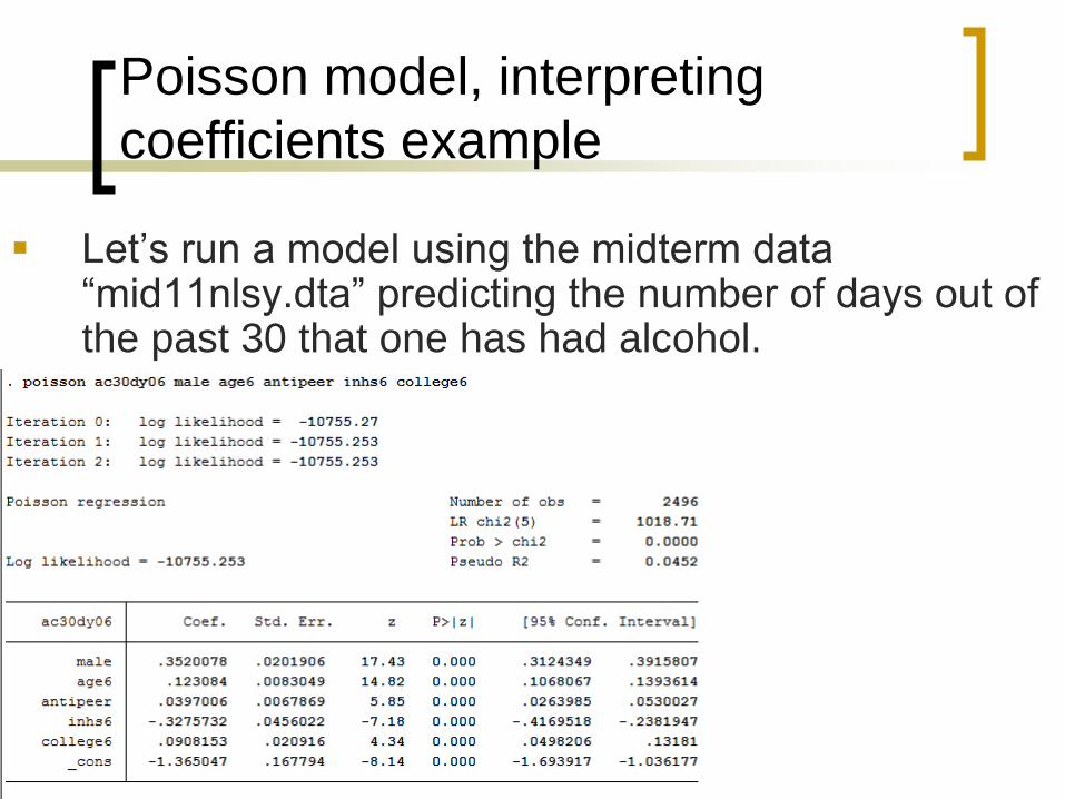
Let’s run a model using the midterm data “mid11nlsy.dta” predicting the number of days out of the past 30 that one has had alcohol.
Poisson model, interpreting
coefficients example
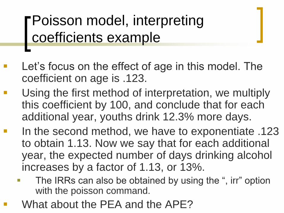
Let’s focus on the effect of age in this model. The coefficient on age is .123.
Using the first method of interpretation, we multiply this coefficient by 100, and conclude that for each additional year, youths drink 12.3% more days.
In the second method, we have to exponentiate .123 to obtain 1.13. Now we say that for each additional year, the expected number of days drinking alcohol increases by a factor of 1.13, or 13%.
The IRRs can also be obtained by using the “, irr” option with the poisson command.
What about the PEA and the APE?

Poisson model, interpreting
coefficients example
The PEA and the APE can be obtained the same way they are obtained after any other regression.
The partial effect at the average is .48. So for the average individual in the sample, an additional year increases the number of days drinking alcohol by .48.
Poisson model, interpreting
coefficients example
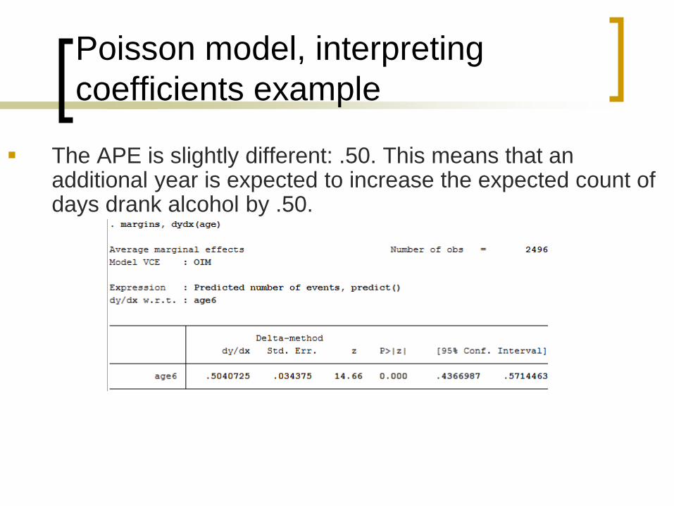
The APE is slightly different: .50. This means that an additional year is expected to increase the expected count of days drank alcohol by .50.

Poisson model, interpreting
coefficients example
How does the average partial effect of .50 square with our initial interpretation that an additional year increases the expected count of days drank alcohol by 12.3 (or 13) percent?
The average days drank alcohol in this sample is 4.09. A 12.3% increase over that would be .50. So the interpretation of the coefficient is the same – one is in percent terms and the other is in terms of actual units in the dependent variable.
When reporting results of Poisson regressions, you may want to report effect sizes in one or more of these days. I find the APE or PEA are the most concrete.
You can also report the partial effect for specific examples:
Poisson model, interpreting
coefficients example
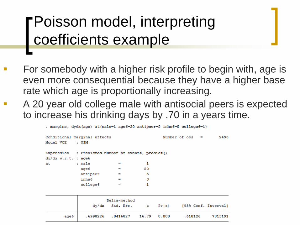
For somebody with a higher risk profile to begin with, age is even more consequential because they have a higher base rate which age is proportionally increasing.
A 20 year old college male with antisocial peers is expected to increase his drinking days by .70 in a years time.
Poisson model, exposure
The standard Poisson model assumes equal “exposure.”
Exposure can be thought of as opportunity or risk. The more
opportunity, the higher the dependent varialbe. In the
example, exposure is 30 days for every person. But it’s not
always the same across units:
Delinquent acts since the last interview, with uneven times between
interviews.
Number of civil lawsuits against corporations. The exposure variable
here would be the number of customers.
Fatal use of force by police departments. Here the exposure variable
would be size of the population served by the police department, or
perhaps number of officers.
The poisson distribution assumes that the variance of Y
equals the mean of Y. This is usually not the case.
Often, we turn to a negative binomial regression instead,
which relaxes the poisson distribution assumption.
Poisson model, exposure
Exposure can be incorporated into the model using the “,
exposure(x)” option where “x” is you variable name for
exposure.
This option inserts logged exposure into the model with a coefficient
fixed to 1. It’s not interpreted, but just adjusts your model so that
exposure is taken into account.
Poisson model, the big
assumption
The poisson distribution assumes that the variance of Y
equals the mean of Y. This is usually not the case.
To test this assumption, we can run “estat gof” which reports
two different goodness-of-fit tests for the Poisson model. If
the p-value is small, our model doesn’t fit well, and we may
need to use a different model.
Often, we turn to a negative binomial regression instead,
which relaxes the poisson distribution assumption.
Negative binomial model example
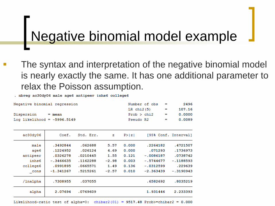
The syntax and interpretation of the negative binomial model
is nearly exactly the same. It has one additional parameter to
relax the Poisson assumption.

Negative binomial model
“Alpha” is the additional parameter, which is used in modeling
dispersion in the dependent variable. If alpha equals zero,
you should just use a Poisson model.
Stata tests the hypothesis that alpha equals zero so that you
can be sure that the negative binomial model is preferable to
the Poisson (when the null hypothesis is rejected).
Another option is a Zero-Inflated Poisson model, which is
essentially a two-part model: a logit model for zero-inflation
and a poisson model for expected count.
We won’t go into this model in detail, but it’s the “zip” command if
you’re interested.
More info here:
http://www.ats.ucla.edu/stat/stata/output/Stata_ZIP.htm

Tobit models
Tobit models are appropriate when the outcome y is
naturally limited in some way. The example in the book is
spending on alcohol. For many people, spending on
alcohol is zero because they don’t consume alcohol, and
for those who do spend money on alcohol, spending
generally follows a normal curve.
There are two processes of interest here: the decision to
spend money on alcohol, and how much money is spent
on alcohol.

Tobit models
The Tobit model assumes that both of these processes
are determined by the relationship between some vector
of Xs and some latent variable y*. Values of y are equal
to y* in some specified range, but below and/or above a
certain threshold, y is equal to the threshold.
Typically, the threshold is zero, but this is not always the
case.
Tobit models,cont.
Several expectations are of interest after estimation of a
Tobit model:
E(y|y>0,x) - expected value of given that y is greater
than zero
E(y|x) – expected value of y
Pr(y>0|x) – probability that y>0 given x
Interestingly, E(y|y>0,x)=E(y|x)*Pr(y>0|x)
Tobit models in Stata, example
17.2
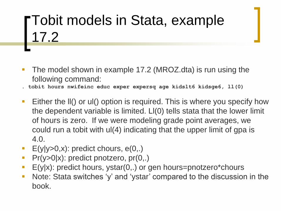
The model shown in example 17.2 (MROZ.dta) is run using the
following command: . tobit hours nwifeinc educ exper expersq age kidslt6 kidsge6, ll(0)
Either the ll() or ul() option is required. This is where you specify how
the dependent variable is limited. Ll(0) tells stata that the lower limit
of hours is zero. If we were modeling grade point averages, we
could run a tobit with ul(4) indicating that the upper limit of gpa is
4.0.
E(y|y>0,x): predict chours, e(0,.)
Pr(y>0|x): predict pnotzero, pr(0,.)
E(y|x): predict hours, ystar(0,.) or gen hours=pnotzero*chours
Note: Stata switches ‘y’ and ‘ystar’ compared to the discussion in the
book.
Tobit models in Stata, example
17.2
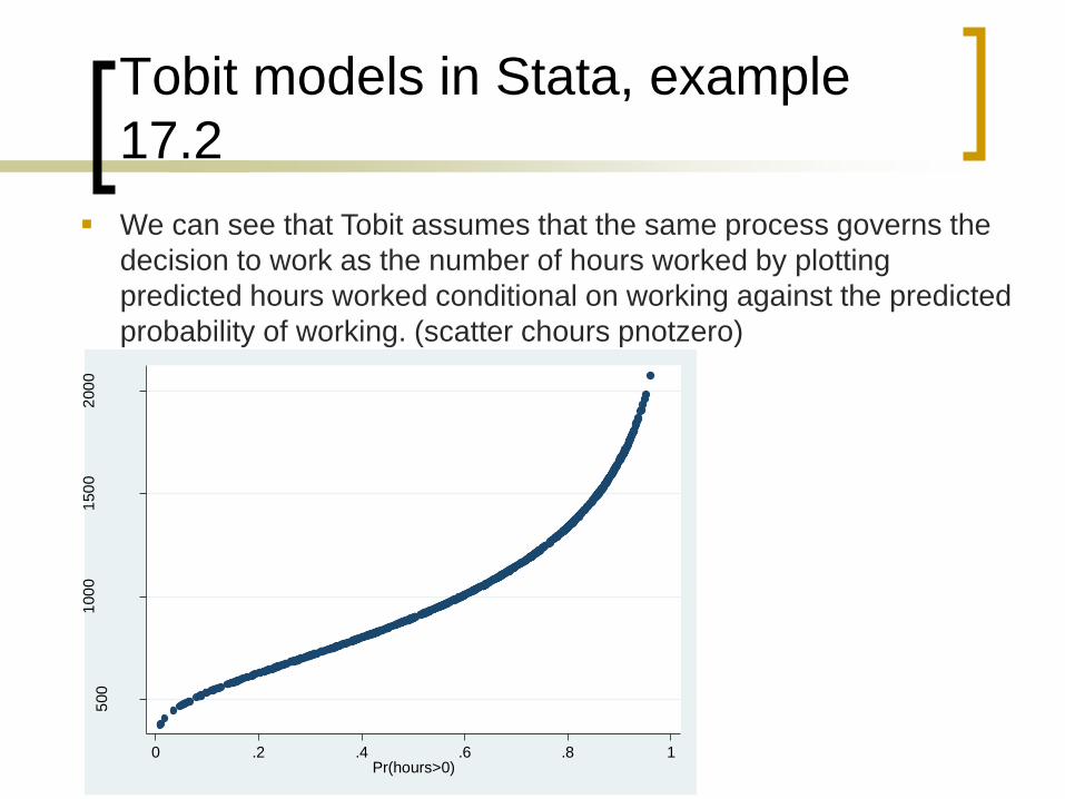
We can see that Tobit assumes that the same process governs the
decision to work as the number of hours worked by plotting
predicted hours worked conditional on working against the predicted
probability of working. (scatter chours pnotzero)
500
100
01
50
02
00
0
E(h
ou
rs|h
ours
>0
)
0 .2 .4 .6 .8 1Pr(hours>0)
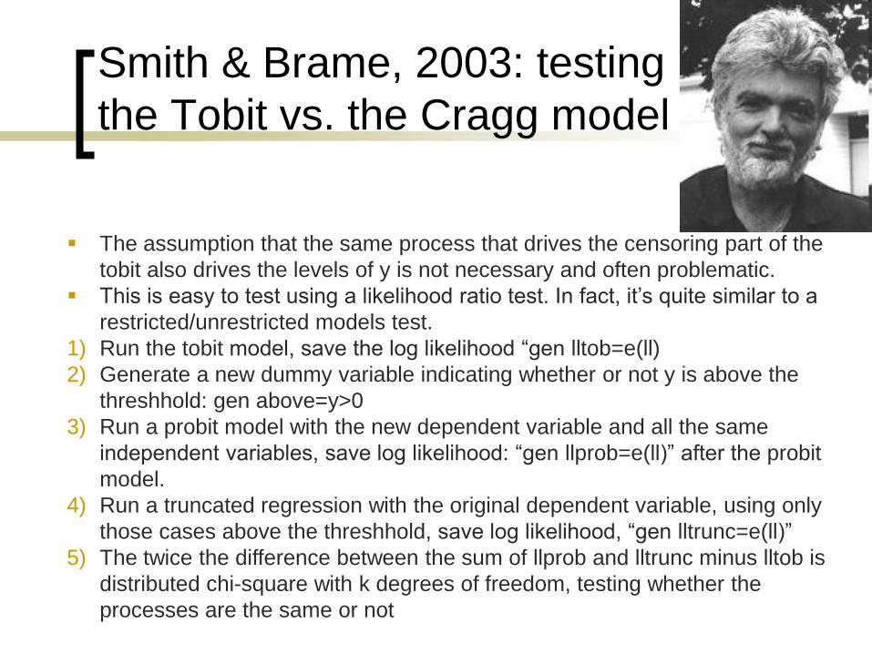
Smith & Brame, 2003: testing
the Tobit vs. the Cragg model
The assumption that the same process that drives the censoring part of the
tobit also drives the levels of y is not necessary and often problematic.
This is easy to test using a likelihood ratio test. In fact, it’s quite similar to a
restricted/unrestricted models test.
1) Run the tobit model, save the log likelihood “gen lltob=e(ll)
2) Generate a new dummy variable indicating whether or not y is above the
threshhold: gen above=y>0
3) Run a probit model with the new dependent variable and all the same
independent variables, save log likelihood: “gen llprob=e(ll)” after the probit
model.
4) Run a truncated regression with the original dependent variable, using only
those cases above the threshhold, save log likelihood, “gen lltrunc=e(ll)”
5) The twice the difference between the sum of llprob and lltrunc minus lltob is
distributed chi-square with k degrees of freedom, testing whether the
processes are the same or not
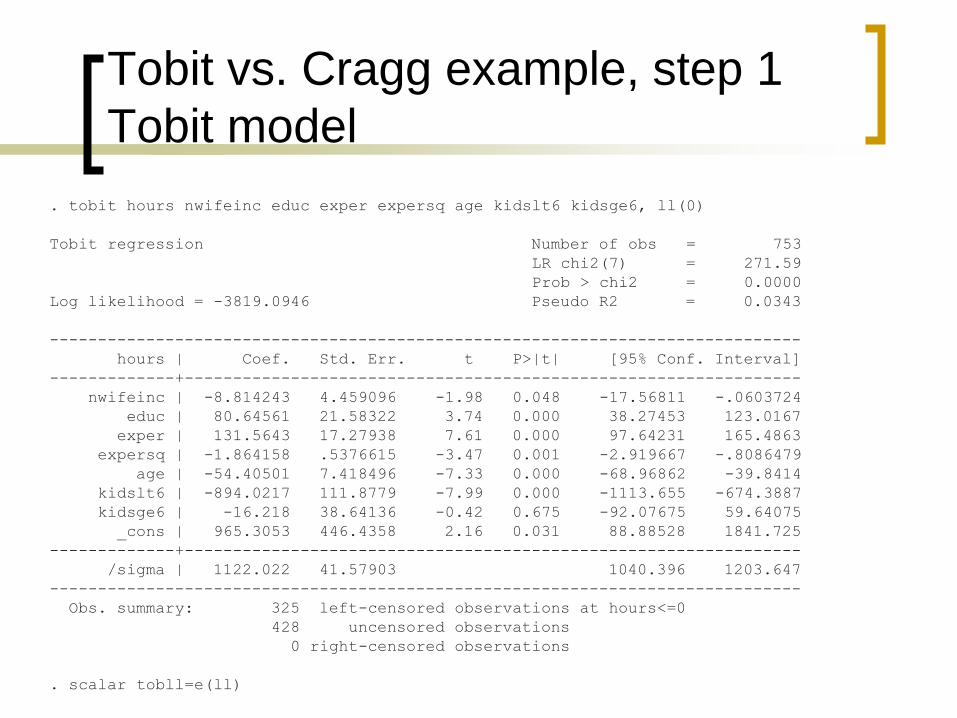
Tobit vs. Cragg example, step 1
Tobit model
. tobit hours nwifeinc educ exper expersq age kidslt6 kidsge6, ll(0)
Tobit regression Number of obs = 753
LR chi2(7) = 271.59
Prob > chi2 = 0.0000
Log likelihood = -3819.0946 Pseudo R2 = 0.0343
------------------------------------------------------------------------------
hours | Coef. Std. Err. t P>|t| [95% Conf. Interval]
-------------+----------------------------------------------------------------
nwifeinc | -8.814243 4.459096 -1.98 0.048 -17.56811 -.0603724
educ | 80.64561 21.58322 3.74 0.000 38.27453 123.0167
exper | 131.5643 17.27938 7.61 0.000 97.64231 165.4863
expersq | -1.864158 .5376615 -3.47 0.001 -2.919667 -.8086479
age | -54.40501 7.418496 -7.33 0.000 -68.96862 -39.8414
kidslt6 | -894.0217 111.8779 -7.99 0.000 -1113.655 -674.3887
kidsge6 | -16.218 38.64136 -0.42 0.675 -92.07675 59.64075
_cons | 965.3053 446.4358 2.16 0.031 88.88528 1841.725
-------------+----------------------------------------------------------------
/sigma | 1122.022 41.57903 1040.396 1203.647
------------------------------------------------------------------------------
Obs. summary: 325 left-censored observations at hours<=0
428 uncensored observations
0 right-censored observations
. scalar tobll=e(ll)
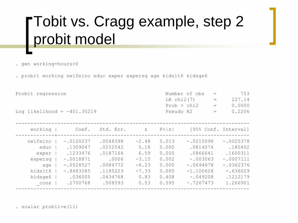
Tobit vs. Cragg example, step 2
probit model
. gen working=hours>0
. probit working nwifeinc educ exper expersq age kidslt6 kidsge6
Probit regression Number of obs = 753
LR chi2(7) = 227.14
Prob > chi2 = 0.0000
Log likelihood = -401.30219 Pseudo R2 = 0.2206
------------------------------------------------------------------------------
working | Coef. Std. Err. z P>|z| [95% Conf. Interval]
-------------+----------------------------------------------------------------
nwifeinc | -.0120237 .0048398 -2.48 0.013 -.0215096 -.0025378
educ | .1309047 .0252542 5.18 0.000 .0814074 .180402
exper | .1233476 .0187164 6.59 0.000 .0866641 .1600311
expersq | -.0018871 .0006 -3.15 0.002 -.003063 -.0007111
age | -.0528527 .0084772 -6.23 0.000 -.0694678 -.0362376
kidslt6 | -.8683285 .1185223 -7.33 0.000 -1.100628 -.636029
kidsge6 | .036005 .0434768 0.83 0.408 -.049208 .1212179
_cons | .2700768 .508593 0.53 0.595 -.7267473 1.266901
------------------------------------------------------------------------------
. scalar probll=e(ll)

Tobit vs. Cragg example, step 3
truncated normal regression
. truncreg hours nwifeinc educ exper expersq age kidslt6 kidsge6, ll(0)
(note: 325 obs. truncated)
Truncated regression
Limit: lower = 0 Number of obs = 428
upper = +inf Wald chi2(7) = 59.05
Log likelihood = -3390.6476 Prob > chi2 = 0.0000
------------------------------------------------------------------------------
hours | Coef. Std. Err. z P>|z| [95% Conf. Interval]
-------------+----------------------------------------------------------------
eq1 |
nwifeinc | .1534399 5.164279 0.03 0.976 -9.968361 10.27524
educ | -29.85254 22.83935 -1.31 0.191 -74.61684 14.91176
exper | 72.62273 21.23628 3.42 0.001 31.00039 114.2451
expersq | -.9439967 .6090283 -1.55 0.121 -2.13767 .2496769
age | -27.44381 8.293458 -3.31 0.001 -43.69869 -11.18893
kidslt6 | -484.7109 153.7881 -3.15 0.002 -786.13 -183.2918
kidsge6 | -102.6574 43.54347 -2.36 0.018 -188.0011 -17.31379
_cons | 2123.516 483.2649 4.39 0.000 1176.334 3070.697
-------------+----------------------------------------------------------------
sigma |
_cons | 850.766 43.80097 19.42 0.000 764.9177 936.6143
------------------------------------------------------------------------------
. scalar truncll=e(ll)
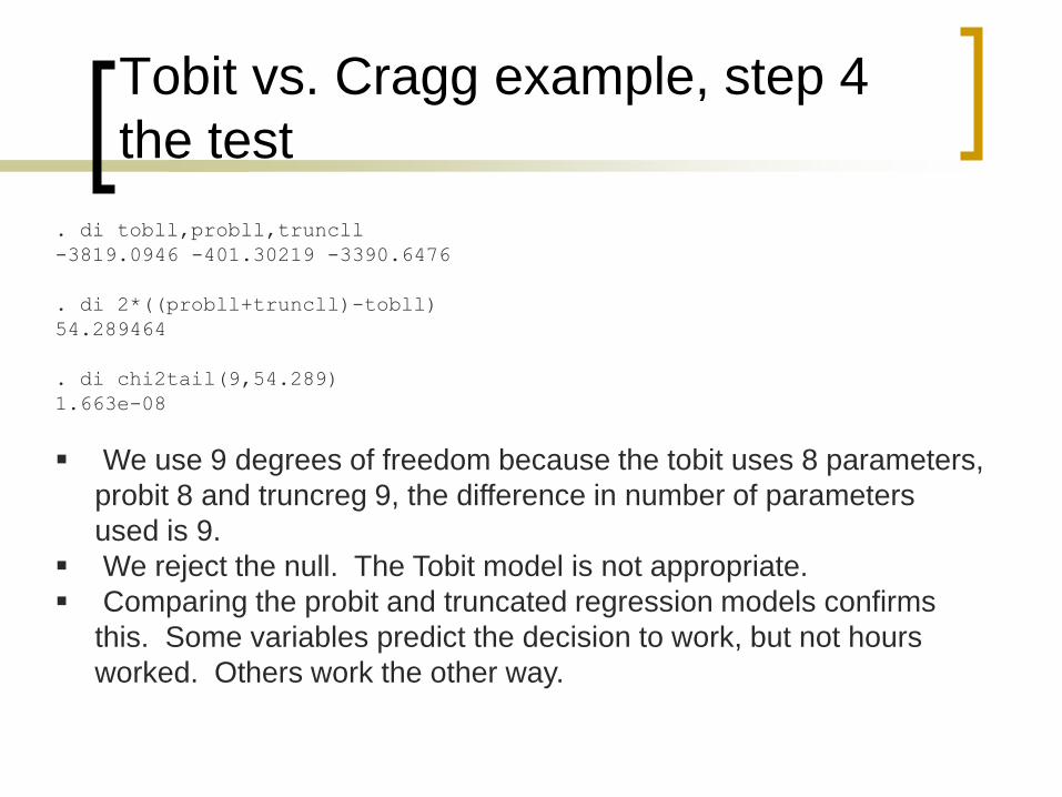
Tobit vs. Cragg example, step 4
the test
. di tobll,probll,truncll
-3819.0946 -401.30219 -3390.6476
. di 2*((probll+truncll)-tobll)
54.289464
. di chi2tail(9,54.289)
1.663e-08
We use 9 degrees of freedom because the tobit uses 8 parameters,
probit 8 and truncreg 9, the difference in number of parameters
used is 9.
We reject the null. The Tobit model is not appropriate.
Comparing the probit and truncated regression models confirms
this. Some variables predict the decision to work, but not hours
worked. Others work the other way.

Censored regression
Use censored regression when the true value of the
dependent variable is unobserved above or below a
certain known threshold.
Censoring is a data collection problem. In the tobit
model, we observe the true values of y, but their
distribution is limited at certain thresholds.
In stata, “cnreg” will give censored regression results.
It requires that you create a new variable with the
values of 0 for uncensored cases, 1 for right
censored cases, and -1 for left censored. If this
variable were called “apple”, for example, you’d write:
“cnreg y x, censored(apple)”

Censored regression
postestimation
The predict function after a censored regression
provides the predicted value of y
The pr(a,b) option for predict gives you the probability
that y falls between the values of a and b.

Truncated regression
Use truncated regression when the sample itself is a
subset of the population of interest. Some cases are
missing entirely.
The truncreg command in Stata will produce truncated
regression estimates
All the same postestimation commands are available
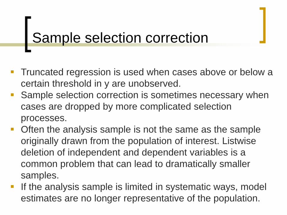
Sample selection correction
Truncated regression is used when cases above or below a
certain threshold in y are unobserved.
Sample selection correction is sometimes necessary when
cases are dropped by more complicated selection
processes.
Often the analysis sample is not the same as the sample
originally drawn from the population of interest. Listwise
deletion of independent and dependent variables is a
common problem that can lead to dramatically smaller
samples.
If the analysis sample is limited in systematic ways, model
estimates are no longer representative of the population.
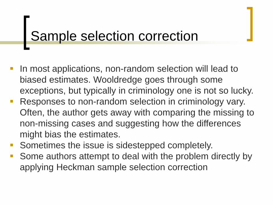
Sample selection correction
In most applications, non-random selection will lead to
biased estimates. Wooldredge goes through some
exceptions, but typically in criminology one is not so lucky.
Responses to non-random selection in criminology vary.
Often, the author gets away with comparing the missing to
non-missing cases and suggesting how the differences
might bias the estimates.
Sometimes the issue is sidestepped completely.
Some authors attempt to deal with the problem directly by
applying Heckman sample selection correction

Sample selection correction
The logic of Heckman’s sample selection correction is that
the selection process is modeled using variables x1 through
xk, and then a correction term is entered in the final
regression along with variables x1 through xj where k≤j
Bushway, Johnson & Slocum (2007) note several problems
with the way the Heckman correction has been applied in
criminology:
1) Use of the logit in the initial step. Probit should be used.
2) Not using OLS in second step.
3) Failure to use exclusion restriction (a variable that
predicts selection but not y)
4) Incorrect calculation of inverse mills ratio

Heckman correction in stata
There are two ways to calculate the Heckman correction in
stata. As noted in the article, the model can be estimated in
a two-step process (probit followed by ols), or all at once
using full-information maximum likelihood (FIML)
estimation.
The two-step method is straightforward, as long as you
calculate the inverse mills ratio correctly
The “heckman” command is the FIML
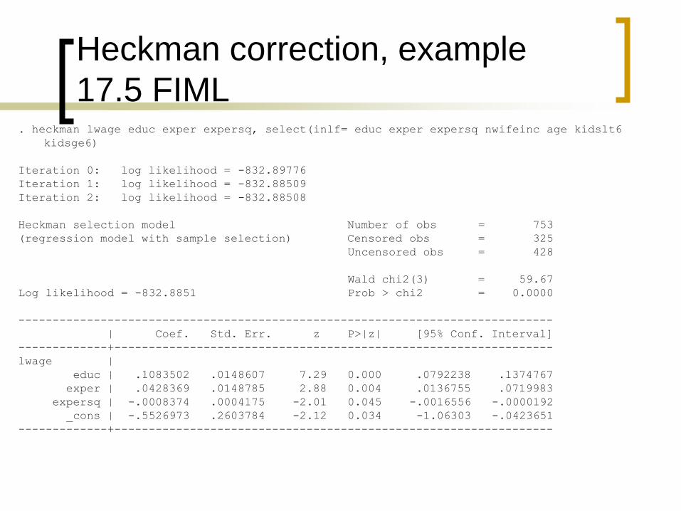
Heckman correction, example
17.5 FIML . heckman lwage educ exper expersq, select(inlf= educ exper expersq nwifeinc age kidslt6
kidsge6)
Iteration 0: log likelihood = -832.89776
Iteration 1: log likelihood = -832.88509
Iteration 2: log likelihood = -832.88508
Heckman selection model Number of obs = 753
(regression model with sample selection) Censored obs = 325
Uncensored obs = 428
Wald chi2(3) = 59.67
Log likelihood = -832.8851 Prob > chi2 = 0.0000
------------------------------------------------------------------------------
| Coef. Std. Err. z P>|z| [95% Conf. Interval]
-------------+----------------------------------------------------------------
lwage |
educ | .1083502 .0148607 7.29 0.000 .0792238 .1374767
exper | .0428369 .0148785 2.88 0.004 .0136755 .0719983
expersq | -.0008374 .0004175 -2.01 0.045 -.0016556 -.0000192
_cons | -.5526973 .2603784 -2.12 0.034 -1.06303 -.0423651
-------------+----------------------------------------------------------------

Heckman correction, example
17.5 FIML cont.
inlf |
educ | .1313415 .0253823 5.17 0.000 .0815931 .1810899
exper | .1232818 .0187242 6.58 0.000 .0865831 .1599806
expersq | -.0018863 .0006004 -3.14 0.002 -.003063 -.0007095
nwifeinc | -.0121321 .0048767 -2.49 0.013 -.0216903 -.002574
age | -.0528287 .0084792 -6.23 0.000 -.0694476 -.0362098
kidslt6 | -.8673988 .1186509 -7.31 0.000 -1.09995 -.6348472
kidsge6 | .0358723 .0434753 0.83 0.409 -.0493377 .1210824
_cons | .2664491 .5089578 0.52 0.601 -.7310898 1.263988
-------------+----------------------------------------------------------------
/athrho | .026614 .147182 0.18 0.857 -.2618573 .3150854
/lnsigma | -.4103809 .0342291 -11.99 0.000 -.4774687 -.3432931
-------------+----------------------------------------------------------------
rho | .0266078 .1470778 -.2560319 .3050564
sigma | .6633975 .0227075 .6203517 .7094303
lambda | .0176515 .0976057 -.1736521 .2089552
------------------------------------------------------------------------------
LR test of indep. eqns. (rho = 0): chi2(1) = 0.03 Prob > chi2 = 0.8577
------------------------------------------------------------------------------
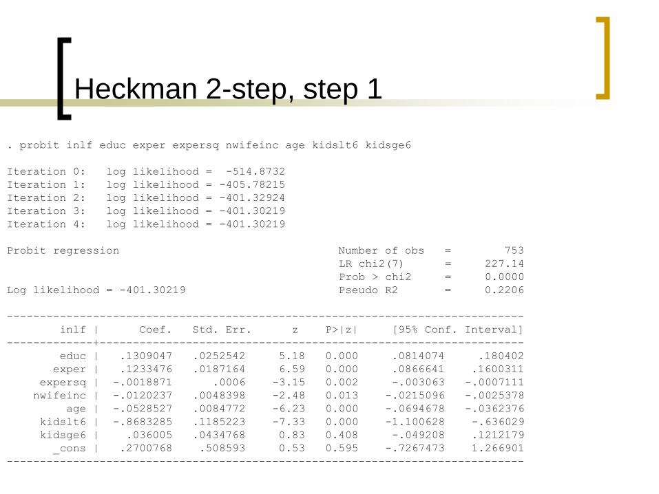
Heckman 2-step, step 1
. probit inlf educ exper expersq nwifeinc age kidslt6 kidsge6
Iteration 0: log likelihood = -514.8732
Iteration 1: log likelihood = -405.78215
Iteration 2: log likelihood = -401.32924
Iteration 3: log likelihood = -401.30219
Iteration 4: log likelihood = -401.30219
Probit regression Number of obs = 753
LR chi2(7) = 227.14
Prob > chi2 = 0.0000
Log likelihood = -401.30219 Pseudo R2 = 0.2206
------------------------------------------------------------------------------
inlf | Coef. Std. Err. z P>|z| [95% Conf. Interval]
-------------+----------------------------------------------------------------
educ | .1309047 .0252542 5.18 0.000 .0814074 .180402
exper | .1233476 .0187164 6.59 0.000 .0866641 .1600311
expersq | -.0018871 .0006 -3.15 0.002 -.003063 -.0007111
nwifeinc | -.0120237 .0048398 -2.48 0.013 -.0215096 -.0025378
age | -.0528527 .0084772 -6.23 0.000 -.0694678 -.0362376
kidslt6 | -.8683285 .1185223 -7.33 0.000 -1.100628 -.636029
kidsge6 | .036005 .0434768 0.83 0.408 -.049208 .1212179
_cons | .2700768 .508593 0.53 0.595 -.7267473 1.266901
------------------------------------------------------------------------------

Heckman 2-step, step 2
. predict xb, xb
. gen imr=normalden(xb)/normal(xb)
. reg lwage educ exper expersq imr
Source | SS df MS Number of obs = 428
-------------+------------------------------ F( 4, 423) = 19.69
Model | 35.0479487 4 8.76198719 Prob > F = 0.0000
Residual | 188.279492 423 .445105182 R-squared = 0.1569
-------------+------------------------------ Adj R-squared = 0.1490
Total | 223.327441 427 .523015084 Root MSE = .66716
------------------------------------------------------------------------------
lwage | Coef. Std. Err. t P>|t| [95% Conf. Interval]
-------------+----------------------------------------------------------------
educ | .1090655 .0156096 6.99 0.000 .0783835 .1397476
exper | .0438873 .0163534 2.68 0.008 .0117434 .0760313
expersq | -.0008591 .0004414 -1.95 0.052 -.0017267 8.49e-06
imr | .0322619 .1343877 0.24 0.810 -.2318889 .2964126
_cons | -.5781032 .306723 -1.88 0.060 -1.180994 .024788
------------------------------------------------------------------------------
General notes
All of these models use maximum likelihood
estimation. Joint hypotheses can be tested with
post-estimation commands as with OLS. Nested
models can be tested using a likelihood ratio test.
Heteroskedasticity and misspecification of these
models can still be a problem and often leads to
worse consequences. Each of these commands
allow for robust variance estimates.

Next time (11/22):
Homework (you have two weeks to do this): 17.6, C17.4
change question ii to “test overdispersion by running a
negative binomial model and reporting the test of
alpha=0, change question iii to “what is the partial effect
at the average for income?” Be sure to use the
appropriate model based on your answer to part ii, and
be sure to include squared income as a factor variable,
C17.6, C17.8 change part ix – don’t use 17.17, just
calculate the APE using the margins command, C17.10
except parts v, vi and vii
Read: Apel & Sweeten (2010)