lecture 11 - interpolation
TRANSCRIPT

Lecture 11Interpolation
T. Gambill
Department of Computer ScienceUniversity of Illinois at Urbana-Champaign
April, 2011
T. Gambill (UIUC) CS 357 April, 2011 1 / 39

Interpolation: Introduction
ObjectiveApproximate an unknown function f (x) by an easier function g(x), such as apolynomial.
Objective (alt)Approximate some data by a function g(x).
Types of approximating functions:1 Polynomials2 Piecewise polynomials3 Rational functions4 Trig functions5 Others (inverse, exponential, Bessel, etc)
T. Gambill (UIUC) CS 357 April, 2011 2 / 39

Basis functionsHow do we approximate a function f (x) by g(x)?
DefinitionWe define the basis functions as a set of functions {φj(x) | j = 0, . . . } and thespace spanned by the basis functions as,
g(x) =n∑
j=0
ajφj(x)
where aj’s can be any real numbers and n is finite.
The function g(x) is said to interpolate the function f (x) at the points(xi, yi) = (xi, f (xi)), i = 0, . . . , n if we can find specific values of aj such that,
g(xi) =
n∑j=0
ajφj(xi) = f (xi) = yi
T. Gambill (UIUC) CS 357 April, 2011 3 / 39

We can solve for the coefficients aj in,
g(xi) =
n∑j=0
ajφj(xi) = f (xi) = yi
by considering the matrix form for the coefficients,φ0(x0) φ1(x0) . . . φn(x0)φ0(x1) φ1(x1) . . . φn(x1)
......
......
φ0(xn) φ1(xn) . . . φn(xn)
∗
a0a1...
an
=
y0y1...
yn
T. Gambill (UIUC) CS 357 April, 2011 4 / 39

MonomialsObvious attempt: try picking the basis functions as φj(x) = xj.
p(x) = a0 + a1x + a2x2 + · · ·+ anxn
So for each xi we have
p(xi) = a0 + a1xi + a2x2i + · · ·+ anxn
i = yi
OR
a0 + a1x0 + a2x20 + · · ·+ anxn
0 = y0
a0 + a1x1 + a2x21 + · · ·+ anxn
1 = y1
a0 + a1x2 + a2x22 + · · ·+ anxn
2 = y2
a0 + a1x3 + a2x23 + · · ·+ anxn
3 = y3
...
a0 + a1xn + a2x2n + · · ·+ anxn
n = yn
T. Gambill (UIUC) CS 357 April, 2011 5 / 39

Monomial: The Vandermonde matrix
so that the matrix form for the coefficients is,1 x0 x2
0 . . . xn0
1 x1 x21 . . . xn
11 x2 x2
2 . . . xn2
...1 xn x2
n . . . xnn
a0a1a2...
an
=
y0y1y2...
yn
QuestionIs this a “good” system to solve?
T. Gambill (UIUC) CS 357 April, 2011 6 / 39
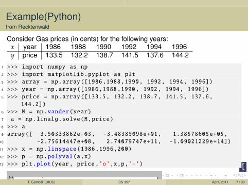
Example(Python)from Recktenwald
Consider Gas prices (in cents) for the following years:x year 1986 1988 1990 1992 1994 1996y price 133.5 132.2 138.7 141.5 137.6 144.2
1 >>> import numpy as np
2 >>> import matplotlib.pyplot as plt
3 >>> array = np.array([1986,1988,1990, 1992, 1994, 1996])
4 >>> year = np.array([1986,1988,1990, 1992, 1994, 1996])
5 >>> price = np.array([133.5, 132.2, 138.7, 141.5, 137.6,
144.2])
6 >>> M = np.vander(year)
7 a = np.linalg.solve(M,price)
8 >>> a
9 array([ 3.50333862e-03, -3.48385098e+01, 1.38578605e+05,
10 -2.75614447e+08, 2.74079747e+11, -1.09021229e+14])
11 >>> x = np.linspace(1986,1996,200)
12 >>> p = np.polyval(a,x)
13 >>> plt.plot(year, price,’o’,x,p,’-’)
T. Gambill (UIUC) CS 357 April, 2011 7 / 39

Example(Python)from Recktenwald
T. Gambill (UIUC) CS 357 April, 2011 8 / 39

Example (MATLAB)from Recktenwald
Consider Gas prices (in cents) for the following years:x year 1986 1988 1990 1992 1994 1996y price 133.5 132.2 138.7 141.5 137.6 144.2
1 year =[1986 1988 1990 1992 1994 1996 ]’;
2
3 price=[133.5 132.2 138.7 141.5 137.6 144.2]’;
4
5 M = vander(year);
6 a = M\price;
7
8 x=linspace(1986,1996,200);
9 p=polyval(a,x);
10 plot(year,price,’o’,x,p,’-’);
T. Gambill (UIUC) CS 357 April, 2011 9 / 39

Interpolation error
In what sense is the approximation a good one?1 Interpolation: g(x) (and/or its derivatives) must have the same values of
f (x) (and/or its derivatives) at set of given points.2 Least-squares: g(x) must deviate as little as possible from f (x) in the
sense of a 2-norm: minimize ||f − g||22 =∫b
a |f (t) − g(t)|2 dt3 Chebyshev: g(x) must deviate as little as possible from f (x) in the sense
of the ∞-norm: minimize maxt∈[a,b] |f (t) − g(t)|.
T. Gambill (UIUC) CS 357 April, 2011 10 / 39

Interpolating polynomial is unique!
Given n + 1 distinct points x0, . . . , xn, and values y0, . . . , yn, find a polynomialp(x) of degree at most n so that
p(xi) = yi i = 0, . . . , n
A polynomial of degree n has n + 1 degrees-of-freedom:
p(x) = a0 + a1x + · · ·+ anxn
n + 1 constraints determine the polynomial uniquely:
p(xi) = yi, i = 0, . . . , n
TheoremIf points x0, . . . , xn are distinct, then for arbitrary y0, . . . , yn, there is a uniquepolynomial p(x) of degree at most n such that p(xi) = yi for i = 0, . . . , n. Thisunique polynomial is the minimal degree polynomial where p(xi) = yi fori = 0, . . . , n.
T. Gambill (UIUC) CS 357 April, 2011 11 / 39

Fundamental Theorem of Algebra
How can you prove the interpolating polynomial is unique, so that we canspeak of the interpolating polynomial? Assume that it isn’t, then apply thefollowing form of the Fundamental Theorem of Algebra.
TheoremEvery non-zero polynomial has exactly as many complex roots as its degree,where each root is counted up to its multiplicity.
T. Gambill (UIUC) CS 357 April, 2011 12 / 39

Interpolation error using the unique interpolatingpolynomial
TheoremGiven function f with n + 1 continuous derivatives in the interval formed by I =[min({x, x0, . . . , xn}), max({x, x0, . . . , xn})]. If p(x) is the unique interpolatingpolynomial of degree 6 n with,
p(xi) = f (xi), i = 0, 1, . . . , n
then the error is computed by the formula,
p(x) − f (x) =f (n+1)(ξ(x))(n + 1)!
(x − x0)(x − x1) . . . (x − xn), for some ξ(x) ∈ I
T. Gambill (UIUC) CS 357 April, 2011 13 / 39

Interpolating Runge’s functionIf we interpolate Runge’s function,
f (x) =1
1 + 25x2
on the interval [−1, 1] with equally spaced points we get the following results:
Higher degree interpolating polynomials can be problematic.T. Gambill (UIUC) CS 357 April, 2011 14 / 39

1 function runge()
2 close all
3 % plot runge’s function
4 x2 = linspace(-1,1,200);
5 y2 = 1./(1+25*x2.ˆ2);
6 plot(x2,y2);
7 hold all
8 % plot using interp polys
9 for i = [5 7 11]
10 x = linspace(-1,1,i);
11 y = 1./(1+25*x.ˆ2);
12 p = polyfit(x,y,i-1);
13 %
14 x2 = linspace(-1,1,200);
15 y2 = polyval(p,x2);
16 plot(x2,y2);
17 pause
18 end
19 legend(’runge’,’4’, ’6’, ’10’)
T. Gambill (UIUC) CS 357 April, 2011 15 / 39

Monomial Basis
The Matlab function polyfit uses QR factorization to compute the coefficientsfor the interpolating polynomial, with a cost of O(n3) for an n-th degreepolynomial. To evaluate the interpolating polynomial we can use Horner’smethod which has a cost of O(n).
Horner’s methodThe polynomial
p(x) = a0 + a1x + a2x2 + · · ·+ an−1xn−1 + anxn
can be efficiently computed as,
p(x) = a0 + x(a1 + x(a2 + · · ·+ x(an−1 + anx) . . . ))
T. Gambill (UIUC) CS 357 April, 2011 16 / 39

Polynomial Interpolation Strategy
Lower Degree PolynomialInterpolation
Use piecewise polynomials (Splines)
Higher Degree PolynomialInterpolation
Use non-uniform spacing (Chebyshev)Use basis functions that yieldcoefficients that are easier to compute(Lagrange or Newton)
T. Gambill (UIUC) CS 357 April, 2011 17 / 39

Chebyshev NodesChebyshev nodes in [−1, 1]
xi = cos((
2i + 12
)π
n + 1
), i = 0, . . . , n
Can obtain nodes from equidistant points on a circle projected downNodes are non uniform and non nested
T. Gambill (UIUC) CS 357 April, 2011 18 / 39
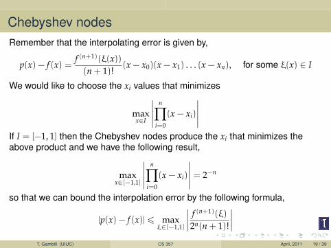
Chebyshev nodesRemember that the interpolating error is given by,
p(x) − f (x) =f (n+1)(ξ(x))(n + 1)!
(x − x0)(x − x1) . . . (x − xn), for some ξ(x) ∈ I
We would like to choose the xi values that minimizes
maxx∈I
∣∣∣∣∣n∏
i=0
(x − xi)
∣∣∣∣∣If I = [−1, 1] then the Chebyshev nodes produce the xi that minimizes theabove product and we have the following result,
maxx∈[−1,1]
∣∣∣∣∣n∏
i=0
(x − xi)
∣∣∣∣∣ = 2−n
so that we can bound the interpolation error by the following formula,
|p(x) − f (x)| 6 maxξ∈[−1,1]
∣∣∣∣ f (n+1)(ξ)
2n(n + 1)!
∣∣∣∣T. Gambill (UIUC) CS 357 April, 2011 19 / 39

Lagrange polynomials
The general form for the Lagrange basis functions is
`k(x) =n∏
i=0,i,k
x − xi
xk − xi
The resulting interpolating polynomial is
p(x) =n∑
k=0
yk`k(x)
so the matrix form for the coefficients is,y0y1...
yn
=
`0(x0) `1(x0) . . . `n(x0)`0(x1) `1(x1) . . . `n(x1)
......
......
`0(xn) `1(xn) . . . `n(xn)
∗
a0a1...
an
=
1 0 . . . 00 1 . . . 0...
......
...0 0 . . . 1
∗
a0a1...
an
T. Gambill (UIUC) CS 357 April, 2011 20 / 39

Back to the basics...
ExampleFind the interpolating polynomial of least degree that interpolates
x 1.4 1.25y 3.7 3.9
Directly
p1(x) =(
x − 1.251.4 − 1.25
)3.7 +
(x − 1.4
1.25 − 1.4
)3.9
= 3.7 +
(3.9 − 3.7
1.25 − 1.4
)(x − 1.4)
= 3.7 −43(x − 1.4)
T. Gambill (UIUC) CS 357 April, 2011 21 / 39
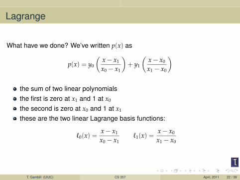
Lagrange
What have we done? We’ve written p(x) as
p(x) = y0
(x − x1
x0 − x1
)+ y1
(x − x0
x1 − x0
)
the sum of two linear polynomialsthe first is zero at x1 and 1 at x0
the second is zero at x0 and 1 at x1
these are the two linear Lagrange basis functions:
`0(x) =x − x1
x0 − x1`1(x) =
x − x0
x1 − x0
T. Gambill (UIUC) CS 357 April, 2011 22 / 39

Lagrange
ExampleWrite the Lagrange basis functions for
x 13
14 1
y 2 -1 7
Directly
`0(x) =(x − 1
4 )(x − 1)( 1
3 − 14 )(
13 − 1)
`1(x) =(x − 1
3 )(x − 1)( 1
4 − 13 )(
14 − 1)
`2(x) =(x − 1
3 )(x − 14 )
(1 − 13 )(1 − 1
4 )
T. Gambill (UIUC) CS 357 April, 2011 23 / 39

ExampleFind the equation of the parabola passing through the points (1,6), (-1,0), and(2,12)
x0 = 1, x1 = −1, x2 = 2; y0 = 6, y1 = 0, y2 = 12;
`0(x) = (x−x1)(x−x2)(x0−x1)(x0−x2)
= (x+1)(x−2)(2)(−1)
`1(x) = (x−x0)(x−x2)(x1−x0)(x1−x2)
= (x−1)(x−2)(−2)(−3)
`2(x) = (x−x0)(x−x1)(x2−x0)(x2−x1)
= (x−1)(x+1)(1)(3)
p2(x) = y0`0(x) + y1`1(x) + y2`2(x)
= −3× (x + 1)(x − 2) + 0× 16(x − 1)(x − 2)
+4× (x − 1)(x + 1)= (x + 1)[4(x − 1) − 3(x − 2)]= (x + 1)(x + 2)
T. Gambill (UIUC) CS 357 April, 2011 24 / 39
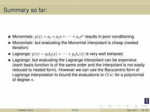
Summary so far:
Monomials: p(x) = a0 + a1x + · · ·+ anxn results in poor conditioningMonomials: but evaluating the Monomial interpolant is cheap (nestediteration)Lagrange: p(x) = y0`0(x) + · · ·+ yn`n(x) is very well behaved.Lagrange: but evaluating the Lagrange interpolant can be expensive(each basis function is of the same order and the interpolant is not easilyreduced to nested form). However we can use the Barycentric form ofLagrange interpolation to bound the evaluations to O(n) for a polynomialof degree n.
T. Gambill (UIUC) CS 357 April, 2011 25 / 39

Improving evaluation of Lagrange polynomialsIf we denote,
`(x) = (x − x0)(x − x1) . . . (x − xn)
then we can write the Lagrange basis functions as,
`k(x) =`(x)
(x − xk)
1∏ni=0,i,k(xk − xi)
and thus if we compute,
wk =1∏n
i=0,i,k(xk − xi)
we can write the Lagrange interpolating polynomial as,
p(x) = `(x)n∑
k=0
wk
x − xkyk
If we pre-compute and store the wk (for a cost of O(n2)) then computing p(x) isreduced to a cost of O(n).
T. Gambill (UIUC) CS 357 April, 2011 26 / 39

Newton Polynomials
Newton Polynomials are of the form
pn(x) = a0 + a1(x− x0) + a2(x− x0)(x− x1) + a3(x− x0)(x− x1)(x− x2) + . . .
The basis used is thusfunction order1 0x − x0 1(x − x0)(x − x1) 2(x − x0)(x − x1)(x − x2) 3
More stable than monomialsAs computationally efficient (nested iteration) as Barycentric Lagrangeinterpolation
T. Gambill (UIUC) CS 357 April, 2011 27 / 39

Newton Polynomials using Divided Differences
Consider the data
x0 x1 x2
y0 y1 y2
We want to find a0, a1, and a2 in the following polynomial so that it fits the data:
p2(x) = a0 + a1(x − x0) + a2(x − x0)(x − x1)
Matching the data gives three equations to determine our three unknowns ai:
at x0: y0 = a0 + 0 + 0at x1: y1 = a0 + a1(x1 − x0) + 0at x2: y2 = a0 + a1(x2 − x0) + a2(x2 − x0)(x2 − x1)
T. Gambill (UIUC) CS 357 April, 2011 28 / 39
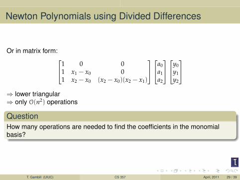
Newton Polynomials using Divided Differences
Or in matrix form:1 0 01 x1 − x0 01 x2 − x0 (x2 − x0)(x2 − x1)
a0a1a2
y0y1y2
⇒ lower triangular⇒ only O(n2) operations
QuestionHow many operations are needed to find the coefficients in the monomialbasis?
T. Gambill (UIUC) CS 357 April, 2011 29 / 39

Newton Polynomials using Divided Differences
Using Forward Substitution to solve this lower triangular system yields:
a0 = y0 = f (x0)
a1 =y1 − a0
x1 − x0
=f (x1) − f (x0)
x1 − x0
a2 =y2 − a0 − (x2 − x0)a1
(x2 − x1)(x2 − x0)
= ... next slide
T. Gambill (UIUC) CS 357 April, 2011 30 / 39

Newton Polynomials using Divided Differences
From the previous slide . . .
a2 =f (x2) − f (x0) − (x2 − x0)
f(x1)−f(x0)x1−x0
(x2 − x1)(x2 − x0)
=f (x2) − f (x1) + f (x1) − f (x0) − (x2 − x0)
f(x1)−f(x0)x1−x0
(x2 − x1)(x2 − x0)
=f (x2) − f (x1) + (f (x1) − f (x0))
(1 − x2−x0
x1−x0
)(x2 − x1)(x2 − x0)
=f (x2) − f (x1) + (f (x1) − f (x0))
(x1−x2x1−x0
)(x2 − x1)(x2 − x0)
=
f(x2)−f(x1)x2−x1
−f(x1)−f(x0)
x1−x0
x2 − x0
T. Gambill (UIUC) CS 357 April, 2011 31 / 39

Newton Polynomials using Divided DifferencesFrom this we see a pattern. There are many terms of the form
f (xj) − f (xi)
xj − xi
These are called divided differences and are denoted with square brackets:
f [xi, xj] =f (xj) − f (xi)
xj − xi
Applying this to our results:
a0 = f [x0]
a1 = f [x0, x1]
a2 =f [x1, x2] − f [x0, x1]
x2 − x0
= f [x0, x1, x2]
T. Gambill (UIUC) CS 357 April, 2011 32 / 39

Newton Polynomials using Divided Differences
We can now write the interpolating polynomial as,
p(x) = f [x0]+f [x0, x1](x−x0)+f [x0, x1, x2](x−x0)(x−x1)+· · ·+f [x0, . . . , xn](x−x0) . . . (x−xn−1)
T. Gambill (UIUC) CS 357 April, 2011 33 / 39

Newton Polynomials using Divided Differencesexample: long way
ExampleFor the data
x 1 -4 0y 3 13 -23
Find the 2nd order interpolating polynomial using Newton.
We knowp2(x) = a0 + a1(x − x0) + a2(x − x0)(x − x1)
And that
a0 = f [x0] = f [1] = f (1) = 3
a1 = f [x0, x1] =f (x1) − f (x0)
x1 − x0=
13 − 3−4 − 1
= −2
a2 = f [x0, x1, x2] =f [x1, x2] − f [x0, x1]
x2 − x0
=−23−13
0−−4 − 13−3−4−1
0 − 1
=−9 + 2−1
= 7
Sop2(x) = 3 − 2(x − 1) + 7(x − 1)(x + 4)
T. Gambill (UIUC) CS 357 April, 2011 34 / 39

Divided Differences
Recursive Property
f [x0, . . . , xk] =f [x1, . . . , xk] − f [x0, . . . , xk−1]
xk − x0
With the first two defined by
f [xi] = f (xi)
f [xi, xj] =f [xj] − f [xi]
xj − xi
T. Gambill (UIUC) CS 357 April, 2011 35 / 39
Divided Differences
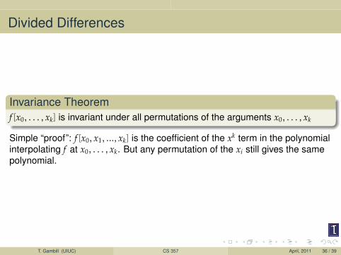
Invariance Theoremf [x0, . . . , xk] is invariant under all permutations of the arguments x0, . . . , xk
Simple “proof”: f [x0, x1, ..., xk] is the coefficient of the xk term in the polynomialinterpolating f at x0, . . . , xk. But any permutation of the xi still gives the samepolynomial.
T. Gambill (UIUC) CS 357 April, 2011 36 / 39

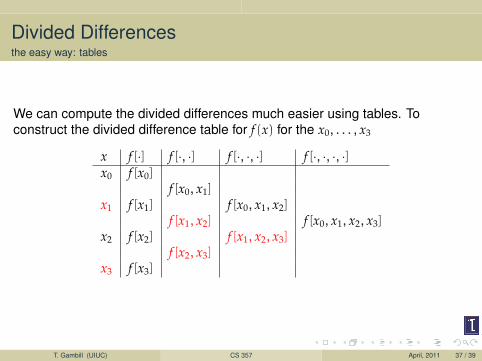
Divided Differencesthe easy way: tables
We can compute the divided differences much easier using tables. Toconstruct the divided difference table for f (x) for the x0, . . . , x3
x f [·] f [·, ·] f [·, ·, ·] f [·, ·, ·, ·]x0 f [x0]
f [x0, x1]x1 f [x1] f [x0, x1, x2]
f [x1, x2] f [x0, x1, x2, x3]x2 f [x2] f [x1, x2, x3]
f [x2, x3]x3 f [x3]
T. Gambill (UIUC) CS 357 April, 2011 37 / 39
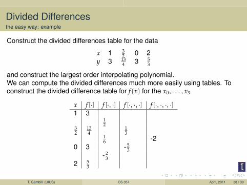
Divided Differencesthe easy way: example
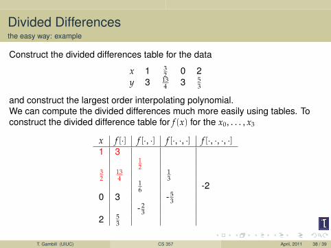
Construct the divided differences table for the data
x 1 32 0 2
y 3 134 3 5
3
and construct the largest order interpolating polynomial.We can compute the divided differences much more easily using tables. Toconstruct the divided difference table for f (x) for the x0, . . . , x3
x f [·] f [·, ·] f [·, ·, ·] f [·, ·, ·, ·]1 3
12
32
134
13
16 -2
0 3 - 53
- 23
2 53
T. Gambill (UIUC) CS 357 April, 2011 38 / 39
Divided Differencesthe easy way: example
Construct the divided differences table for the data
x 1 32 0 2
y 3 134 3 5
3
and construct the largest order interpolating polynomial.We can compute the divided differences much more easily using tables. Toconstruct the divided difference table for f (x) for the x0, . . . , x3
x f [·] f [·, ·] f [·, ·, ·] f [·, ·, ·, ·]1 3
12
32
134
13
16 -2
0 3 - 53
- 23
2 53
T. Gambill (UIUC) CS 357 April, 2011 38 / 39

Divided Differencesthe easy way: example
x f [·] f [·, ·] f [·, ·, ·] f [·, ·, ·, ·]1 3
12
32
134
13
16 -2
0 3 - 53
- 23
2 53
The coefficients are readily available and we arrive at
p3(x) = 3 +12(x − 1) +
13(x − 1)(x −
32) − 2(x − 1)(x −
32)x
T. Gambill (UIUC) CS 357 April, 2011 39 / 39