Lecture 22Lecture 22

NumericalAnalysis

NumericalAnalysis

Chapter 5Interpolation

Chapter 5Interpolation

Finite Difference OperatorsFinite Difference OperatorsNewton’s Forward Difference Newton’s Forward Difference Interpolation FormulaInterpolation FormulaNewton’s Backward Difference Newton’s Backward Difference

Interpolation FormulaInterpolation FormulaLagrange’s Interpolation Lagrange’s Interpolation FormulaFormulaDivided DifferencesDivided DifferencesInterpolation in Two DimensionsInterpolation in Two DimensionsCubic Spline InterpolationCubic Spline Interpolation

Finite Difference OperatorsFinite Difference OperatorsNewton’s Forward Difference Newton’s Forward Difference Interpolation FormulaInterpolation FormulaNewton’s Backward Difference Newton’s Backward Difference

Interpolation FormulaInterpolation FormulaLagrange’s Interpolation Lagrange’s Interpolation FormulaFormulaDivided DifferencesDivided DifferencesInterpolation in Two DimensionsInterpolation in Two DimensionsCubic Spline InterpolationCubic Spline Interpolation

1 11

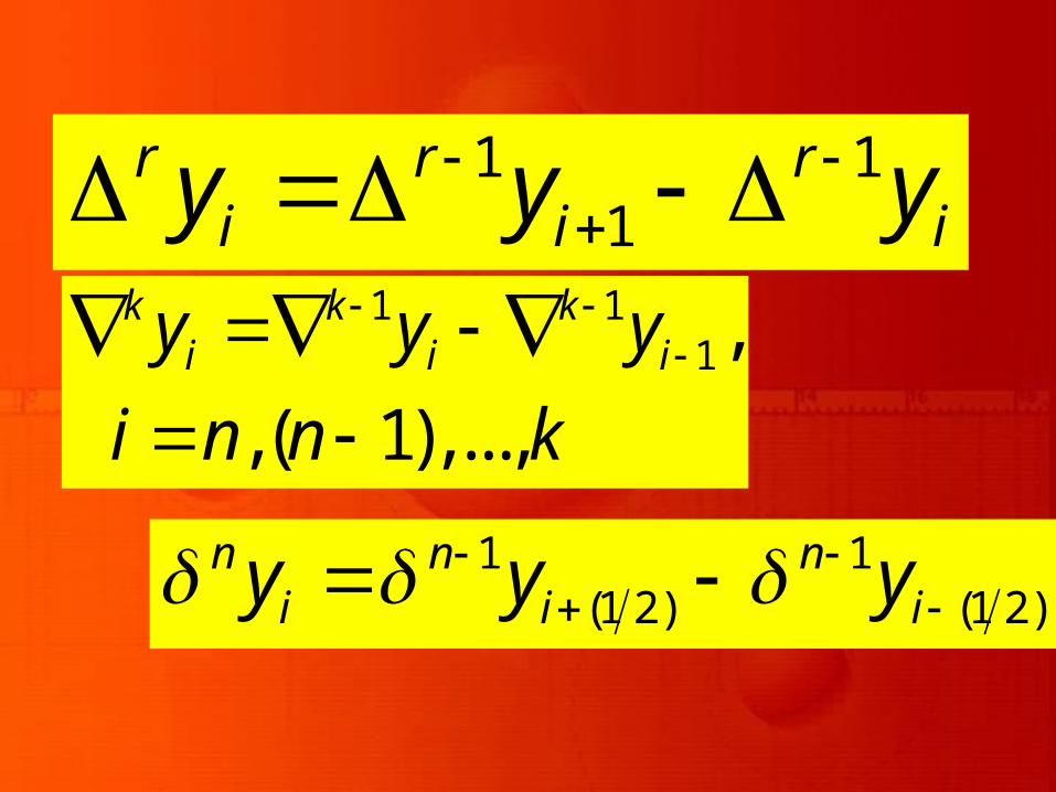
r r ri i iy y y

1 1

1,

, ( 1),...,

k k ki i iy y y

i n n k

1 1

(1 2) (1 2)n n ni i iy y y

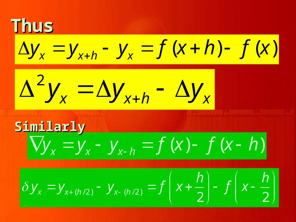
ThusThus( ) ( )x x h xy y y f x h f x

2x x h xy y y

( ) ( )x x x hy y y f x f x h

( / 2) ( / 2) 2 2x x h x h

h hy y y f x f x

SimilarlySimilarly

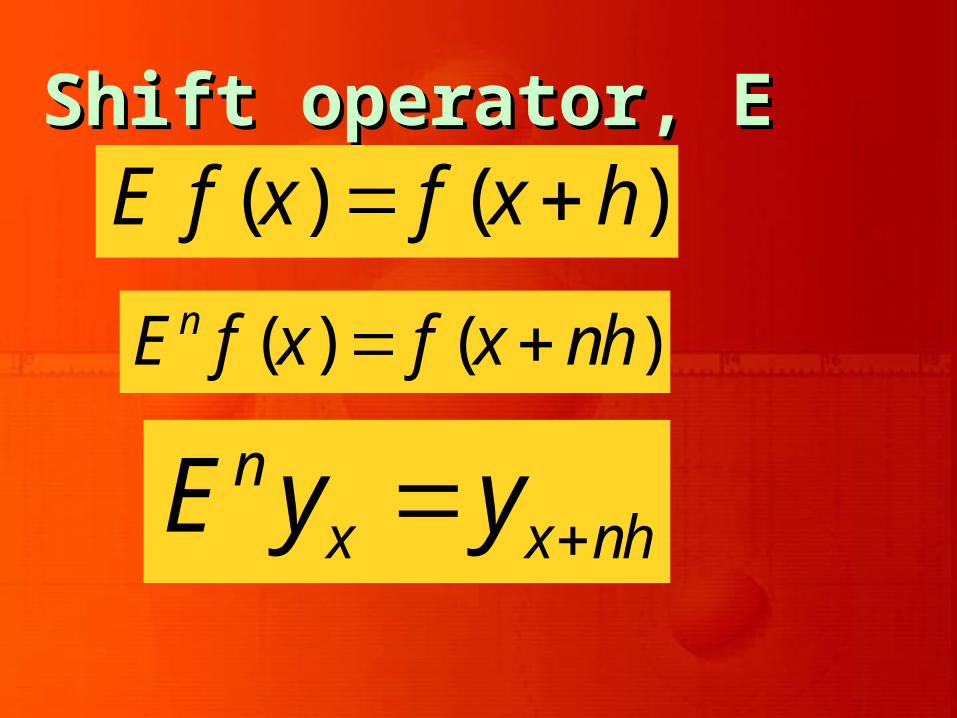
Shift operator, EShift operator, E( ) ( )E f x f x h

( ) ( )nE f x f x nh

nx x nhE y y

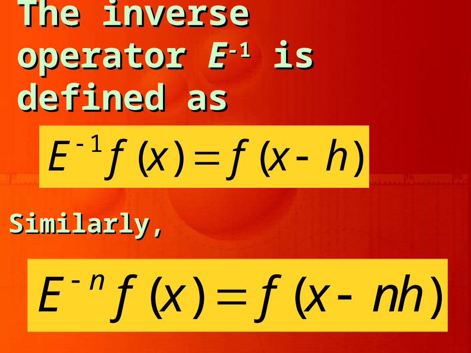
The inverse operator The inverse operator EE-1-1 is defined asis defined as

1 ( ) ( )E f x f x h Similarly,Similarly,

( ) ( )nE f x f x nh

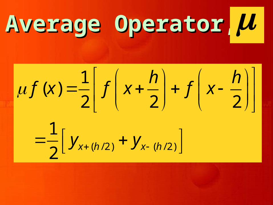
Average Operator, Average Operator,

( / 2) ( / 2)

1( )

2 2 2

1

2 x h x h

h hf x f x f x

y y

22

2

( ) ( ) ( )

( ) ( ) ( )n

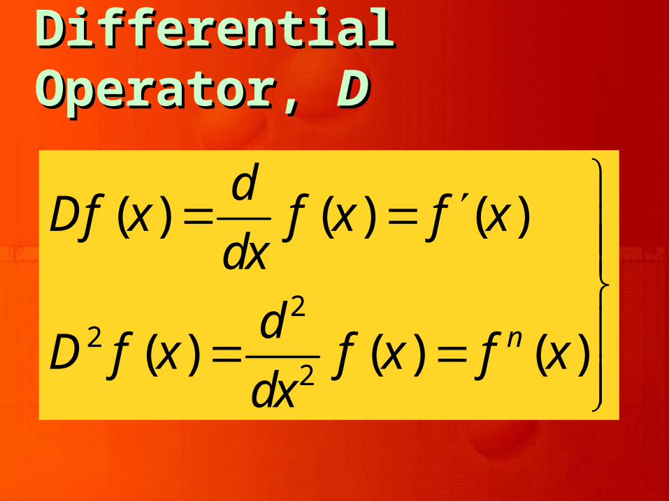
dDf x f x f x

dx

dD f x f x f x

dx

Differential Operator, Differential Operator, DD

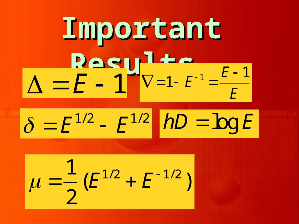
Important Results Important Results 1E 1 1

1E

EE

1/ 2 1/ 2E E

1/ 2 1/ 21( )

2E E

loghD E

Newton’s Forward

Difference Interpolation

Formula

Newton’s Forward

Difference Interpolation

Formula

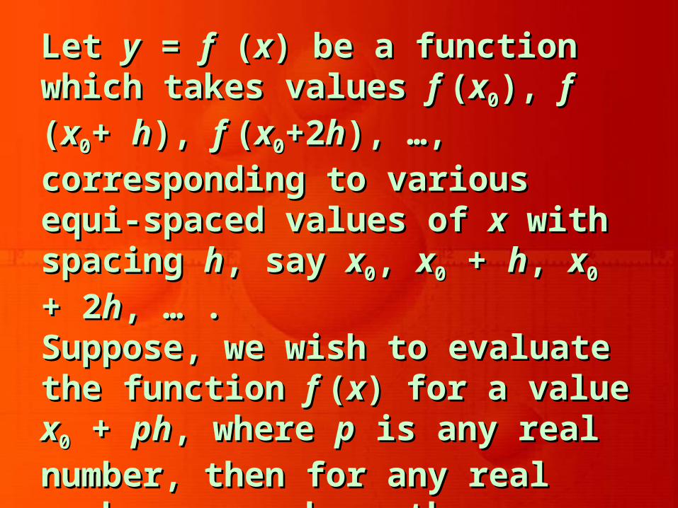
Let Let yy = = ff ( (xx) be a function which ) be a function which takes values takes values f f ((xx00), ), f f ((xx00+ + hh), ), f f ((xx00+2+2hh), ),

…, corresponding to various equi-…, corresponding to various equi-spaced values of spaced values of xx with spacing with spacing hh, , say say xx00, , xx00 + + hh, , xx00 + 2 + 2hh, … . , … .

Suppose, we wish to evaluate the Suppose, we wish to evaluate the function function f f ((xx) for a value ) for a value xx00 + + phph, ,

where where pp is any real number, then for is any real number, then for any real number any real number pp, we have the , we have the operator operator EE such that such that

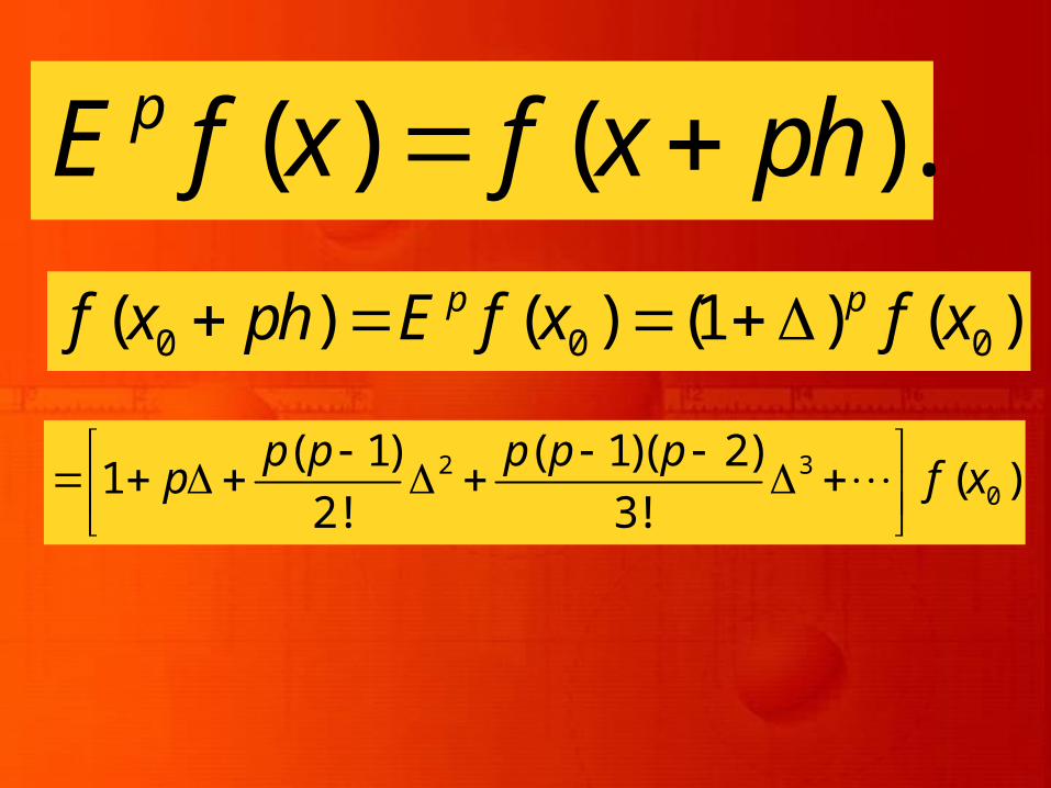
( ) ( ).pE f x f x ph

0 0 0( ) ( ) (1 ) ( )p pf x ph E f x f x

2 30

( 1) ( 1)( 2)1 ( )

2! 3!

p p p p pp f x

0 0 0

2 30 0

0

( ) ( ) ( )

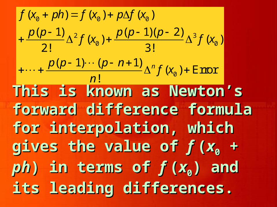
( 1) ( 1)( 2)( ) ( )

2! 3!( 1) ( 1)

( ) Error!

n

f x ph f x p f x

p p p p pf x f x

p p p nf x

n

This is known as Newton’s This is known as Newton’s forward difference formula for forward difference formula for interpolation, which gives the interpolation, which gives the value of value of f f ((xx00 + + phph) in terms of ) in terms of f f ((xx00) )

and its leading differences. and its leading differences.

20 0 0

30

0

( 1)

2!( 1)( 2)

3!( 1)( 1)

Error!

x

n

p py y p y y

p p py

p p p ny

n

This formula is also known as This formula is also known as Newton-Gregory forward Newton-Gregory forward difference interpolation formula. difference interpolation formula. Here p=(x-xHere p=(x-x00)/h.)/h.

An alternate expression isAn alternate expression is

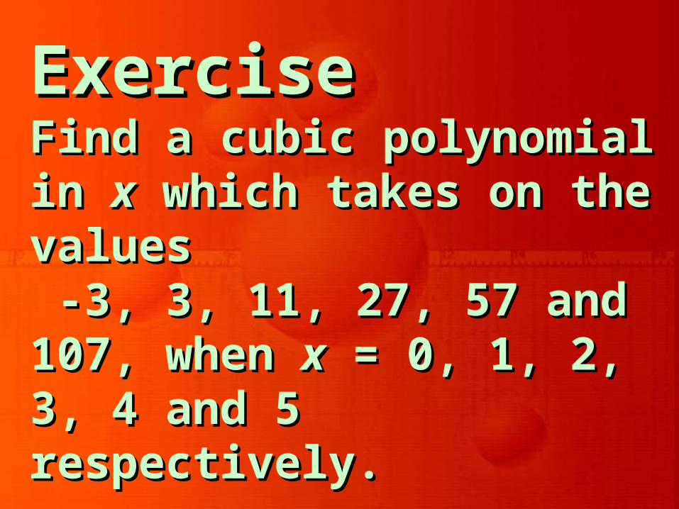
Exercise Exercise Find a cubic polynomial in Find a cubic polynomial in xx which takes on the valueswhich takes on the values -3, 3, 11, 27, 57 and 107, -3, 3, 11, 27, 57 and 107, when when xx = 0, 1, 2, 3, 4 and 5 = 0, 1, 2, 3, 4 and 5 respectively.respectively.

SolutionSolution Here, the observations are Here, the observations are given at equal intervals of unit given at equal intervals of unit width.width.To determine the required To determine the required polynomial, we first construct polynomial, we first construct the difference table the difference table

Difference TableDifference Table

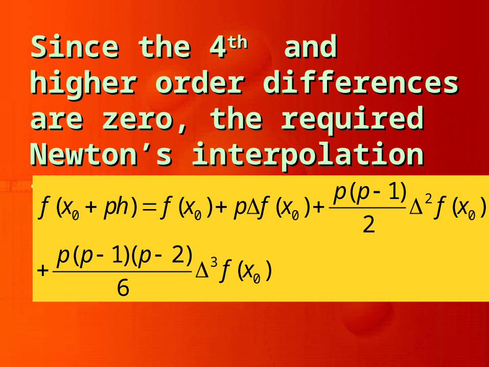
Since the 4Since the 4thth and higher order and higher order differences are zero, the differences are zero, the required Newton’s required Newton’s interpolation formulainterpolation formula

20 0 0 0

30

( 1)( ) ( ) ( ) ( )

2( 1)( 2)

( )6

p pf x ph f x p f x f x

p p pf x

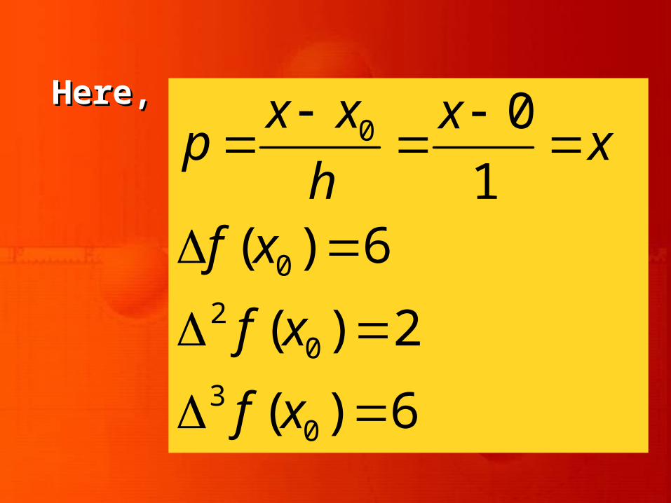
0

0

20

30

0

1( ) 6

( ) 2

( ) 6

x x xp x

hf x

f x

f x

Here,Here,

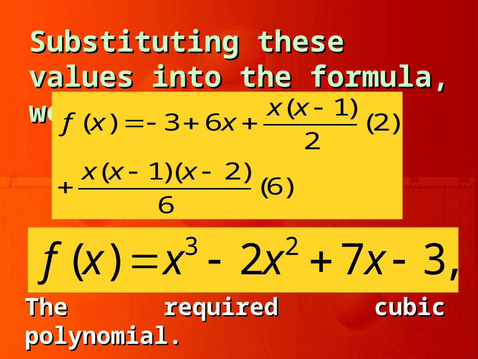
Substituting these values into Substituting these values into the formula, we havethe formula, we have

( 1)( ) 3 6 (2)

2( 1)( 2)

(6)6

x xf x x

x x x

The required cubic polynomial. The required cubic polynomial.

3 2( ) 2 7 3,f x x x x

NEWTON’S NEWTON’S BACKWARD BACKWARD DIFFERENCE DIFFERENCE

INTERPOLATION INTERPOLATION FORMULAFORMULA

For interpolating the value of For interpolating the value of the function the function yy = = ff ( (xx) near the ) near the end of table of values, and to end of table of values, and to extrapolate value of the extrapolate value of the function a short distance function a short distance forward from forward from yynn, Newton’s , Newton’s

backward interpolation backward interpolation formula is usedformula is used

DerivationDerivation

Let Let yy = = f f ((xx) be a function ) be a function which takes on values which takes on values f f ((xxnn), ), f f ((xxnn-h), -h), f f ((xxnn-2h), …, -2h), …, f f (x(x00)) corresponding to equispaced corresponding to equispaced values values xxnn, , xxnn--hh, , xxnn-2-2hh, …, , …, xx00. .

Suppose, we wish to evaluate Suppose, we wish to evaluate the function the function ff ( (xx) at () at (xxnn + + phph), ),

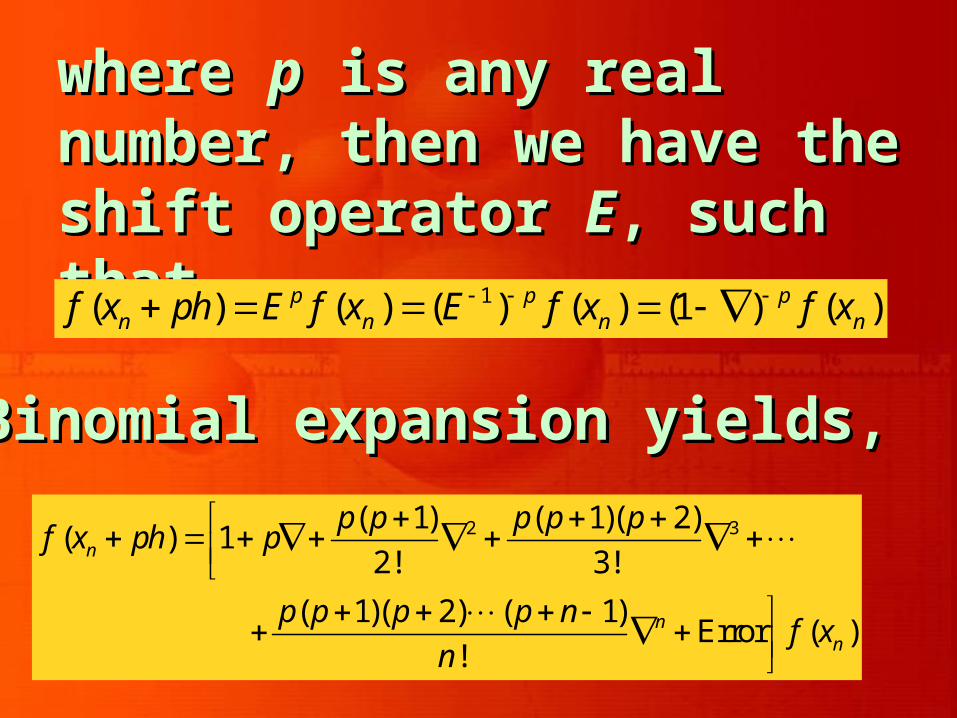
where where pp is any real number, is any real number, then we have the shift then we have the shift operator operator EE, such that , such that

1( ) ( ) ( ) ( ) (1 ) ( )p p pn n n nf x ph E f x E f x f x

Binomial expansion yields,Binomial expansion yields,

2 3( 1) ( 1)( 2)( ) 1

2! 3!

( 1)( 2) ( 1)Error ( )

!

n

nn

p p p p pf x ph p

p p p p nf x

n

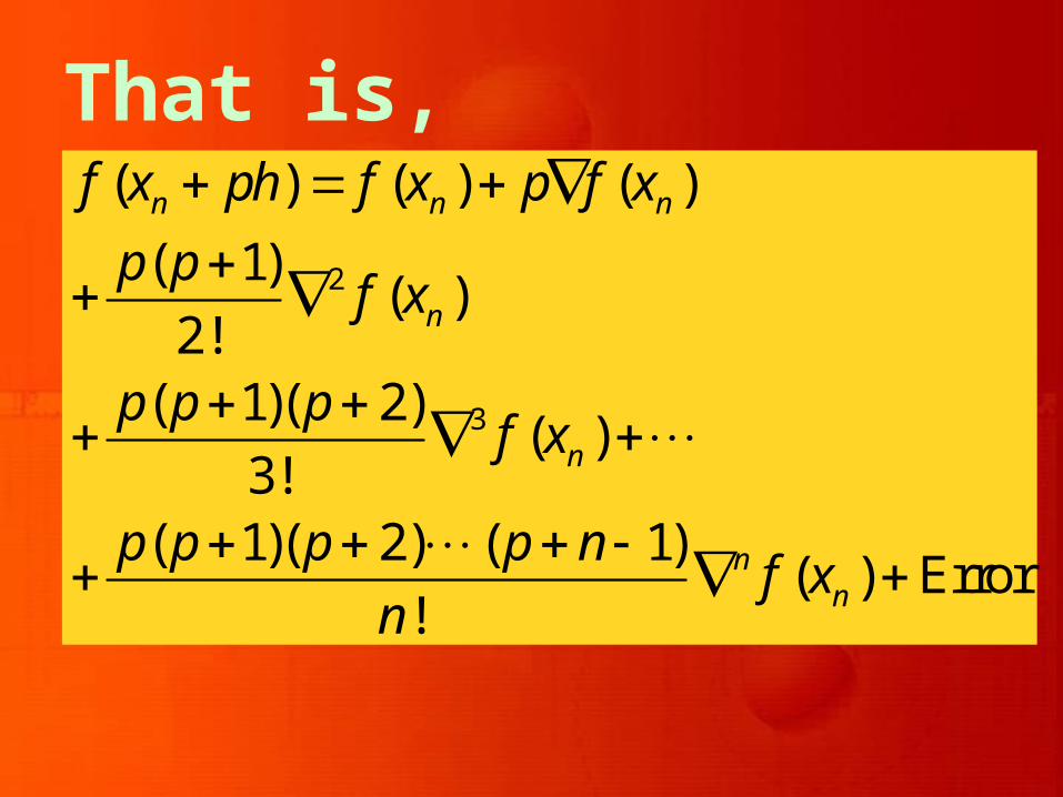
That is,

2

3

( ) ( ) ( )

( 1)( )

2!( 1)( 2)

( )3!

( 1)( 2) ( 1)( ) Error

!

n n n

n

n

nn

f x ph f x p f x

p pf x

p p pf x

p p p p nf x

n

This formula is known as This formula is known as Newton’s backward Newton’s backward interpolation formula. This interpolation formula. This formula is also known as formula is also known as Newton’s-Gregory backward Newton’s-Gregory backward difference interpolation difference interpolation formula. formula.

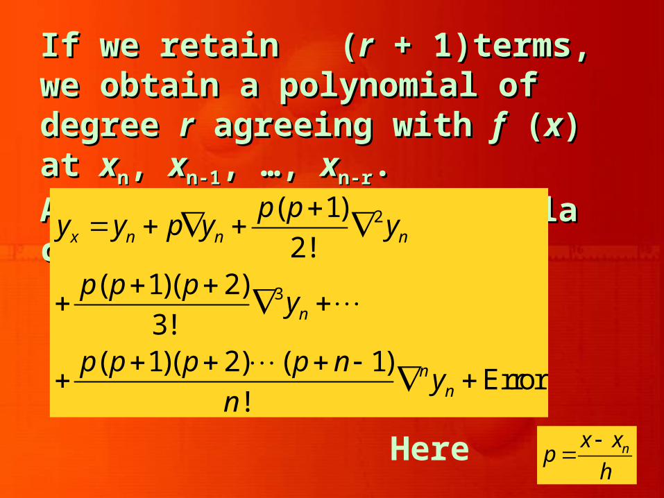
If we retain (If we retain (rr + 1)terms, we obtain a + 1)terms, we obtain a polynomial of degree polynomial of degree rr agreeing with agreeing with ff ( (xx) at ) at xxnn, , xxn-1n-1, …, , …, xxn-rn-r. Alternatively, . Alternatively,

this formula can also be written asthis formula can also be written as2

3

( 1)

2!( 1)( 2)

3!( 1)( 2) ( 1)

Error!

x n n n

n

nn

p py y p y y

p p py

p p p p ny

n

nx xp

h

Here

ExampleExample

For the following table of For the following table of values, estimate values, estimate ff (7.5). (7.5).

SolutionSolutionThe value to be interpolated is The value to be interpolated is at the end of the table. Hence, it at the end of the table. Hence, it is appropriate to use Newton’s is appropriate to use Newton’s backward interpolation formula. backward interpolation formula. Let us first construct the Let us first construct the backward difference table for backward difference table for the given datathe given data

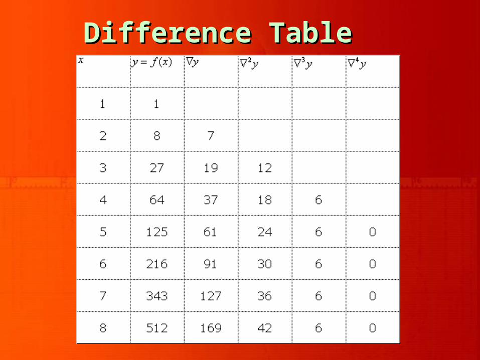
Difference TableDifference Table

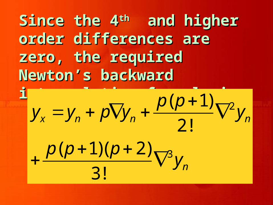
Since the 4Since the 4thth and higher order and higher order differences are zero, the required differences are zero, the required Newton’s backward interpolation Newton’s backward interpolation formula isformula is

2

3

( 1)

2!( 1)( 2)

3!

x n n n

n

p py y p y y

p p py

7.5 8.00.5

1nx x

ph

In this problem,In this problem,

2 3169, 42, 6n n ny y y

7.5

( 0.5)(0.5)512 ( 0.5)(169) (42)

2( 0.5)(0.5)(1.5)

(6)6

512 84.5 5.25 0.375

421.875

y

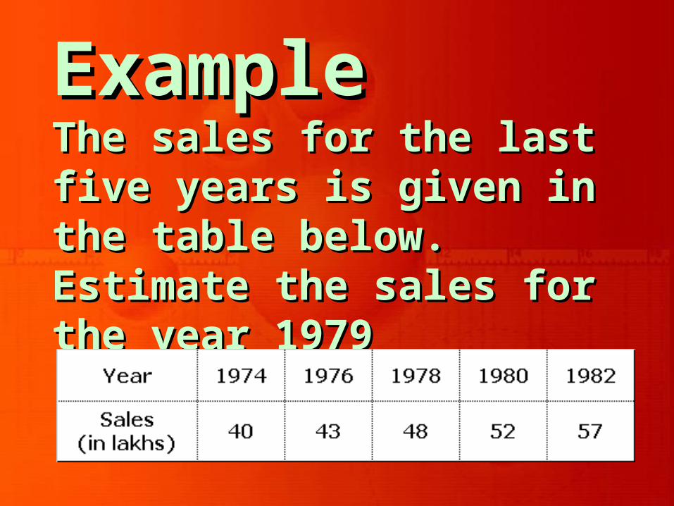
ExampleExampleThe sales for the last five The sales for the last five years is given in the table years is given in the table below. Estimate the sales for below. Estimate the sales for the year 1979the year 1979

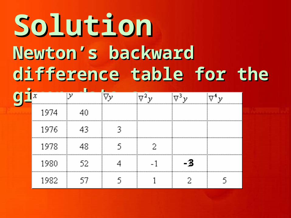
SolutionSolutionNewton’s backward difference Newton’s backward difference table for the given data astable for the given data as

-3

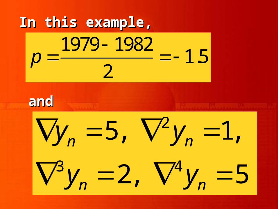
In this example,In this example,

1979 19821.5

2p

2

3 4

5, 1,

2, 5

n n

n n

y y

y y

andand

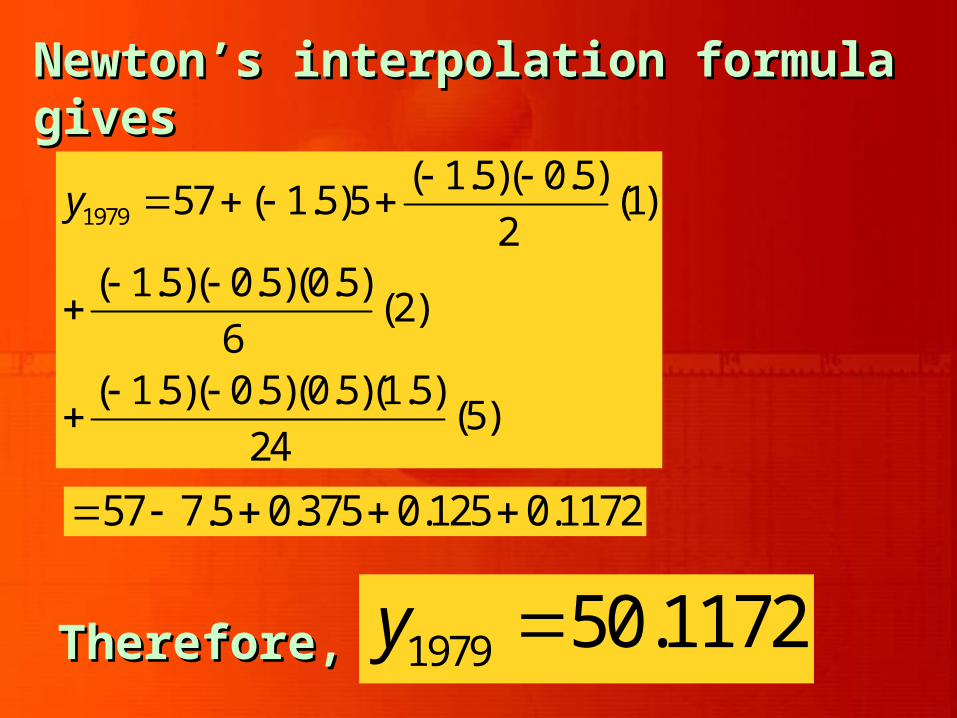
Newton’s interpolation formula givesNewton’s interpolation formula gives

1979

( 1.5)( 0.5)57 ( 1.5)5 (1)

2( 1.5)( 0.5)(0.5)

(2)6

( 1.5)( 0.5)(0.5)(1.5)(5)

24

y

57 7.5 0.375 0.125 0.1172

Therefore,Therefore, 1979 50.1172y

LAGRANGE’S LAGRANGE’S INTERPOLATION INTERPOLATION

FORMULAFORMULA

Newton’s interpolation Newton’s interpolation formulae developed earlier formulae developed earlier can be used only when the can be used only when the values of the independent values of the independent variable variable xx are equally are equally spaced. Also the spaced. Also the differences of differences of yy must must ultimately become small. ultimately become small.

If the values of the If the values of the independent variable are independent variable are not given at equidistant not given at equidistant intervals, then we have the intervals, then we have the basic formula associated basic formula associated with the name of Lagrange with the name of Lagrange which will be derived now.which will be derived now.

Lecture 22Lecture 22

NumericalAnalysis

NumericalAnalysis

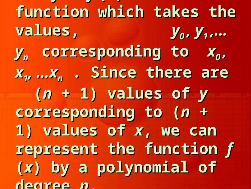
Let Let yy = = f f ((xx) be a function ) be a function which takes the values, which takes the values, yy0 0 , y, y1 1 ,…y,…ynn corresponding to corresponding to xx0 0

, x, x11, …x, …xnn . Since there are ( . Since there are (nn + +

1) values of 1) values of yy corresponding corresponding to (to (nn + 1) values of + 1) values of xx, we can , we can represent the function represent the function ff ( (xx) by ) by a polynomial of degree a polynomial of degree nn..

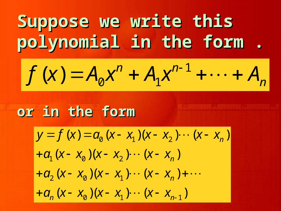
Suppose we write this Suppose we write this polynomial in the form .polynomial in the form .

10 1( ) n n

nf x A x A x A

or in the formor in the form

0 1 2

1 0 2

2 0 1

0 1 1

( ) ( )( ) ( )

( )( ) ( )

( )( ) ( )

( )( ) ( )

n

n

n

n n

y f x a x x x x x x

a x x x x x x

a x x x x x x

a x x x x x x

Here, the coefficients Here, the coefficients aakk are so are so

chosen as to satisfy this chosen as to satisfy this equation by the (equation by the (nn + 1) pairs + 1) pairs ((xxii, , yyii). Thus we get). Thus we get

0 0 0 0 1 0 1 0 2 0( ) ( )( )( ) ( )ny f x a x x x x x x x x

00

0 1 0 2 0( )( ) ( )n

ya

x x x x x x

Therefore,Therefore,

Similarly, we obtainSimilarly, we obtain

11

1 0 1 2 1( )( ) ( )n

ya

x x x x x x

0 1 1 1( )( ) ( )( ) ( )i

ii i i i i i i n

ya

x x x x x x x x x x

0 1 1( )( ) ( )n

nn n n n

ya

x x x x x x

andand

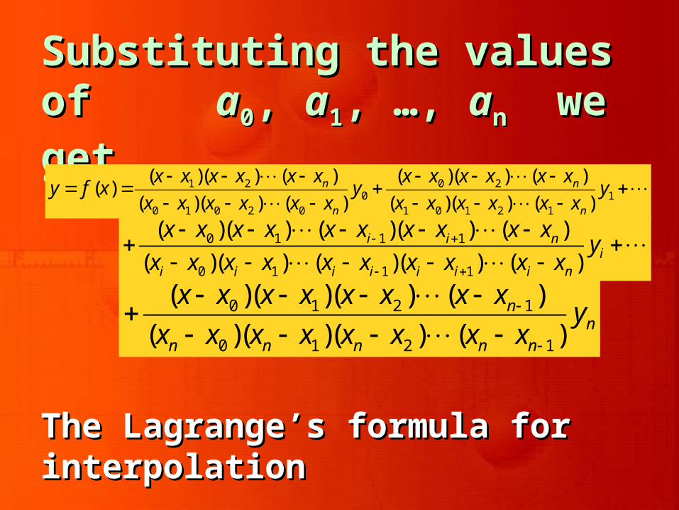
Substituting the values of Substituting the values of aa00, , aa11, …, , …, aann we get we get

1 2 0 20 1

0 1 0 2 0 1 0 1 2 1

( )( ) ( ) ( )( ) ( )( )

( )( ) ( ) ( )( ) ( )n n

n n

x x x x x x x x x x x xy f x y y

x x x x x x x x x x x x

0 1 1 1

0 1 1 1

( )( ) ( )( ) ( )

( )( ) ( )( ) ( )i i n

ii i i i i i i n

x x x x x x x x x xy

x x x x x x x x x x

0 1 2 1

0 1 2 1

( )( )( ) ( )

( )( )( ) ( )n

nn n n n n

x x x x x x x xy

x x x x x x x x

The Lagrange’s formula for The Lagrange’s formula for interpolationinterpolation

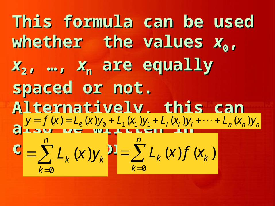
This formula can be used This formula can be used whetherwhether the values the values xx00, , xx22, …, , …, xxnn

are equally spaced or not. are equally spaced or not. Alternatively, this can also be Alternatively, this can also be written in compact form aswritten in compact form as

0 0 1 1 1( ) ( ) ( ) ( ) ( )i i i n n ny f x L x y L x y L x y L x y

0

( )n

k kk

L x y

0

( ) ( )n

k kk

L x f x

Where,Where,

0 1 1 1

0 1 1 1

( )( ) ( )( ) ( )( )

( )( ) ( )( ) ( )i i n

ii i i i i i i n

x x x x x x x x x xL x

x x x x x x x x x x

We can easily observe that, We can easily observe that, ( ) 1i iL x andand ( ) 0, .i jL x i j

Thus introducing Thus introducing KroneckerKronecker delta notationdelta notation

1, if( )

0, ifi j ij

i jL x

i j

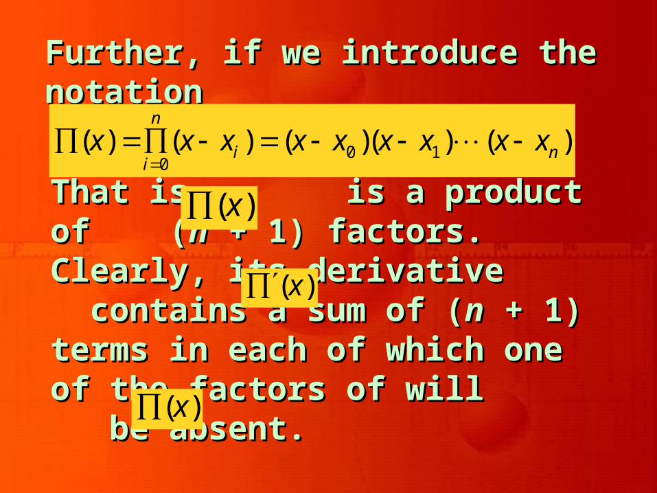
Further, if we introduce the Further, if we introduce the notationnotation

0 10

( ) ( ) ( )( ) ( )n

i ni

x x x x x x x x x

That is is a product of That is is a product of ((nn + 1) factors. Clearly, its + 1) factors. Clearly, its derivative contains a sum derivative contains a sum of (of (nn + 1) terms in each of + 1) terms in each of which one of the factors of which one of the factors of will be absent. will be absent.

( )x

( )x

( )x

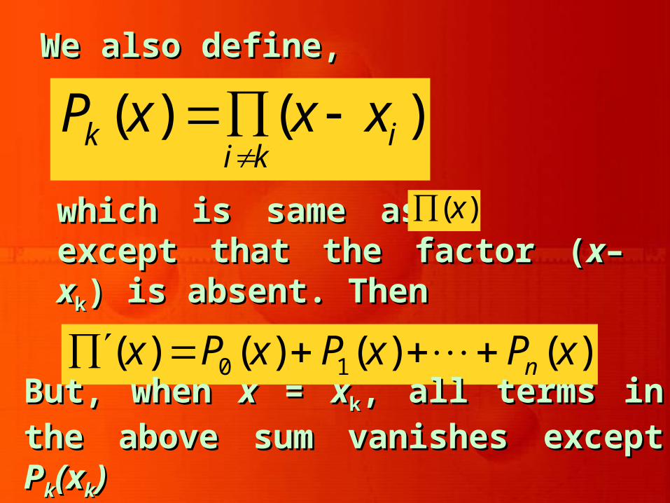
We also define,We also define,

( ) ( )k ii k

P x x x

which is same as except which is same as except that the factor (that the factor (xx––xxkk) is ) is absent. Thenabsent. Then

( )x

0 1( ) ( ) ( ) ( )nx P x P x P x But, when But, when xx = = xxkk, all terms in the , all terms in the above sum vanishes except above sum vanishes except PPkk(x(xkk))

Hence,Hence,

0 1 1( ) ( ) ( ) ( )( ) ( )k k k k k k xk k k nx P x x x x x x x x

( ) ( )( )

( ) ( )

( )

( ) ( )

k kk

k k k

k k

P x P xL x

P x x

x

x x x

Finally, the Lagrange’s Finally, the Lagrange’s interpolation polynomial of interpolation polynomial of degree n can be written asdegree n can be written as

0

0 0

( )( ) ( ) ( )

( ) ( )

( ) ( ) ( )

n

kk k k

n n

k k k kk k

xy x f x f x

x x x

L x f x L x y

ExampleExampleFind Lagrange’s Find Lagrange’s interpolation polynomial interpolation polynomial fitting the points fitting the points yy(1) = -3, (1) = -3, yy(3) = 0, (3) = 0, yy(4) = 30, (4) = 30, yy(6) = 132. (6) = 132. Hence find Hence find yy(5).(5).

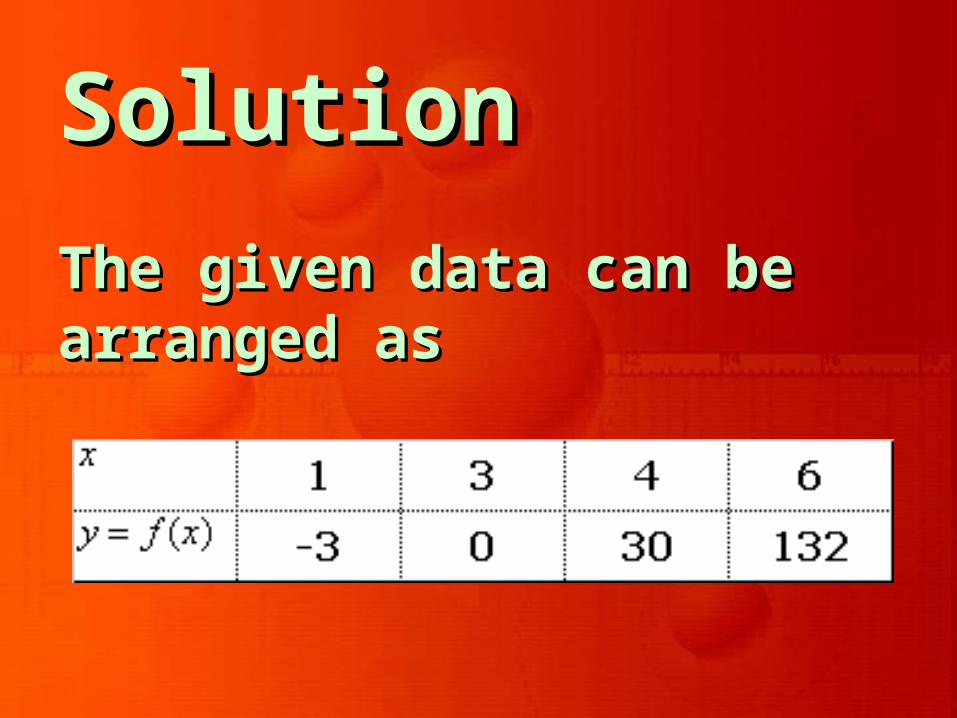
SolutionSolution

The given data can be The given data can be arranged asarranged as

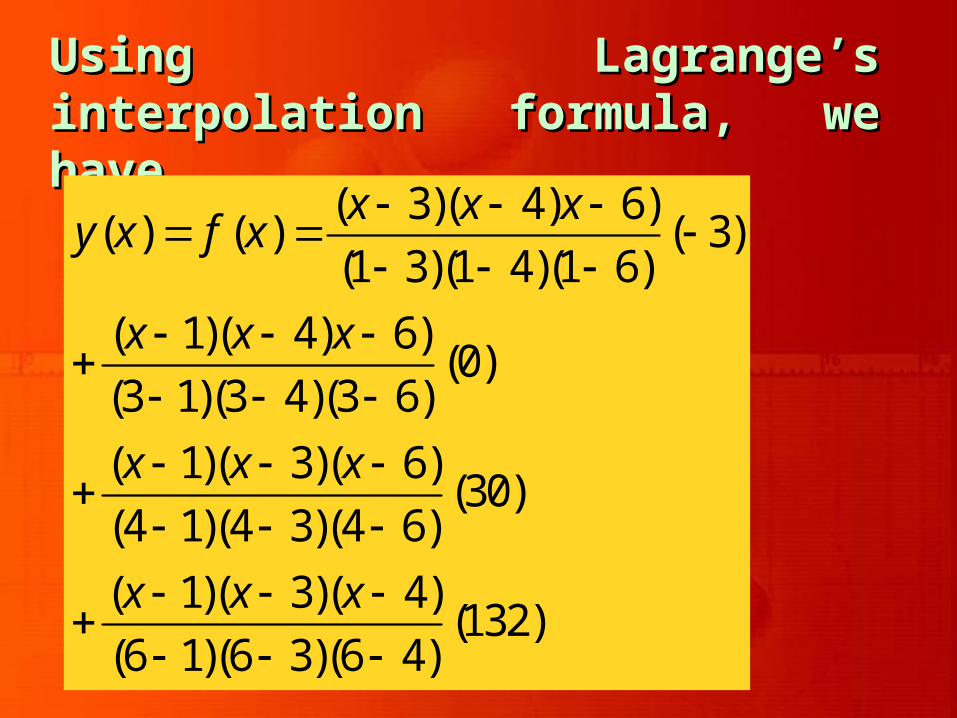
Using Lagrange’s Using Lagrange’s interpolation formula, we interpolation formula, we havehave

( 3)( 4) 6)( ) ( ) ( 3)

(1 3)(1 4)(1 6)

( 1)( 4) 6)(0)

(3 1)(3 4)(3 6)

( 1)( 3)( 6)(30)

(4 1)(4 3)(4 6)

( 1)( 3)( 4)(132)

(6 1)(6 3)(6 4)

x x xy x f x

x x x

x x x

x x x

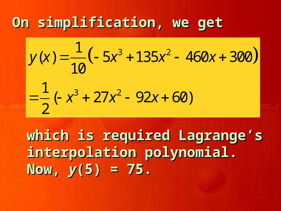
On simplification, we getOn simplification, we get

3 2

3 2

1( ) 5 135 460 300

101

( 27 92 60)2

y x x x x

x x x

which is required Lagrange’s which is required Lagrange’s interpolation polynomial. interpolation polynomial. Now, Now, yy(5) = 75.(5) = 75.

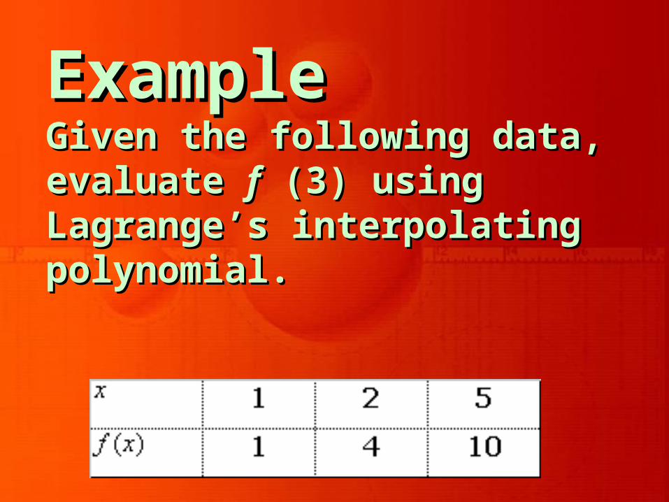
ExampleExampleGiven the following data, Given the following data, evaluate evaluate ff (3) using (3) using Lagrange’s interpolating Lagrange’s interpolating polynomial.polynomial.

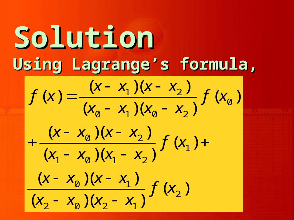
1 20

0 1 0 2

0 21

1 0 1 2

0 12

2 0 2 1

( )( )( ) ( )

( )( )

( )( )( )

( )( )

( )( )( )

( )( )

x x x xf x f x

x x x x

x x x xf x

x x x x

x x x xf x

x x x x

SolutionSolutionUsing Lagrange’s formula,Using Lagrange’s formula,

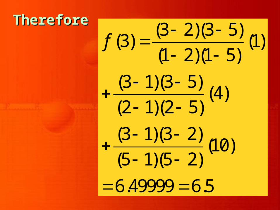
(3 2)(3 5)(3) (1)

(1 2)(1 5)

(3 1)(3 5)(4)

(2 1)(2 5)

(3 1)(3 2)(10)

(5 1)(5 2)

6.49999 6.5

f

ThereforeTherefore