lecture # 12: illumination, imaging, and particle image...

Copyright © by Dr. Hui Hu @ Iowa State University. All Rights Reserved!

Dr. Hui Hu

Department of Aerospace Engineering

Iowa State University

Ames, Iowa 50011, U.S.A

Lecture # 12: Illumination, imaging, and particle image

velocimetry

AerE 344 Lecture Notes

Sources/ Further reading: Hecht, “Optics” 4th ed.

Raffel, Willert, Wereley, Kompenhans, “Particle image velocimetry: A practical guide” 2nd ed.


The nature of light – as photons

Photon scattering:

• one finds experimentally that the frequency of the scattered wave is changed,

which does not come out of a wave picture of light. However, when the light is

viewed as a photon with energy proportional to the associated light wave,

excellent agreement with experiment is found.

The photoelectric effect:

• When light shines on a metal plate, electrons are ejected. These electrons are

accelerated to a nearby plate by an external potential difference, and a

photoelectric current is established, as below

• The photons hit an electron in the metal, giving up energy. If photon energy is

sufficient to free the electron, it is accelerated towards the other side; hence, a

flow of charges (current).

• The photoelectric current depends critically on the frequency of the light. This

is a feature of the energy that the electrons gain when struck by the light.

– in the wave description, the energy of the light depends on the

amplitude, and not on the frequency.

– however, in the photon description of light, the energy of the photon is

proportional to the frequency of the associated wave, which provides a

natural explanation of the frequency dependence of the photoelectric

current.

• The explanation was first given by Einstein and won him the Nobel Prize. JsconstPlanck

h3410624.6


Light Scattering

• Scattering

– Scattering is a general physical process whereby

some forms of radiation, such as light, are forced

to deviate from a straight trajectory by one or

more localized non-uniformities in the medium

through which it passes.

• Elastic Scattering

– Excited electron or atoms emits a photo have

exact the same frequency as the incident one.

• Inelastic scattering

– Excited electron or atoms emits a photo have a

frequency different from the incident one.


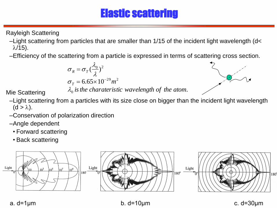
Elastic scattering

Rayleigh Scattering

–Light scattering from particles that are smaller than 1/15 of the incident light wavelength (d< /15).

–Efficiency of the scattering from a particle is expressed in terms of scattering cross section.

Mie Scattering

–Light scattering from a particles with its size close on bigger than the incident light wavelength (d > ).

–Conservation of polarization direction

–Angle dependent

• Forward scattering

• Back scattering

.

1065.6

)(

0

229

20

atomtheofwavelengthticcharateristheis

mT

TR

a. d=1μm b. d=10μm c. d=30μm


Inelastic Scattering

Raman Scattering

– Inelastic scattering from molecules.

– Chance to occur is about 10-5 ~ 10-2 of times lower than the Rayleigh scattering

– Scattering cross section is several orders smaller than the Rayleigh scattering

– Stoke transition : the energy of the emitted photon is higher than the absorbed photo.

– Anti-stoke transition: the energy of the emitted photon is lower than the absorbed photo.

– Time between the absorption and emission: 10-14 s.

– Anti-stokes line will be stronger when the temperature is low.


Fluorescence and phosphorescence

– Rayleigh and Raman scattering occurs essentially instantaneously. Not allowing other energy conversion phenomena to occur.


– Photoluminescence with time delay

Fluorescence

– Emission when the excited from singlet state to ground,

– lifetime is about 10-10 ~ 10-5 s.

Rhodamine B



Phosphorescence

– Emission when the excited atom or molecule

from triplet state to ground,

– lifetime is about 10-4 ~ 10-5 s.

0

1000

2000

3000

4000

5000

200 300 400 500 600 700 800

T = 32.0oC

T= 25.4 o

CT= 19.7

oC

T= 14.5oC

T = 10.2oC

T= 3.40 oC

Wavelength (nm)

Rel

ativ

e in

tens

ity

Spectraphotometer Output vs Wavelength

fluorescence

Phosphorescence

MTV chemical: 1-BrNp•M-CD•ROH complex


Absorption

Light is transmitted through a material, it will be

absorbed by the molecules of the material

Beer’s law:

• is the absorption or attenuation coefficient

•Lc=1/ is called penetration depth.

•When L=Lc, I/I0=1/e=37%, i.e., 63% energy was

absorbed

•Metals have very small Lc=1/.

– Copper, Lc=0.6nm for 100 nm UV light

– Copper, Lc=6.0nm for 1000 nm infrared light.

– 2nm copper plate as a low pass filter.

)exp(0 LII

L

I0


Illumination

Light sources:

• Thermal source:

– Lamps: Continuous wave (CW)

– Flash lamps (Pulsed)

– Arc lamps

• Laser sources

– Continuous wave (CW)

– Pulsed laser

– Singe wavelength

• Point source:

• Plane source:


Light source

• Thermal light source:

–Emit electromagnetic radiation as a result of being heated to

high-temperature

–Line sources:

–Continuum sources:

• Incandescent lamps: heated tungsten filament in a evacuated

glass container.

• Electric discharge lamps: fluorescent lamps. Filled with

mercury vapor at low pressure and utilize an electric discharge

through it to produce light in ultraviolet (UV) range. Through

fluorescent, it is convert to visible light.

• Flash lamps: tubes containing a noble gas such xenon,

krypton or argon. For their operation, high voltage stored in a

capacitor is discharged through the gas, producing a highly

luminous corona discharge. Light pulse is about 1s to1 ms.

• Sparks: produced by the electric breakdown of a gas (helium,

neo, argon or air) during an electric discharge between

electrodes. The choice of different electrodes produces sparks

of different shapes.

http://images.google.com/imgres?imgurl=http://www.me-dtc.com/images/heavy_duty_incandescent.jpg&imgrefurl=http://www.me-dtc.com/product_line/incandescent_page_mouseover.htm&h=432&w=261&sz=28&hl=en&start=7&tbnid=sza1b1qs5VS6oM:&tbnh=126&tbnw=76&prev=/images%3Fq%3DIncandescent%2Blamps%26svnum%3D10%26hl%3Den%26rls%3DGGLJ,GGLJ:2006-12,GGLJ:en%26sa%3DN


Laser

• Laser: Light Amplification by Stimulated Emission of Radiation

(LASER)

• Advantages of laser light over thermal light source:

–Coherent light (with all light wave front in phase)

–Collimated and concentrated (parallel light with small cross

area)

–Monochromic (energy concentrated in a very narrow

wavelength band)

• How a laser works:

–Radiation energy is produced by an activated medium( can

be gas, crystal or semiconductor or liquid solution).

–The medium consists of particles (atom, ions or molecules).

–When a photo, having energy hv, approaching the particles,

the photo may be absorbed cause an electron or atoms to

be raised temporarily to high-energy level.

–When the excited electron or molecule to return ground

level, spontaneous emission or stimulated emission would

take place.


Laser

–Spontaneous emission: emit a photo with the same

energy as that absorbed one, but in random direction.

–Stimulated emission: An electron or atom is already at a

higher energy level could become excited by an incident

photo, without absorb the photo, it will emission another

photo with identical energy (frequency), phase, and

direction as the incident photon.

–External power source is required to maintain the

population of the atoms in higher energy level in order to

make to stimulated emission taking place continuously.

–Optical cavity.

–Q-switch


Commonly used Lasers

–Helium-neon (He-Ne) laser

• Active medium is helium neon atoms

• Continuous wave laser

• Power 0.3 ~15 mW

• =633nm (red)

–Argon-ion (Ar-ion) laser

• Active medium is argon atoms maintained at the ion

state.

• Continuous wave laser

• Power level: 100 mW ~10 W

• Have seven wavelengths

• =488n (blue)

• =514.5nm (green)

• LDV application

• LIF in liquid flows



–Nd-YAG laser

• Solid-state laser

• Active medium: neodymium (Nd+3) as active medium

incorporated as an impurity into a crystal of Yattium-

Aluminium-Garnet (YAG) as a host

• Flash lamp is used as external source

• pulsed laser: 10 -400mJ/pulse or more

• Pulse duration: 100ps ~ 10ns

• Wavelenght of tube =1064nm (infrared)

• SHG: =532nm (green), THG: =355nm (UV), FHG:

=266nm (deepUV)

• PIV, MTV, PLIF

• Repetition rate can be as high as 30 Hz.



–Copper Vapor laser

• Active medium: copper vapor

• Pulsed laser: 10mJ/pulse or more

• Pulse duration: 15 ~ 60ns

• =510.6nm (green), =578.2nm (yellow)

• Repetition rate can be as high as f=5,000~15,000 Hz.

• High-speed PIV, LIF and others

–Dye laser

• Active medium: complex multi-atomic organic molecules

• =200nm ~ 1500nm

–Excimer laser

• Gas laser KrF and Xecl

• High-energy

• UV wavelength

• Pulsed laser

• high repetition frequency


Light sensing and recording


Lenses

• Focal length: f

• f/# , “F-number”: defined as the

ratio of focal distance of the lens

and its clear aperture diameter.

• Depth of focus H = 2 ∙f/# ∙ c ∙ Z/f


Photodetector

• Photo detector is a device to convert light to an electric

current through photo electric effect.

• Quantum efficiency:

• Noise:

– Shot noise: due to random fluctuation of the rate of

photon collection and back ground illumination

– Thermal noise: caused by amplification of current

inside the photo detector and by external amplifier.

• Dark current: the current produced by the photo detector

even in the absence of a desirable light source.

• Two kinds of photo detectors:

– Photomultiplier tubes (PMT)

– photodiodes (PD) or photo electric cells

electrons emitted ofNumber :

photons absorbed ofNumber :

p

e

p

eq

N

N

N

N


Photodetector

• photodiodes (PD) or photo electric cells

– P-n junctions of semiconductors,

commonly silicon-silicon type.

– High quantum efficiency

– But not internal amplification

http://ccd.mii.cz/image?id=559


Interlaced Cameras

The fastest response time of human being for images is about ~ 15Hz

Video format:

• PAL (Phase Alternating Line ) format with frame rate of f=25Hz (sometimes in 50Hz). Used by U.K., Germany, Spain, Portugal, Italy, China, India, most of Africa, and the Middle East

• NTSC format: established by National Television Standards Committee (NTSC) with frame rate of f=30Hz. Used by U.S., Canada, Mexico, some parts of Central and South America, Japan, Taiwan, and Korea.

Even field

(2,4,6…640)

Old field

(1,3,5…639)

Even field

Odd field

16.6ms 16.6ms

1 frame

F=30Hz

480 pixels by 640 pixels

Interlaced camera

time


Progressive scan camera

• All image systems produce a clear

image of the background

• Jagged edges from motion with

interlaced scan

• Motion blur caused by the lack of

resolution in the 2CIF sample

• Only progressive scan makes it

possible to identify the driver


Mystery of flying rods


Electronic shutter modes

• Rolling shutter: The sensor is exposed line by line. Each of the pixels integrate light for the

specified exposure time; however, not all pixels are exposing at the same time. The start time

for each pixel’s exposure is a function of sensor position. This mode is typical of large formate

sensors, such as digital SLR cameras.

• Global shutter: Each pixel integrates light for the specified exposure time simultaneously. This

method is preferred for capturing highly dynamic events. This mode is typical of high-speed

CMOS cameras which can operate at frame rates beyond 1 million frames per second.

Rolling shutter Gobal shutter

Point Grey Cameras Point Grey Cameras


Particle-based Flow Diagnostic Techniques

• Seeded the flow with small particles (~ µm in size)

• Assumption: the particle tracers move with the same velocity as local flow

velocity!

Flow velocity

Vf

Particle velocity

Vp =

Measurement of

particle velocity


Particle-based techniques: Particle Image Velocimetry (PIV)

• To seed fluid flows with small tracer particles (~µm), and assume the tracer particles

moving with the same velocity as the low fluid flows.

• To measure the displacements (L) of the tracer particles between known time

interval (t). The local velocity of fluid flow is calculated by U= L/t .

A. t=t0 B. t=t0+10 s C. Derived Velocity field

X (mm)

Y(m

m)

-50 0 50 100 150

-60

-40

-20

0

20

40

60

80

100

-0.9 -0.7 -0.5 -0.3 -0.1 0.1 0.3 0.5 0.7 0.9

5.0 m/sspanwisevorticity (1/s)

shadow region

GA(W)-1 airfoil

t=t0 t

LU

t= t0+t L


PIV System Setup

Illumination system

(Laser and optics)

camera

Synchronizer

seed flow with

tracer particles

Host computer

Particle tracers: track the fluid movement.

Illumination system: illuminate the flow field in the interest region.

Camera: capture the images of the particle tracers.

Synchronizer: control the timing of the laser illumination and camera acquisition.

Host computer: to store the particle images and conduct image processing.


Tracer Particles for PIV

• Tracer particles should be neutrally buoyant and small enough to follow the flow perfectly.

• Tracer particles should be big enough to scatter the illumination lights efficiently .

• The scattering efficiency of trace particles also strongly depends on the ratio of the

refractive index of the particles to that of the fluid.

For example: the refractive index of water is considerably larger than that of air.

The scattering of particles in air is at least one order of magnitude more

efficient than particles of the same size in water.

h

Incident light Scattering light

a. d=1μm b. d=10μm c. d=30μm



18

);exp(1()(

18

)(

2

2

p

ps

s

p

p

pPs

d

tUtU

gdUUU

U

gdUp

pg

18

)(2

PU


• Tracers for PIV measurements in liquids (water):

• Polymer particles (d=10~100 m, density = 1.03 ~ 1.05 kg/cm3)

• Silver-covered hollow glass beams (d =1 ~10 m, density = 1.03 ~ 1.05 kg/cm3)

• Fluorescent particle for micro flow (d=200~1000 nm, density = 1.03 ~ 1.05 kg/cm3).

•Quantum dots (d= 2 ~ 10 nm)

• Tracers for PIV measurements in gaseous flows:

• Smoke …

• Droplets, mist, vapor…

• Condensations ….

• Hollow silica particles (0.5 ~ 2 μm in diameter and 0.2 g/cm3 in density for PIV

measurements in combustion applications.

•Nanoparticles of combustion products



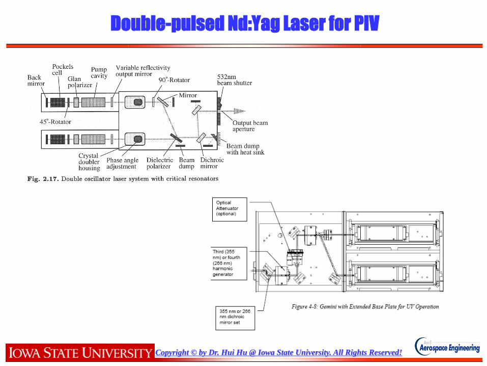
Illumination system

• The illumination system of PIV is always composed of light source and optics.

• Lasers: such as Argon-ion laser and Nd:YAG Laser, are widely used as light

source in PIV systems due to their ability to emit monochromatic light with high

energy density which can easily be bundled into thin light sheet for illuminating

and recording the tracer particles without chromatic aberrations.

• Optics: always consist of a set of cylindrical lenses and mirrors to shape the

light source into a planar sheet to illuminate the flow field.

laser optics

Laser beam

Laser sheet


Double-pulsed Nd:Yag Laser for PIV


Optics for PIV


Cameras

• Types of cameras for PIV:

• Photographic film-based cameras (old)

•Charged-coupled device (CCD) cameras

•High speed Complementary metal-oxide semiconductor (CMOS) cameras

•Advantages of digital cameras:

• It is fully digitized

• Various digital techniques can be implemented for PIV image processing.

• Conventional auto- or cross- correlation techniques combined with special

framing techniques can be used to measure higher velocities.

• Disadvantages of digital cameras:

• Low temporal resolution (defined by the video framing rate):

• Low spatial resolution:


Synchronizer

• Function of Synchronizer:

• To control the timing of the laser illumination and camera acquisition

• “Frame straddling” strategy for two-frame single exposure recordings

1st

pulsed

2nd

pulsed

Timing of

pulsed laser

Timing of

CCD camera

time

1st frame exposure

2nd frame exposure

t

33.33ms

(30Hz)

To laser To camera

From computer

Synchronizer


Host computer

• To send timing control parameter to synchronizer.

• To store the particle images and conduct image processing.

Host computer

To synchronizer

Image data from camera


Single-frame technique

particle

Streak line

V L=V*t

single-pulse Multiple-pulse

Particle streak velocimetry

http://www.pbase.com/andrej_z/weekly_assignment


Multi-frame technique

a. T=t0

b. T=t1

c. T=t2

a. T=t3

t=t0

t

LU

t= t0+t

L


Example PIV raw data

In-plane

U

Δζ, Δz

Image: A B


U

h

Through-plane In-plane Trefftz

plane

Example PIV raw data


Image Processing for PIV

• To extract velocity information from particle images.

t=t0 t=t0+4ms

A typical PIV raw image pair

Y/D

X/D

-2 -1 0 1 2 31

1.5

2

2.5

3

3.5

4

4.5

5

1.1001.0501.0000.9500.9000.8500.8000.7500.7000.6500.6000.5500.5000.4500.4000.3500.3000.2500.2000.1500.100

Velocity U/Uin

Image processing


Particle Tracking Velocimetry (PTV)

t=t0 t=t0+t

Low particle-image

density case

1. Find position of the particles at each

images

2. Find corresponding particle image pair

in the different image frame

3. Find the displacements between the

particle pairs.

4. Velocity of particle equates the

displacement divided by the time

interval between the frames.


Particle Tracking Velocimetry (PTV)-2

Particle position of time step t=t1

Search region for

time step t=t4

Search region for time step t=t3

Search region for time step t=t2

Four-frame-particle

tracking algorithm

1. Find position of the particles at each

images

2. Find corresponding particle image pair

in the different image frame

3. Find the displacements between the

particle pairs.

4. Velocity of particle equates the

displacement divided by the time

interval between the frames.

PTV results


Correlation-based PIV methods

high particle-image density

t=t0 t=t0+t

Corresponding flow

velocity field


Correlation-based PIV methods

t=t0 t=t0+t

dvgyxgdvfyxf

dvgyxgfyxfqpR

22

)),(()),((

)),(()),((,

Correlation coefficient function:


Cross Correlation Operation

Signal A:

Signal B:

dxuxgdxxf

dxuxgxfuR

])([*])([

)](*)([

22


1 4 7 10 13 16 19 22 25 28 31S1

S10

S19

S280.7

0.75

0.8

0.85

0.9

0.95

1

Correlation coefficient distribution

dvgyxgdvfyxf

dvgyxgfyxfqpR

22

)),(()),((

)),(()),((,

R(p,q)

Peak location


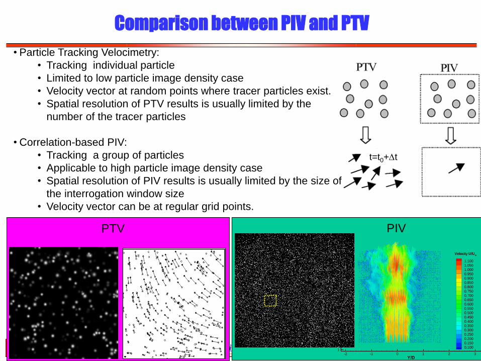
Comparison between PIV and PTV

• Particle Tracking Velocimetry:

• Tracking individual particle

• Limited to low particle image density case

• Velocity vector at random points where tracer particles exist.

• Spatial resolution of PTV results is usually limited by the

number of the tracer particles

• Correlation-based PIV:

• Tracking a group of particles

• Applicable to high particle image density case

• Spatial resolution of PIV results is usually limited by the size of

the interrogation window size

• Velocity vector can be at regular grid points.

PTV

t=t0+t

PIV

Y/D

X/D

-2 -1 0 1 2 31

1.5

2

2.5

3

3.5

4

4.5

5

1.1001.0501.0000.9500.9000.8500.8000.7500.7000.6500.6000.5500.5000.4500.4000.3500.3000.2500.2000.1500.100

Velocity U/Uin


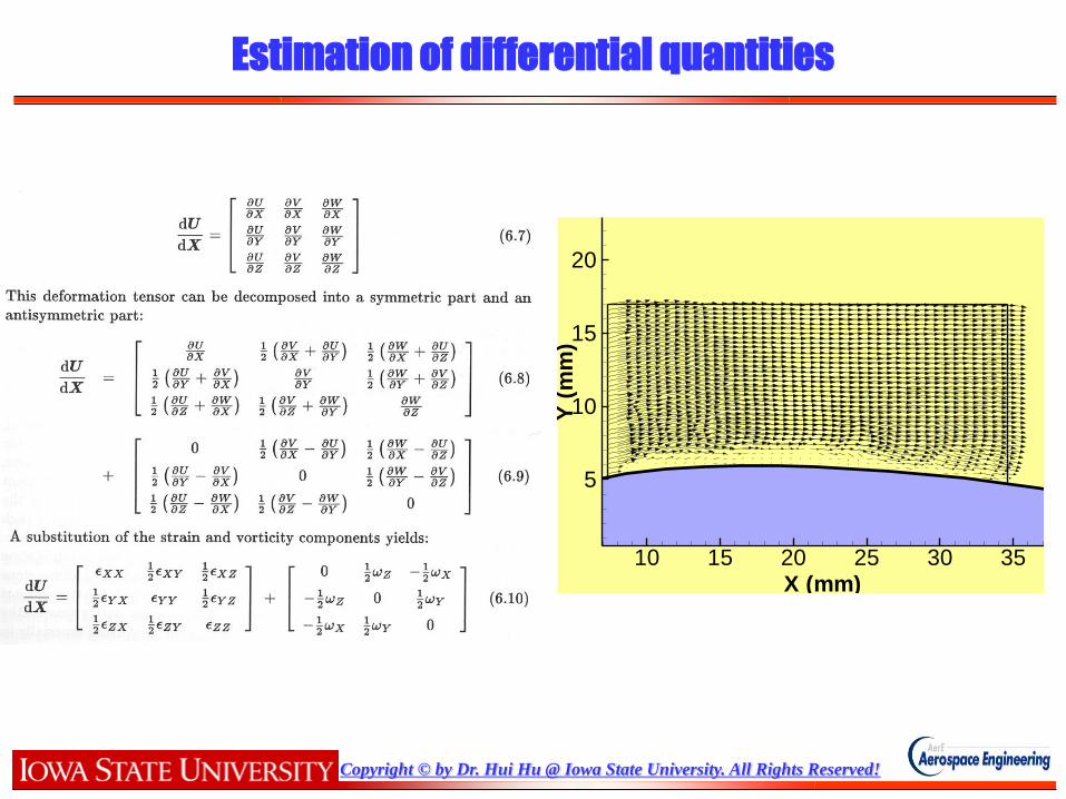
Estimation of differential quantities

X (mm)Y

(mm

)10 15 20 25 30 35

5

10

15

20


Estimation of differential quantities


Estimation of Vorticity distribution

y

U

x

Vz


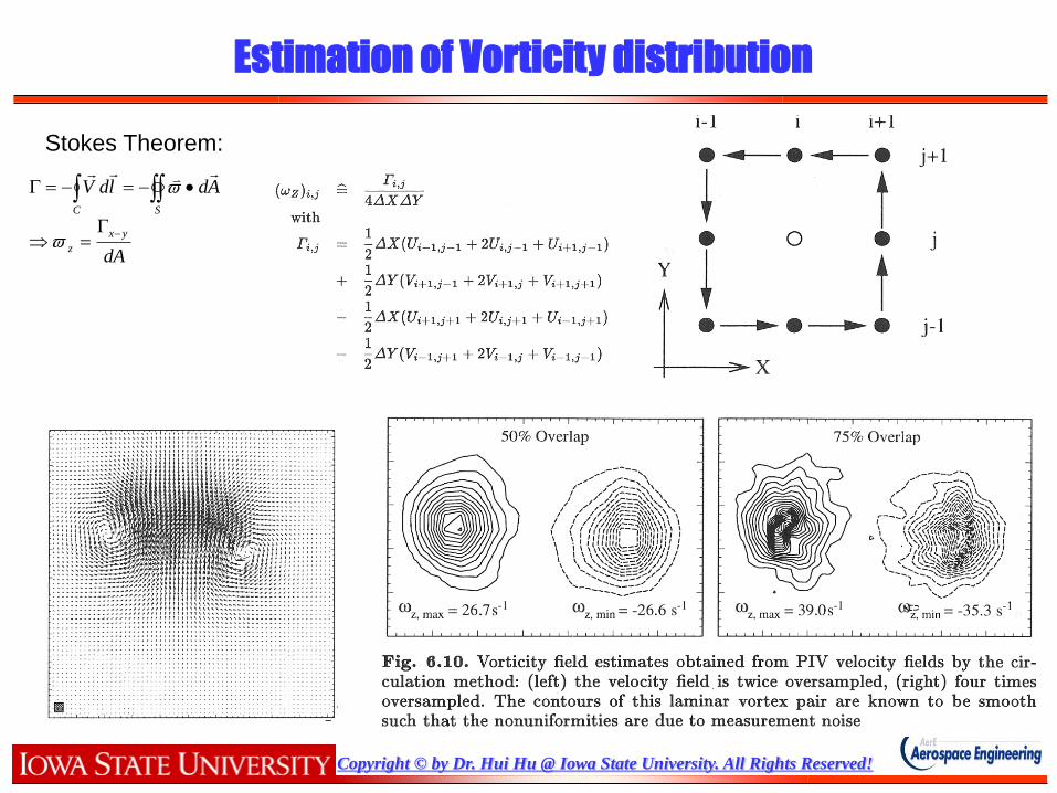
Estimation of Vorticity distribution

Stokes Theorem:

dA

AdldV

yx

z

C S


Vorticity distribution Examples

-50 0 50 100 150 200 250 300-50

0

50

100

150

200

250

-25.00 -20.00 -15.00 -10.00 -5.00 0.00 5.00 10.00 15.00 20.00 25.00

Spanwise Vorticity ( Z-direction )

Re =6,700

Uin = 0.33 m/s

X mm

Ym

m

Uo

ut

water free surface

X (mm)

Y(m

m)

-20 0 20 40 60 80 100 120 140

-60

-40

-20

0

20

40

60 -3.2 -2.7 -2.2 -1.7 -1.2 -0.7 -0.2 0.3 0.8 1.3 1.8

10 m/sspanwisevorticity (1/s)

shadow region

GA(W)-1 airfoil


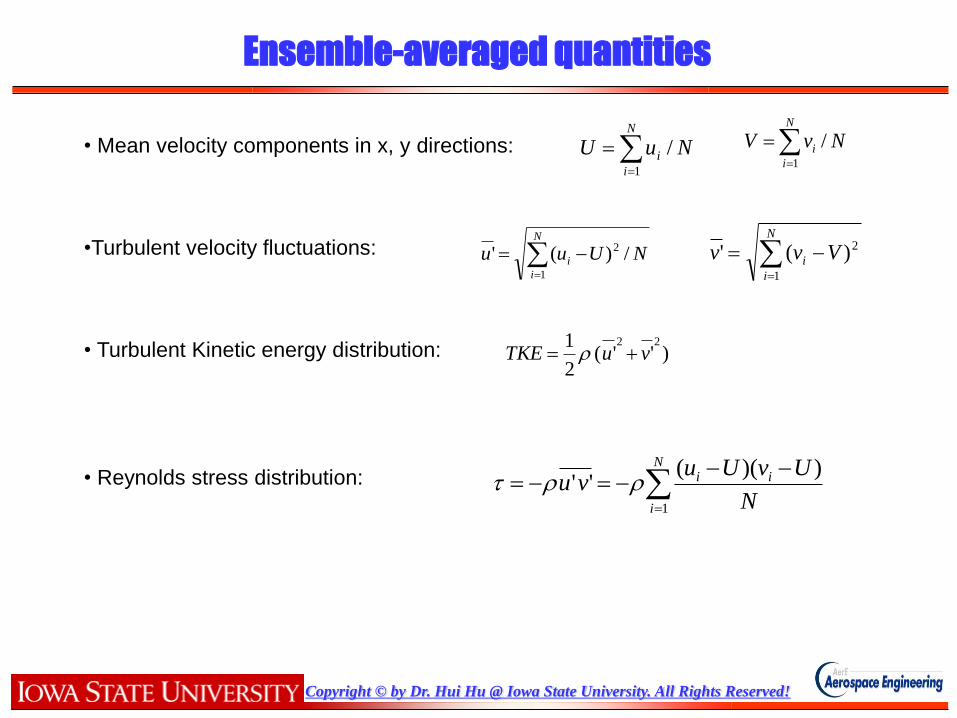
Ensemble-averaged quantities

• Mean velocity components in x, y directions:

•Turbulent velocity fluctuations:

• Turbulent Kinetic energy distribution:

• Reynolds stress distribution:

NUuuN

i

i /)('1

2

N

i

i Vvv1

2)('

N

i

i NuU1

/

N

i

i NvV1

/

)''(2

1 22

vuTKE

N

i

ii

N

UvUuvu

1

))((''


Ensemble-averaged quantities

X (mm)

Y(m

m)

-20 0 20 40 60 80 100 120 140

-60

-40

-20

0

20

40

60 U m/s: -1.0 1.0 3.0 5.0 7.0 9.0 11.0 13.0 15.0

10 m/s

shadow region

GA(W)-1 airfoil

X (mm)

Y(m

m)

-20 0 20 40 60 80 100 120 140

-60

-40

-20

0

20

40

60 vort: -3.0 -2.0 -1.0 0.0 1.0 2.0 3.0

10 m/s

shadow region

GA(W)-1 airfoil

X (mm)

Y(m

m)

-20 0 20 40 60 80 100 120 140

-60

-40

-20

0

20

40

60 -0.035 -0.025 -0.015 -0.005 0.005 0.015 0.025 0.035

shadow region

GA(W)-1 airfoil

NormalizedReynolds Stress

X (mm)

Y(m

m)

-20 0 20 40 60 80 100 120 140

-60

-40

-20

0

20

40

60 0.010 0.020 0.030 0.040 0.050 0.060 0.070 0.080 0.090 0.100

shadow region

GA(W)-1 airfoil

T.K.E


Pressure field estimation

)(1

)(1

2

2

2

2

2

2

2

2

y

v

x

v

y

p

y

vv

x

vu

y

u

x

u

x

p

y

uv

x

uu


Integral Force estimation

FVdfAdPAdVVVdVt

VCSCSCVC

........

~)(

X (mm)

Y(m

m)

-20 0 20 40 60 80 100 120 140

-60

-40

-20

0

20

40

60 U m/s: -1.0 1.0 3.0 5.0 7.0 9.0 11.0 13.0 15.0

10 m/s

shadow region

GA(W)-1 airfoil


Tank with compressed air Test section

AerE344 Lab: Pressure Measurements in a de Laval Nozzle

Tap No. Distance downstream of throat (inches) Area (Sq. inches)

1 -4.00 0.8002 -1.50 0.5293 -0.30 0.4804 -0.18 0.4785 0.00 0.4766 0.15 0.4977 0.30 0.5188 0.45 0.5399 0.60 0.56010 0.75 0.58111 0.90 0.59912 1.05 0.61613 1.20 0.62714 1.35 0.63215 1.45 0.634


1st, 2nd, and 3rd critical conditions

Under-

expanded

flow

Flow close to

3rd critical

Over-

expanded

flow

2nd critical – shock

is at nozzle exit

Over-expanded flow

with shock between

nozzle exit and

throat

1st critical – shock

is almost at the

nozzle throat.

lecture # 12: illumination, imaging, and particle image...

Documents