lecture 15: flood mitigation and forecast modelinglecture 15: flood mitigation and forecast...
TRANSCRIPT

Lecture 15: Flood Mitigation and Forecast ModelingKey Questions1. What is a 100-year flood inundation map?
2. What is a levee and a setback levee?
3. How are land acquisition, insurance, emergency response used to mitigate a flood
4. How is streamflow forecasting used to mitigate a flood?
5. What is the difference between weather and climate?
6. What has caused the climate to change in the last 100 years?
7. How will future climate impact snow andstreamflow in the Nooksack basin?
Niigata Japan, 1964 liquefaction
Nooksack River

100-year Floodplain Map
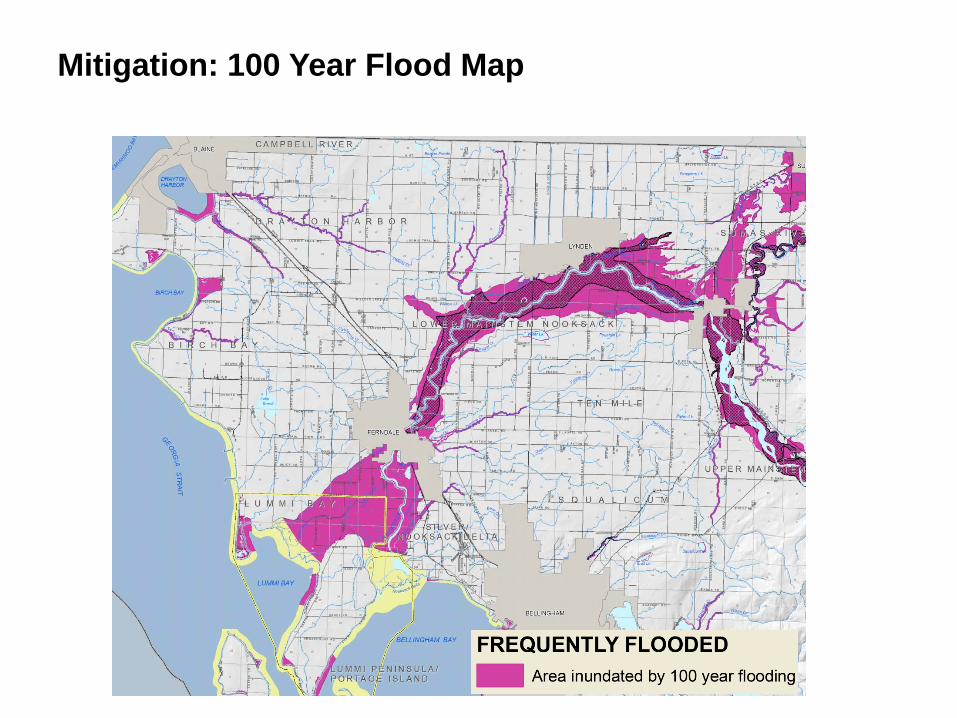
Mitigation: 100 Year Flood Map
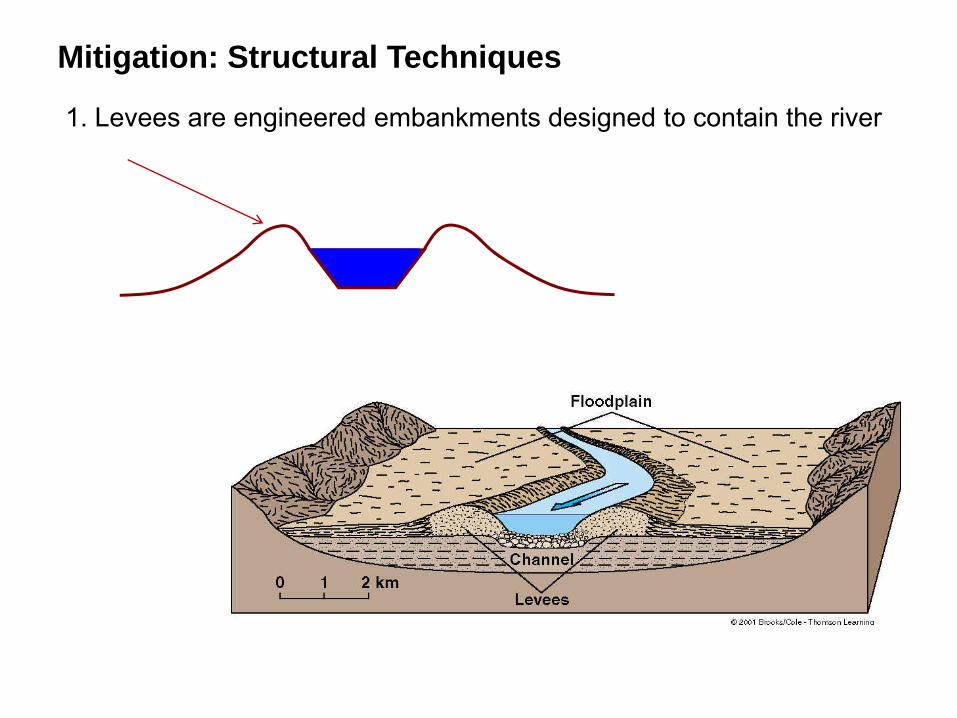
Mitigation: Structural Techniques
1. Levees are engineered embankments designed to contain the river

Mitigation: Structural Techniques
Levees are designed to contain floods along most of the lower Nooksack (floods that range from 5 to 100 year return periods)
levee
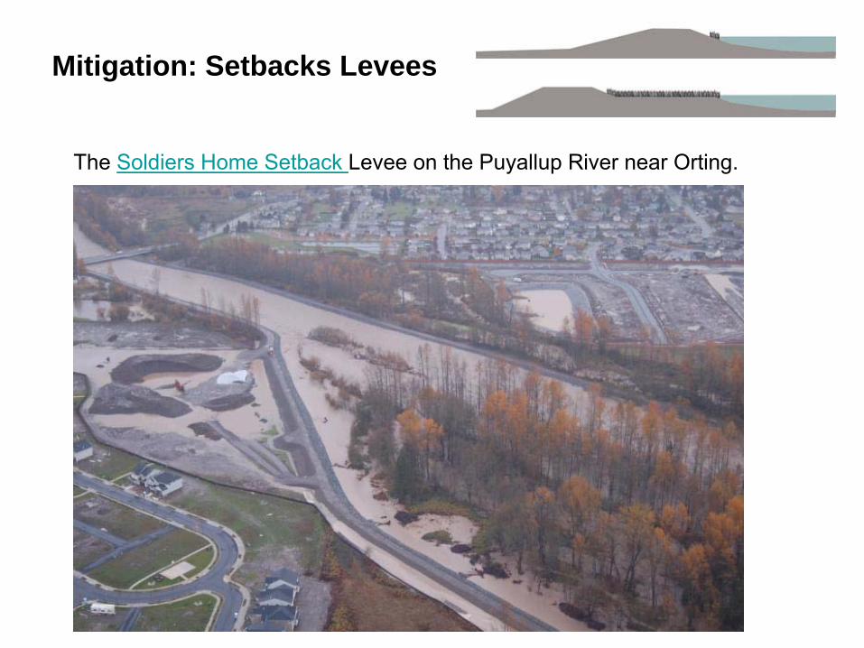
Mitigation: Setbacks Levees
The Soldiers Home Setback Levee on the Puyallup River near Orting.

Mitigation: Structural Techniques
2. Dams can store and slowly release water
storage capacity
monitored release
Δ
=

Mitigation: Land Acquisition


Mitigation: Forecast Modeling
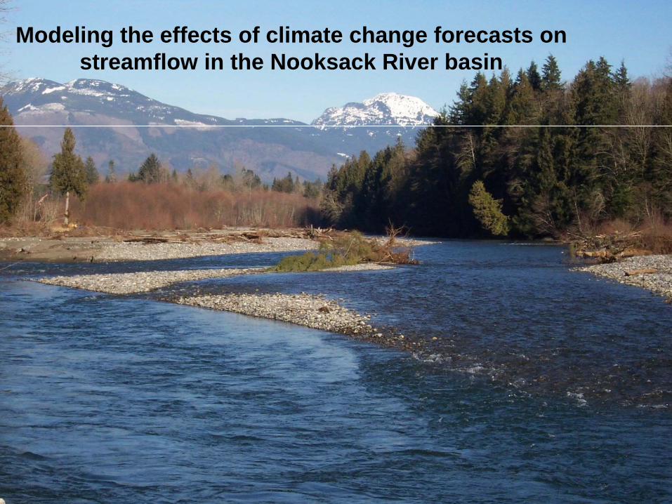
Modeling the effects of climate change forecasts on streamflow in the Nooksack River basin

Climate versus Weather
Weather: short-term, local variations in atmospheric conditions (one monthly average represents weather)
Average January temperatures at the Clearbrook weather station.

Climate versus Weather
Climate: long-term average weather conditions (30 years or longer)(collection of monthly values represents climate)
Average January temperatures at the Clearbrook weather station.
What does the trend line indicate?
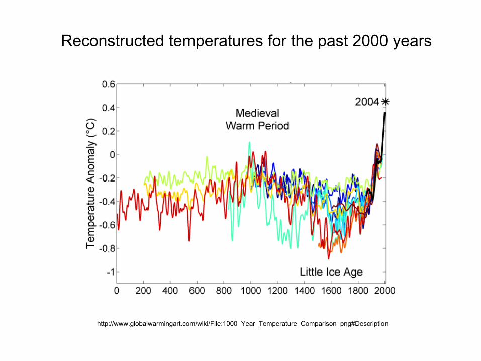
http://www.globalwarmingart.com/wiki/File:1000_Year_Temperature_Comparison_png#Description
Reconstructed temperatures for the past 2000 years

http://www.globalwarmingart.com/wiki/File:1000_Year_Temperature_Comparison_png#Description
Measured temperatures for the past 200 years

n = 3146
97% of active, publishing climatologists think human activities have changed the climate

Greenhouse Gases

Greenhouse Effect: CO2 and other greenhouse gases trap radiated heat from the Earth and increase the temperature
http://www.esrl.noaa.gov/gmd/outreach/carbon_toolkit/basics.html
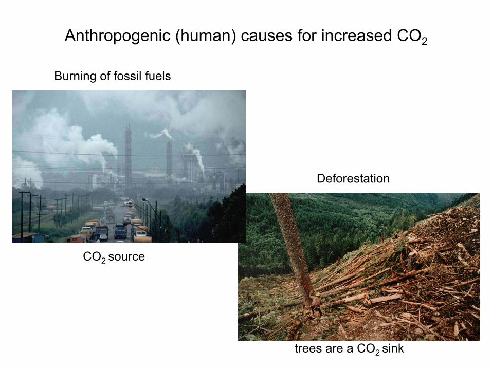
Anthropogenic (human) causes for increased CO2
Burning of fossil fuels
Deforestation
CO2 source
trees are a CO2 sink


South Cascade Glacier
1960
1928 2000
One of three benchmark Glaciers that have been established in a USGS glacier monitoring program

South Cascade Glacier
One of three benchmark Glaciers that have been established in a USGS glacier monitoring program

Mote et al. (2008)Averaged sea level at stable tide gauge sites

Futuristic CO2 Emission Scenarios

General Circulation Models (GCM)
Emission Scenarios
About 40 institutions world wide run GMCs

Modeled Temperature Predictions based on different CO2 emission scenarios

GCM: NASA’s GISS model

Modeling the effects of climate change forecasts on streamflow in the Nooksack River basin

Goal of ResearchTo predict impact of climate change on snowpack and streamflow in the Nooksack River basin
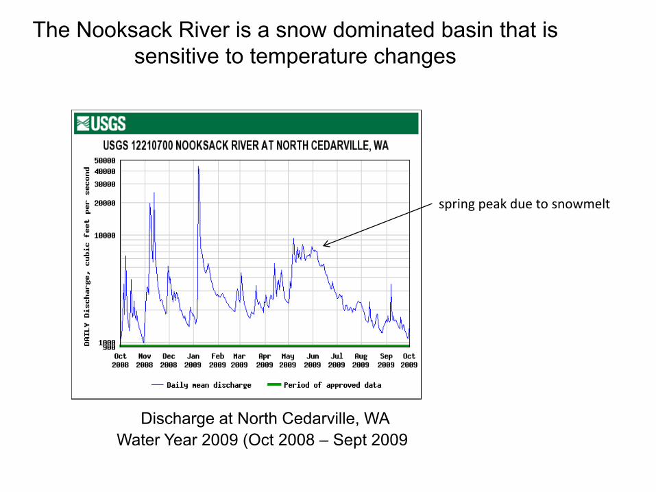
The Nooksack River is a snow dominated basin that is sensitive to temperature changes
Discharge at North Cedarville, WAWater Year 2009 (Oct 2008 – Sept 2009)
spring peak due to snowmelt

Time
Hydrograph
Time
Hydrograph
snow packno snowpack so rain falls on exposed bedrock and thin, wet soils and produces a high peak
more volume but less peaked
HydrographHydrograph
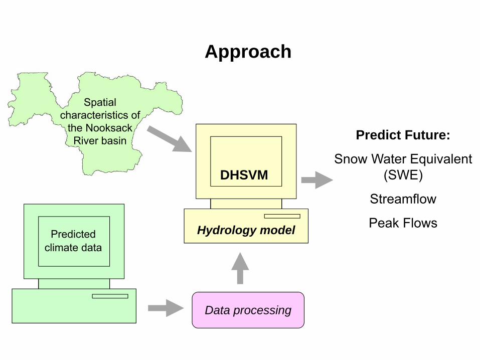
Approach
Predicted climate data
Predict Future:
Snow Water Equivalent (SWE)
Streamflow
Peak FlowsHydrology model
DHSVM
Spatial characteristics of
the Nooksack River basin
Data processing

Methods
1. Hydrologic Model Set-up, Calibration, & Validation
2. Downscaling & Validation of Climate Change Forecasts
3. Hydrologic Modeling

Methods: DHSVMDistributed Hydrology Soil Vegetation Model
DHSVM calculates a water and energy budget on each grid cell for each time step
inputs - outputs = change in storage

The DHSVM also predicts snow accumulation and melt

Methods: DHSVM
Spatial Input• DEM
• Watershed Boundary
• Stream Network
• Soil Thickness
• Soil Type
• Landcover

Methods: DHSVM
Meteorological Input• Temperature
• Precipitation
• Wind Speed
• Relative Humidity
• Shortwave Radiation
• Longwave Radiation
North Shore Weather Station, Lake Whatcom

DHSVM: Streamflow Calibration
Photo: USGS
Calibration – adjustment of model parameters to mimic an observed dataset
USGS Stream gauge at Cedarville

DHSVM: Calibration
Initial Simulation
After Calibration
010
000
3000
0
Nooksack River, WY 06-07
Date
Dai
ly M
ean
Stre
amflo
w (c
fs)
1Jan2006 2Jul2006 1Jan2007 2Jul2007
Cedarville - observedCedarville - simulated
010
000
3000
0
Nooksack River, WY 06-07
Date
Dai
ly M
ean
Stre
amflo
w (c
fs)
1Jan2006 2Jul2006 1Jan2007 2Jul2007
Cedarville - observedCedarville - simulated
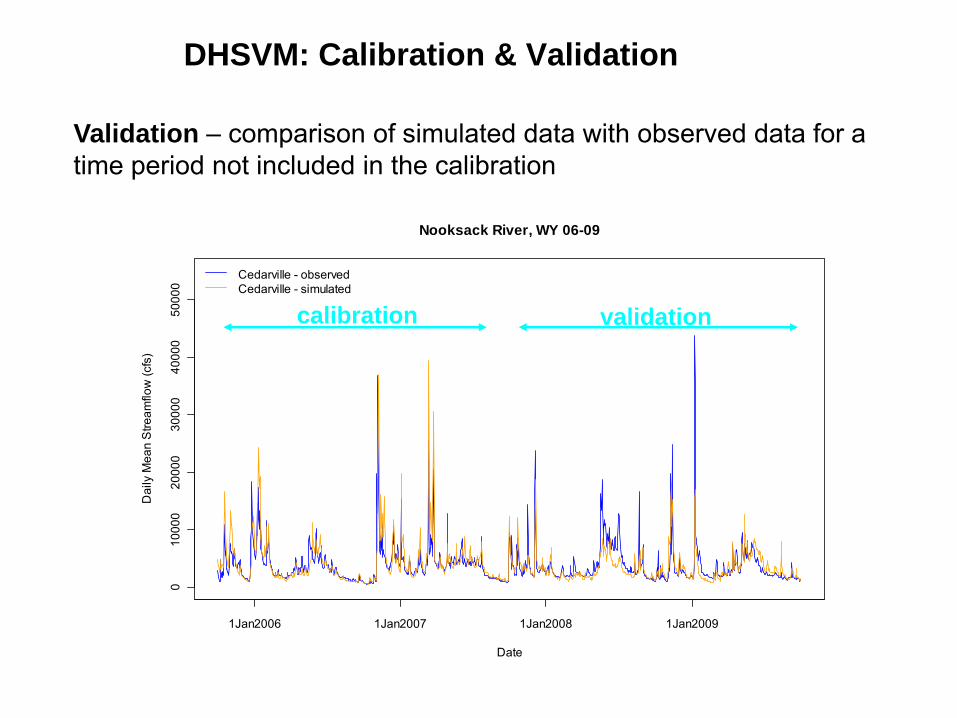
DHSVM: Calibration & Validation
Validation – comparison of simulated data with observed data for a time period not included in the calibration
010
000
2000
030
000
4000
050
000
Nooksack River, WY 06-09
Date
Dai
ly M
ean
Stre
amflo
w (c
fs)
1Jan2006 1Jan2007 1Jan2008 1Jan2009
Cedarville - observedCedarville - simulated
calibration validation

DHSVM: SWE Calibration
Photo: NRCS
Calibration – adjustment of model parameters to mimic an observed dataset
Snotel Stations

DHSVM: Calibration & Validation
01
23
4
Wells Creek Snotel (NF), WY 06-09
Date
Dai
ly M
ean
SW
E (m
)
1Jan2006 1Jan2007 1Jan2008 1Jan2009
observedsimulated
01
23
4
Middle Fork Snotel, WY 06-09
Date
Dai
ly M
ean
SW
E (m
)
1Jan2006 1Jan2007 1Jan2008 1Jan2009
observedsimulated

Methods
1. Hydrologic Model Set-up, Calibration, & Validation
2. Downscaling & Validation of Climate Change Forecasts
3. Hydrologic Modeling

IPCC 2001
Emissions Scenarios

Methods: Climate Change Forecasts
2040s Changes in Temperature and PrecipitationMote and others, 2005
Three General Circulation Models (GCMs) :
1. IPSL_CM4_A2Institut Pierre Simon Laplace (with A2)
2. Echam5_A2Max Planck Institute for Meteorology (with A2)
3. GISS_ER_B1Goddard Institute for Space Studies (with B1)

GCM scale of 100s km regional scale of 10s km local station
Methods: GCM Downscaling
CIG, 2010
Monthly time scale

Methods: GCM Downscaling
April Mean Temperature
Mean Temperature (C)
Freq
uenc
y
7 8 9 10 11 12
02
46
810
6 7 8 9 10 11 12
0.0
0.2
0.4
0.6
0.8
1.0
April eCDF
Mean Temperature (C)
Non
-Exc
eeda
nce
Pro
babi
lity
Abbotsford, 1950-1999
Empirical Cumulative Distribution Functions (eCDF)

Methods: GCM Downscaling
6 8 10 12 14
0.0
0.2
0.4
0.6
0.8
1.0
April eCDFs
Mean Temperature (C)
Non
-Exc
eeda
nce
Pro
babi
lity
Abbotsford, 1950-19992050s GISS Forecast, 2035-2065
Shift 50-year historical time series based on 31-year
forecast period
Result: 50-year forecast
6 8 10 12 14
0.0
0.2
0.4
0.6
0.8
1.0
April eCDFs
Mean Temperature (C)
Non
-Exc
eeda
nce
Pro
babi
lity
Abbotsford, 1950-1999GISS Forecast, 2035-2065Combined 2050s Forecast

Methods: GCM Downscaling
Each forecast is based on the Abbotsford time series
0 100 200 300 400 500 600
-10
010
2030
Monthly Mean Temperature, 1950-1999
Month
Tem
pera
ture
(C)
AbbotsfordGISS_B1 2050 Forecast

Methods: GCM Downscaling
Each forecast is based on the Abbotsford time series
0 100 200 300 400 500 600
-10
010
2030
Monthly Mean Temperature, 1950-1999
Month
Tem
pera
ture
(C)
AbbotsfordGISS_B1 2050 Forecast

Methods: Validation of Downscaling
1 2 3 4 5 6 7 8 9 10 11 12
-10
010
20
Monthly Mean Temperature, 1950-1999
Month
Tem
pera
ture
(C)
-10
010
20-1
00
1020
-10
010
20
AbbotsfordGISS_B1Echam_A2IPSL_A2
12
34
56
7
median
outlier
25th – 75th percentiles
minimum

Methods: Local Forecasts
1 2 3 4 5 6 7 8 9 10 11 12
-10
010
2030
Monthly Mean Temperature - 2050
Month
Tem
pera
ture
(C)
-10
010
2030
-10
010
2030
-10
010
2030
AbbotsfordGISS_B1ECHAM_A2IPSL_A2

Methods: Local Forecasts
1 2 3 4 5 6 7 8 9 10 11 12
010
020
030
040
050
060
0
Total Monthly Precipitation - 2050
Month
Pre
cipi
tatio
n (m
m)
010
020
030
040
050
060
00
100
200
300
400
500
600
010
020
030
040
050
060
0 AbbotsfordGISS_B1ECHAM_A2IPSL_A2

Methods: Processing of Forecasts
1. Apply monthly ΔT to daily Abbotsford data
2. Disaggregate daily data to a 3-hour time step
3. Derive other 3-hour meteorological input from temperature and precipitation
• Shortwave Radiation
• Longwave Radiation
• Windspeed
• Relative Humidity

Methods
1. Hydrologic Model Set-up, Calibration, & Validation
2. Downscaling & Validation of Climate Change Forecasts
3. Hydrologic Modeling

Approach
Predicted climate data
Predict Future:
Snow Water Equivalent (SWE)
Streamflow
Peak FlowsHydrology model
DHSVM
Spatial characteristics of
the Nooksack River basin
Data processing

Results: SWE
1 2 3 4 5 6 7 8 9 10 11 12
01
23
45
Monthly Mean SWE at MF Snotel - IPSL_A2
Month
SWE(
m)
1950-19992000202520502075
1 2 3 4 5 6 7 8 9 10 11 12
01
23
45
Monthly Mean SWE at MF Snotel - GISS_B1
Month
SWE(
m)
1950-19992000202520502075

Results: SWE
2 4 6 8 10 12
0.0
0.5
1.0
1.5
2.0
2.5
3.0
Monthly Mean SWE at MF Snotel - GISS_B1
Month
SWE
(m)
1950-19992000202520502075
2 4 6 8 10 12
0.0
0.5
1.0
1.5
2.0
2.5
3.0
Monthly Mean SWE at MF Snotel - IPSL_A2
Month
SWE
(m)
1950-19992000202520502075

Results: Streamflow
1 2 3 4 5 6 7 8 9 10 11 12
050
0010
000
1500
020
000
Monthly Median Streamflow - IPSL_A2
Month
Stre
amflo
w (c
fs)
1950-19992000202520502075
1 2 3 4 5 6 7 8 9 10 11 12
050
0010
000
1500
020
000
Monthly Median Streamflow - GISS_B1
Month
Stre
amflo
w (c
fs)
1950-19992000202520502075
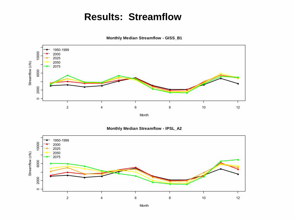
Results: Streamflow
2 4 6 8 10 12
020
0060
0010
000
Monthly Median Streamflow - IPSL_A2
Month
Stre
amflo
w (c
fs)
1950-19992000202520502075
2 4 6 8 10 12
020
0060
0010
000
Monthly Median Streamflow - GISS_B1
Month
Stre
amflo
w (c
fs)
1950-19992000202520502075

Results: Peak Flow Events
0e+0
04e
+04
8e+0
4
Annual Peak Flows (WY 1951-1999) - IPSL_A2
Stre
amflo
w (c
fs)
Ferndale-observedCedarville-simulated2000202520502075
0e+0
04e
+04
8e+0
4Annual Peak Flows (WY 1951-1999) - GISS_B1
Stre
amflo
w (c
fs)
Ferndale-observedCedarville-simulated2000202520502075

Results: Peak Flow Events
IPSL_A2 2000
Month
Freq
uenc
y
0 2 4 6 8 10
010
2030
40
IPSL_A2 2025
Month
Freq
uenc
y
0 2 4 6 8 10
010
2030
40
IPSL_A2 2050
Month
Freq
uenc
y
0 2 4 6 8 10
010
2030
40
IPSL_A2 2075
Month
Freq
uenc
y
0 2 4 6 8 10
010
2030
40
Simulated Peaks Above 30,000 cfs
Forecast Period
Freq
uenc
y
2000 2025 2050 2075
020
4060
8010
0
GISS_B1Echam_A2IPSL_A2

Temperature or Precipitation?
• Predicted increases in temperature and precipitation
• More agreement on temperature trends
• Previous regional studies indicate that temperature is the driving factor in changes to SWE(Hamlet et al., 2005, Mote et al., 2005, Mote et al., 2008)
1 2 3 4 5 6 7 8 9 10 11 12
-10
010
2030
Monthly Mean Temperature - 2075
Month
Tem
pera
ture
(C)
-10
010
2030
-10
010
2030
-10
010
2030
AbbotsfordGISS_B1ECHAM_A2IPSL_A2
1 2 3 4 5 6 7 8 9 10 11 12
010
020
030
040
050
060
0
Total Monthly Precipitation - 2075
Month
Pre
cipi
tatio
n (m
m)
010
020
030
040
050
060
00
100
200
300
400
500
600
010
020
030
040
050
060
0 AbbotsfordGISS_B1ECHAM_A2IPSL_A2
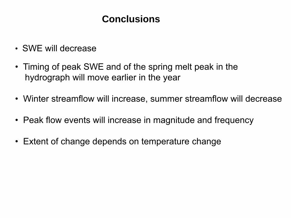
Conclusions
• SWE will decrease
• Timing of peak SWE and of the spring melt peak in the hydrograph will move earlier in the year
• Winter streamflow will increase, summer streamflow will decrease
• Peak flow events will increase in magnitude and frequency
• Extent of change depends on temperature change
Photo: John Scurlock
