lecture 16: geometric nonlinear control - umu.se...lecture 16: geometric nonlinear control •...
TRANSCRIPT
Lecture 16: Geometric Nonlinear Control
• Background and Useful Concepts
c©Anton Shiriaev. 5EL158: Lecture 16 – p. 1/21
Lecture 16: Geometric Nonlinear Control
• Background and Useful Concepts
• Feedback Linearization
c©Anton Shiriaev. 5EL158: Lecture 16 – p. 1/21
Lecture 16: Geometric Nonlinear Control
• Background and Useful Concepts
• Feedback Linearization
• Feedback Linearization for Single Link Flexible Joint
c©Anton Shiriaev. 5EL158: Lecture 16 – p. 1/21
A Smooth Manifold in Rn
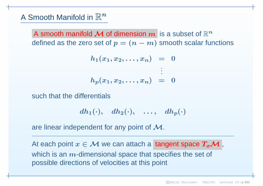
A smooth manifold M of dimension m is a subset of Rn
defined as the zero set of p = (n − m) smooth scalar functions
h1(x1, x2, . . . , xn) = 0...
hp(x1, x2, . . . , xn) = 0
such that the differentials
dh1(·), dh2(·), . . . , dhp(·)
are linear independent for any point of M.
c©Anton Shiriaev. 5EL158: Lecture 16 – p. 2/21
A Smooth Manifold in Rn
A smooth manifold M of dimension m is a subset of Rn
defined as the zero set of p = (n − m) smooth scalar functions
h1(x1, x2, . . . , xn) = 0...
hp(x1, x2, . . . , xn) = 0
such that the differentials
dh1(·), dh2(·), . . . , dhp(·)
are linear independent for any point of M.
At each point x ∈ M we can attach a tangent space TxM ,
which is an m-dimensional space that specifies the set ofpossible directions of velocities at this point
c©Anton Shiriaev. 5EL158: Lecture 16 – p. 2/21
Example
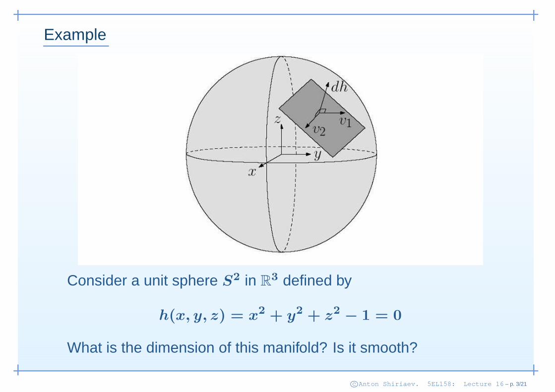
Consider a unit sphere S2 in R3 defined by
h(x, y, z) = x2 + y2 + z2 − 1 = 0
What is the dimension of this manifold? Is it smooth?
c©Anton Shiriaev. 5EL158: Lecture 16 – p. 3/21
Example
The differential dh(·) of the function
h(x, y, z) = x2 + y2 + z2 − 1 = 0
at the point (x0, y0, z0) ∈ S2 is the row vector
dh(x0, y0, z0) =[
∂∂x
h, ∂∂y
h, ∂∂z
h]∣∣∣x=x0, y=y0, z=z0
c©Anton Shiriaev. 5EL158: Lecture 16 – p. 3/21

Example
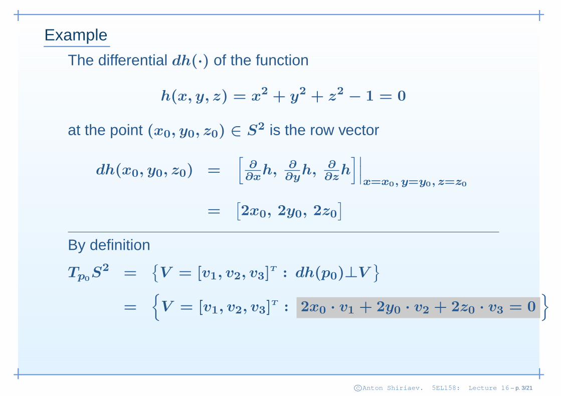
The differential dh(·) of the function
h(x, y, z) = x2 + y2 + z2 − 1 = 0
at the point (x0, y0, z0) ∈ S2 is the row vector
dh(x0, y0, z0) =[
∂∂x
h, ∂∂y
h, ∂∂z
h]∣∣∣x=x0, y=y0, z=z0
=[2x0, 2y0, 2z0
]
c©Anton Shiriaev. 5EL158: Lecture 16 – p. 3/21

Example
The differential dh(·) of the function
h(x, y, z) = x2 + y2 + z2 − 1 = 0
at the point (x0, y0, z0) ∈ S2 is the row vector
dh(x0, y0, z0) =[
∂∂x
h, ∂∂y
h, ∂∂z
h]∣∣∣x=x0, y=y0, z=z0
=[2x0, 2y0, 2z0
]
How to compute a tangent space Tp0S2 to the sphere S2
at the point p0 = (x0, y0, z0) ∈ S2?
c©Anton Shiriaev. 5EL158: Lecture 16 – p. 3/21
Example
The differential dh(·) of the function
h(x, y, z) = x2 + y2 + z2 − 1 = 0
at the point (x0, y0, z0) ∈ S2 is the row vector
dh(x0, y0, z0) =[
∂∂x
h, ∂∂y
h, ∂∂z
h]∣∣∣x=x0, y=y0, z=z0
=[2x0, 2y0, 2z0
]
By definition
Tp0S2 =
V = [v1, v2, v3]
T : dh(p0)⊥V
=
V = [v1, v2, v3]T : 2x0 · v1 + 2y0 · v2 + 2z0 · v3 = 0
c©Anton Shiriaev. 5EL158: Lecture 16 – p. 3/21
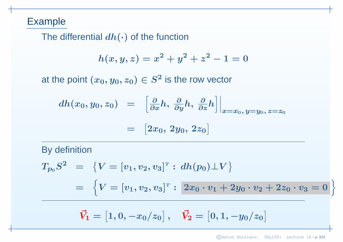
Example
The differential dh(·) of the function
h(x, y, z) = x2 + y2 + z2 − 1 = 0
at the point (x0, y0, z0) ∈ S2 is the row vector
dh(x0, y0, z0) =[
∂∂x
h, ∂∂y
h, ∂∂z
h]∣∣∣x=x0, y=y0, z=z0
=[2x0, 2y0, 2z0
]
By definition
Tp0S2 =
V = [v1, v2, v3]
T : dh(p0)⊥V
=
V = [v1, v2, v3]T : 2x0 · v1 + 2y0 · v2 + 2z0 · v3 = 0
~V1 =[1, 0, −x0/z0
], ~V2 =
[0, 1, −y0/z0
]
c©Anton Shiriaev. 5EL158: Lecture 16 – p. 3/21
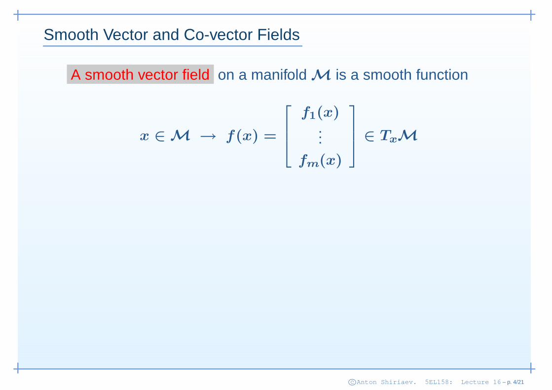
Smooth Vector and Co-vector Fields
A smooth vector field on a manifold M is a smooth function
x ∈ M → f(x) =
f1(x)...
fm(x)
∈ TxM
c©Anton Shiriaev. 5EL158: Lecture 16 – p. 4/21
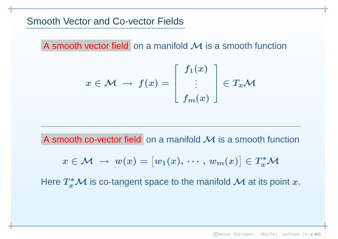
Smooth Vector and Co-vector Fields
A smooth vector field on a manifold M is a smooth function
x ∈ M → f(x) =
f1(x)...
fm(x)
∈ TxM
A smooth co-vector field on a manifold M is a smooth function
x ∈ M → w(x) =[w1(x), · · · , wm(x)
]∈ T ∗
xM
Here T ∗
xM is co-tangent space to the manifold M at its point x.
c©Anton Shiriaev. 5EL158: Lecture 16 – p. 4/21
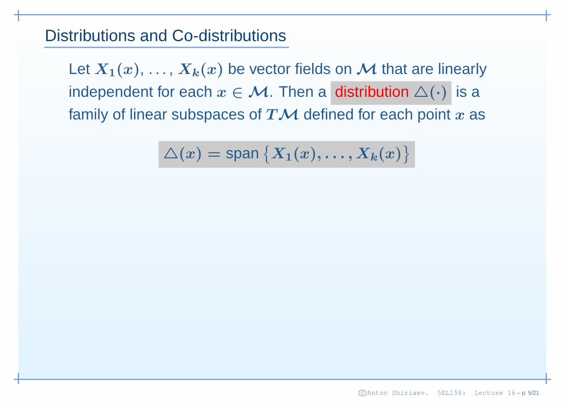
Distributions and Co-distributions
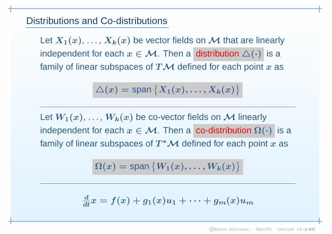
Let X1(x), . . . , Xk(x) be vector fields on M that are linearly
independent for each x ∈ M. Then a distribution (·) is a
family of linear subspaces of TM defined for each point x as
(x) = spanX1(x), . . . , Xk(x)
c©Anton Shiriaev. 5EL158: Lecture 16 – p. 5/21

Distributions and Co-distributions
Let X1(x), . . . , Xk(x) be vector fields on M that are linearly
independent for each x ∈ M. Then a distribution (·) is a
family of linear subspaces of TM defined for each point x as
(x) = spanX1(x), . . . , Xk(x)
Let W1(x), . . . , Wk(x) be co-vector fields on M linearly
independent for each x ∈ M. Then a co-distribution Ω(·) is a
family of linear subspaces of T ∗M defined for each point x as
Ω(x) = spanW1(x), . . . , Wk(x)
c©Anton Shiriaev. 5EL158: Lecture 16 – p. 5/21
Distributions and Co-distributions
Let X1(x), . . . , Xk(x) be vector fields on M that are linearly
independent for each x ∈ M. Then a distribution (·) is a
family of linear subspaces of TM defined for each point x as
(x) = spanX1(x), . . . , Xk(x)
Let W1(x), . . . , Wk(x) be co-vector fields on M linearly
independent for each x ∈ M. Then a co-distribution Ω(·) is a
family of linear subspaces of T ∗M defined for each point x as
Ω(x) = spanW1(x), . . . , Wk(x)
ddt
x = f(x) + g1(x)u1 + · · · + gm(x)um
c©Anton Shiriaev. 5EL158: Lecture 16 – p. 5/21
Lie Bracket of Vector Fields
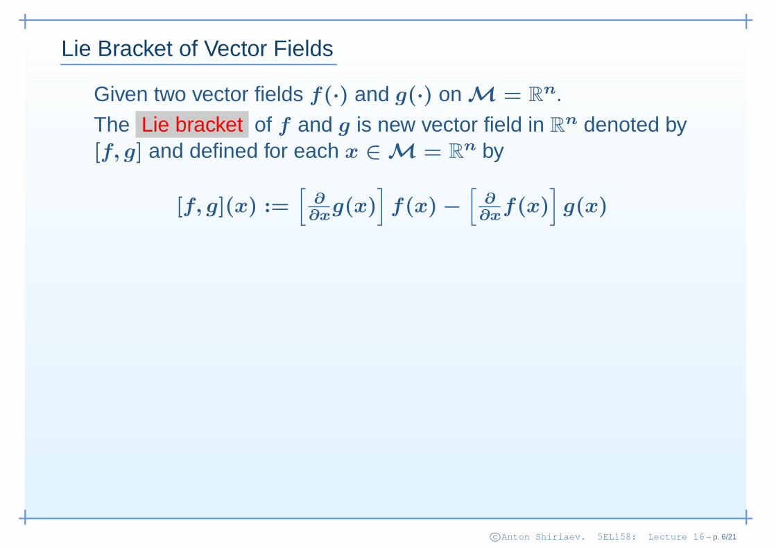
Given two vector fields f(·) and g(·) on M = Rn.
The Lie bracket of f and g is new vector field in Rn denoted by
[f, g] and defined for each x ∈ M = Rn by
[f, g](x) :=[
∂∂x
g(x)]
f(x) −[
∂∂x
f(x)]
g(x)
c©Anton Shiriaev. 5EL158: Lecture 16 – p. 6/21
Lie Bracket of Vector Fields
Given two vector fields f(·) and g(·) on M = Rn.
The Lie bracket of f and g is new vector field in Rn denoted by
[f, g] and defined for each x ∈ M = Rn by
[f, g](x) :=[
∂∂x
g(x)]
f(x) −[
∂∂x
f(x)]
g(x)
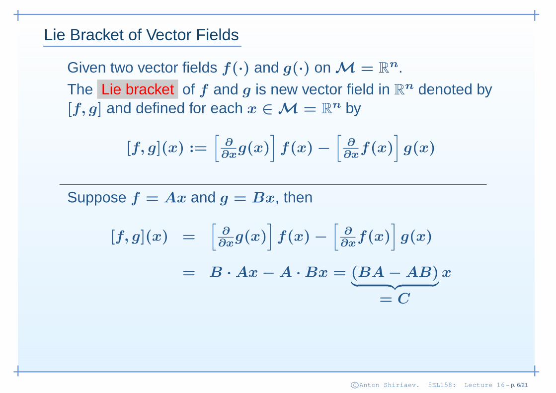
Suppose f = Ax and g = Bx, then
[f, g](x) =[
∂∂x
g(x)]
f(x) −[
∂∂x
f(x)]
g(x)
= B · Ax − A · Bx = (BA − AB)︸ ︷︷ ︸
= C
x
c©Anton Shiriaev. 5EL158: Lecture 16 – p. 6/21

Lie Bracket of Vector Fields
Given two vector fields f(·) and g(·) on M = Rn.
The Lie bracket of f and g is new vector field in Rn denoted by
[f, g] and defined for each x ∈ M = Rn by
[f, g](x) :=[
∂∂x
g(x)]
f(x) −[
∂∂x
f(x)]
g(x)
Notations:
ad0f(g) = g
ad1f(g) =
[f, g
]
ad2f(g) =
[f,
[f, g
] ]
...
adkf(g) =
[
f, ad(k−1)f (g)
]
c©Anton Shiriaev. 5EL158: Lecture 16 – p. 6/21
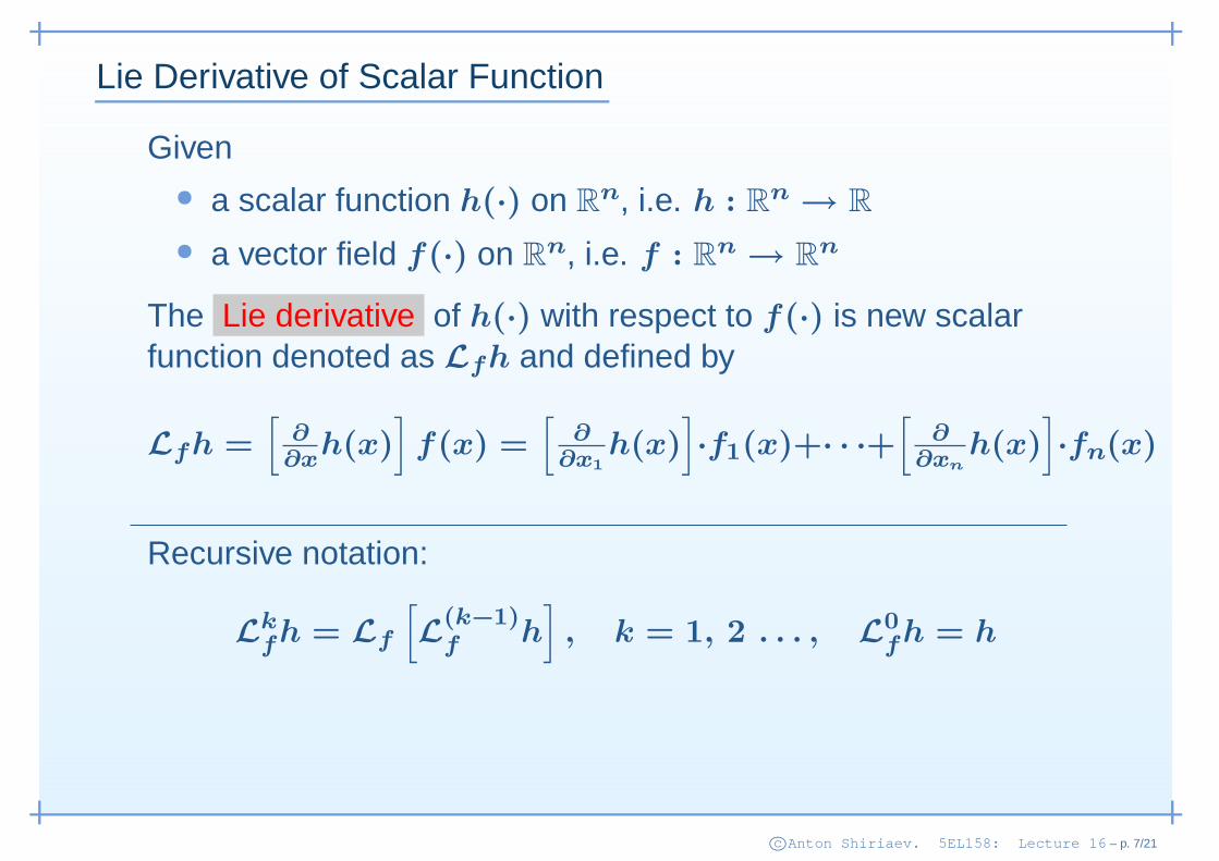
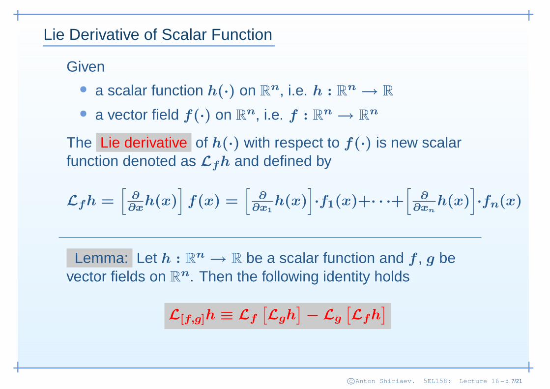
Lie Derivative of Scalar Function
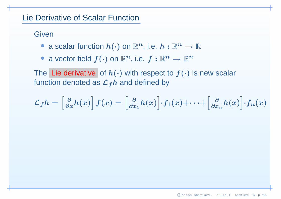
Given• a scalar function h(·) on R
n, i.e. h : Rn → R
• a vector field f(·) on Rn, i.e. f : R
n → Rn
The Lie derivative of h(·) with respect to f(·) is new scalarfunction denoted as Lfh and defined by
Lfh =[
∂∂x
h(x)]
f(x) =[
∂∂x1
h(x)]
·f1(x)+· · ·+[
∂∂xn
h(x)]
·fn(x)
c©Anton Shiriaev. 5EL158: Lecture 16 – p. 7/21
Lie Derivative of Scalar Function
Given• a scalar function h(·) on R
n, i.e. h : Rn → R
• a vector field f(·) on Rn, i.e. f : R
n → Rn
The Lie derivative of h(·) with respect to f(·) is new scalarfunction denoted as Lfh and defined by
Lfh =[
∂∂x
h(x)]
f(x) =[
∂∂x1
h(x)]
·f1(x)+· · ·+[
∂∂xn
h(x)]
·fn(x)
Recursive notation:
Lkfh = Lf
[
L(k−1)f h
]
, k = 1, 2 . . . , L0fh = h
c©Anton Shiriaev. 5EL158: Lecture 16 – p. 7/21
Lie Derivative of Scalar Function
Given• a scalar function h(·) on R
n, i.e. h : Rn → R
• a vector field f(·) on Rn, i.e. f : R
n → Rn
The Lie derivative of h(·) with respect to f(·) is new scalarfunction denoted as Lfh and defined by
Lfh =[
∂∂x
h(x)]
f(x) =[
∂∂x1
h(x)]
·f1(x)+· · ·+[
∂∂xn
h(x)]
·fn(x)
Lemma: Let h : Rn → R be a scalar function and f , g be
vector fields on Rn. Then the following identity holds
L[f,g]h ≡ Lf
[Lgh
]− Lg
[Lfh
]
c©Anton Shiriaev. 5EL158: Lecture 16 – p. 7/21

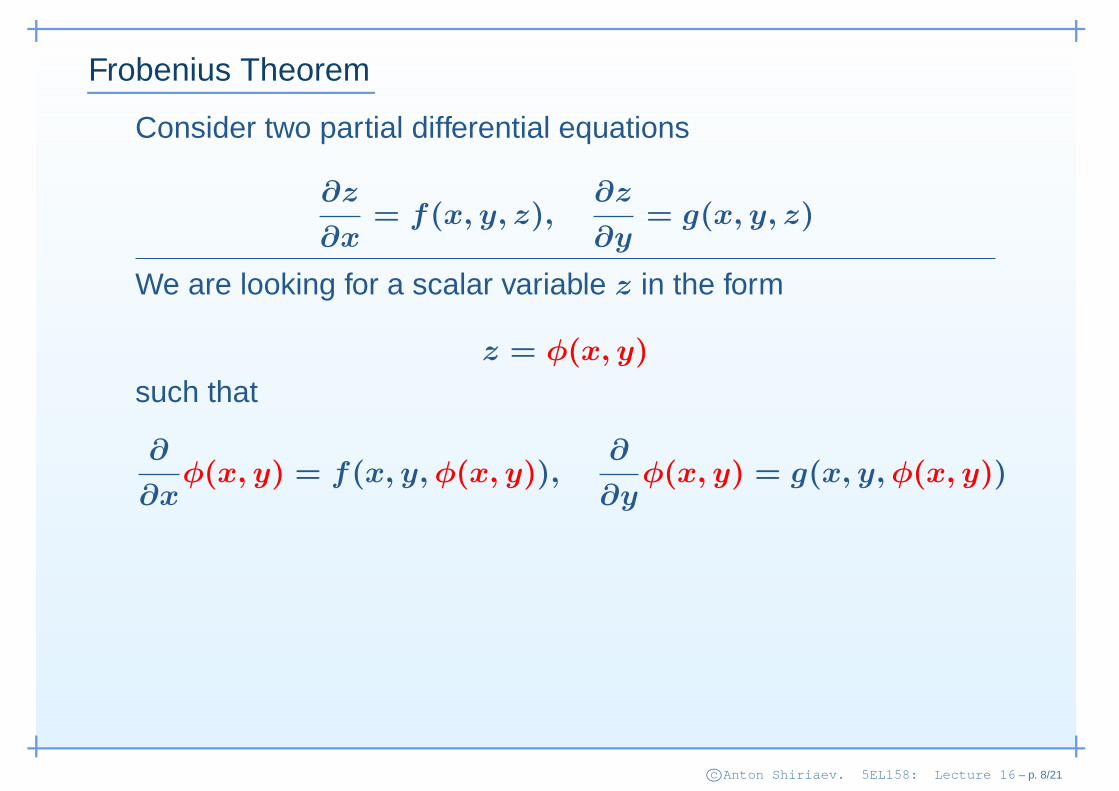
Frobenius Theorem
Consider two partial differential equations
∂z
∂x= f(x, y, z),
∂z
∂y= g(x, y, z)
c©Anton Shiriaev. 5EL158: Lecture 16 – p. 8/21
Frobenius Theorem
Consider two partial differential equations
∂z
∂x= f(x, y, z),
∂z
∂y= g(x, y, z)
We are looking for a scalar variable z in the form
z = φ(x, y)
such that
∂
∂xφ(x, y) = f(x, y, φ(x, y)),
∂
∂yφ(x, y) = g(x, y, φ(x, y))
c©Anton Shiriaev. 5EL158: Lecture 16 – p. 8/21

Frobenius Theorem
Consider two partial differential equations
∂z
∂x= f(x, y, z),
∂z
∂y= g(x, y, z)
We are looking for a scalar variable z in the form
z = φ(x, y)
such that
∂
∂xφ(x, y) = f(x, y, φ(x, y)),
∂
∂yφ(x, y) = g(x, y, φ(x, y))
If we find the solution, then it corresponds to the surface in R3
M =x, y, z = φ(x, y)
How to compute a tangent plane to that surface (manifold)?
c©Anton Shiriaev. 5EL158: Lecture 16 – p. 8/21
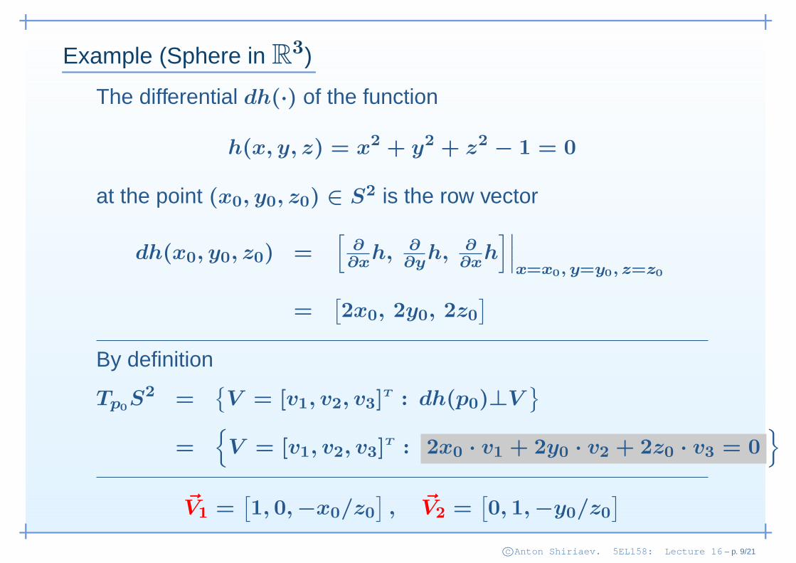
Example (Sphere in R3)
The differential dh(·) of the function
h(x, y, z) = x2 + y2 + z2 − 1 = 0
at the point (x0, y0, z0) ∈ S2 is the row vector
dh(x0, y0, z0) =[
∂∂x
h, ∂∂y
h, ∂∂x
h]∣∣∣x=x0, y=y0, z=z0
=[2x0, 2y0, 2z0
]
By definition
Tp0S2 =
V = [v1, v2, v3]
T : dh(p0)⊥V
=
V = [v1, v2, v3]T : 2x0 · v1 + 2y0 · v2 + 2z0 · v3 = 0
~V1 =[1, 0, −x0/z0
], ~V2 =
[0, 1, −y0/z0
]
c©Anton Shiriaev. 5EL158: Lecture 16 – p. 9/21
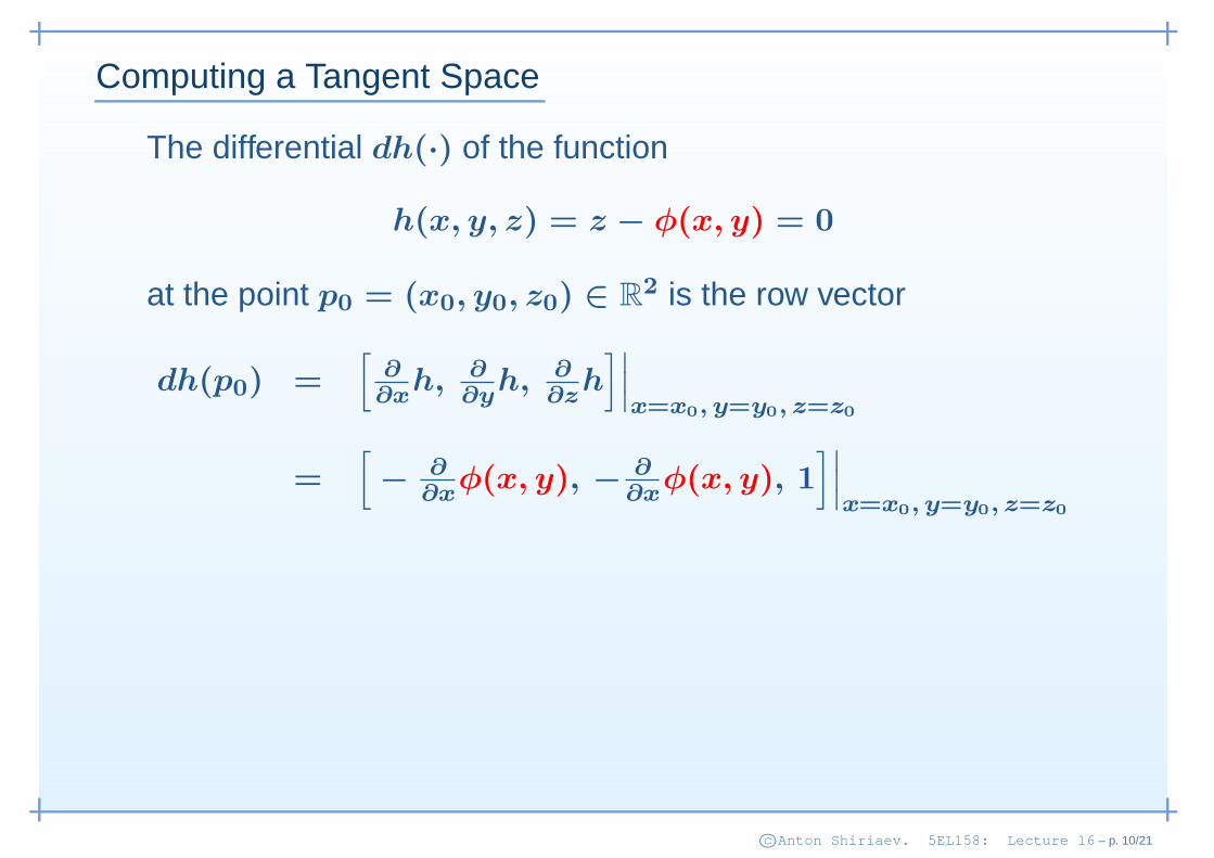
Computing a Tangent Space
The differential dh(·) of the function
h(x, y, z) = z − φ(x, y) = 0
at the point p0 = (x0, y0, z0) ∈ R2 is the row vector
dh(p0) =[
∂∂x
h, ∂∂y
h, ∂∂z
h]∣∣∣x=x0, y=y0, z=z0
=[
− ∂∂x
φ(x, y), − ∂∂x
φ(x, y), 1]∣∣∣x=x0, y=y0, z=z0
c©Anton Shiriaev. 5EL158: Lecture 16 – p. 10/21
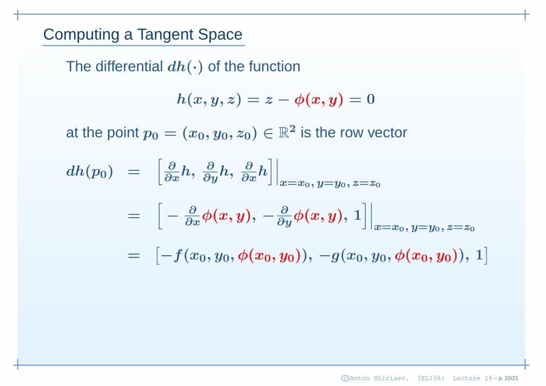
Computing a Tangent Space
The differential dh(·) of the function
h(x, y, z) = z − φ(x, y) = 0
at the point p0 = (x0, y0, z0) ∈ R2 is the row vector
dh(p0) =[
∂∂x
h, ∂∂y
h, ∂∂x
h]∣∣∣x=x0, y=y0, z=z0
=[
− ∂∂x
φ(x, y), − ∂∂y
φ(x, y), 1]∣∣∣x=x0, y=y0, z=z0
=[−f(x0, y0, φ(x0, y0)), −g(x0, y0, φ(x0, y0)), 1
]
c©Anton Shiriaev. 5EL158: Lecture 16 – p. 10/21

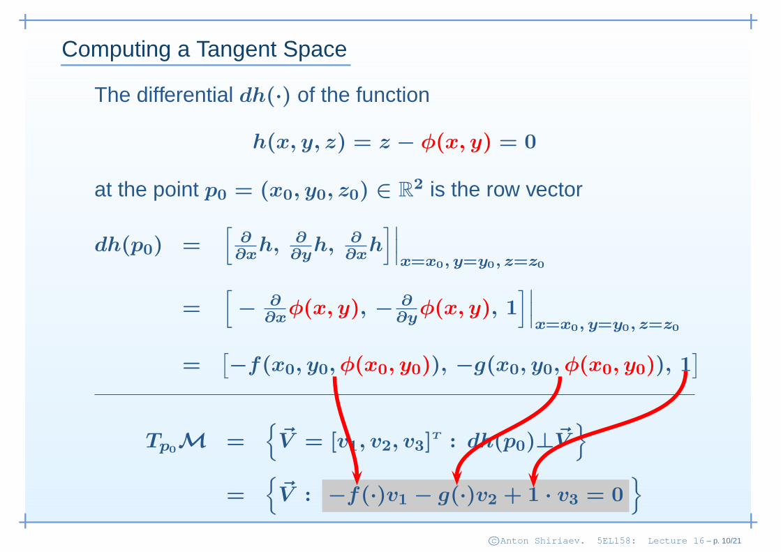
Computing a Tangent Space
The differential dh(·) of the function
h(x, y, z) = z − φ(x, y) = 0
at the point p0 = (x0, y0, z0) ∈ R2 is the row vector
dh(p0) =[
∂∂x
h, ∂∂y
h, ∂∂x
h]∣∣∣x=x0, y=y0, z=z0
=[
− ∂∂x
φ(x, y), − ∂∂y
φ(x, y), 1]∣∣∣x=x0, y=y0, z=z0
=[−f(x0, y0, φ(x0, y0)), −g(x0, y0, φ(x0, y0)), 1
]
Tp0M =
~V = [v1, v2, v3]T : dh(p0)⊥~V
=
~V : −f(·)v1 − g(·)v2 + 1 · v3 = 0
c©Anton Shiriaev. 5EL158: Lecture 16 – p. 10/21
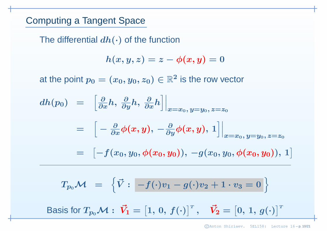
Computing a Tangent Space
The differential dh(·) of the function
h(x, y, z) = z − φ(x, y) = 0
at the point p0 = (x0, y0, z0) ∈ R2 is the row vector
dh(p0) =[
∂∂x
h, ∂∂y
h, ∂∂x
h]∣∣∣x=x0, y=y0, z=z0
=[
− ∂∂x
φ(x, y), − ∂∂y
φ(x, y), 1]∣∣∣x=x0, y=y0, z=z0
=[−f(x0, y0, φ(x0, y0)), −g(x0, y0, φ(x0, y0)), 1
]
Tp0M =
~V : −f(·)v1 − g(·)v2 + 1 · v3 = 0
Basis for Tp0M : ~V1 =
[1, 0, f(·)
]T
, ~V2 =[0, 1, g(·)
]T
c©Anton Shiriaev. 5EL158: Lecture 16 – p. 10/21
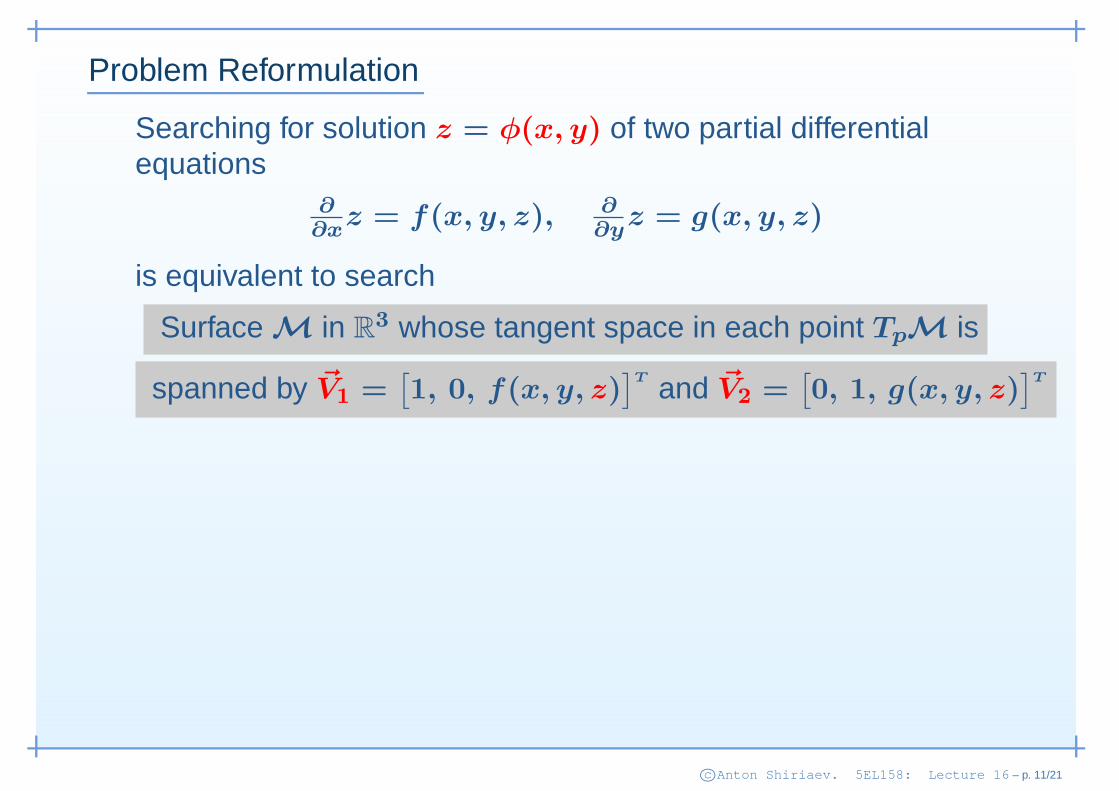
Problem Reformulation
Searching for solution z = φ(x, y) of two partial differentialequations
∂∂x
z = f(x, y, z), ∂∂y
z = g(x, y, z)
is equivalent to search
Surface M in R3 whose tangent space in each point TpM is
spanned by ~V1 =[1, 0, f(x, y, z)
]T and ~V2 =
[0, 1, g(x, y, z)
]T
c©Anton Shiriaev. 5EL158: Lecture 16 – p. 11/21
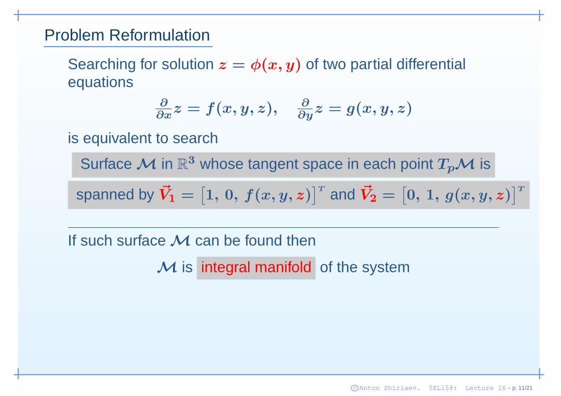
Problem Reformulation
Searching for solution z = φ(x, y) of two partial differentialequations
∂∂x
z = f(x, y, z), ∂∂y
z = g(x, y, z)
is equivalent to search
Surface M in R3 whose tangent space in each point TpM is
spanned by ~V1 =[1, 0, f(x, y, z)
]T and ~V2 =
[0, 1, g(x, y, z)
]T
If such surface M can be found then
M is integral manifold of the system
c©Anton Shiriaev. 5EL158: Lecture 16 – p. 11/21
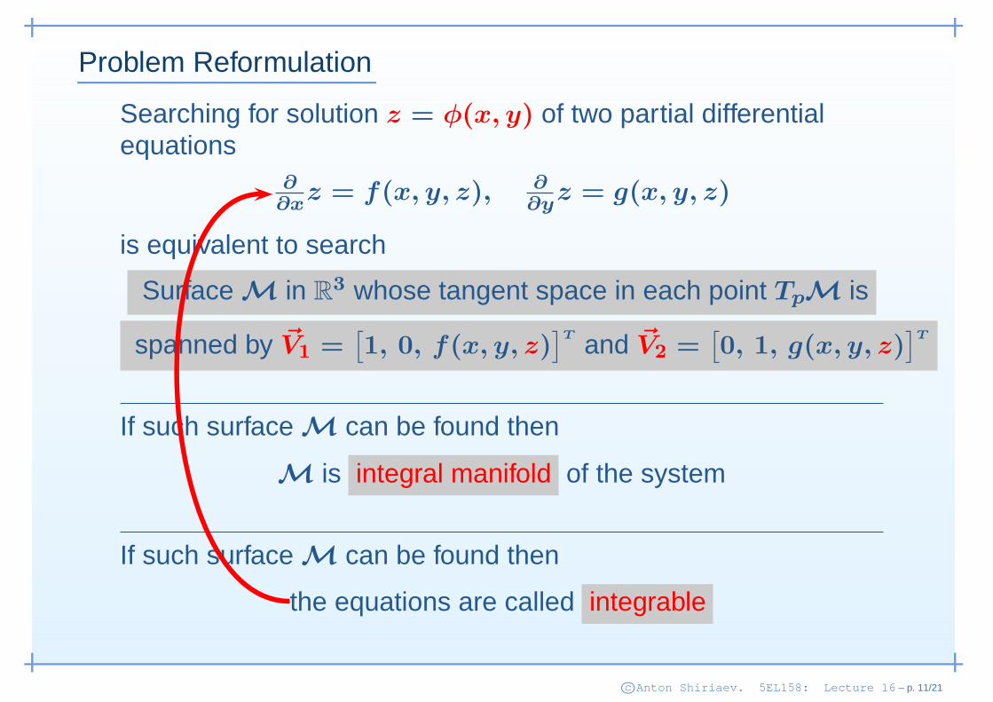
Problem Reformulation
Searching for solution z = φ(x, y) of two partial differentialequations
∂∂x
z = f(x, y, z), ∂∂y
z = g(x, y, z)
is equivalent to search
Surface M in R3 whose tangent space in each point TpM is
spanned by ~V1 =[1, 0, f(x, y, z)
]T and ~V2 =
[0, 1, g(x, y, z)
]T
If such surface M can be found then
M is integral manifold of the system
If such surface M can be found then
the equations are called integrable
c©Anton Shiriaev. 5EL158: Lecture 16 – p. 11/21
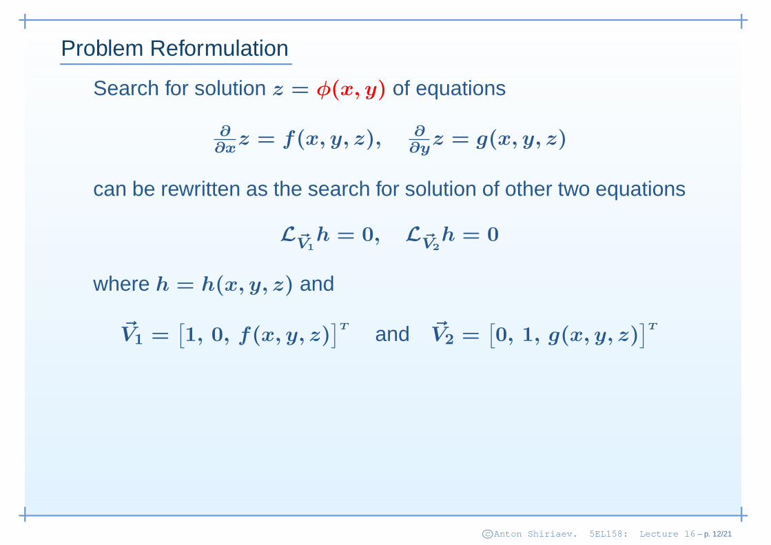
Problem Reformulation
Search for solution z = φ(x, y) of equations
∂∂x
z = f(x, y, z), ∂∂y
z = g(x, y, z)
can be rewritten as the search for solution of other two equations
L~V1
h = 0, L~V2
h = 0
where h = h(x, y, z) and
~V1 =[1, 0, f(x, y, z)
]T and ~V2 =
[0, 1, g(x, y, z)
]T
c©Anton Shiriaev. 5EL158: Lecture 16 – p. 12/21
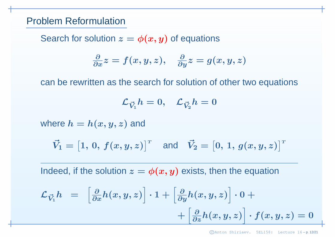
Problem Reformulation
Search for solution z = φ(x, y) of equations
∂∂x
z = f(x, y, z), ∂∂y
z = g(x, y, z)
can be rewritten as the search for solution of other two equations
L~V1
h = 0, L~V2
h = 0
where h = h(x, y, z) and
~V1 =[1, 0, f(x, y, z)
]T and ~V2 =
[0, 1, g(x, y, z)
]T
Indeed, if the solution z = φ(x, y) exists, then the equation
L~V1
h =[
∂∂x
h(x, y, z)]
· 1 +[
∂∂y
h(x, y, z)]
· 0 +
+[
∂∂z
h(x, y, z)]
· f(x, y, z) = 0
c©Anton Shiriaev. 5EL158: Lecture 16 – p. 12/21
Problem Reformulation
Search for solution z = φ(x, y) of equations
∂∂x
z = f(x, y, z), ∂∂y
z = g(x, y, z)
can be rewritten as the search for solution of other two equations
L~V1
h = 0, L~V2
h = 0
where h = h(x, y, z) and
~V1 =[1, 0, f(x, y, z)
]T and ~V2 =
[0, 1, g(x, y, z)
]T
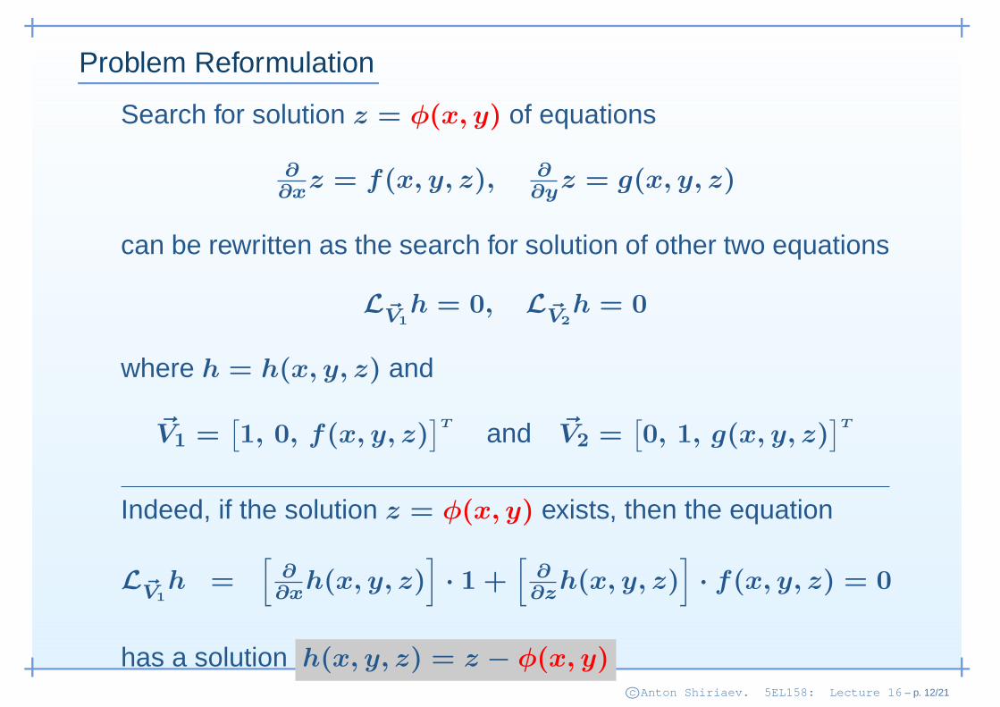
Indeed, if the solution z = φ(x, y) exists, then the equation
L~V1
h =[
∂∂x
h(x, y, z)]
· 1 +[
∂∂z
h(x, y, z)]
· f(x, y, z) = 0
has a solution h(x, y, z) = z − φ(x, y)c©Anton Shiriaev. 5EL158: Lecture 16 – p. 12/21
Problem Reformulation
Search for solution z = φ(x, y) of equations
∂∂x
z = f(x, y, z), ∂∂y
z = g(x, y, z)
can be rewritten as the search for solution of other two equations
L~V1
h = 0, L~V2
h = 0
where h = h(x, y, z) and
~V1 =[1, 0, f(x, y, z)
]T and ~V2 =
[0, 1, g(x, y, z)
]T
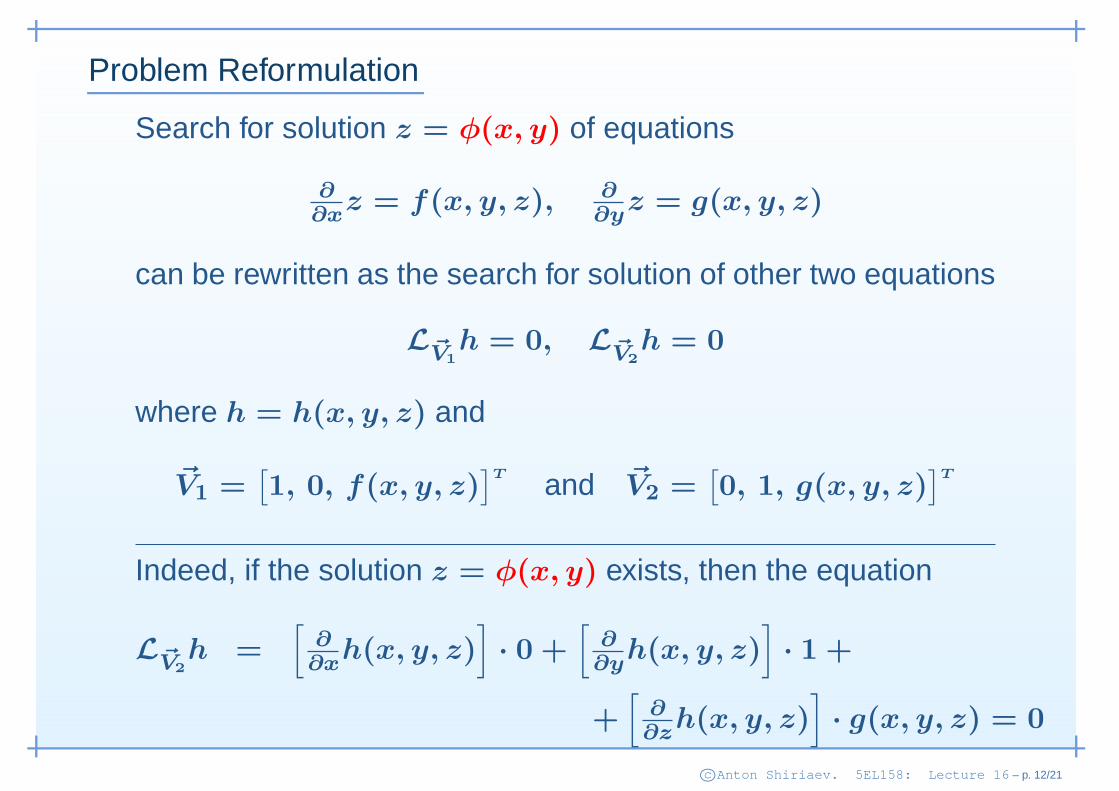
Indeed, if the solution z = φ(x, y) exists, then the equation
L~V2
h =[
∂∂x
h(x, y, z)]
· 0 +[
∂∂y
h(x, y, z)]
· 1 +
+[
∂∂z
h(x, y, z)]
· g(x, y, z) = 0
c©Anton Shiriaev. 5EL158: Lecture 16 – p. 12/21

Problem Reformulation
Search for solution z = φ(x, y) of equations
∂∂x
z = f(x, y, z), ∂∂y
z = g(x, y, z)
can be rewritten as the search for solution of other two equations
L~V1
h = 0, L~V2
h = 0
where h = h(x, y, z) and
~V1 =[1, 0, f(x, y, z)
]T and ~V2 =
[0, 1, g(x, y, z)
]T
Indeed, if the solution z = φ(x, y) exists, then the equation
L~V2
h =[
∂∂y
h(x, y, z)]
· 1 +[
∂∂z
h(x, y, z)]
· g(x, y, z) = 0
has a solution h(x, y, z) = z − φ(x, y)c©Anton Shiriaev. 5EL158: Lecture 16 – p. 12/21
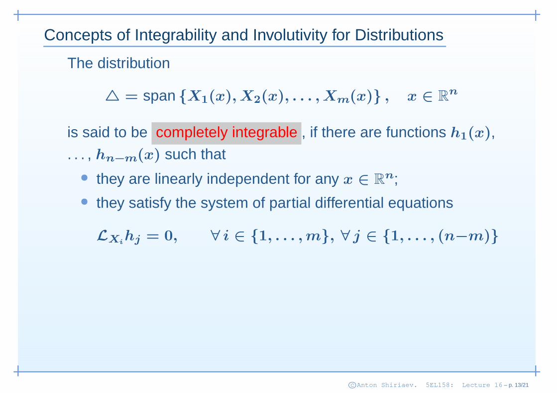
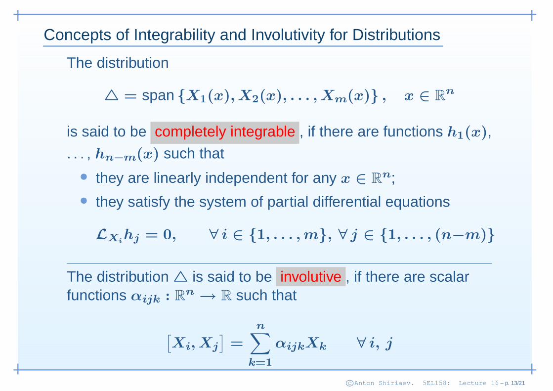
Concepts of Integrability and Involutivity for Distributions
The distribution
= span X1(x), X2(x), . . . , Xm(x) , x ∈ Rn
is said to be completely integrable , if there are functions h1(x),
. . . , hn−m(x) such that
• they are linearly independent for any x ∈ Rn;
• they satisfy the system of partial differential equations
LXihj = 0, ∀ i ∈ 1, . . . , m, ∀ j ∈ 1, . . . , (n−m)
c©Anton Shiriaev. 5EL158: Lecture 16 – p. 13/21
Concepts of Integrability and Involutivity for Distributions
The distribution
= span X1(x), X2(x), . . . , Xm(x) , x ∈ Rn
is said to be completely integrable , if there are functions h1(x),
. . . , hn−m(x) such that
• they are linearly independent for any x ∈ Rn;
• they satisfy the system of partial differential equations
LXihj = 0, ∀ i ∈ 1, . . . , m, ∀ j ∈ 1, . . . , (n−m)
The distribution is said to be involutive , if there are scalarfunctions αijk : R
n → R such that
[Xi, Xj
]=
n∑
k=1
αijkXk ∀ i, j
c©Anton Shiriaev. 5EL158: Lecture 16 – p. 13/21
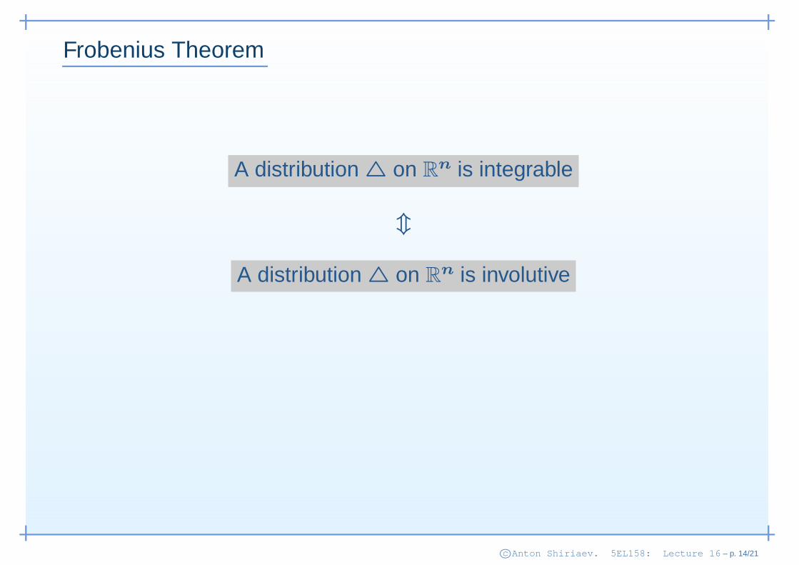
Frobenius Theorem
A distribution on Rn is integrable
m
A distribution on Rn is involutive
c©Anton Shiriaev. 5EL158: Lecture 16 – p. 14/21
Lecture 16: Geometric Nonlinear Control
• Background and Useful Concepts
• Feedback Linearization
• Feedback Linearization for Single Link Flexible Joint
c©Anton Shiriaev. 5EL158: Lecture 16 – p. 15/21
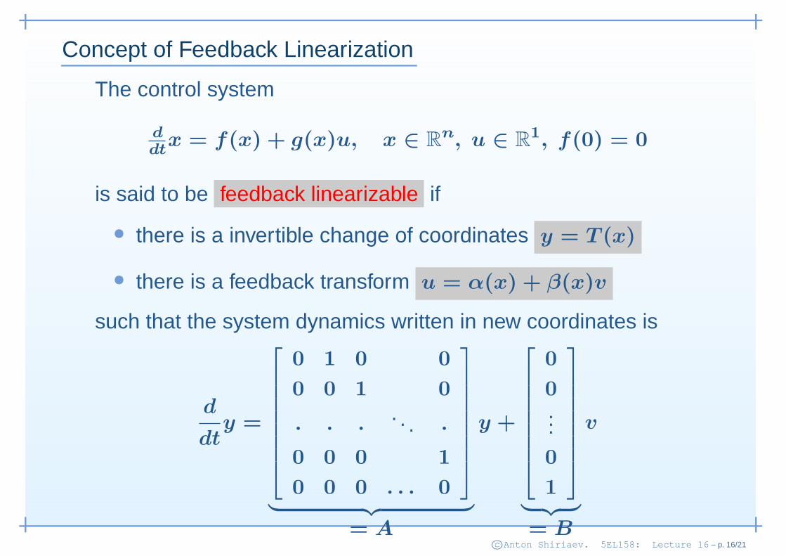
Concept of Feedback Linearization
The control system
ddt
x = f(x) + g(x)u, x ∈ Rn, u ∈ R
1, f(0) = 0
is said to be feedback linearizable if
• there is a invertible change of coordinates y = T (x)
• there is a feedback transform u = α(x) + β(x)v
such that the system dynamics written in new coordinates is
d
dty =
0 1 0 0
0 0 1 0
· · ·. . . ·
0 0 0 1
0 0 0 . . . 0
︸ ︷︷ ︸
= A
y +
0
0...0
1
︸ ︷︷ ︸
= B
v
c©Anton Shiriaev. 5EL158: Lecture 16 – p. 16/21
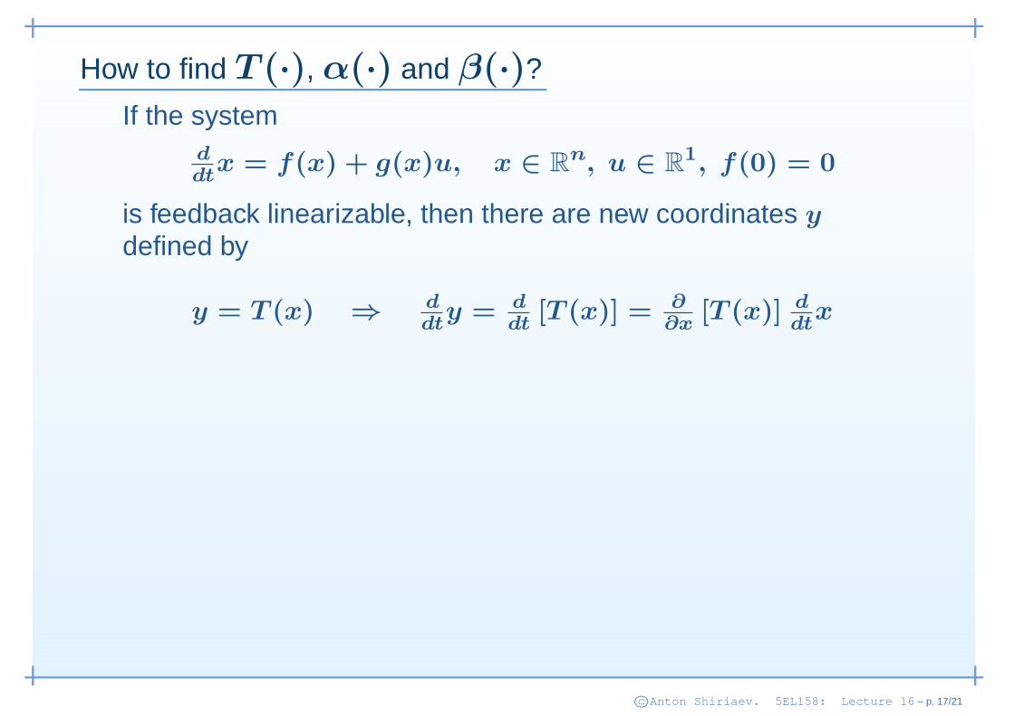
How to find T (·), α(·) and β(·)?
If the systemddt
x = f(x) + g(x)u, x ∈ Rn, u ∈ R
1, f(0) = 0
is feedback linearizable, then there are new coordinates ydefined by
y = T (x) ⇒ ddt
y = ddt
[T (x)] = ∂∂x
[T (x)] ddt
x
c©Anton Shiriaev. 5EL158: Lecture 16 – p. 17/21
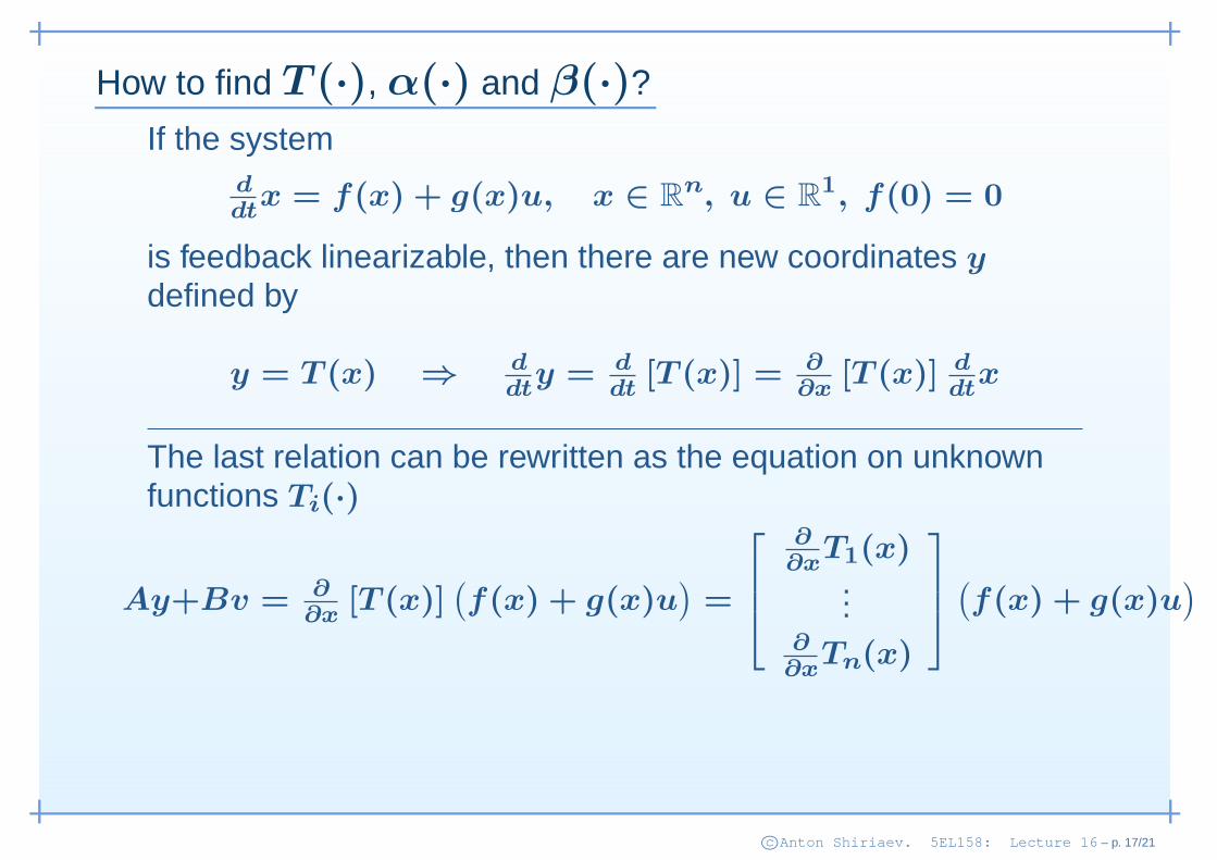
How to find T (·), α(·) and β(·)?
If the systemddt
x = f(x) + g(x)u, x ∈ Rn, u ∈ R
1, f(0) = 0
is feedback linearizable, then there are new coordinates ydefined by
y = T (x) ⇒ ddt
y = ddt
[T (x)] = ∂∂x
[T (x)] ddt
x
The last relation can be rewritten as the equation on unknownfunctions Ti(·)
Ay+Bv = ∂∂x
[T (x)](f(x) + g(x)u
)=
∂∂x
T1(x)...
∂∂x
Tn(x)
(f(x) + g(x)u
)
c©Anton Shiriaev. 5EL158: Lecture 16 – p. 17/21
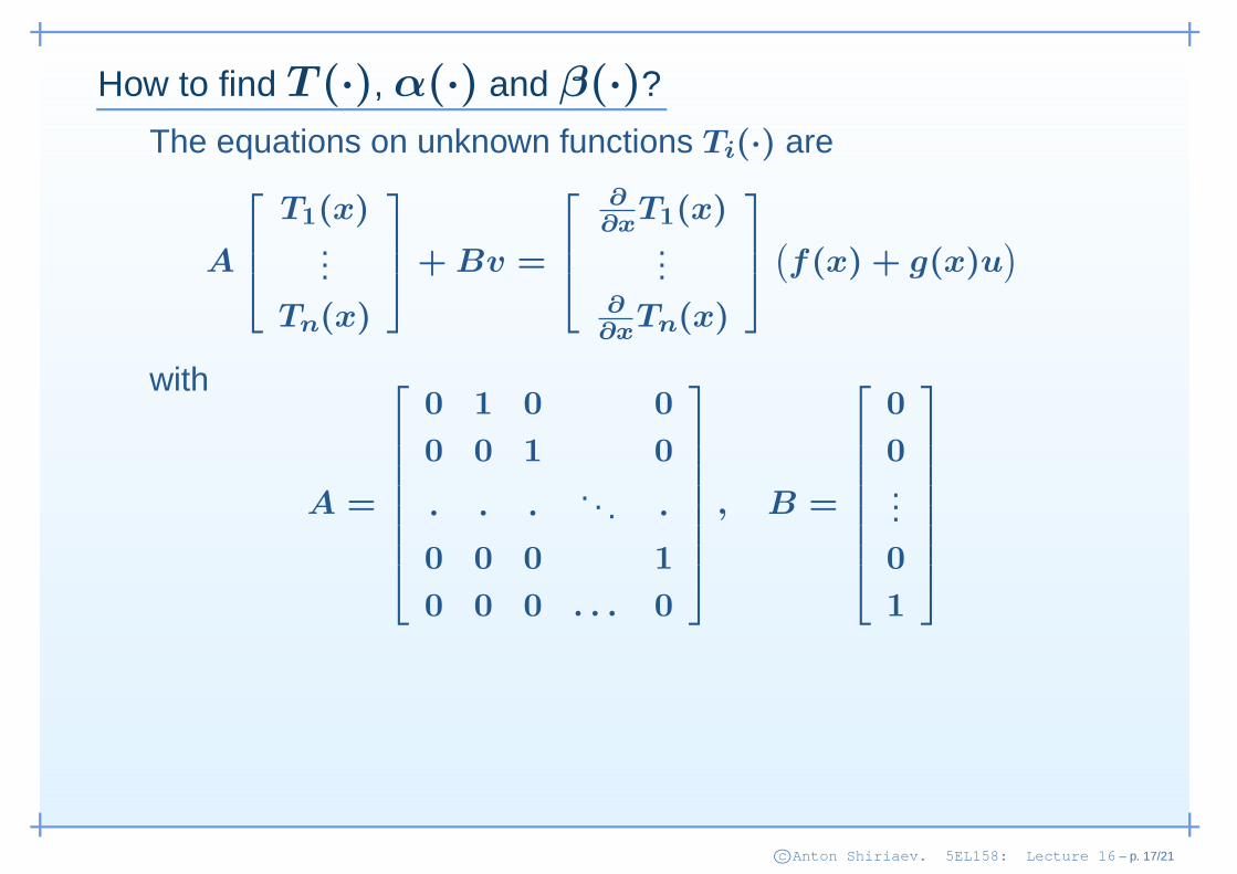
How to find T (·), α(·) and β(·)?
The equations on unknown functions Ti(·) are
A
T1(x)...
Tn(x)
+ Bv =
∂∂x
T1(x)...
∂∂x
Tn(x)
(f(x) + g(x)u
)
with
A =
0 1 0 0
0 0 1 0
· · ·. . . ·
0 0 0 1
0 0 0 . . . 0
, B =
0
0...0
1
c©Anton Shiriaev. 5EL158: Lecture 16 – p. 17/21
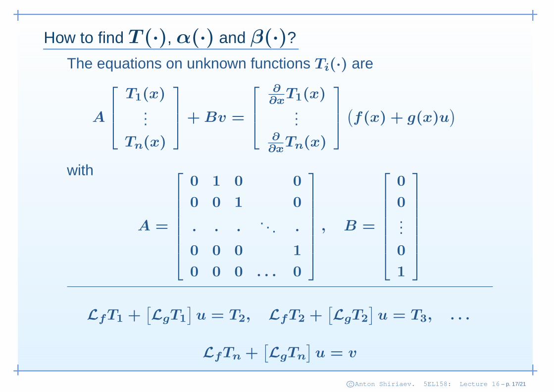
How to find T (·), α(·) and β(·)?
The equations on unknown functions Ti(·) are
A
T1(x)...
Tn(x)
+ Bv =
∂∂x
T1(x)...
∂∂x
Tn(x)
(f(x) + g(x)u
)
with
A =
0 1 0 0
0 0 1 0
· · ·. . . ·
0 0 0 1
0 0 0 . . . 0
, B =
0
0...0
1
LfT1 +[LgT1
]u = T2, LfT2 +
[LgT2
]u = T3, . . .
LfTn +[LgTn
]u = v
c©Anton Shiriaev. 5EL158: Lecture 16 – p. 17/21
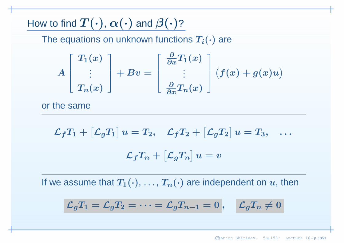
How to find T (·), α(·) and β(·)?
The equations on unknown functions Ti(·) are
A
T1(x)...
Tn(x)
+ Bv =
∂∂x
T1(x)...
∂∂x
Tn(x)
(f(x) + g(x)u
)
or the same
LfT1 +[LgT1
]u = T2, LfT2 +
[LgT2
]u = T3, . . .
LfTn +[LgTn
]u = v
If we assume that T1(·), . . . , Tn(·) are independent on u, then
LgT1 = LgT2 = · · · = LgTn−1 = 0 , LgTn 6= 0
c©Anton Shiriaev. 5EL158: Lecture 16 – p. 18/21
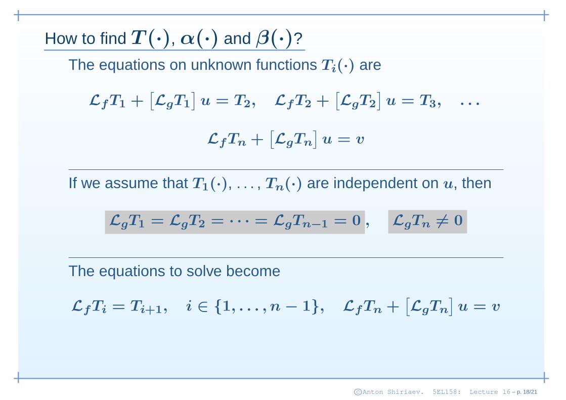
How to find T (·), α(·) and β(·)?
The equations on unknown functions Ti(·) are
LfT1 +[LgT1
]u = T2, LfT2 +
[LgT2
]u = T3, . . .
LfTn +[LgTn
]u = v
If we assume that T1(·), . . . , Tn(·) are independent on u, then
LgT1 = LgT2 = · · · = LgTn−1 = 0 , LgTn 6= 0
The equations to solve become
LfTi = Ti+1, i ∈ 1, . . . , n − 1, LfTn +[LgTn
]u = v
c©Anton Shiriaev. 5EL158: Lecture 16 – p. 18/21
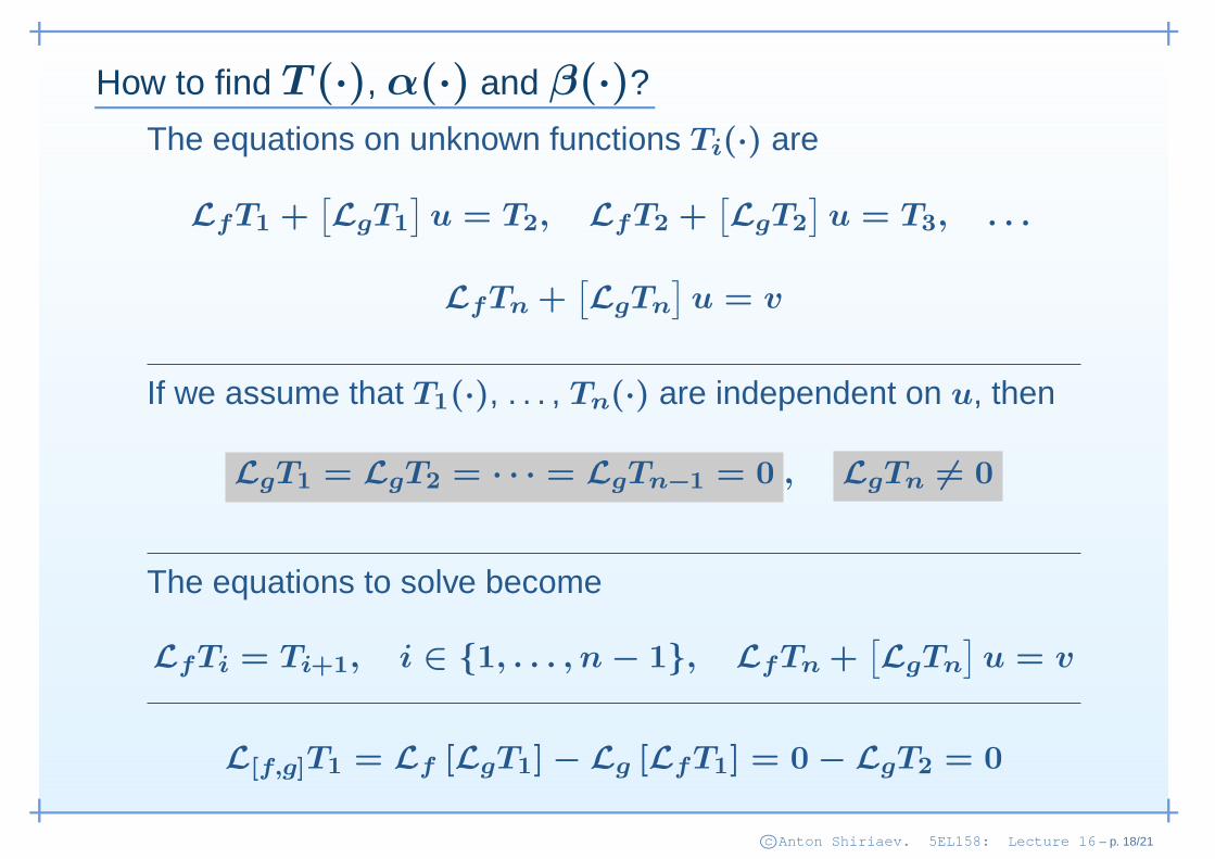
How to find T (·), α(·) and β(·)?
The equations on unknown functions Ti(·) are
LfT1 +[LgT1
]u = T2, LfT2 +
[LgT2
]u = T3, . . .
LfTn +[LgTn
]u = v
If we assume that T1(·), . . . , Tn(·) are independent on u, then
LgT1 = LgT2 = · · · = LgTn−1 = 0 , LgTn 6= 0
The equations to solve become
LfTi = Ti+1, i ∈ 1, . . . , n − 1, LfTn +[LgTn
]u = v
L[f,g]T1 = Lf [LgT1] − Lg [LfT1] = 0 − LgT2 = 0
c©Anton Shiriaev. 5EL158: Lecture 16 – p. 18/21
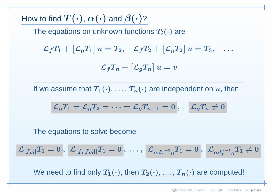
How to find T (·), α(·) and β(·)?
The equations on unknown functions Ti(·) are
LfT1 +[LgT1
]u = T2, LfT2 +
[LgT2
]u = T3, . . .
LfTn +[LgTn
]u = v
If we assume that T1(·), . . . , Tn(·) are independent on u, then
LgT1 = LgT2 = · · · = LgTn−1 = 0 , LgTn 6= 0
The equations to solve become
L[f,g]T1 = 0 , L[f,[f,g]]T1 = 0 , . . . , Lad
n−2
f gT1 = 0 , L
adn−1
f gT1 6= 0
We need to find only T1(·), then T2(·), . . . , Tn(·) are computed!
c©Anton Shiriaev. 5EL158: Lecture 16 – p. 18/21
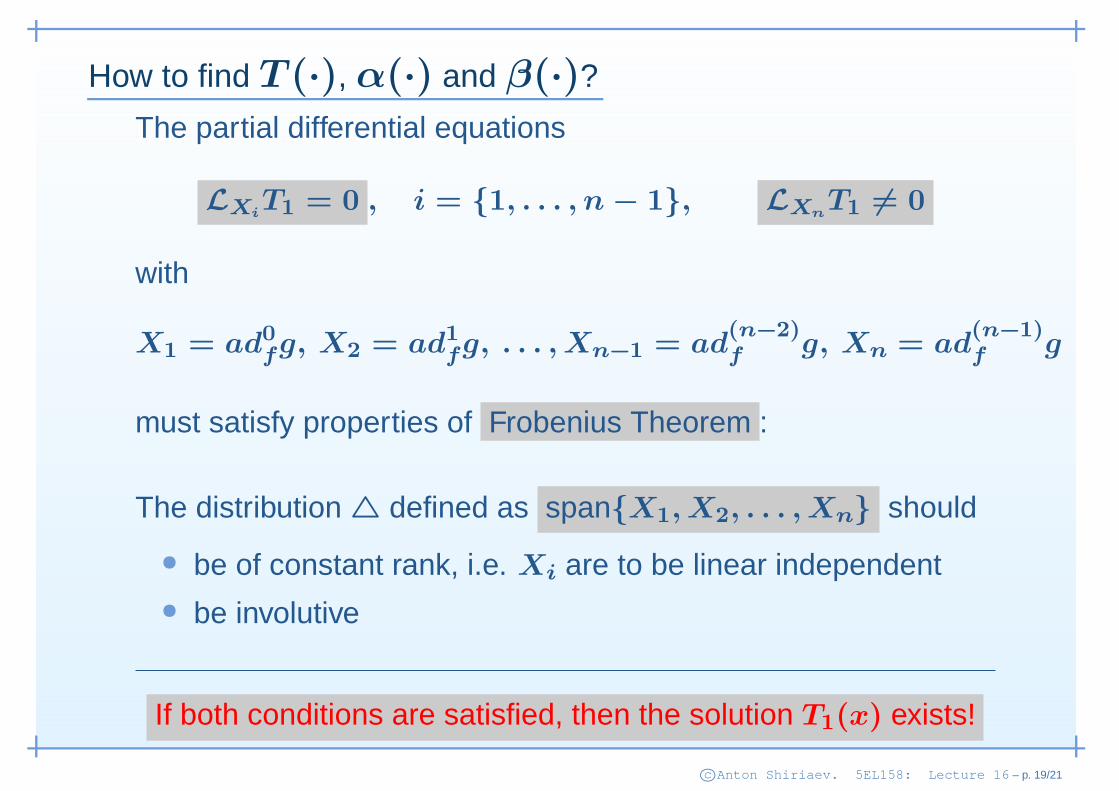
How to find T (·), α(·) and β(·)?
The partial differential equations
LXiT1 = 0 , i = 1, . . . , n − 1, LXn
T1 6= 0
with
X1 = ad0fg, X2 = ad1
fg, . . . , Xn−1 = ad(n−2)f g, Xn = ad
(n−1)f g
must satisfy properties of Frobenius Theorem :
The distribution defined as spanX1, X2, . . . , Xn should
• be of constant rank, i.e. Xi are to be linear independent• be involutive
If both conditions are satisfied, then the solution T1(x) exists!
c©Anton Shiriaev. 5EL158: Lecture 16 – p. 19/21
Lecture 16: Geometric Nonlinear Control
• Background and Useful Concepts
• Feedback Linearization
• Feedback Linearization for Single Link Flexible Joint
c©Anton Shiriaev. 5EL158: Lecture 16 – p. 20/21
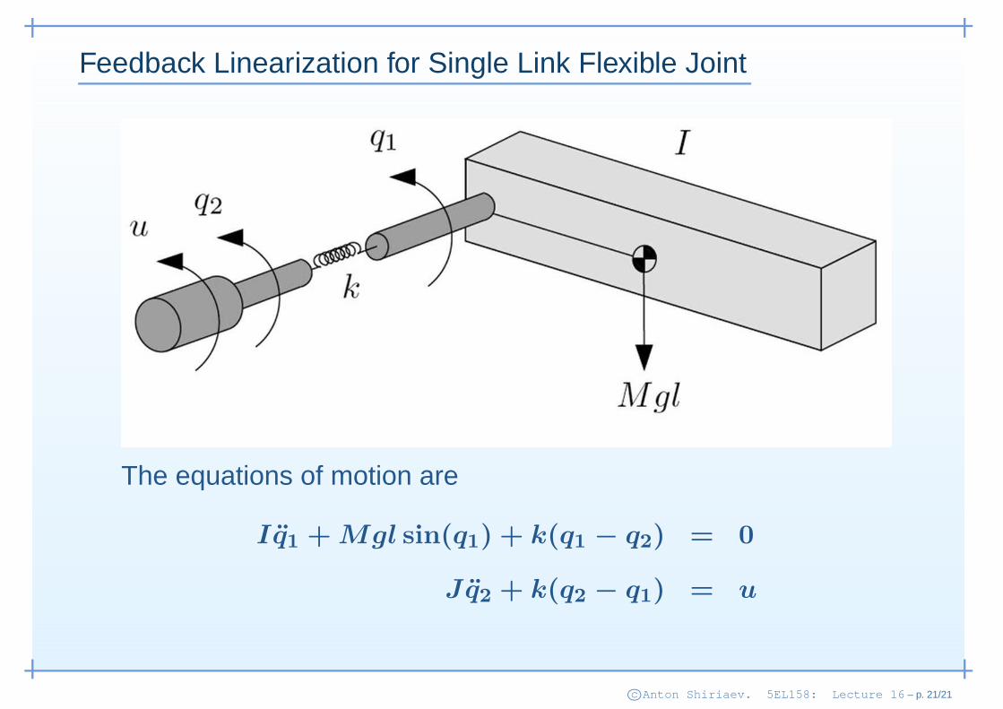
Feedback Linearization for Single Link Flexible Joint
The equations of motion are
Iq1 + Mgl sin(q1) + k(q1 − q2) = 0
Jq2 + k(q2 − q1) = u
c©Anton Shiriaev. 5EL158: Lecture 16 – p. 21/21
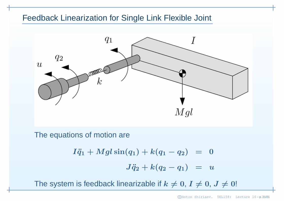
Feedback Linearization for Single Link Flexible Joint
The equations of motion are
Iq1 + Mgl sin(q1) + k(q1 − q2) = 0
Jq2 + k(q2 − q1) = u
The system is feedback linearizable if k 6= 0, I 6= 0, J 6= 0!
c©Anton Shiriaev. 5EL158: Lecture 16 – p. 21/21