lecture 16: polynomial and categorical regressioncshalizi/mreg/15/lectures/lecture-16.pdflecture 16:...

23:46 Saturday 24th October, 2015See updates and corrections at http://www.stat.cmu.edu/~cshalizi/mreg/

Lecture 16: Polynomial and Categorical

Regression

36-401, Fall 2015, Section B

22 October 2015

Contents

1 Essentials of Multiple Linear Regression 1

2 Adding Curvature: Polynomial Regression 22.1 R Practicalities . . . . . . . . . . . . . . . . . . . . . . . . . . . . 32.2 Properties, Issues, and Caveats . . . . . . . . . . . . . . . . . . . 62.3 Orthogonal Polynomials . . . . . . . . . . . . . . . . . . . . . . . 82.4 Non-Polynomial Function Bases . . . . . . . . . . . . . . . . . . . 9

3 Categorical Predictors 113.1 Binary Categories . . . . . . . . . . . . . . . . . . . . . . . . . . . 11

3.1.1 “Adjusted effect of a category” . . . . . . . . . . . . . . . 133.2 Categorical Variables with More than Two Levels . . . . . . . . . 143.3 Two, Three, Many Categorical Predictors . . . . . . . . . . . . . 153.4 Analysis of Variance: Only Categorical Predictors . . . . . . . . 153.5 Ordinal Variables . . . . . . . . . . . . . . . . . . . . . . . . . . . 163.6 Detailed R Example . . . . . . . . . . . . . . . . . . . . . . . . . 16

4 Further Reading 23

5 Exercises 24

1 Essentials of Multiple Linear Regression

We predict a scalar random variable Y as a linear function of p different predictorvariables X1, . . . Xp, plus noise:

Y = β0 + β1X1 + . . . βpXp + ε

and assume that E [ε|X] = 0, Var [ε|X] = σ2, with ε being uncorrelated acrossobservations. In matrix form,

Y = Xβ + ε

1

http://www.stat.cmu.edu/~cshalizi/mreg/

2

the design matrix X including an extra column of 1s to handle the intercept,and E [ε|X] = 0, Var [ε|X] = σ2I.

If we add the Gaussian noise assumption, ε ∼ MVN(0, σ2I), independentof all the predictor variables.

The least squares estimate of the coefficient vector, which is also the maxi-mum likelihood estimate if the noise is Gaussian, is

β = (xTx)−1xTy

These are unbiased, with variance σ2(xTx)−1. Under the Gaussian noise as-

sumption, β itself has a Gaussian distribution. The standard error se[βi

]=

σ√

(xTx)−1ii . Fitted values are given by xβ = Hy, and residuals by e =

(I−H)y. Fitted values m and residuals e are also unbiased and have Gaussiandistributions, with variance matrices σ2H and σ2(I−H), respectively.

When (as is usually the case) σ2 is unknown, the maximum likelihood es-timator is the in-sample mean-squared error, n−1(eTe) is a negatively biasedestimator of σ2: E

[σ2]

= σ2 n−p−1n . Under the Gaussian noise assumption,

nσ2/σ2 ∼ χ2n−p−1. Also under the Gaussian noise assumption, the Gaussian

sampling distribution of any particular coefficient or conditional mean can beconverted into a t distribution, with n− p− 1 degrees of freedom, by using theappropriate standard error, obtained by plugging in the de-biased estimate ofσ2.

None of these results require any assumptions on the predictor variablesXi, except that they take real numerical values, and that they are linearlyindependent.

2 Adding Curvature: Polynomial Regression

Because the predictor variables are almost totally arbitrary, there is no harm inmaking one predictor variable a function of another, so long as it isn’t a linearfunction. In particular, there is nothing wrong with a model like

Y = β0 + β1X1 + β2X21 + . . . βdX

d1 + βd+1X2 + . . . βp+d−1Xp + ε

where instead of Y being linearly related to X1, it’s polynomially related, withthe order of the polynomial being d. We just add d − 1 columns to the designmatrix x, containing x21, x

31, . . . x

d1, and treat them just as we would any other

predictor variables. With this expanded design matrix, it’s still true that x =(xTx)−1xTy, that fitted values are Hy (using the expanded x to get H), etc.The number of degrees of freedom for the residuals will be n− (p+ 1 + (d− 1)).

Nor is there principled reason why every predictor variable can’t have its ownpolynomial, each with (potentially) a different degree di. In that case, number-ing the βs sequentially gets tricky, and better notation would be somethinglike

Y = β0 +

p∑i=1

di∑j=1

βi,jXji + ε

23:46 Saturday 24th October, 2015

3 2.1 R Practicalities

though then we’d have to remember to “stack” the βi,js into a vector of length1 +

∑pi=1 di for estimation.

Mathematically, we are treating Xi and X2i (and X3

i , etc.) as distinct pre-dictor variables, but that’s fine, since they won’t be linearly dependent on eachother1, or linearly dependent on other predictors2. Again, we just expand the de-sign matrix with extra columns for all the desired powers of each predictor vari-able. The number of degrees of freedom for the residuals will be n− (1+

∑i di).

There are a bunch of mathematical and statistical points to make aboutpolynomial regression, but let’s take a look at how we’d actually estimate oneof these models in R first.

2.1 R Practicalities

There are a couple of ways of doing polynomial regression in R.The most basic is to manually add columns to the data frame with the

desired powers, and then include those extra columns in the regression formula:

df$x.sq <- df$x^2

lm(y~x+x.sq, data=df)

I do not recommend using this form, since it means that you need to do a lotof repetitive, boring, error-prone work, and get it exactly right. (For example,to do predictions with predict, you’d need to specify the values for all thepowers of all the predictors.)

A somewhat more elegant alternative is to tell R to use various powers inthe formula itself:

lm(y ~ x + I(x^2), data=df)

Here I() is the identity function, which tells R “leave this alone”. Weuse it here because the usual symbol for raising to a power, ^, has a specialmeaning in linear-model formulas, relating to interactions. (We’ll cover this inLecture 19, or, if you’re impatient, see help(formula.lm).) When you do this,lm will create the relevant columns in the matrix it uses internally to calculatethe estimates, but it leaves df alone. When it comes time to make a prediction,however, R will take care of the transformations on the new data.

Finally, since it can grow tedious to write out all the powers one wants, thereis the convenience function poly, which will create all the necessary columnsfor a polynomial of a specified degree:

1Well, hardly ever: if Xi was only ever, say, 0 or 1, then it would be each to X2i . Such

awkward cases happen with probability 0 for continuous variables.2Again, you can contrive awkward cases where this is not true, if you really want to. For

instance, if X1 and X2 are horizontal and vertical coordinates of points laid out on a circle,they are linearly independent of each other and of their own squares, but X2

1 and X22 are

linearly dependent. (Why?) The linear dependence would be broken if the points were laidout in an ellipse or oval, however. (Why?)



lm(y ~ poly(x,2), data=df)

Here the second argument, degree, tells poly what order of polynomial touse. R remembers how this works when the estimated model is used in predict.My advice is to use poly, but the other forms aren’t wrong.

Small demo Here is a small demo of polynomial regression, using the datafrom the first data analysis project.

# Load the data

mobility <- read.csv("http://www.stat.cmu.edu/~cshalizi/mreg/15/dap/1/mobility.csv")

mob.quad <- lm(Mobility ~ Commute + poly(Latitude,2)+Longitude, data=mobility)

This fits a quadratic in the Latitude variable, but linear terms for the othertwo predictors. You will notice that summary does nothing strange here:

summary(mob.quad)

##

## Call:

## lm(formula = Mobility ~ Commute + poly(Latitude, 2) + Longitude,

## data = mobility)

##

## Residuals:

## Min 1Q Median 3Q Max

## -0.12828 -0.02384 -0.00691 0.01722 0.32190

##

## Coefficients:

## Estimate Std. Error t value Pr(>|t|)

## (Intercept) -0.0261223 0.0121233 -2.155 0.0315

## Commute 0.1898429 0.0137167 13.840 < 2e-16

## poly(Latitude, 2)1 0.1209235 0.0475524 2.543 0.0112

## poly(Latitude, 2)2 -0.2596006 0.0484131 -5.362 1.11e-07

## Longitude -0.0004245 0.0001394 -3.046 0.0024

##

## Residual standard error: 0.04148 on 724 degrees of freedom

## Multiple R-squared: 0.3828,Adjusted R-squared: 0.3794

## F-statistic: 112.3 on 4 and 724 DF, p-value: < 2.2e-16

and we can use predict as usual:

predict(mob.quad, newdata=data.frame(Commute=0.298,

Latitude=40.57, Longitude=-79.58))

## 1

## 0.07079416

See also Figure 1 for an illustration that this really is giving us behaviorwhich is non-linear in the Latitude variable.



20 30 40 50 60 70

0.00

0.02

0.04

0.06

Latitude

Exp

ecte

d m

obili

ty

hypothetical.pghs <- data.frame(Commute=0.287,

Latitude=seq(from=min(mobility$Latitude),

to=max(mobility$Latitude), length.out=100),

Longitude=-79.92)

plot(hypothetical.pghs$Latitude, predict(mob.quad, newdata=hypothetical.pghs),

xlab="Latitude", ylab="Expected mobility", type="l")

Figure 1: Predicted rates of economic mobility for hypothetical communities at thesame longitude as Pittsburgh, and with the same proportion of workers with shortcommutes, but different latitudes.


6 2.2 Properties, Issues, and Caveats

2.2 Properties, Issues, and Caveats

Diagnostic plots The appropriate diagnostic plot is of residuals against thepredictor. There is no need to make separate plots of residuals against eachpower of the predictor.

Smoothness Polynomial functions vary continuously in all their arguments.In fact, they are “smooth” in the sense in which mathematicians use that word,meaning that all their derivatives exist and are continuous, too. This is desirableif you think the real regression function you’re trying to model is smooth, butnot if you think there are sharp thresholds or jumps. Polynomials can approx-imate thresholds arbitrarily closely, but you end up needing a very high orderpolynomial.

Interpretation In a linear model, we were able to offer simple interpretationsof the coefficients, in terms of slopes of the regression surface.

In the multiple linear regression model, we could say

βi = E [Y |Xi = xi + 1, X−i = x−i]− E [Y |Xi = xi, X−i = x−i]

(“βi is the difference in the expected response when Xi is increased by one unit,all other predictor variables being equal”), or

βi =E [Y |Xi = xi + h,X−i = x−i]− E [Y |Xi = xi, X−i = x−i]

h

(“βi is the slope of the expected response as Xi is varied, all other predictorvariables being equal”), or

βi =∂E [Y |X = x]

∂xi

(“βi is the rate of change in the expected response as Xi varies”). None of thesestatements is true any more in a polynomial regression.

Take them in reverse order. The rate of change in E [Y |X] when we vary Xi

is now

∂E [Y |X = x]

∂xi=

d∑j=1

jβi,jxj−1i

This not only involves all the coefficients for all the powers of Xi, but also has adifferent answer at different points xi. The linear coefficient on Xi, βi,1, is therate of change when Xi = 0, but not otherwise. There just is no one answer to“what’s the rate of change?”.

Similarly, if we ask for the slope,

E [Y |Xi = xi + h,X−i = x−i]− E [Y |Xi = xi, X−i = x−i]

h


7 2.2 Properties, Issues, and Caveats

that isn’t given by one single number either; it depends on the starting valuexi and the size of the change h. If h is very close to very, the slope will beapproximately h

∑dj=1 jβi,jx

j−1i , but not, generally, otherwise. If you really

want to know, you have to actually plug in to the polynomial.Finally, the change associated with a one-unit change in Xi is just a special

case of the slope when h = 1, and so not equal to any of the coefficients either.It will definitely change as the starting point xi changes.

Rather than trying to give one single rate of change (or slope or response-associated-to-a-one-unit-change) when none exists, a more honest procedure isto make a plot, either of the polynomial itself, or of the derivative. (See theexample in the model report for the first DAP.)

Interpreting the polynomial as a transformation of Xi If you reallywanted to, you could try to complete the square (cube, other polynomial) tore-write the polynomial

β1X1 + β2X21 + . . . βdX

d1 = k + βd

d∏j=1

(X1 − cj)

You could then say that βd was the change in the response for a one-unit changein∏d

j=1 (X1 − cj), etc., etc. The zeroes or roots of the polynomial, cj , willbe functions of the coefficients on the lower powers of X1, but their samplingdistributions, unlike those of the βj , would be very tricky, and so, consequently,would their confidence sets. Moreover, it is not very common for the transformedpredictor

∏dj=1 (X1 − cj) to itself be a particularly interpretable variable, so this

is often a considerable amount of work for little gain.

“Testing for nonlinearity” It is not uncommon to see people claiming totest whether the relationship between Y and Xi is linear by adding a quadraticterm in Xi and testing whether the coefficient on it significantly different fromzero. This would work fine if you knew that the only possible sort of nonlinearitywas quadratic — that if the relationship wasn’t a straight line, it was a parabola.Since it is perfectly possible to have a very nonlinear relationship where thecoefficient on X2

i is zero, this is not a very powerful test.

Over-fitting and wiggliness A polynomial of degree d can exactly fit any dpoints. (Any two points lie on a line, any three on a parabola, etc.) Using a high-order polynomial, or even summing a large number of low-order polynomials,can therefore lead to curves which come very close to the data we used toestimate them, but predict very badly. In particular, high-order polynomialscan display very wild oscillations in between the data points. Plotting thefunction in between the data points (using predict) is a good way of notingthis. We will also look at more formal checks when we cover cross-validationlater in the course.


8 2.3 Orthogonal Polynomials

Picking the polynomial order The best way to pick the polynomial orderis on the basis of some actual scientific theory which says that the relationshipbetween Y and Xi should, indeed, by a polynomial of order di. Failing that,carefully examining the diagnostic plots is your next best bet. Finally, themethods we’ll talk about for variable and model selection in forthcoming lecturescan also be applied to picking the order of a polynomial, though as we will see,you need to be very careful about what those methods actually do, and whetherthat’s really what you want.

2.3 Orthogonal Polynomials

I have written out polynomial regression above in its most readily-comprehendedway, but that is not always the most best way to estimate it. We know, fromour previous examination of multiple linear regression, that we’ll get smallerstandard errors when our predictor variables are uncorrelated. While Xi andits higher powers are linearly independent, they are generally (for most distri-butions) somewhat correlated. An alternative to regressing on the powers ofXi is to regress on linear function of Xi, a quadratic function of Xi, a cubic,etc., which are chosen so that they are un-correlated on the data. These func-tions, being uncorrelated, are called orthogonal. Any polynomial could alsobe expressed as a linear combination of these basis functions, which are thuscalled orthogonal polynomials. The advantage, again, is that the estimatesof coefficients on these basis functions have less variance than using the powersof Xi.

In fact, this is what the poly function does by default; to force it to use thepowers of Xi, we need to set the raw option to TRUE.

To be concrete, let’s start with the linear function. We’ll arrange it so thatit has mean zero (and therefore doesn’t contribute to the intercept):

n∑i=1

αi10 + αi11xi1 = 0

Here I am using αijk to indicate the coefficient on Xki in the jth order basis

function for Xi. This is one equation with two unknowns, so we need anotherequation to be able to solve the system. What poly does is to impose a con-straint on the sample variance:

n∑i=1

(αi10 + αi11xi1)2 = 1

(Why is this a constraint on the variance?) The quadratic function is found byrequiring that it have mean zero,

n∑i=1

αi20 + αi21xi1 + αi22x2i1 = 0 ,


9 2.4 Non-Polynomial Function Bases

that it be uncorrelated with the linear function,

n∑i=1

(αi10 + αi11xi1)(αi20 + αi21xi1 + αi22x

2i1

)= 0 ,

and that it have the same variance as the linear function:

n∑i=1

(αi20 + αi21xi1 + αi22x

2i1

)2= 1

To get the jth basis function, we need all the j − 1 basis functions that camebefore it, so we can make sure it has mean 0, that it’s uncorrelated with all ofthe others, and that it has the same variance. All of the coefficients I’ve writtenα are encoded in the attributes of the output of poly, though not always inan especially humanly-readable way. (For details, see help(poly), and thereferences it cites.)

Notice that changing the sample values of Xi will change the basis functions;one reason to use the powers of Xi instead would be to make it easier to comparecoefficients across data sets. If the distribution of Xi is known, one can workout systems of orthogonal polynomials in advance, for instance, the Legendrepolynomials which are orthogonal when the predictor variable has a uniformdistribution3.

2.4 Non-Polynomial Function Bases

There are basically three reasons to want to use polynomials. First, many sci-entific theories claim that there are polynomial relationships between variablesin the real world. Second, they’re things we’ve all been familiar with since basicalgebra, so we understand them very well, we find them un-intimidating, andvery little math is required to use them. Third, they have the nice propertythat any well-behaved function can be approximated arbitrarily closely by apolynomial of sufficiently high degree4.

If we don’t have strong scientific reasons to want to use polynomials, and arewilling to go beyond basic algebra, there are many other systems of functionswhich also have the universal approximation property. If we’re just doing curvefitting, it can be just as good, and sometimes much better, to use one of theseother function bases. For instance, we might use sines and cosines at multiplesof a basic frequency ω,

d∑j=1

γi1j sin (jωXi) + γi2j cos (jωXi)

Such a basis would be especially appropriate for variables which are really angles,or when there is a periodicity in the system. Exactly matching a sum of sines

3See, for instance, Wikipedia, s.v. “Legendre polynomials”.4See further reading, below, for details.


10 2.4 Non-Polynomial Function Bases

and cosines like the above would require an infinite-order polynomial; conversely,matching a linear function with a sum of sines and cosines would require lettingd→∞.

As this suggests, there is a bit of an art to picking a suitable function basis;as it also suggests, it’s an area where knowledge of more advanced mathematics(specifically, functional analysis) can be really useful to actually doing statistics.


11

3 Categorical Predictors

We often have variables which we think are related to Y which are not real num-bers, but are qualitative rather than quantitative — answers to “what kind?”rather than to “how much?”. For people, these might be things like sex, gen-der, race, caste, religious affiliation, education attainment, occupation, whetherthey’ve had chicken pox, whether they have previously defaulted on a loan, ortheir country of citizenship. For geographic communities (as in the data anal-ysis project), state was a categorical variable, though not one we used becausewe didn’t know how.

Some of these are purely qualitative, coming in distinct types, but with nosort of order or ranking implied; these are often specifically called “categorical”,and the distinct values “categories”. (The values are also called “levels”, thoughthat’s not a good metaphor without an order.) Other have distinct levels whichcan be put in a sensible order, but there is no real sense that the distance betweenone level and the next is the same — they are ordinal but not metric. Whenit is necessary to distinguish non-ordinal categorical variables, they are oftencalled nominal, to indicate that their values have names but no order.

In R, categorical variables are represented by a special data type calledfactor, which has as a sub-type for ordinal variables the data type ordered.

In this section, we’ll see how to include both categorical and ordinal variablesin multiple linear regression models, by coding them as numerical variables,which we know how to handle.

3.1 Binary Categories

The simplest case is that of a binary variable B, one which comes in two qualita-tively different types. To represent this in a format which fits with the regressionmodel, we pick one of the two levels or categories as the “reference” or “baseline”category. We then add a column XB to the design matrix x which indicates,for each data point, whether it belongs to the reference category (XB = 0) or tothe other category (XB = 1). This is called an indicator variable or dummyvariable. That is, we code the qualitative categories as 0 and 1.

We then regress on the indicator variable, along with all of the others, gettingthe model

Y = β0 + βBXb + β1X1 + . . . βpXp + ε

The coefficient βb is the expected difference in Y between two units which areidentical, except that one of them has Xb = 0 and the other has Xb = 1.That is, it’s the expected difference in the response between members of thereference category and members of the other category, all else being equal. Forthis reason, βB is often called the contrast between the two classes.

Geometrically, if we plot the expected value of Y against X1, . . . Xp, we willnow get two regression surfaces: they will be parallel to each other, and offsetby βB . We thus have a model where each category gets its own intercept: β0for the reference class, β0 + βB for the other class. You should, at this point,


12 3.1 Binary Categories

convince yourself that if we had switched which class was the reference class,we’d get exactly the same slopes, only with the over-all intercept being β0 +βBand the contrast being −βB (Exercise 1).

In R If a data frame has a column which is a two-valued factor already, andit’s included in the right-hand side of the regression formula, lm handles creatingthe column of indicator variables internally.

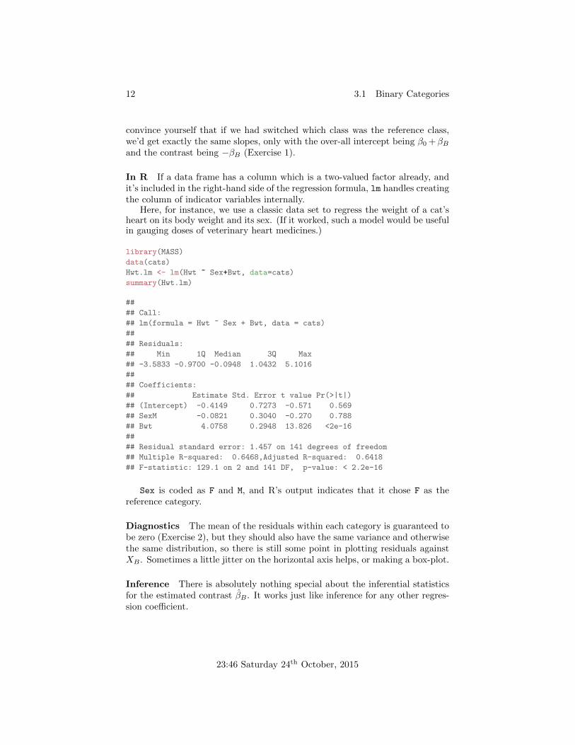
Here, for instance, we use a classic data set to regress the weight of a cat’sheart on its body weight and its sex. (If it worked, such a model would be usefulin gauging doses of veterinary heart medicines.)

library(MASS)

data(cats)

Hwt.lm <- lm(Hwt ~ Sex+Bwt, data=cats)

summary(Hwt.lm)

##

## Call:

## lm(formula = Hwt ~ Sex + Bwt, data = cats)

##

## Residuals:

## Min 1Q Median 3Q Max

## -3.5833 -0.9700 -0.0948 1.0432 5.1016

##

## Coefficients:


## (Intercept) -0.4149 0.7273 -0.571 0.569

## SexM -0.0821 0.3040 -0.270 0.788

## Bwt 4.0758 0.2948 13.826 <2e-16

##

## Residual standard error: 1.457 on 141 degrees of freedom

## Multiple R-squared: 0.6468,Adjusted R-squared: 0.6418

## F-statistic: 129.1 on 2 and 141 DF, p-value: < 2.2e-16

Sex is coded as F and M, and R’s output indicates that it chose F as thereference category.

Diagnostics The mean of the residuals within each category is guaranteed tobe zero (Exercise 2), but they should also have the same variance and otherwisethe same distribution, so there is still some point in plotting residuals againstXB . Sometimes a little jitter on the horizontal axis helps, or making a box-plot.

Inference There is absolutely nothing special about the inferential statisticsfor the estimated contrast βB . It works just like inference for any other regres-sion coefficient.


13 3.1 Binary Categories

Why not just split the data? If we want to give each class its own intercept,why not just split the data and estimate two models, one for each class? Theanswer is that sometimes we’ll do just this, especially if there’s a lot of data foreach class. However, if the regression surfaces for the two categories really areparallel to each other, by splitting the data we’re losing some precision in ourestimate of the common slopes, without gaining anything. In fact, if the twosurfaces are nearly parallel, for moderate sample sizes the small bias that comesfrom pretending the slopes are all equal can be overwhelmed by the reductionin variance.

Why not two columns? It’s natural to wonder why we have to pick outone level as the reference, and estimate a contrast. Why not add two columnsto x, one indicating each class? The problem is that then those two columnswill be linearly dependent (they’ll always add up to one), so the data would becollinear and the model in-estimable.

Why not two slopes? The model we’ve specified has two parallel regressionsurfaces, with the same slopes but different intercepts. We could also have amodel with the same intercept across categories, but different slopes for eachvariable. Geometrically, this would mean that the regression surfaces weren’tparallel, but would meet at the origin (and elsewhere). We’ll see how to makethat work when we deal with interactions in a few lectures. If we wanted differentslopes and intercepts, we might as well just split the data.

Contrasts need contrasts Just as we can’t estimate βi if Var [Xi] = 0, wecan’t estimate any categorical contrasts if all the data points belong to the samecategory.

3.1.1 “Adjusted effect of a category”

As I said, βB is the expected difference in Y between two individuals which havethe same value for all of the variables except the category. This is generally notthe same as the difference in expectations between the two categories:

βB 6= E [Y |XB = 1]− E [Y |XB = 0]

One of the few situations where βB = E [Y |XB = 1]−E [Y |XB = 0] is when thedistribution of all the other variables is the same between the categories. (Saidanother way, the categories are statistically independent of the other predictors.)Another is when there are no other predictors.

Because of this, it’s very natural to want to interpret βB as the differencein the response between the two groups, adjusting for all of the other variables.It’s even common to talk about βB as “the adjusted effect” of the category. Asyou might imagine, such interpretations come up all the time in disputes aboutdiscrimination.

Even leaving aside the emotional charge of such arguments, it is wise to becautious about such interpretations, for several reasons.


14 3.2 Categorical Variables with More than Two Levels

1. The regression is only properly adjusting for all of the other variables ifit’s well-specified. If it’s not, the contrast between the categories will alsopick up some of the average difference in bias (due to getting the modelwrong), which is not relevant.

2. As usual, finding that the contrast coefficient isn’t significant doesn’t nec-essarily mean there is no contrast! It means that the contrast, if thereis one, can’t be reliably distinguished from 0, which could be becauseit’s very small or because we can’t estimate it well. Again as usual, aconfidence interval is called for.

3. It’s not clear that we always do want to adjust for other variables, evenwhen we can measure them. For instance, if economists in Lilliput foundno effect on income between those who broke their eggs at the big endand those at the little end, after adjusting for education and occupa-tional prestige (Swift, 1726), that wouldn’t necessarily settle the questionof whether big-endians were discriminated against. After all, it might bethat they have less access to education and high-paid jobs because theywere big-endians. And this could be true even if Lilliputians were initiallyrandomly assigned between big- and little- end-breaking. The same goesfor finding that there is an “adjusted effect”.

The last point brings us close to topics of causal inference, which we won’tget to until 402. For now, a good rule of thumb is not to adjust for variableswhich might themselves be effects of the variable we’re interested in.

3.2 Categorical Variables with More than Two Levels

Suppose our categorical variable C has more than two levels, say k of them.We can handle it in almost exactly the same way as the binary case. We pickone level — it really doesn’t matter which — as the reference level. We thenintroduce k − 1 columns into the design matrix x, which are indicators for theother categories. If, for instance, k = 3 and the classes are North, South, West,we pick one level, say North, as the reference, and then add a column XSouth

which is 1 for data points in class South and 0 otherwise, and another columnXWest which is 1 for data points in that class and 0 otherwise.

Having added these columns to the design matrix, we regress as usual, andget k−1 contrasts. The over-all β0 is really the intercept for the reference class;the contrasts are added to β0 to get the intercept for each class. Geometrically,we now have k parallel regression surfaces, one for each level of the variable.

Interpretation βC=c is the expected difference between two individuals whoare otherwise identical, except that one is in the reference category and theother is in class c. The expected difference between two otherwise-identicalindividuals in two different categories, say c and d, is therefore the difference intheir contrasts, βC=d − βC=c.


15 3.3 Two, Three, Many Categorical Predictors

Diagnostics and inference Work just the same as in the binary case.

Why not k columns? Because, just like in the binary case, that would makeall those columns for that variable sum to 1, causing problems with collinearity.

Contrasts need contrast If we know there are k categories, but some ofthem don’t appear in our data, we can’t estimate their contrasts.

Category-specific slopes and splitting the data The same remarks applyas under binary predictor variables.

3.3 Two, Three, Many Categorical Predictors

Nothing in what we did above requires that there be only one categorical pre-dictor; the other variables in the model could be indicator variables for othercategorical predictors. Nor do all the categorical predictors have to have thesame number of categories. The only wrinkle with having multiple categoriesis that β0, the over-all intercept, is now the intercept for individuals where allcategorical variables are in their respective reference levels. Each combinationof categories gets its own regression surface, still parallel to each other.

With multiple categories, it is natural to want to look at interactions — tolet their be an intercept for left-handed little-endian plumber, rather than justadding up contrasts for being left-handed and being a little-endian and being aplumber. We’ll look at that when we deal with interactions.

3.4 Analysis of Variance: Only Categorical Predictors

A model in which there are only categorical predictors is, for historical reasons,often called an analysis of variance model. Estimating such a model presentsabsolutely no special features beyond what we have already covered, but it’sworth a paragraph or two on the interpretation and the origins of such models.

Suppose, for simplicity, that there are two categorical predictors, B and C,and the reference level for each is written ∅. The conditional expectation of Ywill be pinned down by giving a level for each, say b and c, respectively. Then

E [Y |B = b, C = c] = β0 + βbδb∅ + βcδc∅

That is, we add the appropriate contrast for each categorical variable, and noth-ing else. (This presumes no interactions, a limitation which we’ll lift next week.)Conversely, if we knew E [Y |B = b, C = c] for every category, we could work outthe contrasts without having to ever (explicitly) compute (xTx)−1xTy, whichwas a very real consideration before computation became so cheap5. Obviously,however, it is not much of an issue now.

5To see how, notice that β0 can be estimated by the sample mean of all cases whereB = ∅, C = ∅. Then to get, say, βb, we average the difference in means between cases whereB = b, C = c and B = ∅, C = c for each level c of the other variable. (This averaging ofdifferences eliminates the contribution from βc.)


16 3.5 Ordinal Variables

As for the name, it arises from the basic probability fact sometimes calledthe “law of total variance”:

Var [Y ] = Var [E [Y |X]] + E [Var [Y |X]]

If X is our complete set of categorical variables, each of which defines a group,this says “The total variance of the response is the variance in average responsesacross groups, plus the average variance within a group”. Thus, after estimatingthe contrasts, we have decomposed or analyzed the variance in Y into between-group and across-group variance. This was extremely useful in the early daysof agricultural and industrial experimentation, but has frankly become a bit ofa fossil, if not a fetish.

An “analysis of covariance” model is just a regression with both qualitativeand quantitative predictors.

3.5 Ordinal Variables

An ordinal variable, as I said, is one where the qualitatively-distinct levels canbe put in a sensible order, but there’s no implication that the distance fromone level to the next is constant. At our present level of sophistication, we havebasically two ways to handle them:

1. Ignoring the ordering and treat them like nominal categorical variables.

2. Ignoring the fact that they’re only ordinal and not metric, assign themnumerical codes (say 1, 2, 3, . . . ) and treat them like ordinary numericalvariables.

The first procedure is unbiased, but can end up dealing with a lot of distinctcoefficients. It also has the drawback that if the relationship between Y and thecategorical variable is monotone, that may not be respected by the coefficientswe estimate. The second procedure is very easy, but usually without any sub-stantive or logical basis. It implies that each step up in the ordinal variable willpredict exactly the same difference in Y , and why should that be the case? If,after treating an ordinal variable like a nominal one, we get contrasts which areall (approximately) equally spaced, we might then try the second approach.

Other procedures for ordinal variables which are, perhaps, more conceptuallysatisfying need much more math than we’re presuming here; see the furtherreading.

3.6 Detailed R Example

The data set for the first data analysis project included a categorical variable,State, which we did not use. Let’s try adding it to the model.

First, let’s do some basic counting and examination:


17 3.6 Detailed R Example

# How many levels does State have?

nlevels(mobility$State)

## [1] 51

# What are they?

levels(mobility$State)

## [1] "AK" "AL" "AR" "AZ" "CA" "CO" "CT" "DC" "DE" "FL" "GA" "HI" "IA" "ID"

## [15] "IL" "IN" "KS" "KY" "LA" "MA" "MD" "ME" "MI" "MN" "MO" "MS" "MT" "NC"

## [29] "ND" "NE" "NH" "NJ" "NM" "NV" "NY" "OH" "OK" "OR" "PA" "RI" "SC" "SD"

## [43] "TN" "TX" "UT" "VA" "VT" "WA" "WI" "WV" "WY"

There are 51 levels for State, as there should be, corresponding to the 50states and the District of Columbia. We see that these are given by the two-letter postal codes, in alphabetical order.

Running a model with State and Commute as the predictors, we thereforeexpect to get 52 coefficients (1 intercept, 1 slope, and 51-1 = 50 contrasts). Rwill calculate contrasts from the first level, which here is AK, or Alaska.

mob.state <- lm(Mobility ~ Commute + State, data=mobility)

signif(coefficients(mob.state),3)

## (Intercept) Commute StateAL StateAR StateAZ StateCA

## 0.018400 0.126000 -0.005600 0.001840 0.007290 0.031500

## StateCO StateCT StateDC StateDE StateFL StateGA

## 0.044100 0.021500 0.071300 0.007460 0.004160 -0.022000

## StateHI StateIA StateID StateIL StateIN StateKS

## 0.029100 0.052200 0.029700 0.013200 0.010000 0.042400

## StateKY StateLA StateMA StateMD StateME StateMI

## 0.011900 0.021100 0.001230 0.018700 0.004710 0.005230

## StateMN StateMO StateMS StateMT StateNC StateND

## 0.055300 0.011900 -0.018700 0.045200 -0.011400 0.146000

## StateNE StateNH StateNJ StateNM StateNV StateNY

## 0.060400 0.032200 0.062700 0.006670 0.045400 0.022300

## StateOH StateOK StateOR StatePA StateRI StateSC

## -0.000559 0.036000 0.013800 0.035000 0.022400 -0.019300

## StateSD StateTN StateTX StateUT StateVA StateVT

## 0.042300 0.000761 0.032200 0.060500 0.014100 0.017300

## StateWA StateWI StateWV StateWY

## 0.025800 0.031700 0.057800 0.061200

In the interest of space, I won’t run summary on this, but you can. You willfind that quite a few of the contrasts are statistically significant. We’d expectabout 50 × 0.05 = 2.5 to be significant at the 5% level, even if all the truecontrasts were zero, but many more them are than this baseline. As usual, ofcourse, it doesn’t mean the model is right; it just means that if we were goingto put in an intercept, a slope for Commute, and a contrast for every other state,we should really put in contrasts for those states as well.



# Set up a function to make maps

# "Terrain" color levels set based on quantiles of the variable being plotted

# Inputs: vector to be mapped over the data frame; number of levels to

# use for colors; other plotting arguments

# Outputs: invisibly, list giving cut-points and the level each observation

# was assigned

mapper <- function(z, levels, ...) {# Which quantiles do we need?

probs <- seq(from=0, to=1, length.out=(levels+1))

# What are those quantiles?

z.quantiles <- quantile(z, probs)

# Assign each observation to its quantile

z.categories <- cut(z, z.quantiles, include.lowest=TRUE)

# Make up a color scale

shades <- terrain.colors(levels)

plot(x=mobility$Longitude, y=mobility$Latitude,

col=shades[z.categories], ...)

invisible(list(quantiles=z.quantiles, categories=z.categories))

}

Figure 2: Function for making maps, from the model DAP 1.

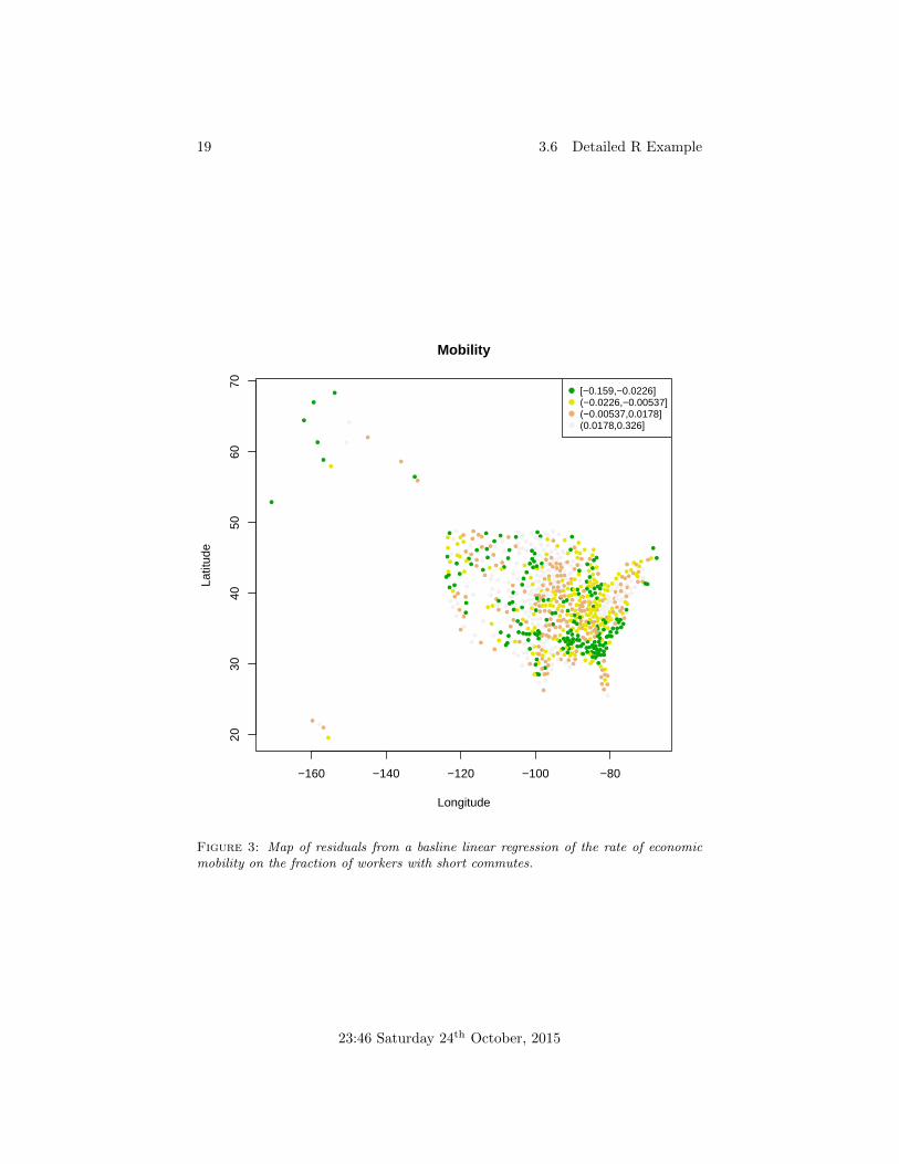
One issue with the simple linear regression from the DAP was that its resid-uals were very strongly correlated spatially. We might hope that adding allthese state-by-state contrasts has gotten rid of some of that correlation.

When we have a large number of categories, it’s often tempting to try com-pressing them to a smaller number, by grouping together some of the levels.If we do this right, we reduce the variance in our estimates of the coefficients,while introducing little (if any) bias.

To illustrate this, let’s try boiling down the 51 states (and DC) into two cat-egories: the South versus the rest of the country. The South has long been quitedistinct from the rest of the country culturally, politically and economically, inways which are, plausibly, very relevant to economic mobility. More relevantly,when we looked at the residuals in the DAP, there was a big cluster of negativeresiduals in the southeastern part of the map. To make this concrete, I’ll definethe South as consisting of those states which joined the Confederacy during theCivil War (Alabama, Arkansas, Florida, Georgia, Louisiana, Mississippi, NorthCarolina, South Carolina, Tennessee, Texas and Virginia).

Let’s start by adding the relevant column to the data frame:

# The states of the Confederacy

Confederacy <- c("AR", "AL", "FL", "GA", "LA", "MS", "NC", "SC", "TN", "TX", "VA")

mobility$Dixie <- mobility$State %in% Confederacy

The new Dixie column of mobility will contain the values TRUE, for eachcommunity located in one of those states, and FALSE, for the rest. R will insuch circumstances treat FALSE as the reference category.



●●●

● ●●●●

●

●●

●

●●●

●●●

●●●

●●

●●●

● ●

●

●

●● ●

●

●

●

●●

●●●

●●●●

●

●●

●

●

●●

●●

●

●●

●

●●●

●●

●

●●●

●●●

●

●

●

●●

●

●

●●

●●

●●

●●●

●●

●●

●

●●

●

●

●

●

●

●●

●

●

●

●

●●

●

●●

●●

●●

● ●

●

●●

●●

●●●●

●●

●●

●●

●

●

●●●

●●

●●●

●●

●●●●

●

●

●●●

●

●●

●

●●

●●

●●

●

●

●

●

●

●●

●

●

●●

● ●●●

●

●

●●

●●

●

●●

●●

●

●●●●

●●

●●

●●

●●●●●

●●

●

●

●

●

●

●

●●●

●

●

●●

●●

●

●●●

●

● ●●

●●

●

●

●●●

●

●●

●

●●

●

●

●●●

●

●

●●

●●●

●

● ●

●●

●●●●

●●

●

●

●

●

●●

●●

●

● ●

●

●

●●

●

●●●

●

●●

●

●

●

●

●

●

●●●

●●● ●

●●

●

●

●●

● ●

●

●●

●●

●

●●

●●●●

●

●●

●

●●

●●

● ●

●●

●

●●

●

●●

● ●

●●

●●

●●

●

●

●●●

●

●●●

●

● ●

●●

●●

●

●●

●

●●●

●●●

●

●

●

●●

●●●

●

● ●●

●

●

●

● ●

●●

●●

●

●

●●●

●●

●

●●●

●●

●

●●

●

●

●

●

●

●●

●

●

●●● ●

●

●●

●●

● ●

●

●

●●

●

●

●●

●

●

●

●

●●

●

●●

●●

● ●●

●

●

●

●●

●

●●

●

●●

●

●●●

●●

●●

●●

●

●

●

●

●●

●●●●

●●

●

●●

●●

●●

●●

●

●

●

●●

●

●●

●

●

● ●

●

●

●

●●

●

●●●

●● ●

●

●●

●

●●●

●

●

●

●●

●●

●

●●

●●

●●

●

●

●●

●

●

●●

●●

●

●

●●

●●

●

●

●●

●

●

●

●

●

●

●●

●● ●

●

●●

●

●●●

●

●

●●

●●

●

●● ● ●●

●● ●

●●

●

●●●

●

●●●

●

● ●●

●

●

●

●

●

●

●

●●

●

●

●

●

●●

● ●

●●

●

●

●●●

●

●●

●●

●●

●

●

●

●

●

●●

●

●●●

●

●

●

●●

●

●

●●

●

●

●

●

●

●

●

●●●

●

●●

● ●

●

●

●

●

●

●

●●

●●

●

●●

●●

●●

●

●

●

●

●

●

●

●

●

●●

●

●

●

●

●

● ●

●

●

●●

●● ●

●

●

● ●

●

●

●

●

●●

●

●●

●●

●●

−160 −140 −120 −100 −80

2030

4050

6070

Mobility

Longitude

Latit

ude

●

●

●

●

[−0.159,−0.0226](−0.0226,−0.00537](−0.00537,0.0178](0.0178,0.326]

Figure 3: Map of residuals from a basline linear regression of the rate of economicmobility on the fraction of workers with short commutes.



●●●

● ●●●●

●

●●

●

●●●

●●●

●●●

●●

●●●

● ●

●

●

●● ●

●

●

●

●●

●●●

●●●●

●

●●

●

●

●●

●●

●

●●

●

●●●

●●

●

●●●

●●●

●

●

●

●●

●

●

●●

●●

●●

●●●

●●

●●

●

●●

●

●

●

●

●

●●

●

●

●

●

●●

●

●●

●●

●●

● ●

●

●●

●●

●●●●

●●

●●

●●

●

●

●●●

●●

●●●

●●

●●●●

●

●

●●●

●

●●

●

●●

●●

●●

●

●

●

●

●

●●

●

●

●●

● ●●●

●

●

●●

●●

●

●●

●●

●

●●●●

●●

●●

●●

●●●●●

●●

●

●

●

●

●

●

●●●

●

●

●●

●●

●

●●●

●

● ●●

●●

●

●

●●●

●

●●

●

●●

●

●

●●●

●

●

●●

●●●

●

● ●

●●

●●●●

●●

●

●

●

●

●●

●●

●

● ●

●

●

●●

●

●●●

●

●●

●

●

●

●

●

●

●●●

●●● ●

●●

●

●

●●

● ●

●

●●

●●

●

●●

●●●●

●

●●

●

●●

●●

● ●

●●

●

●●

●

●●

● ●

●●

●●

●●

●

●

●●●

●

●●●

●

● ●

●●

●●

●

●●

●

●●●

●●●

●

●

●

●●

●●●

●

● ●●

●

●

●

● ●

●●

●●

●

●

●●●

●●

●

●●●

●●

●

●●

●

●

●

●

●

●●

●

●

●●● ●

●

●●

●●

● ●

●

●

●●

●

●

●●

●

●

●

●

●●

●

●●

●●

● ●●

●

●

●

●●

●

●●

●

●●

●

●●●

●●

●●

●●

●

●

●

●

●●

●●●●

●●

●

●●

●●

●●

●●

●

●

●

●●

●

●●

●

●

● ●

●

●

●

●●

●

●●●

●● ●

●

●●

●

●●●

●

●

●

●●

●●

●

●●

●●

●●

●

●

●●

●

●

●●

●●

●

●

●●

●●

●

●

●●

●

●

●

●

●

●

●●

●● ●

●

●●

●

●●●

●

●

●●

●●

●

●● ● ●●

●● ●

●●

●

●●●

●

●●●

●

● ●●

●

●

●

●

●

●

●

●●

●

●

●

●

●●

● ●

●●

●

●

●●●

●

●●

●●

●●

●

●

●

●

●

●●

●

●●●

●

●

●

●●

●

●

●●

●

●

●

●

●

●

●

●●●

●

●●

● ●

●

●

●

●

●

●

●●

●●

●

●●

●●

●●

●

●

●

●

●

●

●

●

●

●●

●

●

●

●

●

● ●

●

●

●●

●● ●

●

●

● ●

●

●

●

●

●●

●

●●

●●

●●

−160 −140 −120 −100 −80

2030

4050

6070

Mobility

Longitude

Latit

ude

●

●

●

●

[−0.154,−0.0166](−0.0166,−0.00246](−0.00246,0.0115](0.0115,0.223]

residuals.state.map <- mapper(residuals(mob.state), levels=4, pch=19,

cex=0.5, xlab="Longitude", ylab="Latitude",

main="Mobility")

legend("topright", legend=levels(residuals.state.map$categories), pch=19,

col=terrain.colors(4), cex=0.8)

Figure 4: Map of the residuals for the model with state-level contrasts. (See Figure2 for the mapper function.)



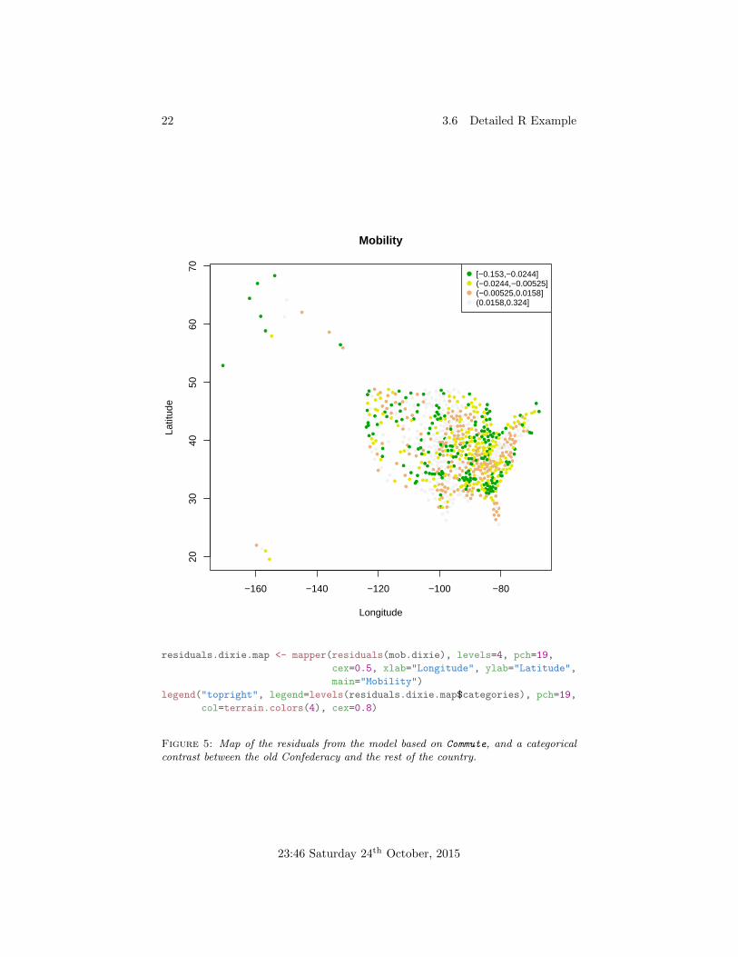
mob.dixie <- lm(Mobility ~ Commute + Dixie, data=mobility)

signif(coefficients(summary(mob.dixie)),3)


## (Intercept) 0.0190 0.00607 3.13 1.84e-03

## Commute 0.1950 0.01180 16.50 2.94e-52

## DixieTRUE -0.0217 0.00354 -6.14 1.37e-09

The contrast for the old Confederacy versus the rest of the country is neg-ative, meaning those states have lower levels of economic mobility, and highlystatistically significant. Of course, the model could still be wrong. The resid-uals, while better than a model with no geographic contrasts, don’t look asrandom as in the one with contrasts for each state.



●●●

● ●●●●

●

●●

●

●●●

●●●

●●●

●●

●●●

● ●

●

●

●● ●

●

●

●

●●

●●●

●●●●

●

●●

●

●

●●

●●

●

●●

●

●●●

●●

●

●●●

●●●

●

●

●

●●

●

●

●●

●●

●●

●●●

●●

●●

●

●●

●

●

●

●

●

●●

●

●

●

●

●●

●

●●

●●

●●

● ●

●

●●

●●

●●●●

●●

●●

●●

●

●

●●●

●●

●●●

●●

●●●●

●

●

●●●

●

●●

●

●●

●●

●●

●

●

●

●

●

●●

●

●

●●

● ●●●

●

●

●●

●●

●

●●

●●

●

●●●●

●●

●●

●●

●●●●●

●●

●

●

●

●

●

●

●●●

●

●

●●

●●

●

●●●

●

● ●●

●●

●

●

●●●

●

●●

●

●●

●

●

●●●

●

●

●●

●●●

●

● ●

●●

●●●●

●●

●

●

●

●

●●

●●

●

● ●

●

●

●●

●

●●●

●

●●

●

●

●

●

●

●

●●●

●●● ●

●●

●

●

●●

● ●

●

●●

●●

●

●●

●●●●

●

●●

●

●●

●●

● ●

●●

●

●●

●

●●

● ●

●●

●●

●●

●

●

●●●

●

●●●

●

● ●

●●

●●

●

●●

●

●●●

●●●

●

●

●

●●

●●●

●

● ●●

●

●

●

● ●

●●

●●

●

●

●●●

●●

●

●●●

●●

●

●●

●

●

●

●

●

●●

●

●

●●● ●

●

●●

●●

● ●

●

●

●●

●

●

●●

●

●

●

●

●●

●

●●

●●

● ●●

●

●

●

●●

●

●●

●

●●

●

●●●

●●

●●

●●

●

●

●

●

●●

●●●●

●●

●

●●

●●

●●

●●

●

●

●

●●

●

●●

●

●

● ●

●

●

●

●●

●

●●●

●● ●

●

●●

●

●●●

●

●

●

●●

●●

●

●●

●●

●●

●

●

●●

●

●

●●

●●

●

●

●●

●●

●

●

●●

●

●

●

●

●

●

●●

●● ●

●

●●

●

●●●

●

●

●●

●●

●

●● ● ●●

●● ●

●●

●

●●●

●

●●●

●

● ●●

●

●

●

●

●

●

●

●●

●

●

●

●

●●

● ●

●●

●

●

●●●

●

●●

●●

●●

●

●

●

●

●

●●

●

●●●

●

●

●

●●

●

●

●●

●

●

●

●

●

●

●

●●●

●

●●

● ●

●

●

●

●

●

●

●●

●●

●

●●

●●

●●

●

●

●

●

●

●

●

●

●

●●

●

●

●

●

●

● ●

●

●

●●

●● ●

●

●

● ●

●

●

●

●

●●

●

●●

●●

●●

−160 −140 −120 −100 −80

2030

4050

6070

Mobility

Longitude

Latit

ude

●

●

●

●

[−0.153,−0.0244](−0.0244,−0.00525](−0.00525,0.0158](0.0158,0.324]

residuals.dixie.map <- mapper(residuals(mob.dixie), levels=4, pch=19,

cex=0.5, xlab="Longitude", ylab="Latitude",

main="Mobility")

legend("topright", legend=levels(residuals.dixie.map$categories), pch=19,

col=terrain.colors(4), cex=0.8)

Figure 5: Map of the residuals from the model based on Commute, and a categoricalcontrast between the old Confederacy and the rest of the country.


23

4 Further Reading

Polynomial regression and categorical predictors are both ancient topics; I don’tknow who first introduced either.

The above discussion has assumed that when we use a polynomial, we usethe same polynomial for all values of Xi. An alternative is to use different, low-order polynomials in different regions. If these piecewise polynomial functionsare required to be continuous, they are called splines, and regression withsplines will occupy us for much of 402, because it gives us ways to tackle lotsof the issues with polynomials, like over-fitting (Shalizi, forthcoming, chs. 8 and9). Personally, I have found splines to almost always be a better tool thanpolynomial regression, but they do demand a bit more math.

The matter of “adjusted effects” and causal inference will occupy us forabout the last quarter of 36-402.

Tutz (2012) is a thorough and modern survey of regression with categoricalresponse variables. We will go over this in some detail in 402, but his bookcovers many topics we won’t have time for.

Winship and Mare (1984) proposes some interesting techniques for dealingwith ordinal variables, under the (strong) assumption that they arise from tak-ing continuous variables and breaking them into discrete categories. This seemsto require rather strong assumptions about the measurement process. Anotherdirection we could go would be to estimate a separate contrast for each levelof an ordinal variable (except the lowest), but require these to be either all in-creasing or all decreasing, so the response to the ordinal variable was monotone.This would mean solving a constrained least squares (or maximum likelihood)problem to get the estimates, not an unconstrained on. Worse, the constraintswould be a somewhat awkward set of inequalities. Still, it’s do-able in principle,though I don’t know of a straightforward R implementation.

Analysis of variance models were introduced by R. A. Fisher, probably thegreatest statistician who ever lived, in connection with problems in geneticsand in designing and interpreting experiments. They have given rise to a hugeliterature and an elaborate system of notation and terminology, much of whichboils down to short-cuts for computing regression estimates when the designmatrix x has very special structure. As I said, there were many decades whensuch short-cuts were vital, but I am frankly skeptical how much value thesetechniques retain in the present day. In the interest of balance, see Gelman(2005) for a contrary view.

I mentioned that one reason to use polynomials is that any well-behavedfunction can be approximated arbitrarily closely by polynomials of sufficientlyhigh degree. Obviously “well-behaved” needs a proper definition, as (perhapsless obviously) does “approximated arbitrarily closely”. What I had in mind wasthe Stone-Weierstrass theorem, which states that you can pick any continuousfunction f , interval [a, b], and tolerance ε > 0 you like, and I can find some


24

polynomial which is within ε of f everywhere on the interval,

maxa≤x≤b

∣∣∣∣∣∣f(x)−d∑

j=1

γjxj

∣∣∣∣∣∣ ≤ εprovided there is no limit on the order d or the magnitude of the coefficients γj .This is a standard result of real analysis, which will be found in almost textbookon that subject, or on functional analysis or approximation theory. There areparallel results for other function bases.

5 Exercises

To think through or practice on, not to hand in.

1. Consider regressing Y on a binary categorical variable B, plus some otherpredictors. Suppose we switch which level is the reference category andwhich one is contrasted with it. Show that this produces the followingchanges to the parameters, and leaves all the others unchanged:

β0 → β0 + βB (1)

βB → −βB (2)

Hint: Show that the change to the indicator variable is XB → 1−XB .

2. Consider again regressing Y on a binary variable B, plus some other pre-dictors, and estimating all coefficients by least squares. Show that theaverage of all residuals where XB = 1 must be exactly 0, as must the av-erage of all residuals where XB = 0. Hint: Use the estimating equationsto show

∑i ei = 0,

∑i eixBi = 0, and algebra to show

∑i ei(1− xBi) = 0.

References

Gelman, Andrew (2005). “Analysis of Variance — Why It Is More Importantthan Ever.” Annals of Statistics, 33: 1–53. URL http://projecteuclid.

org/euclid.aos/1112967698. doi:10.1214/009053604000001048.

Shalizi, Cosma Rohilla (forthcoming). Advanced Data Analysis from an Elemn-tary Point of View . Cambridge, England: Cambridge University Press. URLhttp://www.stat.cmu/~cshalizi/ADAfaEPoV.

Swift, Jonathan (1726). Gulliver’s Travels. London: Benjamin Motte. URLhttp://www.gutenberg.org/ebooks/829. Originally published as Travelsinto Several Remote Nations of the World. In Four Parts. By Lemuel Gulliver,First a Surgeon, and then a Captain of several Ships.

Tutz, Gerhard (2012). Regression for Categorical Data. Cambridge, England:Cambridge University Press.


http://projecteuclid.org/euclid.aos/1112967698

http://projecteuclid.org/euclid.aos/1112967698

http://dx.doi.org/10.1214/009053604000001048

http://www.stat.cmu/~cshalizi/ADAfaEPoV

http://www.gutenberg.org/ebooks/829

25 REFERENCES

Winship, Christopher and Robert D. Mare (1984). “Regression Models withOrdinal Variables.” American Sociological Review , 49: 512–525. URL http:

//scholar.harvard.edu/files/cwinship/files/asr_1984.pdf.


http://scholar.harvard.edu/files/cwinship/files/asr_1984.pdf

http://scholar.harvard.edu/files/cwinship/files/asr_1984.pdf

lecture 16: polynomial and categorical regressioncshalizi/mreg/15/lectures/lecture-16.pdflecture 16:...

Documents