lecture 19 wind and turbulence part 4 surface boundary ... · espm 129 biometeorology, wind and...

ESPM 129 Biometeorology, Wind and Turbulence, part 4

1

Lecture 19, Wind and Turbulence, Part 4, Surface Boundary Layer: Theory and Principles, Cont Instructor: Dennis Baldocchi Professor of Biometeorology Ecosystem Science Division Department of Environmental Science, Policy and Management 345 Hilgard Hall University of California, Berkeley Berkeley, CA 94720 October 17, 2014 Topics to Be Covered A. Variation in Time 1. Statistical Representation of Turbulence

a. Time series of w,u,T,Q,C b. Reynold’s averaging c. Variances (turbulence intensities) d. Covariances e. probability distributions

2. Parameterizations and Observations a. non-dimensional functions for standard deviations in w and u

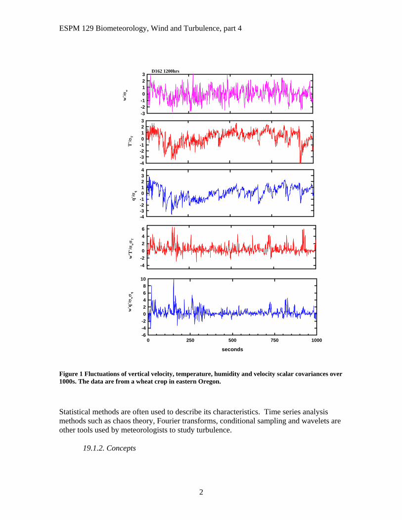
B. Spectrum of turbulence a. Power Spectra/ Co-spectra b. inertial subrange c. Engineering formulae for spectra L19.1 Variation in Time L19.1.1 Time series of Turbulence Quantities, w ,u, T, Q, C Time courses of turbulence velocity vectors and scalars contain both fine and coarse grain fluctuations.


2

Figure 1 Fluctuations of vertical velocity, temperature, humidity and velocity scalar covariances over 1000s. The data are from a wheat crop in eastern Oregon.

Statistical methods are often used to describe its characteristics. Time series analysis methods such as chaos theory, Fourier transforms, conditional sampling and wavelets are other tools used by meteorologists to study turbulence.

19.1.2. Concepts

D162 1200hrs

w'q

'/ w q

w'T

'/ w T

seconds

0 250 500 750 1000-6

-4

-2

0

2

4

6

8

10

-4

-2

0

2

4

6

q'/

q

-4-3-2-101234

-4-3-2-10123

T'/ T

-3-2-10123

w'/

w


3

Reynolds’ averaging is used to provide a statistical representation of turbulence. In a turbulent fluid its components can be defined in any instant of time as being a function of

the mean state of the fluid (u,v,w,T, c) plus its fluctuation from the mean: x x x ' This assumption yielded several interesting properties: 1) the mean product of two components is a function of the product of the individual means plus a covariance:

xy x y x y ' ' 2) the average of any fluctuating component is zero:

x' 0 3) the average of the sum of components is additive:

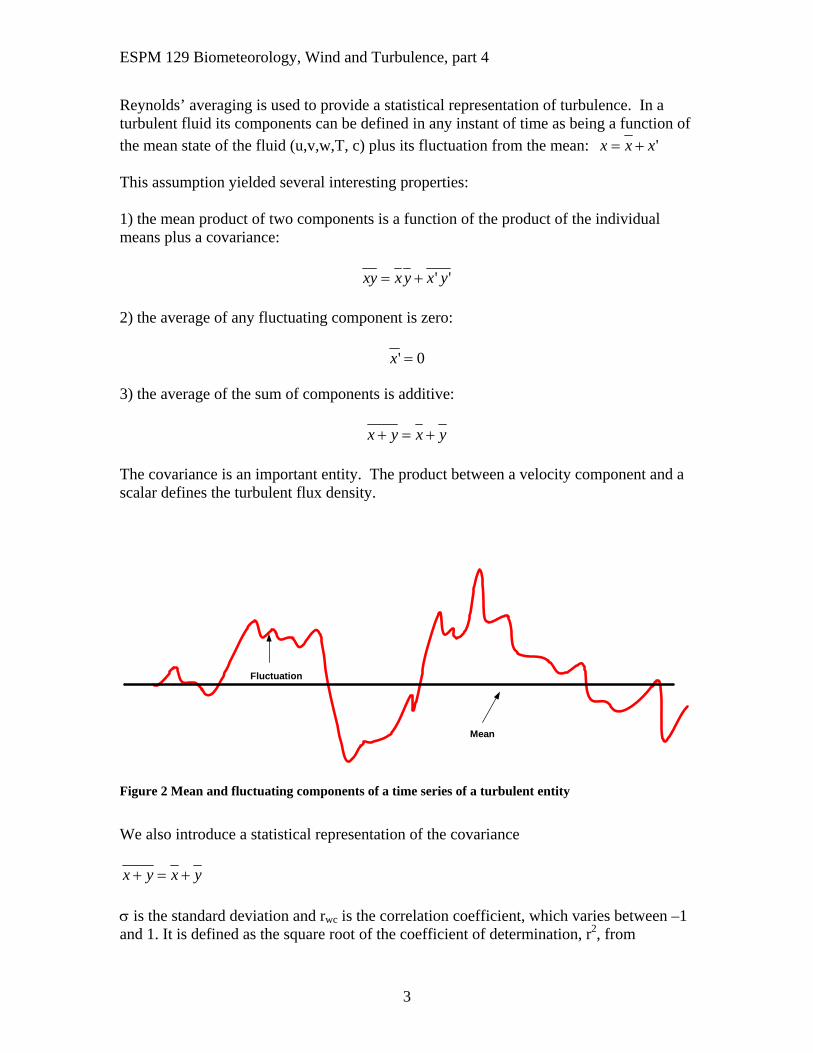
x y x y The covariance is an important entity. The product between a velocity component and a scalar defines the turbulent flux density.

Figure 2 Mean and fluctuating components of a time series of a turbulent entity

We also introduce a statistical representation of the covariance

x y x y is the standard deviation and rwc is the correlation coefficient, which varies between –1 and 1. It is defined as the square root of the coefficient of determination, r2, from

Mean

Fluctuation


4

regression theory. For wu the correlation coefficient is about –0.35 for |z/L| +/- 1. For wT , r is about –0.4 for stable conditions and 0.5 for unstable conditions. Later in this lecture we’ll derive the correlation coefficient. The variance is defined as:

( )( )

xx x

n

in2

2

1

If turbulence is homogeneous and stationary, time and space averages should be identical. This is the ergodic condition 21.1.3 Wind and Turbulence statistics The wind movement is comprised of three velocity components, which correspond to the three Cartesian directions, x, y and z. u is the horizontal streamwise velocity, v is the horizontal lateral velocity and w is the vertical velocity. Instantaneous velocity measurements consist of the mean component and the fluctuation from the mean.

u u u '

v v v '

w w w ' With regard to vertical velocity, the mean vertical velocity is typically zero over flat terrain. The mean component of turbulence

fT

fdtt

t

T

T

z1

0 2

0 2

Wind speed is defined as:

U u v w ( )2 2 2 12

We have to be careful when evaluating vector and scalar products. Wind speed is a scalar. It is not equal to its vector sums because of nuanances associated with products of fluctuating components


5

U u v w u v w ( ) ( )2 2 2 2 2 212

12

U u v w

u u u u v v v v w w w w

u v w u u v v w w

( )

[( ' )( ' ) ( ' )( ' ) ( ' )( ' )]

( ' ' ' ' ' ')

2 2 2

2 2 2

12

12

12

In a similar manner based:

( ' ' ' ' ( ' ' ' ' )w u w v w u w v2 2 2

Sweeps and ejections are very non-Gaussian, and they retain sign information, being vector quantities. Hence, momentum transfer is a vector quantity. It has direction and magnitude.

The standard deviation is the square root of the variance and turbulence intensity is the normalized standard deviation, by wind speed or friction velocity.

iu

uu

Skewness defines the assymetric of a probability distribution

Sku

u '3

3

Skewness is zero for a normal distribution, it is greater than one when the mode is less than the mean and the tail is skewed towards larger values a Gaussian distribution. Skewness is less than zero when the mode is greater than the mean, and extreme values are skewed towards values smaller than the smaller tail of the Gaussian distribution. Kurtosis defines the flatness or peakedness of a probability distribution

Kru

u '4

4

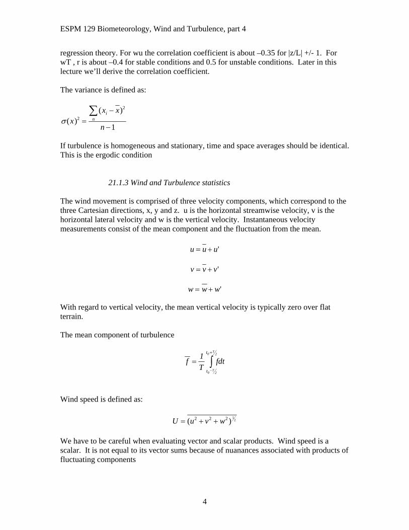
Kurtosis equals 3 for a normal or Gaussian distribution, it is less than 3 for a flat distribution and greater than 3 for a peaked distribution. Probability distributions of a turbulence are shown below. The behavior of turbulence is markedly non-Gaussian. In general Sku is greater than zero and Skw is less than zero. Sku


6

is positive because intermittent gusts penetrate deep into the canopy, having velocities greater than the local mean. Skw is negative because turbulence with fluctuations greater than the mean are carried downward with the large gusts, while there is no equivalent source for upward motion because the ground suppresses turbulent motions.

Figure 3 probablity distribution of vertical wind velocity

jackpineD2431200

w (m s-1)

-3 -2 -1 0 1 2 3

pd

f

0.00

0.01

0.02

0.03

0.04

0.05


7

Figure 4 probability distribution for horizontal wind speed over a jack pine forest.

We also observe that the probability distributions of temperature are skewed.

Interestingly, if we examine the probability distribution of sequential fluctuations, we find those are normally distributed (Liukang Xu, personal communication).

wind speed

0 1 2 3 4 5 6

Freq

uenc

y

0.000

0.001

0.002

0.003

0.004

0.005

0.006

0

0.01

0.02

0.03

0.04

0.05

0.06

16 17 18 19 20 21

PD

F

Ts


8

21.1.4 Averaging Problem in turbulence. How long is enough? We desire to attain an ensemble average, who's average attains a stable value as the time interval increases.

Tf

f 2

12

2 2

'

is the turbulence time scale and is the error. For neutral conditions and for the variance of w or temperature, the mean sampling time should be on the order of:

Tz

u

42

for w’T’ and w’u’

Tz

u

202

For unstable For w’2 and T’2

Tz

u

42

For w’u’

0

0.02

0.04

0.06

0.08

0.1

0.12

0.14

0.16

-1.5 -1 -0.5 0 0.5 1 1.5

PD

F

Delta_Ts


9

Tz

u

1002

and for w’T’

Tz

u

122

Integration time (minutes) for variance of scalars and covariances, after Sreenivasan ete al. 1978. variable .1 U2 12.1 W2 3.4 T2 18 Q2 10.8 W’u’2 20.4 Wq2 10.3 W’T’2 15.8 19.2 Parameterizing Turbulence Statistics Monin-Obuhkov scaling theory gives us a framework to examine how turbulence statistics scale with friction velocity and stability. But it does not provide us with any information on the magnitude. Over the years numerous studies have been conducted that assess mean, normalized turbulence statistics under different thermal stratification regimes. Stull (Stull, 1988) has surveyed many of these studies. Values of important parameters are listed below. Stable Boundary Layer

w

u*

. 158

*

2

U

u*

. 2 91

Convective or Unstable Conditions


10

w

u

z

L*

/. ( ) 19 1 3

*

/. ( ) 0 95 1 3z

L

Alternatively, Panofsky parameterize standard deviations in w for unstable thermal stratification as: w

u

z

L*

/. ( | | ) 125 1 3 1 3

and he assumes that w

u*

under stable conditions is the same as the near neutral value of

1.25, since it is so difficult to measure these quantities under stable conditions. Under near neutral conditions we can compute these ratios as:

w

u*

. 13

*

2

u

u*

. 2 49

v

u*

. 173

U

u*

. 2 91


11

z/L

-4 -3 -2 -1 0 1 2 3

w/u

*

1.0

1.2

1.4

1.6

1.8

2.0

2.2

2.4

2.6

2.8

Figure 5 standard deviation of w scaled with friction velocity, after parameterization of Panofsky.

During unstable conditions, horizontal wind velocity fluctuations scale with the height of the planetary boundary layer, zi.

u i

u

z

L*

/( . ) 12 05 1 3


12

zi/L

-500 -400 -300 -200 -100 0

u/u

*

2

3

4

5

6

7

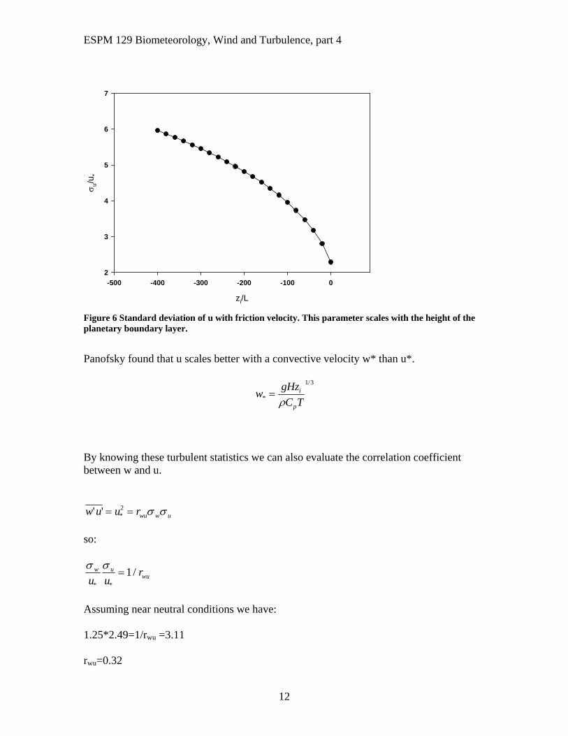
Figure 6 Standard deviation of u with friction velocity. This parameter scales with the height of the planetary boundary layer.

Panofsky found that u scales better with a convective velocity w* than u*.

wgHz

C Ti

p*

/

1 3

By knowing these turbulent statistics we can also evaluate the correlation coefficient between w and u.

w u u rwu w u' ' * 2 so: w u

wuu ur

* *

/1

Assuming near neutral conditions we have: 1.25*2.49=1/rwu =3.11 rwu=0.32


13

Most numerical schemes apply the fast Fourier technique to time series that contain a number of samples that is a power of two. In principle, Taylor’s frozen eddy hypothesis is invoked when computing spectra. This comment is made because spectra are derived from the Fourier transform of the lag correlation function:

R x r u x u x r( , ) ' ( ) ' ( ) One assumes temporal measurements of wind can be used to deduce spatial properties (x=u t). Eddy shapes evolve over a longer time scale than it takes for the eddies to pass a senor. For an illustration, compare the lifetime of the eddies () with the time to advect past an instrument mast (T=/U). Want >> T.

T

Uu

It tends to hold if the turbulence intensity is less than about 0.5. Atmospheric spectra consist of three subranges, the energy containing range, the inertial subrange and the dissipation range. The turbulence in the energy containing range is produced by shear and buoyancy. In the inertial subrange, energy is neither produced or destroyed. Instead energy cascades from larger to smaller scales. The spectrum in the inertial subrange:

Su ( ) / / 2 3 5 3 The coefficient is the Kolmogorov constant. This equation shows that the slope of the spectrum in the inertial subrange has a slope of –5/3 (or –2/3 when normalized by n). The spectra in this range also conforms to local isotropy. Correlations between velocity components are nil and there is no net transfer of turbulence in this subrange. In contrast, the co-spectrum possesses a –7/3 slope in the inertial subrange (or –4/3 when normalized by n). The dissipation, or Kolmogorov, length scale is defined as a ratio between the kinematic viscosity and the rate of tke dissipation, :

( ) /3

1 4


14

The length scale is on the order of 0.001 m Rarely is wavenumber measured (except with aircraft, flying through ‘frozen’ turbulence. Instead we can apply a transform between wave number and natural frequency

2 n

u

S n dn S d xx x( ) ( ) '

zz 0

0

2

In general, micrometeorologists use means averaged over this time duration to separate instantaneous flow from a mean and fluctuating component. One of the earliest studies of atmospheric spectra (van der Hoven, 1957) identified a gap in the spectra on the periodicity of about one hour. The spectral gap separates synoptic scale motion from turbulent scale motion. Yet the definition between turbulence and mean flow is not precise, as there continues to be controversy about the demarcation of the spectral gap. For engineering purposes, Kaimal et al. derived equations for predicting spectral shapes under near neutral conditions

nS n

u

n

nw ( ) .

.*/2 5 3

21

1 53

nS n

u

n

nu ( )

( )*/2 5 3

102

1 33

nS n

u

n

nv ( )

( . )*/2 5 3

17

1 9 5

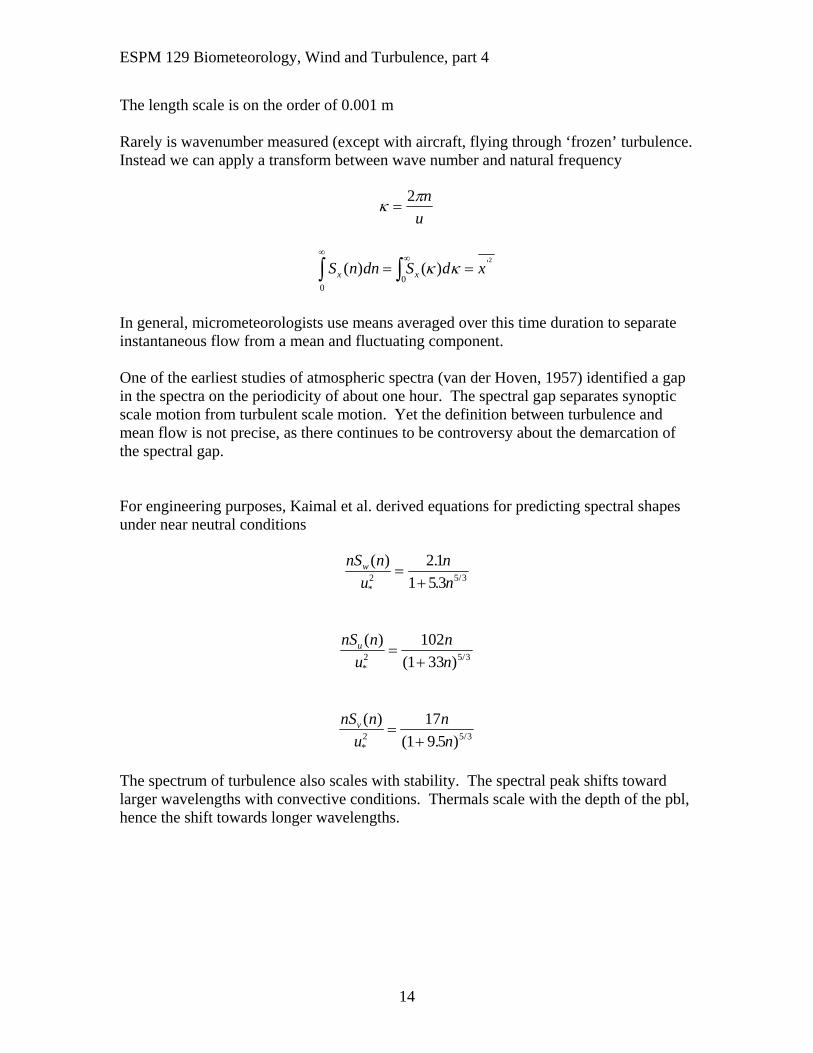
The spectrum of turbulence also scales with stability. The spectral peak shifts toward larger wavelengths with convective conditions. Thermals scale with the depth of the pbl, hence the shift towards longer wavelengths.


15

Figure 7 Computations of Spectra as a function of stability, using the Kaimal functions

Accumulating data taken over tall forests also show evidence of a spectral shift, as compared to idea conditions simulated by the Kaimal spectra.

Widely used set of equations for computing turbulence power spectra and co-

spectra have been developed for a range of turbulence stabilities (Kaimal et al., 1972;

Wyngaard, Cote, 1972). Equation 9 is an example of a cospectra model for the uw

covariance, as a function of z/L:

4/32*

( )( )

1, 2 0( )

1 7.9 , 0 2

uwuw uw

uw

nS n za G f

u L

zz LG

z zL

L L

Equation 1

nz/u

0.0001 0.001 0.01 0.1 1 10 100

nSw

w(n

)/ w

2

0.0001

0.001

0.01

0.1

1

z/L=0 z/L=1 z/L=-1


16

The function Guw depends on z/l and auw is an empirical coefficient. These equations are

based on fewer than 20 hours of turbulence measurements over a flat surface in Kansas.

Recently, they have been revisited and revised by Su et al (2004), using 40000 hours of

turbulence data from over 2 mixed hardwood stands. Both sets of studies show that

spectral peaks shift toward higher wavenumbers, or frequencies, as atmospheric

conditions transcend from unstable to stable. The newer model parameters are better able

to predict the cospectral behavior under a wider range of stable conditions.

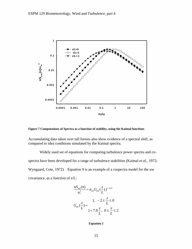
Turbulence Spectra above a forest

Figure 8 Power spectrum of vertical velocity over a temperate deciduous forest

Broad-leaved Forest1.3 h

n/U

0.001 0.01 0.1 1 10

nS

ww(n

)/(w

'w')

0.001

0.01

0.1


17

nS n

u

nn

n

w ( )

. ( )*

max

/2

5 3

2

1 15

nm=0.482+0.437z/L –0.7 <=z/L<=0 Fluxes and Cospectra

The cospectrum gives us information on the spectral distribution of events that contribute the flux density of material. The spectral integral of the co-spectrum equals the flux covariance.

F w r S dc wc w c wc z' ' ( ) 0


18

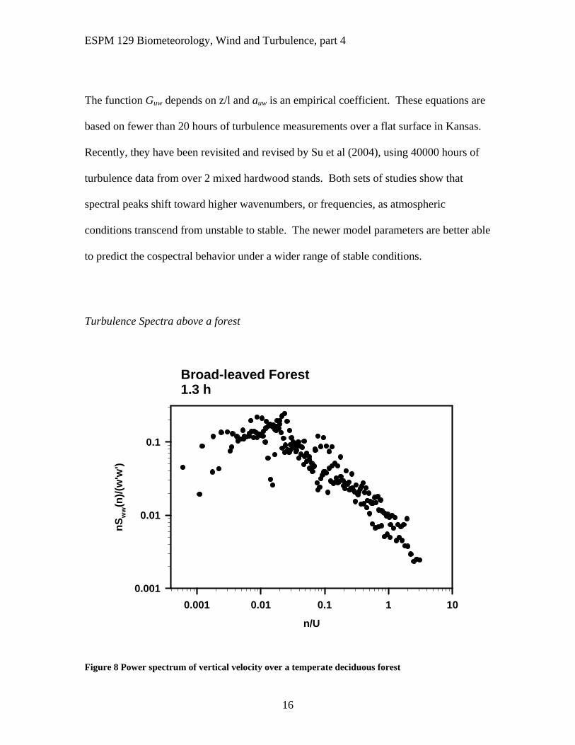
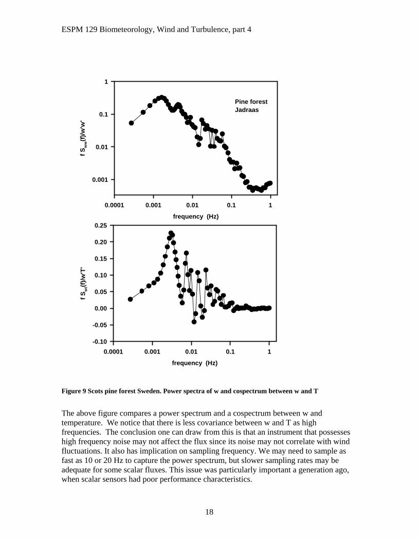
Figure 9 Scots pine forest Sweden. Power spectra of w and cospectrum between w and T

The above figure compares a power spectrum and a cospectrum between w and temperature. We notice that there is less covariance between w and T as high frequencies. The conclusion one can draw from this is that an instrument that possesses high frequency noise may not affect the flux since its noise may not correlate with wind fluctuations. It also has implication on sampling frequency. We may need to sample as fast as 10 or 20 Hz to capture the power spectrum, but slower sampling rates may be adequate for some scalar fluxes. This issue was particularly important a generation ago, when scalar sensors had poor performance characteristics.

Pine forestJadraas

frequency (Hz)

0.0001 0.001 0.01 0.1 1

f S

wt(f

)/w

'T'

-0.10

-0.05

0.00

0.05

0.10

0.15

0.20

0.25

frequency (Hz)

0.0001 0.001 0.01 0.1 1

f S

ww(f

)/w

'w'

0.001

0.01

0.1

1


19

L19.3 Summary: Wind and turbulence in the surface boundary layer many unique and distinct attributes. 1. The mean wind velocity profile experiences greater shear as one approaches the surface. The wind gradient is also a function of diabatic instability. Stronger shear occurs under stable stratification than under unstable stratification. 2. Monin-Obukhov similarity theory is used to define how normalized wind velocity and scalar gradients vary with thermal stratification. The non dimensional height (z/L), as defined by Monin-Obukhov similarity theory is the ratio of buoyant tke to shear produced tke.

3. The wind profile is a logarithmic function of the ratio of height and the surface roughness and is proportional to momentum transfer, quantified in terms of the friction velocity.

4. Turbulence in the surface layer is highly non-Gaussian. It is skewed and kurtotic. Turbulence intensities are on the order of 10 to 20% 5. The turbulence spectra has three characteristic regions, the energy production zone, the inertial subrange and the viscous dissipation range. The spectral peak moves towards longer wavelengths (lower frequencies) under unstable conditions and towards shorter wavelengths (higher frequencies) under stable conditions. 6. Turbulent kinetic energy is produced by shear and buoyancy, it can be transferred into and out of a region and is destroyed by viscous dissipation and is converted into heat. References: Arya, S. P. 1988. Introduction to Micrometeorology. Academic Press. Blackadar, A.K. 197. Turbulence and Diffusion in the Atmosphere, Springer Garratt, J.R. 1992. The Atmospheric Boundary Layer. Cambridge Univ Press. 316 pp. Hogstrom, U. 1996. Review of some basic characteristics of the atmospheric surface layer. Boundary-Layer Meteorology. 78, 2215-246 Hogstrom, U. 1988. Non-dimensional wind and temperature profiles in the atmospheric surface layer, a re-evaluation. Boundary Layer Meteorology. 42, 55-78. Kaimal, J.C. and J.J. Finnigan. 1994. Atmospheric Boundary Layer Flows: Their Structure and Measurement. Oxford Press.


20

Panofsky, H.A. and J.A. Dutton. 1984. Atmospheric Turbulence. Wiley and Sons, 397 pp. Raupach, M.R., R.A. Antonia and S. Rajagopalan. 1991. Rough wall turbulent boundary

layers. Applied Mechanics Reviews. 44, 1-25. Shaw, R. 1995. Lecture Notes, Advanced Short Course on Biometeorology and

Micrometeorology. Stull, R.B. 1988. Introduction to Boundary Layer Meteorology. Reidel Publishing.

Dordrect, The Netherlands. Thom, A (1975). Momentum, Mass and Heat Exchange of Plant Communities. In;

Vegetation and the Atmosphere, vol 1. JL Monteith, ed. Academic Press. Van Gardingen, P. and J. Grace. 1991. Advances in Botanical Research. 18: 189-253. Wyngaard, J.C. 1992. Atmospheric Turbulence Annual. Review of Fluid Mechanics 24:

205-233 Homework problems

1. Using the stability corrected gradient theory and compute wind velocity profiles for neutral (z/L=0), stable, z/L=0.25 and unstable stratification (z/L=-1.5) for cases of u* 0.1, 0.2, 0.3, 0.5 m/s and z=1,3,5,10 m. Assume d is zero and zo is 0.01 m

2. Compute wind velocity profiles for near neutral conditions for a canopy 1, 3 and 10 m tall, using d = 60% and 80% canopy height. Assume zo is 10% of canopy height. Use several values of friction velocity

EndNote References Kaimal JC, Izumi Y, Wyngaard JC, Cote R (1972) Spectral Characteristics of Surface-

Layer Turbulence. Quarterly Journal of the Royal Meteorological Society 98, 563-&.

Stull RB (1988) Introduction to Boundary Layer Meteorology Kluwer, Dordrecht, The Netherlands.

Su H-B, Schmid HP, Grimmond CSB, Vogel CS, Oliphant AJ (2004) Spectral Characteristics and Correction of Long-Term Eddy-Covariance Measurements Over Two Mixed Hardwood Forests in Non-Flat Terrain. Boundary Layer Meteorology 110, 213-253.

Wyngaard JC, Cote OR (1972) Cospectral similarity in the atmospheric surface layer. Quarterly Journal of the Royal Meteorological Society 98, 590-603.


21

Appendix Fourier Transforms Spectrum of turbulence Turbulence is embedded within a continuous spectrum of atmospheric motion, certain attributes must be ascribed to distinguish turbulence from other flow phenomena (e.g. gravity waves, Kelvin Helmholtz waves, Rossby waves). Meteorologists often find it convenient to apply a Fourier transform to a time record of turbulence to examine its spectral properties. The Fourier transform (Sxx()) at a particular angular frequency (=2fradians per second; f is natural frequency; cycles per second) of a stochastic time series (x(t)) is defined as:

F f t i t dtxx ( ) ( ) exp( )

z (1

In Equation 1, i is the imaginary number, i and exp( ) cos sinix x i x is Euler’s function. Fourier transform coefficients can be computed using discrete Fourier transforms The Forward Transform coefficient for a given frequency, n, is a function of the summation of the time series fx.

F nf j

Ni nj Nx

x

j

N

( )( )

exp( / )

0

1

2

F nN

f j nj Ni

Nf j nj Nx x

j

N

xj

N

( ) ( ) cos( / ) ( ) sin( / )

12 2

0

1

0

1

If one knows the Fouier transform coefficients, the original time series can be reconstructed by use of the inverse transform.

f j F n i nj Nx xn

N

( ) ( ) exp( / ) 2

0


22

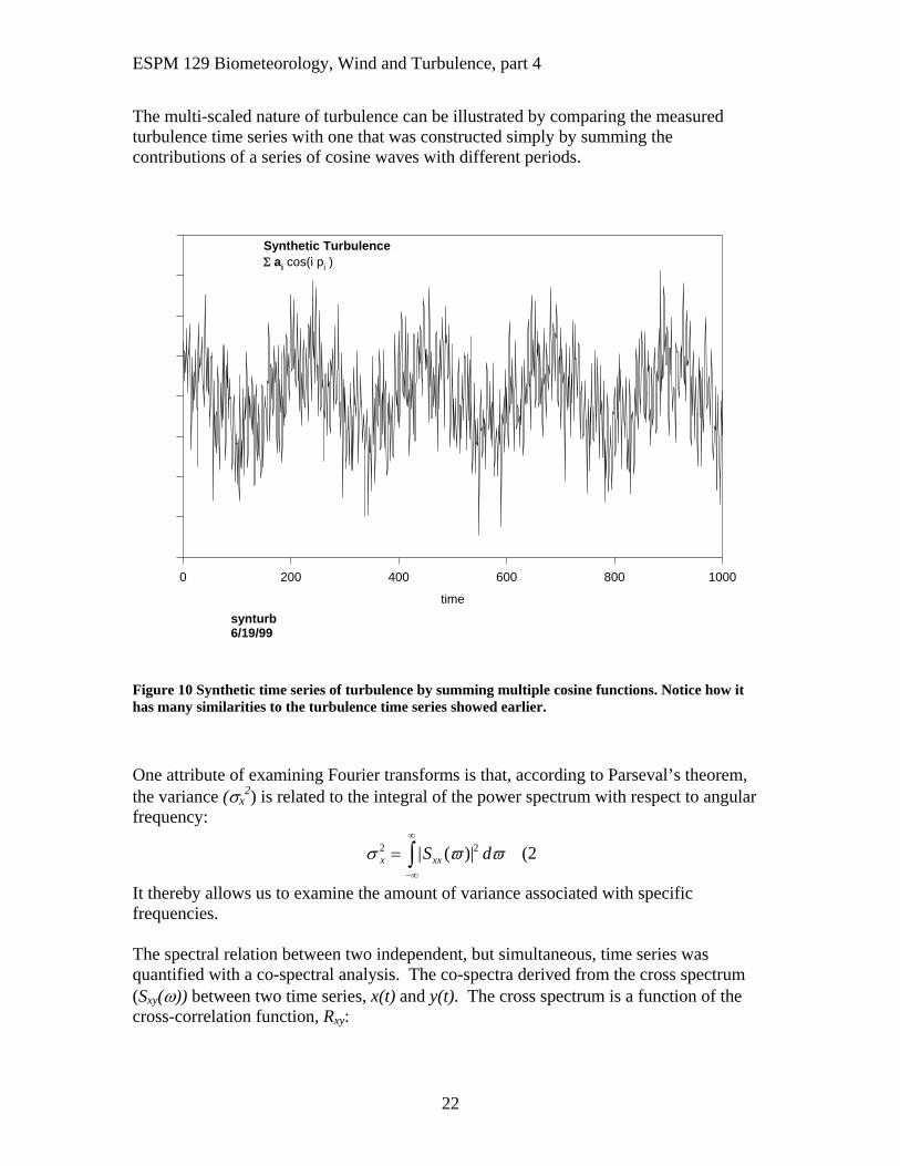
The multi-scaled nature of turbulence can be illustrated by comparing the measured turbulence time series with one that was constructed simply by summing the contributions of a series of cosine waves with different periods.

Figure 10 Synthetic time series of turbulence by summing multiple cosine functions. Notice how it has many similarities to the turbulence time series showed earlier.

One attribute of examining Fourier transforms is that, according to Parseval’s theorem, the variance (x

2) is related to the integral of the power spectrum with respect to angular frequency:

x xxS d2 2

z | ( )| (2

It thereby allows us to examine the amount of variance associated with specific frequencies. The spectral relation between two independent, but simultaneous, time series was quantified with a co-spectral analysis. The co-spectra derived from the cross spectrum (Sxy()) between two time series, x(t) and y(t). The cross spectrum is a function of the cross-correlation function, Rxy:

Synthetic Turbulenceai cos(i pi )

time

0 200 400 600 800 1000

synturb6/19/99


23

S R i dxy xy( ) ( ) exp( )

z1 (3

The cross-correlation between x(t) and y(t+) is computed as:

R TT

x t y t dtxy

T

T

z( ) ( ) ( )lim 1

2 (4

The cross-spectrum has an even and odd component:

S Co iQxy xy xy( ) ( ) ( ) (5

The even component of the cross spectrum yields the co-spectrum, Coxy()):

Co R dxy xy( ) ( ) cos( )

z1 (6

and the odd component yields the quadrature, Qxy()), spectrum:

Q R dxy xy( ) ( ) sin( )

z1 (7

The mean covariance equals the integral of the co-spectrum from minus to plus infinity and is proportional to the mean eddy flux density. The phase angle between two signals is, subsequently, computed as:

tan( )

( )

Q

Coxy

xy

(8

The Fast Fourier method (Carter and Ferrier, 1979; Hamming, Press et al. 1992) was used to compute power spectra, co-spectra and phase angle spectra. Fundamentally, these calculations are performed on discrete and evenly-spaced, time series. The specific frequencies that can be decomposed from such a time series are defined fromf n N tn / ( ) , where the time step between samples is t , the total number of samples

is denoted as N and the index n varies from –N/2 to +N/2. The discrete Fourier transform (Fx) for for a time series (f(n)) at a time index number k is:

F k f n i nk Nxn

N

( ) ( ) exp( )

20

1

(9

The power spectrum is a function of the Fourier transform and its complex conjugate

S kt

NF k F kx x x( ) ( ) ( )*

. The co-spectrum and quadrature spectrum between two


24

variables, x and y, are computed in a related manner, with respect to the real (

Co kt

NF k F kxy x y( ) Re( ( ) ( ))*

) and imaginary ( Q k

t

NF k F kxy x y( ) Im( ( ) ( ))*

)

components.

lecture 19 wind and turbulence part 4 surface boundary ... · espm 129 biometeorology, wind and...

Documents