lecture 3 - university of arizona
TRANSCRIPT

Lecture 3
Frits Beukers
Arithmetic of values of E- and G-function
Lecture 3 E- and G-functions 1 / 20
G-functions, definition
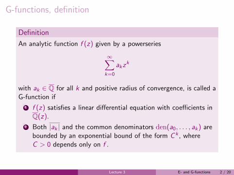
Definition
An analytic function f (z) given by a powerseries
∞∑k=0
akzk
with ak ∈ Q for all k and positive radius of convergence, is called aG-function if
1 f (z) satisfies a linear differential equation with coefficients inQ(z).
2 Both |ak | and the common denominators den(a0, . . . , ak) arebounded by an exponential bound of the form C k , whereC > 0 depends only on f .
Lecture 3 E- and G-functions 2 / 20
G-functions, examples
1 f (z) is algebraic over Q(z) (Eisenstein theorem).
2
f (z) = 2F1
(α, β
γ
∣∣∣∣ z
)Gauss hypergeometric series with α, β, γ ∈ Q.
3 f (z) = Lk(z) =∑
n≥1zn
nk , the k-th polylogarithm.
4 f (z) =∑∞
k=0 akzk wherea0 = 1, a1 = 3, a2 = 19, a3 = 147, . . . are the Apery numberscorresponding to Apery’s irrationality proof of ζ(2). They aredetermined by
ak =k∑
r=0
(k
r
)2(r + k
r
)and satisfy the recurrence relation(n + 1)2an+1 = (11n2 − 11n + 3)an − n2an−1.
Lecture 3 E- and G-functions 3 / 20
Periods
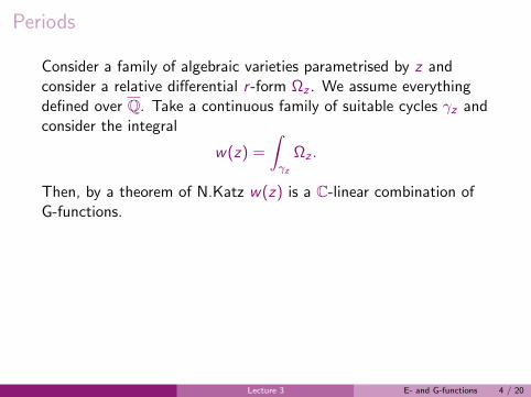
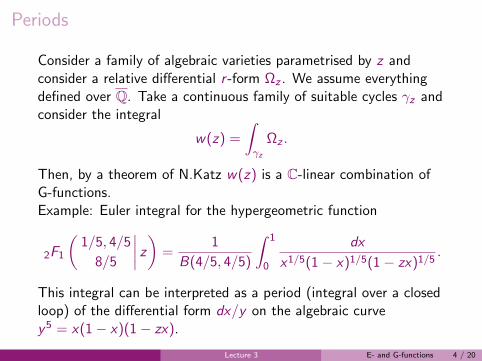
Consider a family of algebraic varieties parametrised by z andconsider a relative differential r -form Ωz . We assume everythingdefined over Q. Take a continuous family of suitable cycles γz andconsider the integral
w(z) =
∫γz
Ωz .
Then, by a theorem of N.Katz w(z) is a C-linear combination ofG-functions.
Example: Euler integral for the hypergeometric function
2F1
(1/5, 4/5
8/5
∣∣∣∣ z
)=
1
B(4/5, 4/5)
∫ 1
0
dx
x1/5(1− x)1/5(1− zx)1/5.
This integral can be interpreted as a period (integral over a closedloop) of the differential form dx/y on the algebraic curvey5 = x(1− x)(1− zx).
Lecture 3 E- and G-functions 4 / 20
Periods
Consider a family of algebraic varieties parametrised by z andconsider a relative differential r -form Ωz . We assume everythingdefined over Q. Take a continuous family of suitable cycles γz andconsider the integral
w(z) =
∫γz
Ωz .
Then, by a theorem of N.Katz w(z) is a C-linear combination ofG-functions.Example: Euler integral for the hypergeometric function
2F1
(1/5, 4/5
8/5
∣∣∣∣ z
)=
1
B(4/5, 4/5)
∫ 1
0
dx
x1/5(1− x)1/5(1− zx)1/5.
This integral can be interpreted as a period (integral over a closedloop) of the differential form dx/y on the algebraic curvey5 = x(1− x)(1− zx).
Lecture 3 E- and G-functions 4 / 20

Irrationality results
A typical result for G-functions,
Galochkin, 1972
Let (f1(z), . . . , fn(z)) be a solution vector of a system of first orderequations of the form y′ = Gy and suppose that the fi (z) areG-functions with coefficients in Q. Suppose also thatf1(z), . . . , fn(z) are linearly independent over Q(z) and that thesystem satisfies the so-called Galochkin condition. Then thereexists C > 0 such that f1(a/b), . . . , fn(a/b) are Q-linearindependent whenever a, b ∈ Z and b > C |a|n+1 > 0.
Lecture 3 E- and G-functions 5 / 20

Wolfart’s examples
Theorem, Wolfart 1988
The functions 2F1
(1/12, 5/12
1/2
∣∣∣ z)
and 2F1
(1/12, 7/12
2/3
∣∣∣ z)
assume
algebraic values for a dense set of algebraic arguments in the unitdisk.
Theorem, Wolfart+FB, 1989
We have
2F1
(1
12,
5
12,1
2
∣∣∣∣ 1323
1331
)=
3
44√
11.
2F1
(1
12,
7
12,2
3
∣∣∣∣ 64000
64009
)=
2
36√
253.
Lecture 3 E- and G-functions 6 / 20

Galochkin condition
Start with the systemy′ = Gy
For s = 1, 2, 3, . . . define the iterated n × n-matrices Gs by
1
s!y(s) = Gsy.
Let T (z) be the common denominator of all entries of G . Then,for every s, the entries of T (z)sGs are polynomials. Denote theleast common denominator of all coefficients of all entries ofT (z)mGm/m! (m = 1, . . . , s) by qs .
Definition
With notation as above, we say that the system y′(z) = G (z)y(z)satisfies Galochkin’s condition if there exists C > 0 such thatqs < C s for all s ≥ 1.
Lecture 3 E- and G-functions 7 / 20

Why Galochkin’s condition?
Recall that in Siegel’s method we construct polynomials Pi ofdegree ≤ N such that
P1f1 + · · ·+ Pnfn = O(zN(n−ε)).
In vector notation P · f = O(zN(n−ε)). We also need the derivatives
1
m!(P · f)(m) = O(zN(n−ε)−m), m = 0, 1, . . . ,Nε + γ.
Notice
1
m!(P · f)(m) =
m∑s=0
1
s!(m − s)!(P)(m−s) · (f)(s)
=m∑
s=0
1
(m − s)!(P)(m−s) · Gs f
Lecture 3 E- and G-functions 8 / 20

Galochkin implies G-property
Lemma
Suppose we have an n × n-system satisfying Galochkin. Then, atany nonsingular point a the system has a basis of solutionsconsisting of G-functions in z − a.
Proof Put G0 equal to the n × n identity matrix and consider thematrix
Y =∑s≥0
1
s!Gs(a)(z − a)s .
It satisfiesY ′ = GY
hence its columns satisfy the linear differential system and sincedet(Y ) 6= 0 they form a basis. The G-function property ofGs(a)/s! follows directly from Galochkin’s condition.
Lecture 3 E- and G-functions 9 / 20

Chudnovsky’s theorem
Chudnovsky, 1984
Let (f1(z), . . . , fn(z)) be a solution vector consisting of G-functionsof a system of first order equations of the form y′ = Gy. Supposethat f1(z), . . . , fn(z) are linearly independent over Q(z). Then thesystem satisfies Galochkin’s condition.
Idea of proof: Construct Q,P1, . . . ,Pn ∈ Q[z ] of degrees ≤ N suchthat
Qfi − Pi = O(zN(1+1/n−ε)).
In vector notation:
Qf − P = O(zN(1+1/n−ε)).
Differentiate,
Q ′f + Qf ′ − P′ = O(zN(1+1/n−ε)−1).
Lecture 3 E- and G-functions 10 / 20

Proof sketch of Chudnovsky’s theorem
Use f ′ = G f to get
Q ′f + QG f − DP = O(zN(1+1/n−ε)−1)
where P′ = DP.
Substract G times the original form
Q ′f − (D − G )P = O(zN(1+1/n−ε)−1).
Repeating the argument s times and divide by s!,
1
s!Q(s)f − 1
s!(D − G )sP = O(zN(1+1/n−ε)−s).
Lemma
We have for any vector P ∈ Q(z)n,
GsP =s∑
m=0
(−1)m
(s −m)!m!Ds−m(D − G )mP.
Lecture 3 E- and G-functions 11 / 20

Proof sketch of Chudnovsky’s theorem
Use f ′ = G f to get
Q ′f + QG f − DP = O(zN(1+1/n−ε)−1)
where P′ = DP.Substract G times the original form
Q ′f − (D − G )P = O(zN(1+1/n−ε)−1).
Repeating the argument s times and divide by s!,
1
s!Q(s)f − 1
s!(D − G )sP = O(zN(1+1/n−ε)−s).
Lemma
We have for any vector P ∈ Q(z)n,
GsP =s∑
m=0
(−1)m
(s −m)!m!Ds−m(D − G )mP.
Lecture 3 E- and G-functions 11 / 20

Galochkin’s condition for equations
Consider the differential
T (z)y (n) = Qn−1(z)y (n−1) + · · ·+ Q1(z)y ′ + Q0y
where T (z),Q0(z), . . . ,Qn−1(z) are polynomials in Q[z ].
By recursion on m find polynomials Qm,r ∈ Q(z) forr = 0, 1, . . . , n − 1 such that
T (z)m−n+1y (m) = Qm,n−1(z)y (n−1) + · · ·+ Qm,1(z)y ′ + Qm,0(z)y .
In particular Qn,r (z) = Qr (z).
Definition
The equation satisfies Galoschkin’s condition if there exists C > 0such that for every integer s the common denominator of allcoefficients of all polynomials 1
m!Qm,r withn ≤ m ≤ s, 0 ≤ r ≤ n − 1 is bounded by C s .
Lecture 3 E- and G-functions 12 / 20

Galochkin’s condition for equations
Consider the differential
T (z)y (n) = Qn−1(z)y (n−1) + · · ·+ Q1(z)y ′ + Q0y
where T (z),Q0(z), . . . ,Qn−1(z) are polynomials in Q[z ].By recursion on m find polynomials Qm,r ∈ Q(z) forr = 0, 1, . . . , n − 1 such that
T (z)m−n+1y (m) = Qm,n−1(z)y (n−1) + · · ·+ Qm,1(z)y ′ + Qm,0(z)y .
In particular Qn,r (z) = Qr (z).
Definition
The equation satisfies Galoschkin’s condition if there exists C > 0such that for every integer s the common denominator of allcoefficients of all polynomials 1
m!Qm,r withn ≤ m ≤ s, 0 ≤ r ≤ n − 1 is bounded by C s .
Lecture 3 E- and G-functions 12 / 20

Chudnovski’s Theorem, bis
Theorem, Chudnovsky 1984
Let f be a G-function and let Ly = 0 be its minimal differentialequation. Then Ly = 0 satisfies Galochkin’s condition.
Lecture 3 E- and G-functions 13 / 20

Regular singularities
Consider a linear differential equation
pny(n) + pn−1y
(n−1) + · · ·+ p1y′ + p0y = 0
where pi ∈ C[z ] for all i . Suppose that pn(0) = 0. Then z = 0 is asingular point.
Criterion for regular singular points
The point z = 0 is regular or a regular singular point if and only ifthe pole order of pi/pn at z = 0 is at most n − i .
Alternative criterion
The point z = 0 is regular or a regular singular point if and only ifthe equation can be rewritten as
znqny(n) + zn−1qn−1y
(n−1) + · · ·+ zq1y′ + q0y = 0
where qi ∈ C[z ] and qn(0) 6= 0.
Lecture 3 E- and G-functions 14 / 20

Regular singularities
Consider a linear differential equation
pny(n) + pn−1y
(n−1) + · · ·+ p1y′ + p0y = 0
where pi ∈ C[z ] for all i . Suppose that pn(0) = 0. Then z = 0 is asingular point.
Criterion for regular singular points
The point z = 0 is regular or a regular singular point if and only ifthe pole order of pi/pn at z = 0 is at most n − i .
Alternative criterion
The point z = 0 is regular or a regular singular point if and only ifthe equation can be rewritten as
znqny(n) + zn−1qn−1y
(n−1) + · · ·+ zq1y′ + q0y = 0
where qi ∈ C[z ] and qn(0) 6= 0.Lecture 3 E- and G-functions 14 / 20

Regular singularities in general
Consider a differential equation
pny(n) + pn−1y
(n−1) + · · ·+ p1y′ + p0y = 0
with pi ∈ Q[z ] and let a be any point in C ∪∞.
Rewrite the equation in terms of a local parameter t at a(which comes down to putting z = t + a and z = 1/t ifa = ∞).
If t = 0 is a regular singularity of the resulting equation, wesay that a is a regular singularity of the orginal equation.
Proposition
The point z = ∞ is a singular point if and only ifdeg(pi ) ≤ deg(pn)− n + i for i = 0, 1, . . . , n
Lecture 3 E- and G-functions 15 / 20
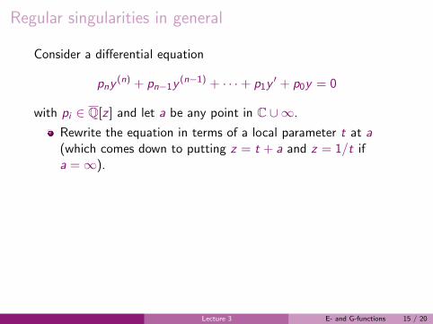
Fuchsian equations
Definition
A linear differential equation is called Fuchsian if every point inC ∪∞ is regular or a regular singularity.
Example: y ′ = y is not a Fuchsian equation because ∞ is not aregular singularity (Replace z = 1/t and we obtain −t2 dy
dt = y).
Lecture 3 E- and G-functions 16 / 20
Galochkin implies Fuchsian
Theorem
Suppose the differential equation Ly = 0 satisfies Galochkin’scondition. Then Ly = 0 is Fuchsian.
For the experts: Galochkin’s condition implies that the equation isglobally nilpotent (Bombieri,Dwork). That is
Dsp ≡ M L (mod p)
for almost all primes p and some integer s.N.Katz showed that a globally nilpotent equation is Fuchsian withrational local exponents.
Lecture 3 E- and G-functions 17 / 20

Galochkin to Fuchsian, proof sketch
By way of example consider the equation
z2y ′′ = zA1y′ + A0y
where A1,A0 are rational functions.
Suppose the equation is not Fuchsian. By way of example assumethat A1,A0 both have a first order pole in z = 0.By induction on m,
zmy (m) = zAm,1y′ + Am,0y
and
Am+1,1 = (1−m)Am,1 + zA′m,1 + Am,1A1 + Am,0
Am+1,0 = Am,1A0 + zA′m,0 −mAm,0
Lecture 3 E- and G-functions 18 / 20

Galochkin to Fuchsian, proof sketch
By way of example consider the equation
z2y ′′ = zA1y′ + A0y
where A1,A0 are rational functions.Suppose the equation is not Fuchsian. By way of example assumethat A1,A0 both have a first order pole in z = 0.
By induction on m,
zmy (m) = zAm,1y′ + Am,0y
and
Am+1,1 = (1−m)Am,1 + zA′m,1 + Am,1A1 + Am,0
Am+1,0 = Am,1A0 + zA′m,0 −mAm,0
Lecture 3 E- and G-functions 18 / 20

Galochkin to Fuchsian, proof sketch
By way of example consider the equation
z2y ′′ = zA1y′ + A0y
where A1,A0 are rational functions.Suppose the equation is not Fuchsian. By way of example assumethat A1,A0 both have a first order pole in z = 0.By induction on m,
zmy (m) = zAm,1y′ + Am,0y
and
Am+1,1 = (1−m)Am,1 + zA′m,1 + Am,1A1 + Am,0
Am+1,0 = Am,1A0 + zA′m,0 −mAm,0
Lecture 3 E- and G-functions 18 / 20

Galochkin to Fuchsian, continued
From the previous slide,
z2y ′′ = zA1y′ + A0y
and that A1,A0 have pole order 1. By induction,
zmy (m) = zAm,1y′ + Am,0y
Suppose residue of A1 at z = 0 is a. Then
Am,1 =am−1
zm−1+ · · ·
So Am,1 is a rational function whose numerator has a constantterm which grows exponentially in m. Thus Am,1/m! cannotsatisfy Galochkin’s condition.
Lecture 3 E- and G-functions 19 / 20

Chudnovski’s Theorem, encore
Theorem, Chudnovsky 1984
Let f be a G-function and let Ly = 0 be its minimal differentialequation. Then Ly = 0 satisfies Galochkin’s condition.
Moreover, z = 0 is at worst a regular singularity of Ly = 0
Lecture 3 E- and G-functions 20 / 20

Chudnovski’s Theorem, encore
Theorem, Chudnovsky 1984
Let f be a G-function and let Ly = 0 be its minimal differentialequation. Then Ly = 0 satisfies Galochkin’s condition.Moreover, z = 0 is at worst a regular singularity of Ly = 0
Lecture 3 E- and G-functions 20 / 20