SSGection

tatistical

enetics

ON

Department of Biostatistics

School of Public Health

Grier P Page, Ph.D.Associate Professor

Quality Control of Microarray Studies

Microarrays

From Affymetrix.com

www.biology.ucsc.edu/ mcd/research.html

Quality Control In Microarray Studies

Which one is good or bad?

One view of the steps for a microarray study

But essentially no quality checking of the data

From Drug Discov Today. 2005 Sep 1;10(17):1175-82.

The Myth That Data Mining has No Hypothesis

• There always needs to be a biological question in the experiment. If there is not even a question don’t bother.

• The question could be nebulous: What happens to the gene expression of this tissue when I apply Drug A.

• The purpose of the question is to drive the experimental design.

• Make sure the samples answer the question: Cause vs. effect.

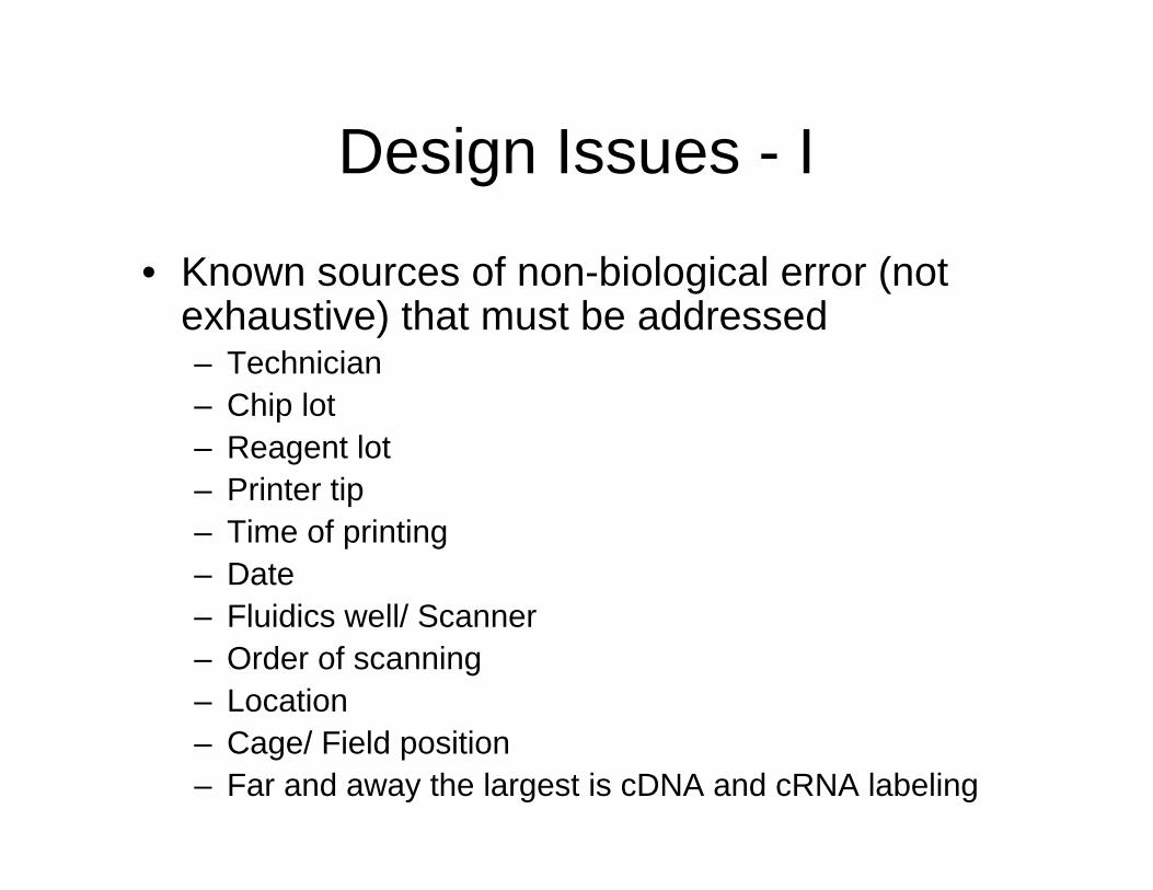
Design Issues - I

• Known sources of non-biological error (not exhaustive) that must be addressed– Technician– Chip lot– Reagent lot– Printer tip– Time of printing– Date– Fluidics well/ Scanner– Order of scanning– Location– Cage/ Field position – Far and away the largest is cDNA and cRNA labeling

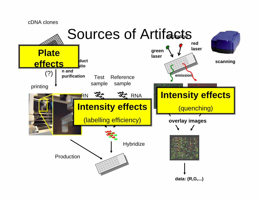
Sources of Artifacts

scanning

data: (R,G,...)

cDNA clones

PCR product amplification and purification

printing

Hybridize

RNA

Testsample

cDNA

RNA

Reference sample

cDNA

excitationred lasergreen

laser

emission

overlay images

Production

Plateeffects

(?)

Intensity effects(labelling efficiency)

Intensity effects(quenching)

UMSA Analysis

Insulin Resistant

Insulin Sensitive

Day 1Day 2

Example of Day or Batch Effect

• PCA of muscle dataMean vs. Variance by Chip

0

100

200

300

400

500

600

700

800

0.E+00 1.E+06 2.E+06 3.E+06 4.E+06 5.E+06 6.E+06Variance of Intensity

Ave

rage

Inte

nsity

Phase1 U95APhase 2 U95APhase 3 U95A

Design Issues – II• How to address these issues

– Make the experiment as uniform as possible• Agree on exactly what defines the tissue to be used, use

same technician, same chip lot, same reagents (always buy a little too much), same scanner, do sample extraction, labeling and hybridization on one day if possible, establish quality control

– Randomize when uniformity is not possible• Don’t do all of condition 1 on day 1 and condition 2 on day 2• Randomize the time a chips sits waiting to be scanned• Randomize animal cage/plant field position

• Microarrays generate such a huge volume of data that is is possible to detect these issues, I suspect that northerns, Southerns, RT-PCR, westerns, and more have similar problems.

What is Orthogonalization vsRandomization ?

• Orthogonalization- spreading the biological sources of error evenly across the non-biological sources of error. – Maximally powerful for known sources of

error.• Randomization – spear the biological

sources of error at random across the non-biological sources of error.– Useful for controlling for unknown sources of

error

Examples of Orthogonalizationand Randomization ?

228127226125214113212111VarietyTreatmentSample #

3847768564532211SampleOrder

3857862514436271SampleOrder

The experiment Orthogonalize Randomize

RNA Quality

Quality control of RNA• Confirmation of RNA

integrity, based on an 28S:18S ratio greater than 1.5 as quantified by Agilent BioAnalyzer and formaldehyde gel electrophoresis

• However, • The Drosophila RNA has

a split peak for the 28s ribosomal RNA on theBioanalyzer.

Intact RNA

Degraded RNA

Images from Agilent

Be aware of what your specific Species should look like

• The Drosophila RNA has a split peak for the 28s ribosomal RNA on the Bioanalyzer.

• And no 18S peak

Affymetrix QC metrics• The average background is calculated from the 2% probes with the

weakest signal. The average background is an estimate of generalnonspecific binding based on low-intensity features across an array.

• Bio B isa probe set designed to measure prelabeled bacterial nucleotides. Bio B is the signal from internal prelabeled standards and measures the efficacy of hybridization, washing, and scanning. Bio B is free of RNA, amplification, and labeling effects.

• The actin 3/5 ratio is a ratio of probe sets designed to detect the 3 and 5 regions of the actin mRNA transcript and is reputed to detect RNA degradation. This ratio is thought to indicate RNA quality a well as the bias inherent in the Affymetrix labeling assay.

• The scale factor is a global normalization constant based on the trimmed mean of probe set signals or average differences and is inversely related to chip brightness.

• Percent present is an array level summary of the results of a statistical function designed to predict the presence or absence of each transcript. Percent present is a quality metric that is sensitive to any error source from RNA sampling to scanning and data extraction. Percent present is influenced by all stages in the microarray process including scanner brightness, background, RNA quality, algorithm, and chip design.

Relationship among metrics

From Finkelstein . Mol Methods xxx

RNA digestion plot

5' <-----> 3' Probe Number

Mea

n In

tens

ity :

shift

ed a

nd s

cale

d

0 2 4 6 8 10

020

4060

Does one size fit all?

The red/green ratios can be spatially biased

• .Top 2.5%of ratios red, bottom 2.5% of ratios green

Spatial plots: background from the two slides

Image and Data Quality Checking

X

Y

An illustration of principle of a geography index: A full polynomial model is used to detect spatial patterns (e.g. upper right corner).

Geography index (GEODEX). A full polynomial model was used to detect spatial patterns: z = x + y + x2 + xy + y2 + x3 + x2y + xy2 + y3 + xy3 + x2y2 + x3y + x2y3 + x3y2 + x3y3, where z – expression level and x & y – Cartesian coordinates of an array. Foreground and background readings for each channel were processed separately. Geography indices were determined as follows: GEODEX = 1 - R2, where R2 is a coefficient of determination for a polynomial model.

Distribution of the geography index (GEODEX) for individual chips

0.95

0.96

0.97

0.98

0.99

1

1 3 5 7 9 11 13 15 17 19 21 23 25

Chip ID

GEO

DEX

Image of the right corner on the bottom.

Image of chip 12

A. Foreground - high GEODEX values C. Background - high GEODEX values

B. Foreground - low GEODEX values D. Background - low GEODEX values

X-axis and Y-axis - Cartesian coordinates of an array; Z-axis - foreground or background signal readings.

In this analysis lower GEODEX is considered a worse outcome.

These are OK

These are not OK

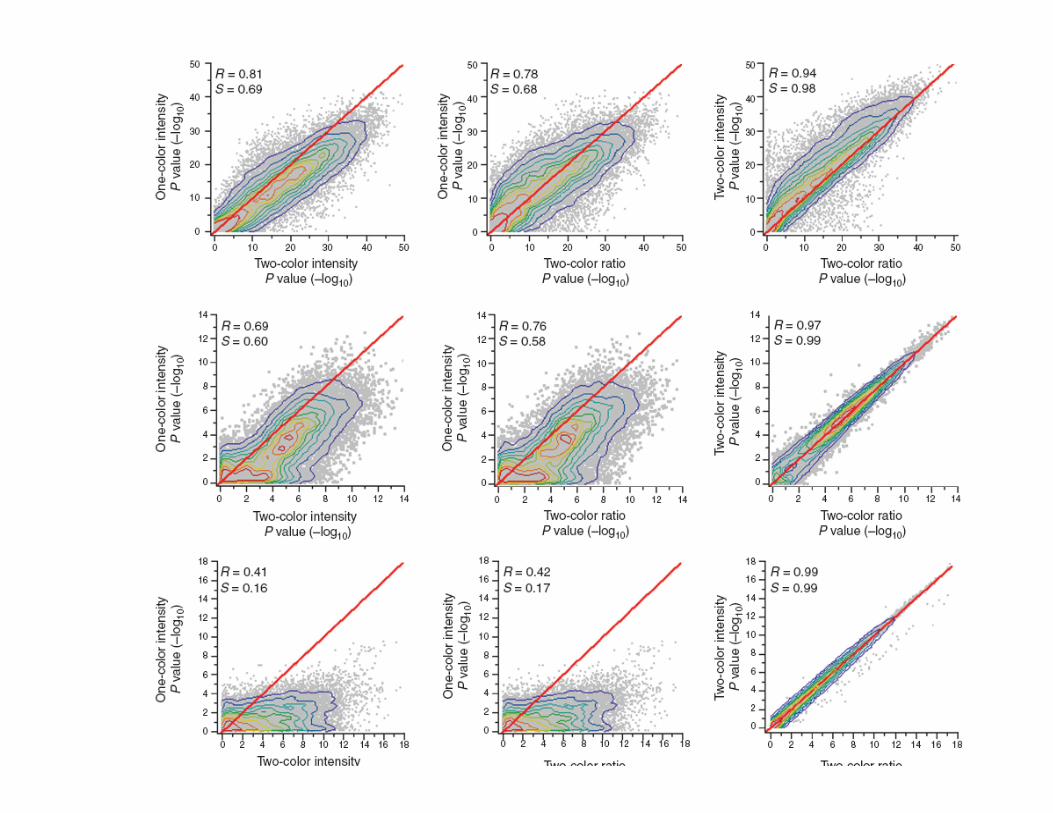
Quality Control Using Deleted Residuals

Page GP, Edwards JW, Yelisetti P, & Allison DB Assessing Qualityof Microarrays Using Studentized Deleted Residuals using normative data from 4358 arrays from a public database. In preparation

Using Deleted Residual Plots & Statistics to Assess Array Quality

• Traditional tools for detecting outliers do not work when n is small.

• Deleted residuals can work when n is small.• Within a single gene, the distribution of the deleted

residuals is t with n-2 degrees of freedom.• By looking at all the genes on a chip, we may be able to

use apparent departure from tn-2 among the deleted residuals as a measure of array quality.

• Compare are the observed deleted residuals to the expected t with a Kolmogorov-Smirnov test with genes-1 df.

Presumed Good Chip

Presumed Bad Chip

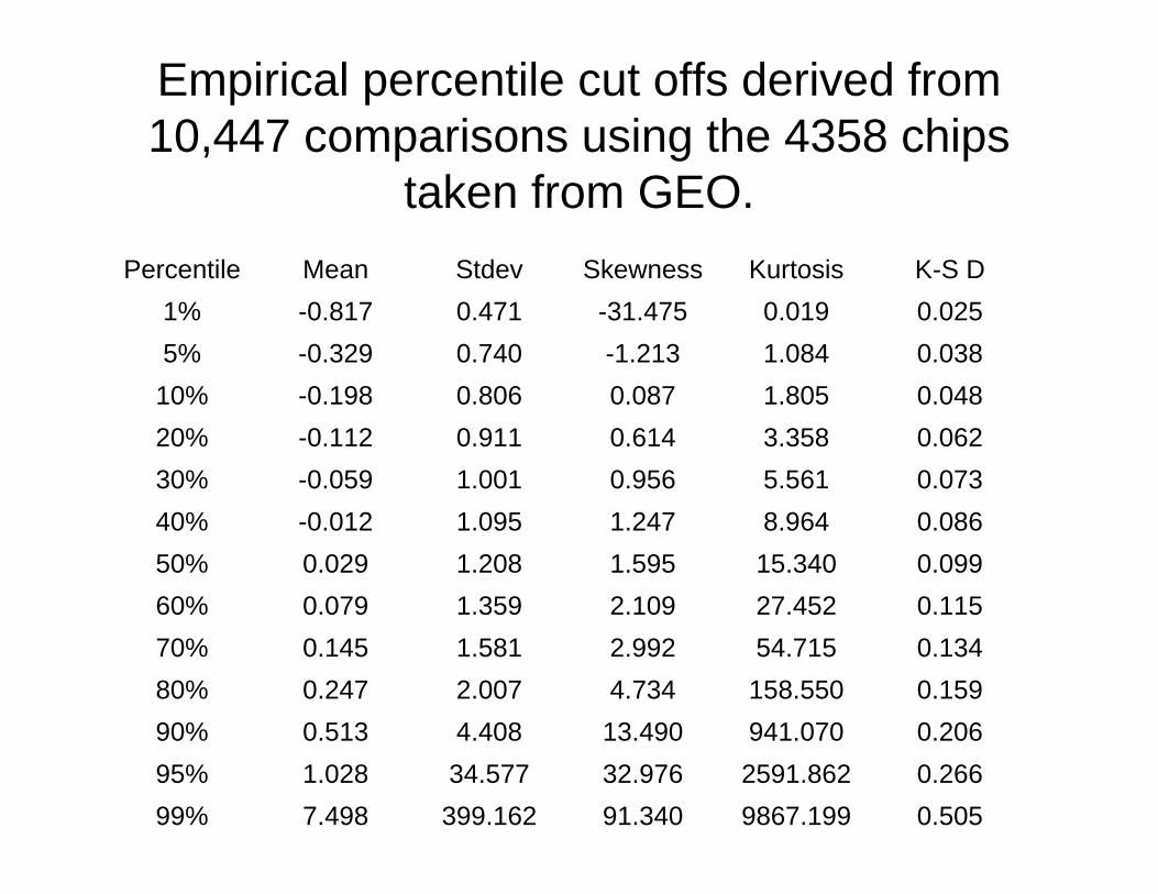
Empirical percentile cut offs derived from 10,447 comparisons using the 4358 chips

taken from GEO.

0.5059867.19991.340399.1627.49899%0.2662591.86232.97634.5771.02895%0.206941.07013.4904.4080.51390%0.159158.5504.7342.0070.24780%0.13454.7152.9921.5810.14570%0.11527.4522.1091.3590.07960%0.09915.3401.5951.2080.02950%0.0868.9641.2471.095-0.01240%0.0735.5610.9561.001-0.05930%0.0623.3580.6140.911-0.11220%0.0481.8050.0870.806-0.19810%0.0381.084-1.2130.740-0.3295%0.0250.019-31.4750.471-0.8171%K-S DKurtosisSkewnessStdevMeanPercentile

Histogram of p-values

Potentially Bad Chip

Histogram of p-values with bad chip removed

Quality Control in Data sources

Understand What Databases Include, don’t include, and assumptions

• Just because a database says something does not mean it is right. Read the evidence.

• Databases are biased. • Databases are incomplete• Databases have lots of data• Understand data before you use it

159550

85

TCA cycle from Ingenuity

TCA from GeneMAPP

TCA cycle from Ingenuity

Issues in the Annotation of Genes

Gene Symbol p-value fc 50/21 Gene Ontology Biological Process Gene Ontology Cellular ComponentPathwayAco2 0.746656 0.955755 --- --- Krebs-TCA_Cycle // Pdk2 0.967577 1.005459 6086 // acetyl-CoA biosynthesis from pyru5739 // mitochondrion // Krebs-TCA_Cycle // Pdk2 0.823635 1.02781 6086 // acetyl-CoA biosynthesis from pyru5739 // mitochondrion // Krebs-TCA_Cycle // Pdha2 0.368075 1.403263 6096 // glycolysis 5739 // mitochondrion Krebs-TCA_Cycle // Idh1 0.710704 0.994378 6099 // tricarboxylic acid cycle 5829 // cytosol ---Acly 0.367315 0.982691 6099 // tricarboxylic acid cycle 5622 // intracellular Fatty_Acid_SynthesAco2 1.22E-06 0.561041 --- --- Krebs-TCA_Cycle // Fh1 6.76E-06 0.690515 6099 // tricarboxylic acid cycle // 5739 // mitochondrion Krebs-TCA_Cycle // Atp5g3 1.53E-06 0.754735 6099 // tricarboxylic acid cycle // 5739 // mitochondrion ---Suclg1 8.87E-07 0.694384 6099 // tricarboxylic acid cycle // 5739 // mitochondrion Krebs-TCA_Cycle // Mdh1 5.92E-09 0.519311 6099 // tricarboxylic acid cycle // --- Krebs-TCA_Cycle // Mor1 4.24E-07 0.617645 6099 // tricarboxylic acid cycle // 5739 // mitochondrion Krebs-TCA_Cycle // Idh1 2.36E-06 0.677013 6099 // tricarboxylic acid cycle // 5829 // cytosol // ---Idh3g 2.19E-06 0.709971 6099 // tricarboxylic acid cycle // 5739 // mitochondrion Krebs-TCA_Cycle // Dlst 2.49E-07 0.688339 --- --- ---Sdhd 5.13E-07 0.583485 6121 // mitochondrial electron transport, s5749 // respiratory chain complex I Krebs-TCA_Cycle // Sdhc 1.82E-06 0.64108 --- --- ---RGD:735073 2.13E-07 0.570307 --- 9352 // dihydrolipoyl dehydrogenas ---Cs 1.56E-07 0.560436 --- 5739 // mitochondrion Krebs-TCA_Cycle // RGD:621624 1E-06 0.486736 6099 // tricarboxylic acid cycle // 5829 // cytosol ---Idh3B 2.57E-07 0.694389 --- --- Krebs-TCA_Cycle // Mdh1 1.08E-05 0.496911 6099 // tricarboxylic acid cycle // --- Krebs-TCA_Cycle // Pc 1.91E-05 0.468765 6094 // gluconeogenesis // 5739 // mitochondrion Krebs-TCA_Cycle // RGD:708561 0.004002 0.76777 --- 5913 // cell-cell adherens junction Krebs-TCA_Cycle // RGD:708561 0.03978 0.686511 --- 5913 // cell-cell adherens junction Krebs-TCA_Cycle // Dlat 4.76E-06 0.435534 6086 // acetyl-CoA biosynthesis from pyru5739 // mitochondrion // Krebs-TCA_Cycle // Sdhd 1.3E-06 0.64335 6121 // mitochondrial electron transport, s5749 // respiratory chain complex I Krebs-TCA_Cycle // Sdha 7.85E-06 0.730667 6099 // tricarboxylic acid cycle // 5739 // mitochondrion // Krebs-TCA_Cycle // Idh3a 0.000449 0.690147 6099 // tricarboxylic acid cycle // 5739 // mitochondrion // Krebs-TCA_Cycle // Pdk4 0.044616 1.700116 6086 // acetyl-CoA biosynthesis from pyru5739 // mitochondrion // Krebs-TCA_Cycle // Cs 1.36E-06 0.592128 --- 5739 // mitochondrion // Krebs-TCA_Cycle // Acly 0.000227 0.554459 6085 // acetyl-CoA biosynthesis 5622 // intracellular // Fatty_Acid_Synthes

Annotation is inconsistent across sources

Nucleic Acids Research, 2005, Vol. 33, No. 3 e31

Nucleic Acids Research, 2005, Vol. 33, No. 3 e31

Nucleic Acids Research, 2005, Vol. 33, No. 3 e31

11749302800584124Many-VendorOne-Blast

368652140836134802353896338One-VendorMany-Blast

18000000Absent-VendorPresent-Blast

1095214972990200823352062930850Present-VendorAbsent-Blast

6413*99791955114788261382435220193

6932

Exact Match

2823282329692969936936250141Nil Entries from vendor(No Mapping for these

probes)

19108191082457624576299542995422810

8297

Vendor Mapping Numbers

AFGC(98%)AFGC(75%)CATMA(98%)CATMA(75%)Operon(98%)Operon(75%)ATH1AG

Mapping of Plant Arrays

MAQC – Nature Biotechnololgy Oct 2006

Summary

• Design your experiment well• Control for non-biological sources of error• Know what is good and bad quality data at

each stage including RNA, image, data, and annotation

• If you are aware of these issues and control for them highly powerful and reproducible microarray experimentation is possible.

If time allows