lecture 5 artificial neural networks. multi-layer … cerebellar model articulation controller -...

Machine Learning

Lecture 5Artificial Neural Networks.

Multi-layer perceptrons. Error back propagation

Andrey V. Gavrilov Kyung Hee University 2

Outline

PerceptronsGradient descentMulti-layer networksBackpropagation


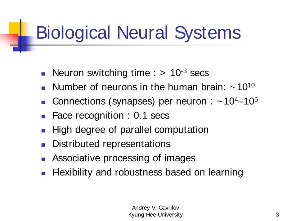
Biological Neural Systems

Neuron switching time : > 10-3 secsNumber of neurons in the human brain: ~1010

Connections (synapses) per neuron : ~104–105

Face recognition : 0.1 secsHigh degree of parallel computationDistributed representationsAssociative processing of imagesFlexibility and robustness based on learning


Properties of Artificial Neural Nets (ANNs)

Many simple neuron-like threshold switching unitsMany weighted interconnections among unitsHighly parallel, distributed processingLearning by tuning the connection weightsSome models provide learning by creation of new neurons


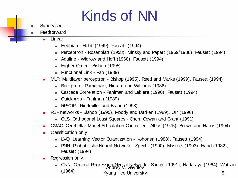
Kinds of NNSupervised Feedforward

Linear Hebbian - Hebb (1949), Fausett (1994) Perceptron - Rosenblatt (1958), Minsky and Papert (1969/1988), Fausett (1994) Adaline - Widrow and Hoff (1960), Fausett (1994) Higher Order - Bishop (1995) Functional Link - Pao (1989)

MLP: Multilayer perceptron - Bishop (1995), Reed and Marks (1999), Fausett (1994) Backprop - Rumelhart, Hinton, and Williams (1986) Cascade Correlation - Fahlman and Lebiere (1990), Fausett (1994) Quickprop - Fahlman (1989) RPROP - Riedmiller and Braun (1993)

RBF networks - Bishop (1995), Moody and Darken (1989), Orr (1996) OLS: Orthogonal Least Squares - Chen, Cowan and Grant (1991)

CMAC: Cerebellar Model Articulation Controller - Albus (1975), Brown and Harris (1994) Classification only

LVQ: Learning Vector Quantization - Kohonen (1988), Fausett (1994) PNN: Probabilistic Neural Network - Specht (1990), Masters (1993), Hand (1982), Fausett (1994)

Regression only GNN: General Regression Neural Network - Specht (1991), Nadaraya (1964), Watson (1964)


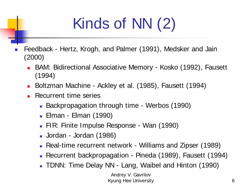
Kinds of NN (2)Feedback - Hertz, Krogh, and Palmer (1991), Medsker and Jain (2000)

BAM: Bidirectional Associative Memory - Kosko (1992), Fausett(1994) Boltzman Machine - Ackley et al. (1985), Fausett (1994) Recurrent time series

Backpropagation through time - Werbos (1990) Elman - Elman (1990) FIR: Finite Impulse Response - Wan (1990) Jordan - Jordan (1986) Real-time recurrent network - Williams and Zipser (1989) Recurrent backpropagation - Pineda (1989), Fausett (1994) TDNN: Time Delay NN - Lang, Waibel and Hinton (1990)


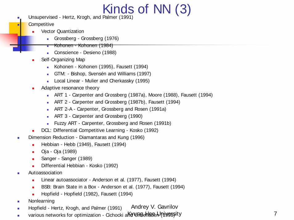
Kinds of NN (3)Unsupervised - Hertz, Krogh, and Palmer (1991) Competitive

Vector Quantization Grossberg - Grossberg (1976) Kohonen - Kohonen (1984) Conscience - Desieno (1988)

Self-Organizing Map Kohonen - Kohonen (1995), Fausett (1994) GTM: - Bishop, Svensén and Williams (1997) Local Linear - Mulier and Cherkassky (1995)

Adaptive resonance theory ART 1 - Carpenter and Grossberg (1987a), Moore (1988), Fausett (1994) ART 2 - Carpenter and Grossberg (1987b), Fausett (1994) ART 2-A - Carpenter, Grossberg and Rosen (1991a) ART 3 - Carpenter and Grossberg (1990) Fuzzy ART - Carpenter, Grossberg and Rosen (1991b)

DCL: Differential Competitive Learning - Kosko (1992) Dimension Reduction - Diamantaras and Kung (1996)

Hebbian - Hebb (1949), Fausett (1994) Oja - Oja (1989) Sanger - Sanger (1989) Differential Hebbian - Kosko (1992)

AutoassociationLinear autoassociator - Anderson et al. (1977), Fausett (1994) BSB: Brain State in a Box - Anderson et al. (1977), Fausett (1994) Hopfield - Hopfield (1982), Fausett (1994)

NonlearningHopfield - Hertz, Krogh, and Palmer (1991) various networks for optimization - Cichocki and Unbehauen (1993)


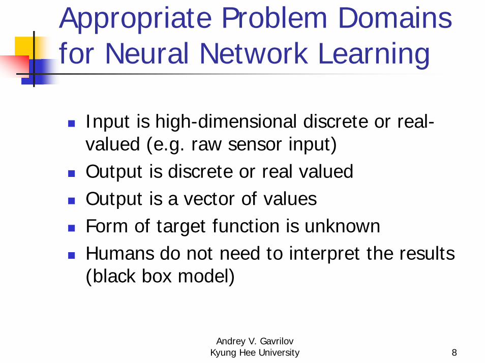
Appropriate Problem Domains for Neural Network Learning

Input is high-dimensional discrete or real-valued (e.g. raw sensor input)Output is discrete or real valuedOutput is a vector of valuesForm of target function is unknownHumans do not need to interpret the results (black box model)


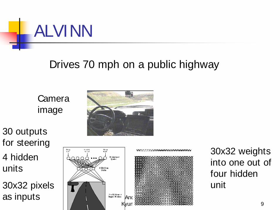
ALVINN

Drives 70 mph on a public highway

Camera image

30x32 pixelsas inputs

30 outputsfor steering

30x32 weightsinto one out offour hiddenunit

4 hiddenunits


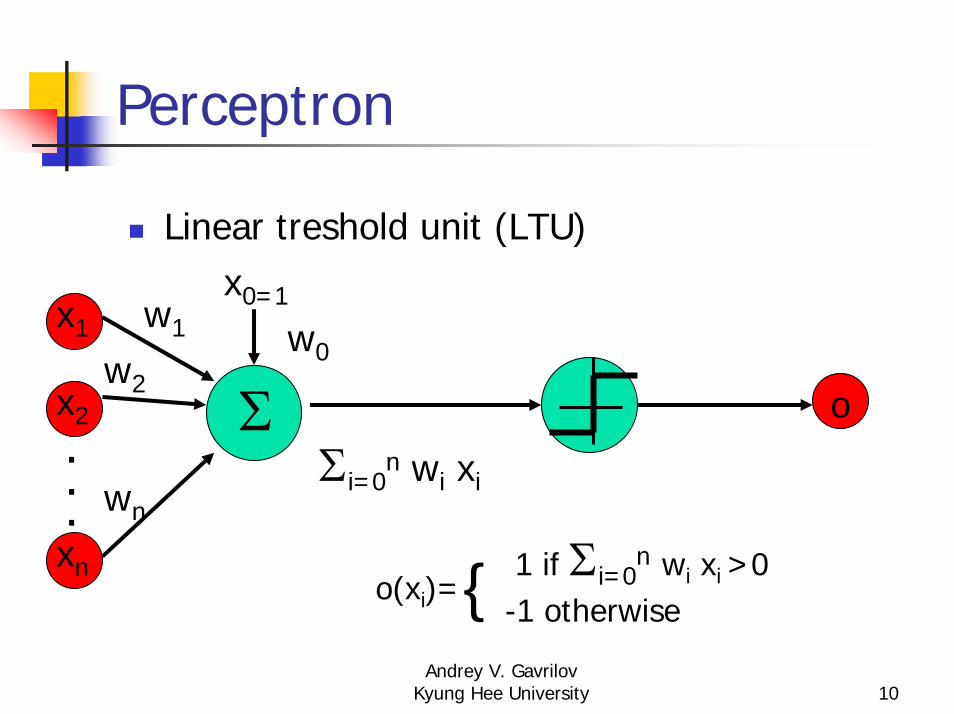
Perceptron

Linear treshold unit (LTU)

Σ

x1

x2

xn

...

w1

w2

wn

x0=1

w0

Σi=0n wi xi

o

1 if Σi=0n wi xi >0

o(xi)= -1 otherwise{


Decision Surface of a Perceptron

x2

+

++

+ -

-

-

-x1

x2

+ -

x1

+-

• Perceptron is able to represent some useful functions• And(x1,x2) choose weights w0=-1.5, w1=1, w2=1• But functions that are not linearly separable (e.g. Xor)

are not representable


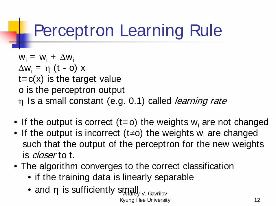
Perceptron Learning Rulewi = wi + ∆wi∆wi = η (t - o) xit=c(x) is the target valueo is the perceptron outputη Is a small constant (e.g. 0.1) called learning rate

• If the output is correct (t=o) the weights wi are not changed• If the output is incorrect (t≠o) the weights wi are changed

such that the output of the perceptron for the new weights is closer to t.

• The algorithm converges to the correct classification• if the training data is linearly separable• and η is sufficiently small


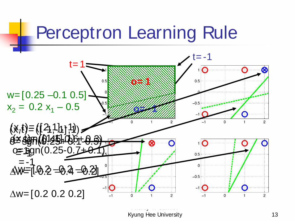
Perceptron Learning Rule

t=1t=-1

w=[0.25 –0.1 0.5]x2 = 0.2 x1 – 0.5

o=1

o=-1

(x,t)=([-1,-1],1)o=sgn(0.25+0.1-0.5)=-1

∆w=[0.2 –0.2 –0.2]

(x,t)=([2,1],-1)o=sgn(0.45-0.6+0.3)=1

∆w=[-0.2 –0.4 –0.2]

(x,t)=([1,1],1)o=sgn(0.25-0.7+0.1)=-1

∆w=[0.2 0.2 0.2]


Gradient Descent Learning Rule

Consider linear unit without threshold and continuous output o (not just –1,1)

o=w0 + w1 x1 + … + wn xn

Train the wi’s such that they minimize thesquared error

E[w1,…,wn] = ½ Σd∈D (td-od)2

where D is the set of training examples


Gradient Descent

D={<(1,1),1>,<(-1,-1),1>,<(1,-1),-1>,<(-1,1),-1>}

Gradient:∇E[w]=[∂E/∂w0,… ∂E/∂wn]

(w1,w2)

(w1+∆w1,w2 +∆w2)∆w=-η ∇E[w]

∆wi=-η ∂E/∂wi

=∂/∂wi 1/2Σd(td-od)2

= ∂/∂wi 1/2Σd(td-Σi wi xi)2

= Σd(td- od)(-xi)


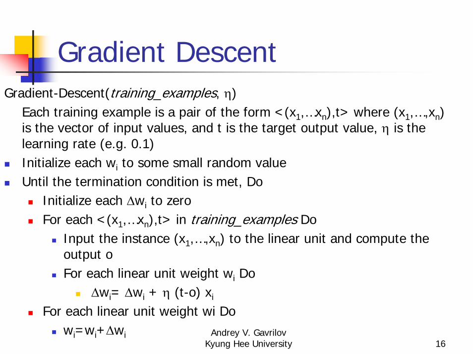
Gradient DescentGradient-Descent(training_examples, η)

Each training example is a pair of the form <(x1,…xn),t> where (x1,…,xn) is the vector of input values, and t is the target output value, η is thelearning rate (e.g. 0.1)Initialize each wi to some small random valueUntil the termination condition is met, Do

Initialize each ∆wi to zeroFor each <(x1,…xn),t> in training_examples Do

Input the instance (x1,…,xn) to the linear unit and compute the output oFor each linear unit weight wi Do

∆wi= ∆wi + η (t-o) xi

For each linear unit weight wi Dowi=wi+∆wi


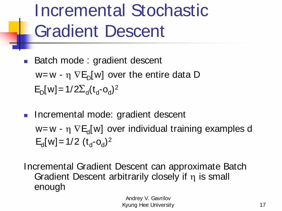
Incremental Stochastic Gradient DescentBatch mode : gradient descentw=w - η ∇ED[w] over the entire data DED[w]=1/2Σd(td-od)2

Incremental mode: gradient descentw=w - η ∇Ed[w] over individual training examples dEd[w]=1/2 (td-od)2

Incremental Gradient Descent can approximate Batch Gradient Descent arbitrarily closely if η is small enough


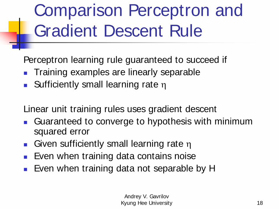
Comparison Perceptron and Gradient Descent Rule

Perceptron learning rule guaranteed to succeed ifTraining examples are linearly separableSufficiently small learning rate η

Linear unit training rules uses gradient descentGuaranteed to converge to hypothesis with minimum squared errorGiven sufficiently small learning rate ηEven when training data contains noiseEven when training data not separable by H


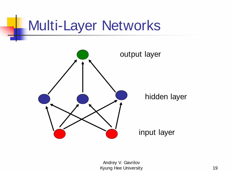
Multi-Layer Networks

output layer

hidden layer

input layer


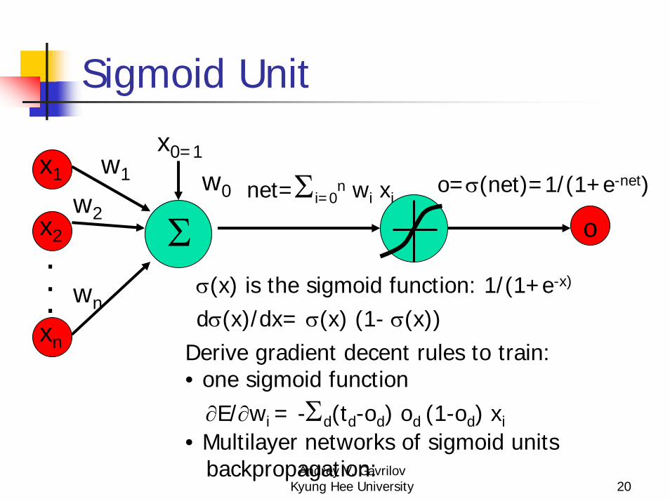
Sigmoid Unit

Σ

x1

x2

xn

...

w1

w2

wn

x0=1

w0 net=Σi=0n wi xi

o

o=σ(net)=1/(1+e-net)

σ(x) is the sigmoid function: 1/(1+e-x)

dσ(x)/dx= σ(x) (1- σ(x))Derive gradient decent rules to train:• one sigmoid function∂E/∂wi = -Σd(td-od) od (1-od) xi

• Multilayer networks of sigmoid unitsbackpropagation:


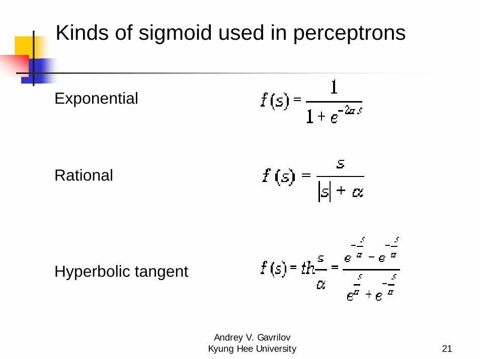
Kinds of sigmoid used in perceptrons

Exponential

Rational

Hyperbolic tangent


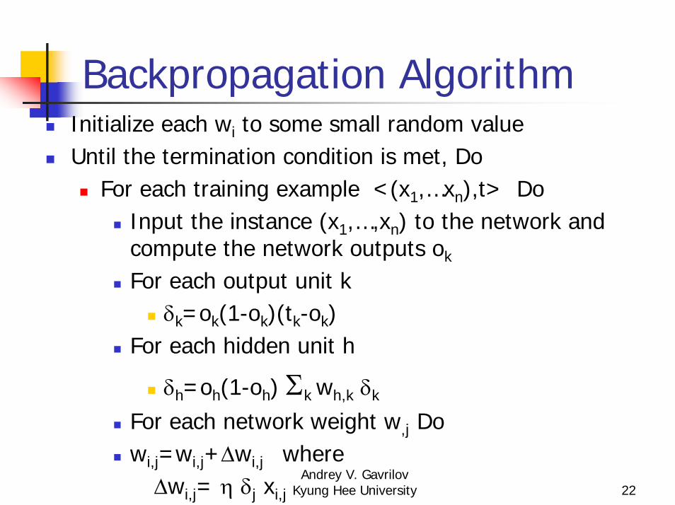
Backpropagation AlgorithmInitialize each wi to some small random valueUntil the termination condition is met, Do

For each training example <(x1,…xn),t> DoInput the instance (x1,…,xn) to the network andcompute the network outputs ok

For each output unit kδk=ok(1-ok)(tk-ok)

For each hidden unit h

δh=oh(1-oh) Σk wh,k δk

For each network weight w,j Dowi,j=wi,j+∆wi,j where∆wi,j= η δj xi,j


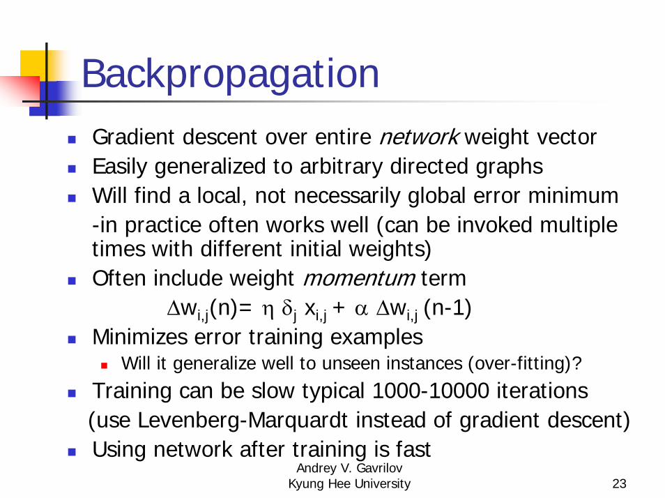
BackpropagationGradient descent over entire network weight vectorEasily generalized to arbitrary directed graphsWill find a local, not necessarily global error minimum-in practice often works well (can be invoked multiple times with different initial weights)Often include weight momentum term

∆wi,j(n)= η δj xi,j + α ∆wi,j (n-1)Minimizes error training examples

Will it generalize well to unseen instances (over-fitting)?Training can be slow typical 1000-10000 iterations(use Levenberg-Marquardt instead of gradient descent)Using network after training is fast


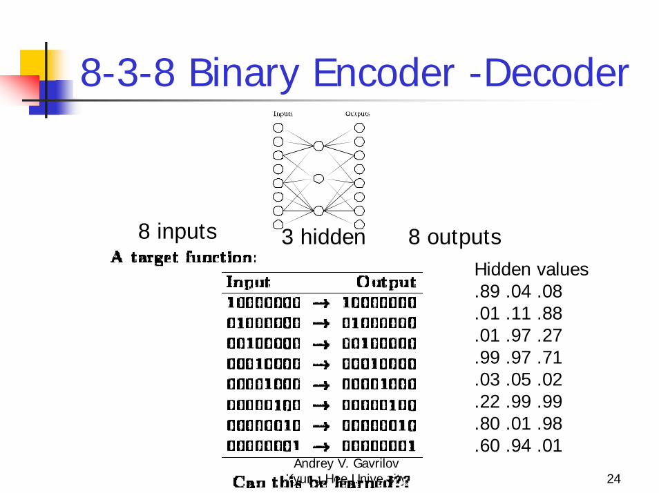
8 inputs 3 hidden 8 outputs

8-3-8 Binary Encoder -Decoder

Hidden values.89 .04 .08.01 .11 .88.01 .97 .27.99 .97 .71.03 .05 .02.22 .99 .99.80 .01 .98.60 .94 .01


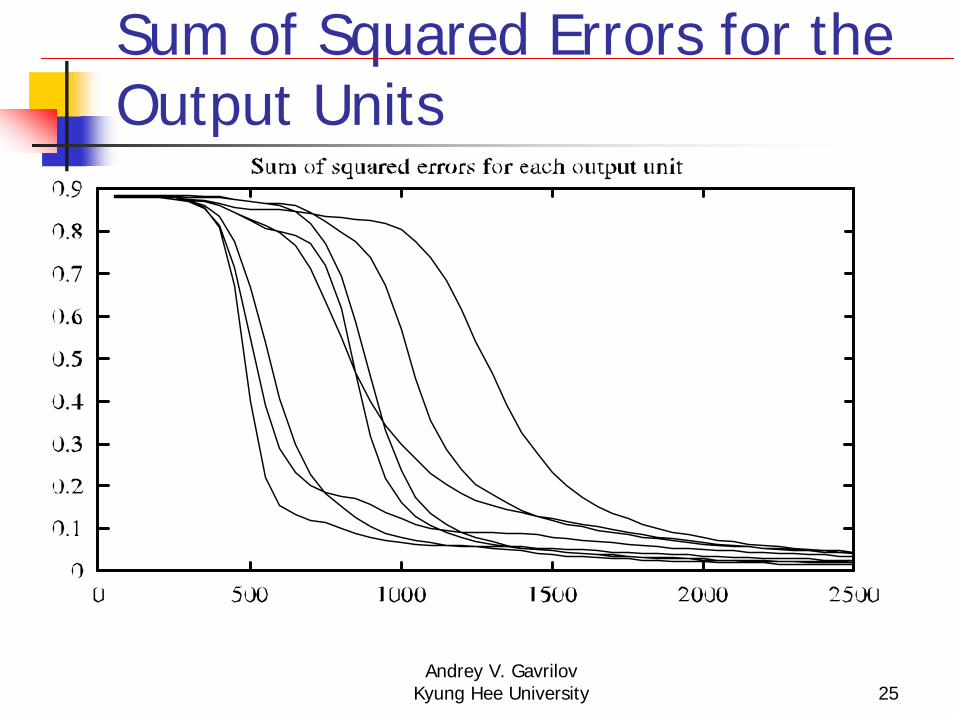
Sum of Squared Errors for the Output Units


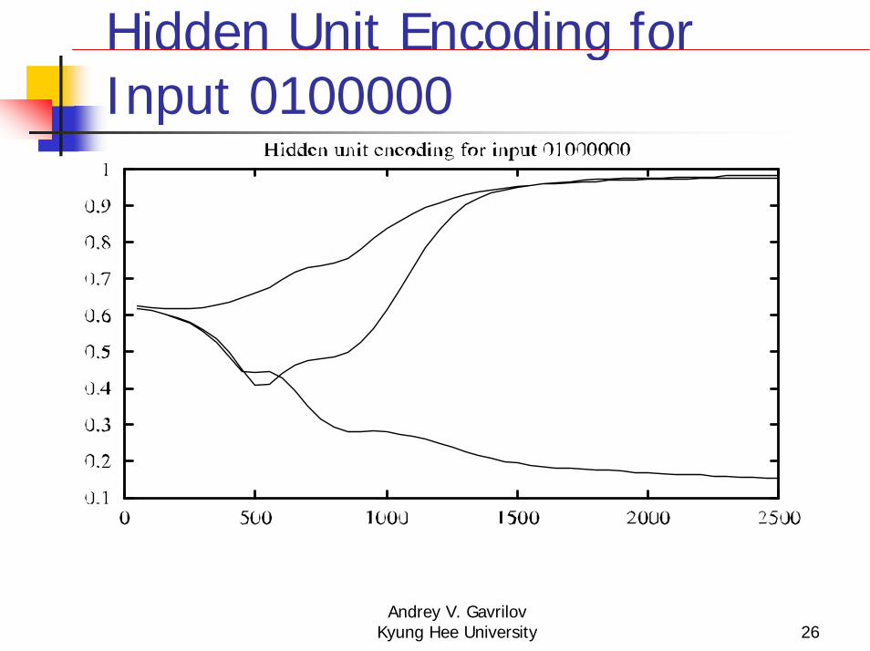
Hidden Unit Encoding for Input 0100000


Convergence of BackpropGradient descent to some local minimum

Perhaps not global minimumAdd momentumStochastic gradient descentTrain multiple nets with different initial weights

Nature of convergenceInitialize weights near zeroTherefore, initial networks are near-linearIncreasingly non-linear functions possible as training progresses


Expressive Capabilities of ANNBoolean functions

Every boolean function can be represented by network with single hidden layerBut might require exponential (in number of inputs) hidden units

Continuous functionsEvery bounded continuous function can be approximated with arbitrarily small error, by network with one hidden layerAny function can be approximated to arbitrary accuracy by a network with two hidden layers


Two tasks solved by MLP

Classification (recognition)Usually binary outputs

Regression (approximation)Analog outputs


Advantages and disadvantages of MLP with back propagation

Advantages:Guarantee of possibility of solving of tasks

Disadvantages:Low speed of learningPossibility of overfittingImpossible to relearningIt is needed to select of structure for solving of concrete task (usually it is problem)


Increase of speed of learning

Preprocessing of features before getting to inputs of perceptonDynamical step of learning (in begin one is large, than one is decreasing)Using of second derivative in formulas for modification of weightsUsing hardware implementation


Fight against of overfitting

Don’t select too small error for learning or too large number of iteration


Choice of structure

Using of constructive learning algorithmsDeleting of nodes (neurons) and links corresponding to one (prunning networks)Appending new neurons if it is needed (growth networks)

Using of genetic algorithms for selection of suboptimal structure


Impossible to relearning

Using of constructive learning algorithmsDeleting of nodes (neurons) and links corresponding to oneAppending new neurons if it is neededThis is incremental learning

lecture 5 artificial neural networks. multi-layer … cerebellar model articulation controller -...

Documents