Lecture 5Coefficient correlation

Coefficient determinationCalibration curve (slope & intercept)

ANALYTICAL CHEMISTRYERT 207

Mid-term preparation

BASIC STATISTICS

Define accuracy and precision, remember ways of describing accuracy and precision, types of errors, understand the concept of significant figures, standard deviation.

UTILIZATION OF STATISTICS IN DATA ANALYSIS

Identify the significant testing. Calculate the T test and Q test.

Wednesday 6 November, 9am

Scatter Plots and Correlation

• A scatter plot (or scatter diagram) is used to show the relationship between two variables

• Correlation analysis is used to measure strength of the association (linear relationship) between two variables

– Only concerned with strength of the relationship

– No causal effect is implied

Scatter Plot Examples

y

x

y

x

y

y

x

x

Linear relationships

Curvilinear relationships

Scatter Plot Examples

y

x

y

x

y

y

x

x

Strong relationships

Weak relationships

Scatter Plot Examples

y

x

y

x

No relationship

Correlation Coefficient

• The population correlation coefficient ρ (rho) measures the strength of the association between the variables

• The sample correlation coefficient r is an estimate of ρ and is used to measure the strength of the linear relationship in the sample observations

Features of ρand r

Unit freeRange between -1 and 1The closer to -1, the stronger the negative

linear relationshipThe closer to 1, the stronger the positive

linear relationshipThe closer to 0, the weaker the linear

relationship

r = +.3 r = +1

Examples of Approximate r Values

y

x

y

x

y

x

y

x

y

x

r = -1 r = -.6 r = 0

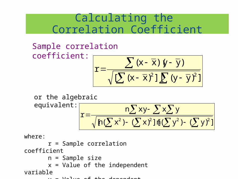
Calculating the Correlation Coefficient

])yy(][)xx([

)yy)(xx(r

22

where:r = Sample correlation coefficientn = Sample sizex = Value of the independent

variabley = Value of the dependent

variable

])y()y(n][)x()x(n[

yxxynr

2222

Sample correlation coefficient:

or the algebraic equivalent:

Example:

You are developing a new analytical method for the determination of blood urea nitrogen (BUN). You want to determine whether your method differs significantly from a standard one for analyzing a range sample concentrations expected to be found in the routine laboratory. It has been ascertained that the two methods have comparable precisions. Following are two sets of the results for a number of individual samples:

Sample Your Method (mg/dL) ,x

Standard Method (mg/dL) ,y

A 10.2 10.5

B 12.7 11.9

C 8.6 8.7

D 7.5 16.9

E 11.2 10.9

F 11.5 11.1

Coefficient of Determination, R2

• The coefficient of determination is the portion of the total variation in the dependent variable that is explained by variation in the independent variable

• The coefficient of determination is also called R-squared and is denoted as R2

SST

SSRR 2 1R0 2 where

Coefficient of Determination, R2

Coefficient of determination

squares of sum total

regressionby explained squares of sum

SST

SSRR 2

Note: In the single independent variable case, the coefficient of determination is

where:R2 = Coefficient of determination

r = Simple correlation coefficient

22 rR

• Total variation is made up of two parts:

SSR SSE SST Total sum of Squares

Sum of Squares Regression

Sum of Squares Error

2)yy(SST 2)yy(SSE 2)yy(SSR

where: = Average value of the dependent variabley = Observed values of the dependent

variable = Estimated value of y for the given x

value

y

y

• SST = total sum of squares

– Measures the variation of the yi values around their mean y

• SSE = error sum of squares

– Variation attributable to factors other than the relationship between x and y

• SSR = regression sum of squares

– Explained variation attributable to the relationship between x and y

Xi

y

x

yi

SST = (yi - y)2

SSE = (yi - yi

)2

SSR = (yi - y)2

_

_

_

Explained and Unexplained Variation

y

y

y_y

R2 = +1

Examples of Approximate R2 Values

y

x

y

x

R2 = 1

R2 = 1

Perfect linear relationship between x and y:

100% of the variation in y is explained by variation in x

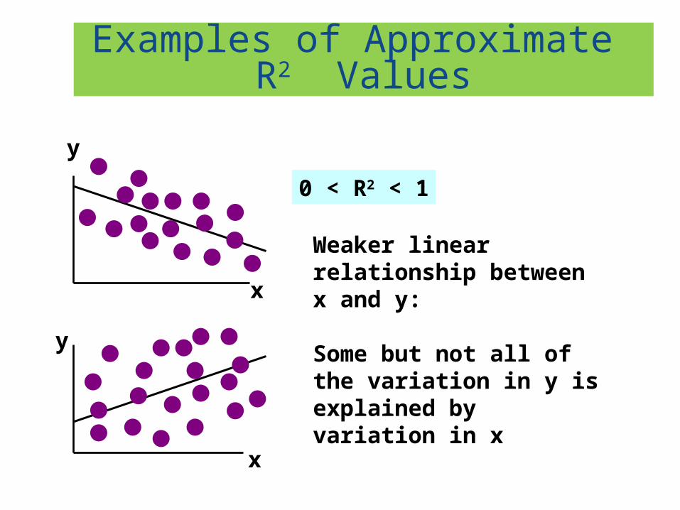
Examples of Approximate R2 Values

y

x

y

x

0 < R2 < 1

Weaker linear relationship between x and y:

Some but not all of the variation in y is explained by variation in x

Examples of Approximate R2 Values

R2 = 0

No linear relationship between x and y:

The value of Y does not depend on x. (None of the variation in y is explained by variation in x)

y

xR2 = 0

Introduction to Regression Analysis

• Regression analysis is used to:– Predict the value of a dependent variable based on

the value of at least one independent variable– Explain the impact of changes in an independent

variable on the dependent variable

Dependent variable: the variable we wish to explain

Independent variable: the variable used to explain the dependent variable

Simple Linear Regression Model

• Only one independent variable, x

• Relationship between x and y is described by a linear function

• Changes in y are assumed to be caused by changes in x

Types of Regression Models

Positive Linear Relationship

Negative Linear Relationship

Relationship NOT Linear

No Relationship

Method of Least Squares

Chemistry 215 Copyright D Sharma

25

Find “best” line by minimizing vertical deviation between the points and the line.

bmxyi

Calculating the Residual

26

Linear RegressionLinear RegressionFitting a straight line to observations

Small residual errors Large residual errorError = (Actual value) – (Predicted value)

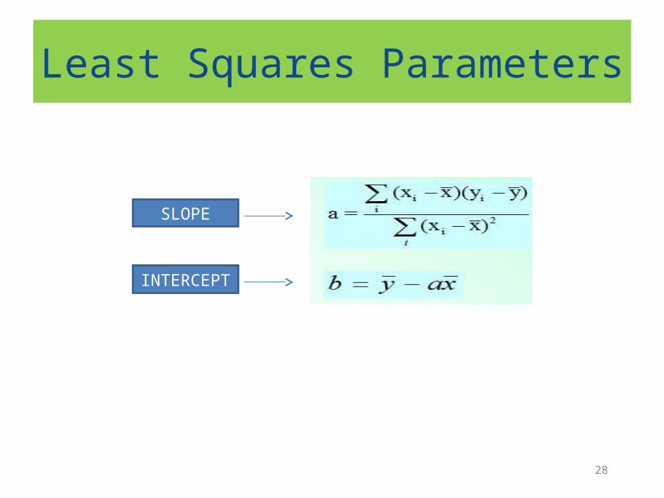
Least Squares Parameters

28

SLOPE

INTERCEPT

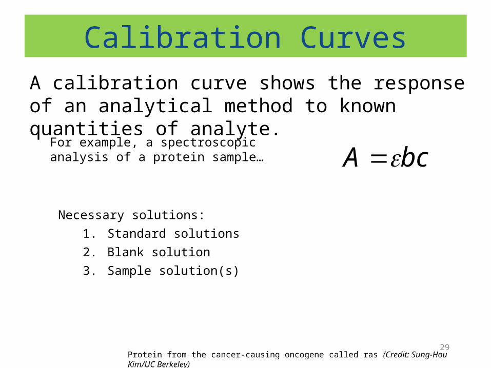
Calibration Curves

29

A calibration curve shows the response of an analytical method to known quantities of analyte.

bcA For example, a spectroscopic analysis of a protein sample…

Necessary solutions:

1. Standard solutions

2. Blank solution

3. Sample solution(s)

Protein from the cancer-causing oncogene called ras (Credit: Sung-Hou Kim/UC Berkeley)

Constructing a Calibration Curve

30

Spectroscopic analysis of a protein sample…

Constructing a Calibration Curve

31

Equation of linear response

y = m (x) + b

Abs = m (µg protein) + b

y = 0.0163 (x) +0.004

…where y is the corrected abs.

Determine the unknown concentration based on its absorbance

Determination of an unknown value (x) based on its response (y)Spectroscopic analysis of a protein sample…cont.

Tips for Calibrating InstrumentsKnow the limitations of your instrument

◦ Limits of detection (or LOD) ◦ Range of linearity

Watch-out for interferences◦ Overlapping spectral responses (e.g., from impurities) ◦ Unwanted sample precipitation

Use serial dilutions where possible◦ Less error than preparing individual samples

32

Serial Dilution (A Review)

33

34

Using spreadsheet for plotting calibration curves

Some useful statistical syntaxes:1.AVERAGE = mean of series of number2.MEDIAN = median of series of number3.STDEV = standard deviation4.VAR = variance5.RSQ = R- squared

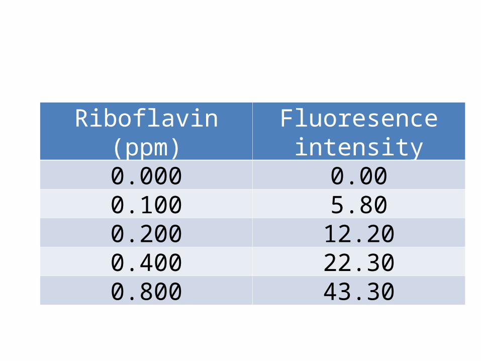
Riboflavin (ppm) Fluoresence intensity0.000 0.000.100 5.800.200 12.200.400 22.300.800 43.30

Slope, intercept and coefficient determination

We can use the Excel statistical functions to calculate the slope and intercept for a series of data , and the R2 value without a plot

Open a new spreadsheet and enter the calibration data from the previous example.

In cell A9 type INTERCEPT, cell A10, SLOPE AND cell A11, R-Squared.

Highlight cell B9Click on fx: StatisticalAnd scroll down to INTERCEPT and click OK

• For known_x’s, enter the array A3:A7 and for known_y’s, enter B3:B7, then click OK.

• The INTERCEPT is displayed in cell B9.• Now repeat , highlighting cell B10, scrolling to

SLOPE , and entering the same arrays. The Slope appears in cell B10.

• Followed the same way for R-squared.

Exercise

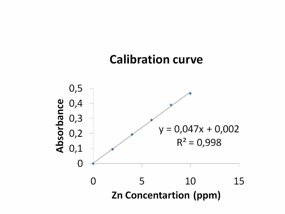
• The following data were obtained to get a calibration curve for the determination of Zn in the wastewater by using atomic absorption spectrometry (AAS). Using calculator or computer, plot the data and find the best straight line equation and correlation determination.

Zn concentration (ppm) Absorbance

0 0

2 0.095

4 0.194

6 0.290

8 0.390

10 0.466

• Solution:• The equation of the straight line is:Y =0.047X + 0.002Correlation determination (R2) = 0.998